Abstract

We study the abilities of the Fermi–LAT instrument on board of the Fermi mission to simultaneously constrain the Milky Way dark matter density profile and some dark matter particle properties, as annihilation cross section, mass and branching ratio into dominant annihilation channels. A single dark matter density profile is commonly assumed to determine the capabilities of gamma-ray experiments to extract dark matter properties or to set limits on them. However, our knowledge of the Milky Way halo is far from perfect, and thus in general, the obtained results are too optimistic. Here, we study the effect these astrophysical uncertainties would have on the determination of dark matter particle properties and conversely, we show how gamma-ray searches could also be used to learn about the structure of the Milky Way halo, as a complementary tool to other type of observational data that study the gravitational effect caused by the presence of dark matter. In addition, we also show how these results would improve if external information on the annihilation cross section and on the local dark matter density were included and compare our results with the predictions from numerical simulations.

1 Introduction

One of the mysteries of modern physics is the presence of an unknown non-luminous and non-baryonic matter in the Universe (see Refs. [1, 2, 3, 4, 5] for reviews), the so-called dark matter (DM). However, although there are many pieces of evidence in favor of the existence of DM and which indicate that it constitutes about 80% of the total mass of the Universe [6, 7, 8], it is worth noting that they each infer DM’s presence uniquely through its gravitational influence. In other words, we currently have no conclusive evidence for DM’s non-gravitational interactions. Thus, the origin and most of the properties of DM (mass, spin, couplings) remain unknown.

Although many particles have been proposed as DM candidates (see, e.g., Refs. [4, 9] for a comprehensive list), a weakly interacting massive particle (WIMP), with mass lying from the GeV to the TeV scale, is one of the most popular ones. WIMPs can arise in extensions of the Standard Model such as supersymmetry (e.g., Ref. [1]), little Higgs (e.g., Ref. [10]) or extra-dimensions models (e.g., Ref. [11] ) and are usually stable and thermally produced in the early Universe with an annihilation cross section (times relative velocity) of $\langle\sigma v\rangle\sim 3\times 10^{-26}$ cm³/s, which is the standard value that provides the observed DM relic density. Thus, WIMPs are cold DM (CDM) candidates.

Within the framework of CDM, as favored by observations, structure forms hierarchically bottom-up, with DM collapsing first into small halos, which then accrete matter, merge and eventually give rise to larger halos [12, 13, 14]. Within this paradigm, the properties of luminous galaxies are expected to be related to those of DM halos [15], which carry with them gas that cools and collapses to their center to form galaxies.

Over the past decades, the progress in high-resolution N-body simulations has permitted a better understanding of the structure of CDM halos. It has been shown that density profiles of CDM halos can be reasonably well described by an universal form, independent of the halo mass, which predicts cuspy mass distributions. Although the first analytical analysis of this kind predicted that the radial distribution of DM follows a simple power-law [16], it was later shown with N-body simulations that the slope of the DM distribution is not constant and changes with the distance to the center of the halo. It was Navarro, Frenk and White (NFW) who first proposed a simple two-parameter fitting formula to describe spherically averaged DM density profiles [17, 18]. However, further simulations with improved numerical resolution started to show some systematic differences [19, 20, 21, 22, 23, 24, 25, 26, 27, 28, 29, 30, 31, 32], mainly in the innermost regions of CDM halos. Thus, in order to reproduce several of these features, as the gradual shallowing of the density profile towards the center of the halo, an improved three-parameter fitting formula was proposed [33], the so-called Einasto profile [34].

Nevertheless, these prescriptions only represent the mean of all simulated halos for a given mass at a given redshift. The scatter with respect to these mean values [35, 36, 37, 38, 39, 40] is thought to be related to the different halo formation histories and to the evolution of the expanding Universe [18, 41, 42, 43, 44, 45, 46, 47, 48, 49]. Thus, these average values do not necessarily describe accurately the DM halo of our own Galaxy. Indeed, it is not clear that the Milky Way is a prototypical spiral galaxy. For instance, while the presence of the two Magellanic Clouds points to a more massive halo, this would also imply higher chances for a recent merger that could have destroyed the thin galactic disc [50].

However, probing the inner structure of the Milky Way DM halo is a very challenging task and current data do not allow to distinguish among different density profiles [51, 52]. This is particularly important for the astrophysical detection of DM, as these searches are critically sensitive to the structure of the Milky Way DM halo. Direct detection experiments, searching for signals of nuclear recoil of DM scattering off nuclei, depend on the local DM density and velocity distribution. On the other hand, indirect searches look for the products of DM annihilation (or decay), which include antimatter, neutrinos and photons. In the case of DM annihilation, the luminosity depends quadratically on the DM density and the largest uncertainties come from the region where we expect the highest (neutrino or gamma-ray) signal, i.e., the galactic center (GC). Hence, a better understanding of the Milky Way halo is required to determine the potential reach of current and future experiments. Conversely, astrophysical searches, and in particular indirect DM gamma-ray searches, could also be used to learn about the distribution of DM in the innermost regions of the Milky Way halo, beyond the limit of convergence of numerical simulations. Thus, in case of a positive signal, these searches could be useful not only to learn about the DM nature, but also as a complementary tool to constrain the Milky Way DM density profile, which may not be necessarily representative of the general characteristics obtained in numerical simulations.

In this work, we study the abilities of the Large Area Telescope (Fermi–LAT) instrument on board of the Fermi Gamma-ray Space Telescope (Fermi) mission [53] to constrain the DM density profile and the effect the uncertainties in the DM distribution could have to constrain DM properties, as annihilation cross section, mass and branching ratio into dominant annihilation channels. We consider the potential gamma-ray signal in a squared region with a side of $20^{\circ}$ around the GC ($|l|,|b|<10^{\circ}$) and, in order to model the relevant gamma-ray foregrounds, we use the numerical code GALPROP [54] and the latest Fermi–LAT observations [55, 56].

During the last years, different approaches have been proposed to determine the WIMP DM properties by using indirect or direct measurements or their combination [57, 58, 59, 60, 61, 62, 63, 64, 65, 66, 67, 68, 69, 70, 71, 72, 73, 74, 75, 76, 77, 78, 79, 80, 81, 82, 83, 84, 85, 86, 87, 88, 89]. In addition, the information that could be obtained from collider experiments would also be of fundamental importance to learn about the nature of DM [90, 91, 92, 93, 94, 95, 96, 97, 98, 99, 100, 101, 102, 103, 104, 105] and could also be further constrained when combined with direct and indirect detection data [58, 98, 106, 107, 108]. Therefore, in order to show how well the DM density profile could be determined by the combination of different type of experiments, we will also make use of potential information that might be obtained on some parameters by other complementary means in addition to the gamma-ray signal.

The paper is organized as follows. In Section 2 we describe the most relevant (for this work) component of the gamma-ray emission from DM annihilation in the GC. In Section 3 we state some of the results obtained in numerical N-body simulations regarding the density profiles of CDM halos and we also briefly review the current knowledge of some of the most important parameters that determine the structure of the Milky Way halo. We describe the ingredients of our analysis in Section 4 and present the results in Section 5. Finally, we draw our conclusions in Section 6.

2 Gamma-rays from DM annihilations

The differential flux of prompt gamma–rays generated from DM annihilations in the smooth Milky Way DM halo  after the hadronization, fragmentation and decay of the final states and coming from a direction within a solid angle $\Delta\Omega$ can be written as [112]

$$\left(\frac{d\Phi_{\gamma}}{dE_{\gamma}}\right)_{{\rm prompt}}(E_{\gamma},\Delta\Omega)=R_{\odot}\,\rho_{\odot}^{2}\,\overline{J}(\Omega)\,\frac{\Delta\Omega}{4\,\pi}\,\frac{\langle\sigma v\rangle}{2\,m_{\chi}^{2}}\,\sum_{i}\text{BR}_{i}\,\frac{dN_{\gamma}^{i}}{dE_{\gamma}}\leavevmode\nobreak\ ,$$ (1)

where $R_{\odot}$ is the distance from the Sun to the GC, $\rho_{\odot}=\rho(R_{\odot})$ is the local DM density, $\langle\sigma v\rangle$ is the thermal average of the total annihilation cross section times the relative velocity, $m_{\chi}$ is the DM mass, the discrete sum is over all DM annihilation channels, BR_i is the branching ratio of DM annihilation into the $i$-th final state and $dN_{\gamma}^{i}/dE_{\gamma}$ is the differential gamma–ray yield of SM particles into photons for the $i$-th channel, that we simulate with the event generator PYTHIA 6.4 [113], which automatically includes the so-called final state radiation (photons radiated off the external legs). The dimensionless quantity $\overline{J}$, which depends crucially on the DM distribution, is defined as

$$\overline{J}(\Omega)=\frac{1}{\Delta\Omega}\,\frac{1}{R_{\odot}\,\rho_{\odot}^{2}}\,\int_{\Delta\Omega}d\Omega\,\int_{\text{los}}\rho\big{(}r(s,\Omega)\big{)}^{2}\ ds\,\leavevmode\nobreak\ ,$$ (2)

where the spatial integration of the square of the DM density profile $\rho(r)$ is performed along the line of sight within the solid angle of observation $\Delta\Omega$. More precisely, the distance from the GC is $r=\sqrt{R^{2}_{\odot}-2\,s\,R_{\odot}\cos\psi+s^{2}}$, and the upper limit of integration is $s_{\rm max}=\sqrt{(R_{\rm vir}^{2}-\sin^{2}\psi\,R^{2}_{\odot})}+R_{\odot}\cos\psi$, where $\psi$ is the angle between the direction of the GC and that of observation. The virial radius of the Milky Way DM halo is defined as $R_{\rm vir}=\left[3\,M_{\rm vir}/(4\pi\,\Delta_{\rm vir}\,\rho_{\rm crit})\right]^{1/3}$, where $M_{\rm vir}$ is the virial mass of the DM halo, $\rho_{\rm crit}$ is the critical density of the Universe and $\Delta_{\rm vir}=18\pi^{2}+82\,(\Omega_{\rm m}-1)-39\,(\Omega_{\rm m}-1)^{2}$ is the virial overdensity [114] with $\Omega_{\rm m}=0.258$ [7] the non-relativistic matter contribution to the total density of the Universe. It is also customary to define the concentration parameter as $c_{\rm vir}\equiv R_{\rm vir}/r_{s}$, where $r_{s}$ is the scale radius.

3 Milky Way DM density profile

During the past two decades, the improvement in numerical simulations has led to the discovery of a universal internal structure for spherically averaged DM halos [17, 18] that can be well described by a density profile (NFW parametrization) with two (free) parameters given by

$$\rho(r)=\rho_{\odot}\,\frac{\left(R_{\odot}/r_{s}\right)\left[1+(R_{\odot}/r_{s})\right]^{2}}{(r/r_{s})\,[1+(r/r_{s})]^{2}}\leavevmode\nobreak\ .$$ (3)

However, further simulations with improved numerical resolution started to show some systematic differences, mainly in the central regions of CDM halos, that have created a vivid debate [19, 20, 21, 22, 23, 24, 25, 26, 27, 28, 29, 30, 31, 32]. The recent Via Lactea II simulations [110] seem to partly verify earlier results, with a NFW density profile. On the other hand, the Aquarius project simulations [111] seem to favor a slightly different parametrization [33, 115, 116, 117, 118], which is less cuspy towards the center of the Galaxy than the NFW profile and has three (free) parameters, the so-called Einasto profile [34],

$$\rho(r)=\rho_{\odot}\,\exp\left[-\frac{2}{\alpha}\left(\left(\frac{r}{r_{s}}\right)^{\alpha}-\left(\frac{R_{\odot}}{r_{s}}\right)^{\alpha}\right)\right]\leavevmode\nobreak\ ,$$ (4)

which is the same relation between slope and radius that defines Sérsic’s model [119], but applied to space density instead of the projected surface density of galaxies [120].

In order to observationally determine the parameters of the DM density distribution, different constraints are considered. For instance, several dynamical tracers have been used to determine the Milky Way mass , and most estimates have come from escape velocity arguments or from Jeans modeling of the radial density and velocity dispersion profiles of distant halo tracer populations, as satellite galaxies, globular clusters and horizontal branch halo stars on far orbits. However, while the mass of external galaxies can be determined with reasonable precision, the mass of the Milky Way remains uncertain within a factor of $\sim$ 6 ($5\times 10^{11}\,{\rm M}_{\odot}\lesssim M_{\rm MW}\lesssim 3\times 10^{12}\,{\rm M}_{\odot}$) [121, 122, 123, 124, 125, 126, 127, 128, 51, 52, 129, 130, 131, 132] due to the lack of observational data for luminous tracers in its outer regions where DM dominates. Within the innermost $\sim 50-60$ kpc of the Milky Way, on the high mass end we find $M_{\rm MW}(<50\leavevmode\nobreak\ {\rm kpc})\equiv M_{\rm MW}(50)=\left(5.4^{+0.2}_{-3.6}\right)\times 10^{11}\,{\rm M}_{\odot}$ [122], whereas a lower mass was recently obtained by estimating the circular velocity curve up to 60 kpc, $M_{\rm dh}(<60\leavevmode\nobreak\ {\rm kpc})\equiv M_{\rm dh}(60)=(4.0\pm 0.7)\times 10^{11}\,{\rm M}_{\odot}$ [128]. Here $M_{\rm MW}(r)$ and $M_{\rm dh}(r)$ refer to the total mass (dark and visible) of the Milky Way and the DM halo mass within a radius $r$, respectively. Below we will compare these estimates with the masses for the profiles we consider, but we stress that the former estimate refers to the total mass within a given radius and not only to the mass of the DM halo. The galactic disc and bulge (visible matter) are estimated to contribute with a total mass about an order of magnitude lower, $\sim(5-7)\times 10^{10}M_{\odot}$ [133, 134, 132], which would bring the former estimate closer to the latter one.

The local DM density ($\rho_{\odot}$) is another important parameter in the description of the DM halo. This is, as well, a crucial parameter in direct DM detection experiments and in the search for neutrinos produced by DM annihilations at the center of the Sun or the Earth. Commonly, the way to estimate the local DM density follows the approach of Ref. [135] and it is based in constructing three-component (disc, bulge and dark halo) models for the galaxy and confront them against observational data. It is usually assumed to be $\rho_{\odot}=0.3$ GeV/cm³, although approximately with a factor of two of uncertainty. However, this estimate is just a rough central value within the range obtained by several analyses from old dynamical constraints and using cored DM profiles [136]. Moreover, it is curious to note that in these early estimates, to the best of our knowledge, there is no justification for using that particular value, which is not even an unweighted average, but on the contrary, $\rho_{\odot}$ was usually quoted to be slightly larger, e.g., $\rho_{\odot}=0.51^{+0.21}_{-0.17}$ GeV/cm³ [136].

Recently, a few new analyses have been performed using new data. Some of them follow the approach of Ref. [135] but with a large set of new observational constraints of the Milky Way [51, 52, 79, 137, 132] and in Ref. [138] a new technique is proposed such that only local observables are used and there is no need of a model for the galaxy. In general, they tend to obtain slightly larger values than the canonical one, $\rho_{\odot}=0.39\pm 0.03$ GeV/cm³ [51], $\rho_{\odot}=0.32\pm 0.07$ GeV/cm³ [79], $\rho_{\odot}=0.43\pm 0.15$ GeV/cm³ [138], $\rho_{\odot}=0.40\pm 0.04$ GeV/cm³ [132]. Let us also note that DM halos are not predicted to be perfectly spherical and this possible flattening could imply a larger DM local density [136, 139]. In this work we will take $\rho_{\odot}=0.4$ GeV/cm³ as our default value.

Correlated with the use of the DM local density is the knowledge of the distance to the GC ($R_{\odot}$), which is also an important parameter to determine the structure of the Milky Way. It is usually assumed that $R_{\odot}=8.5$ kpc. However, this is based on an old recommendation by the International Astronomical Union, after the value for the unweighted average of $R_{\odot}$ obtained using different estimates between 1974 and 1986 [140]. Nevertheless, after a more careful statistical analysis of these results, which tried to account for statistical and systematic errors and the covariance among the different methods, a lower value of $R_{\odot}=8.0\pm 0.5$ kpc was proposed almost twenty years ago [141]. Many new measurements were performed during the following decade, with an average value $R_{\odot}=7.80\pm 0.33$ kpc [142], consistent within errors with previous estimates.

During the last years, and using new astrometric and radial velocity measurements of stellar orbits around the massive black hole in the GC, new analyses seem to point to a slightly larger value, $R_{\odot}=8.4\pm 0.4$ kpc [143], $R_{\odot}=8.33\pm 0.35$ kpc [144], $R_{\odot}=8.2\pm 0.5$ kpc [145]. In addition, based on trigonometric parallax observations of star forming regions, a similar result has been derived, $R_{\odot}=8.4\pm 0.6$ kpc [146] (see however Ref. [147]). All in all, even with these seemingly converging results, recent measurements still span in the range between $R_{\odot}=7.2\pm 0.3$ kpc [148] and $R_{\odot}=8.7^{+0.57}_{-0.43}$ kpc [149]. In this work, we will take $R_{\odot}=8.3$ kpc as our default value.

From Eqs. (3) and (4), we see that the DM density profile is determined by two parameters in the NFW case ($\rho_{\odot},\,r_{s}$) and three for the Einasto profile ($\rho_{\odot},\,r_{s},\,\alpha$). Nevertheless, one could equivalently use any set of (free) parameters to describe the DM density profile with a given parametrization. For instance, in N-body simulations, it is usually convenient to use the virial mass and the concentration parameter instead of the local DM density and the scale radius. On the other hand, it turns out that different analyses, which make use of the results from N-body simulations, have shown that the structural properties of DM halos depend on the halo mass [18, 35, 36, 37, 39, 40, 41, 42, 43, 44, 45, 46, 47, 48, 49]. In general, the correlations among different parameters also embed the dependence on the cosmological parameters. In particular, these analyses have found an anti-correlation between $M_{\rm vir}$ and $c_{\rm vir}$, which is especially sensitive to the value of $\sigma_{8}$ (a measurement of the amplitude of the linear power spectrum on the scale of 8 $h^{-1}$ Mpc). The median relation between $M_{\rm vir}$ and $c_{\rm vir}$ (assuming a NFW profile) at redshift $z=0$ and for relaxed halos , using the cosmological parameters from the 5-year release of the WMAP mission [7], is given by [49]

$$c_{\rm vir}=10^{2.155}\,\left(\frac{M_{\rm vir}}{h^{-1}{\rm M}_{\odot}}\right)^{-0.097}=10.11\,\left(\frac{M_{\rm vir}}{10^{12}\,{\rm M}_{\odot}}\right)^{-0.097}\leavevmode\nobreak\ ,$$ (5)

where $h=0.72$ [7]. Hence, this type of correlation would reduce further the number of parameters to describe the DM density profile to one (to two in the analogous case of the Einasto profile). However, it is important to bare in mind that Eq. (5) represents the mean concentration for a given virial mass, so it does not account for the intrinsic scatter about these mean relation [35, 36, 37, 39, 40]. The distribution of the logarithm is approximately Gaussian and at $1\sigma$ is typically $\sigma_{\ln c_{\rm vir}}\simeq 0.3$ [35, 36, 37, 38, 39, 40] (see however Ref. [151] where instead of a log-normal distribution of halo concentrations, a Gaussian distribution is found and where also the uncertainty in DM annihilation from the Milky Way halo that arises from the distribution of halo concentrations is discussed). In the analysis that follows, we will also consider the possibility that the Milky Way satisfies this mean relation (Eq. (5)) obtained in numerical N-body simulations.

4 Analysis

The Fermi telescope [53] was launched in June $2008$ for a mission of 5 to 10 years. Fermi–LAT is the primary instrument on board of the Fermi mission and it performs an all-sky survey with a field of view $\text{FoV}=2.4$ sr, covering an energy range from below 20 MeV to more than $300$ GeV for gamma-rays, with an energy and angle-dependent effective area which is approximately $A_{\text{eff}}\simeq 8000$ cm². We consider a constant effective area, but we notice that different effects could reduce the exposure after a more detailed description of the detector is considered, which however is beyond the scope of this paper. Fermi–LAT’s equivalent Gaussian $1\sigma$ energy resolution is $\sim 10\%$ at energies above 1 GeV. On the other hand, for normal incidence, 68% of the photons at 10 GeV are contained within $\sim 0.25^{\circ}$. In the following analysis, we consider a 5-year mission run, an energy interval from 1 GeV to 300 GeV and a square region of observation with a side of $20^{\circ}$ around the GC ($|l|,|b|<10^{\circ}$). In our simplified modeling of the detector, we do not explicitly compute the effects of the energy resolution and of the point spread function. However, in order to avoid that this affects significantly our results, we divide the energy interval into 20 evenly spaced logarithmic bins and consider 10 concentric $1^{\circ}$ bins. Our aim is to illustrate the issues here discussed and serve as a starting analysis for more detailed ones.

In order to study the capabilities of the Fermi–LAT experiment to simultaneously constrain some DM particle properties and the Milky Way DM density profile, we begin by modeling the background. We consider the three components contributing to the high-energy gamma-ray background: the diffuse galactic emission (DGE), the contribution from resolved point sources (PS) and the isotropic gamma-ray background (IGRB). We model the DGE with the GALPROP code (v54) [54] by means of the WebRun service [152] and we take the conventional model, which reproduces reasonably well the recent measurements by Fermi–LAT, at least at intermediate galactic latitudes $10^{\circ}<|b|<20^{\circ}$ and up to 10 GeV [153, 154]. The other two sources of background are taken from the Fermi–LAT published results [55, 56]. We refer the reader to Ref. [61] for further details on the gamma–ray foregrounds we consider. However, let us note that Ref. [61] makes use of the Fermi Science Tools, both to model the background and the signal. We have checked that our simplified modeling of the detector and backgrounds does not introduce significant changes in our results and allow us to substantially reduce the time of computation without modifying our conclusions.

During the last years, different approaches have been considered to constrain WIMP DM properties by using indirect searches, direct detection measurements, collider information or their combination [57, 58, 59, 60, 61, 62, 63, 64, 65, 66, 67, 68, 69, 70, 71, 72, 73, 74, 75, 76, 77, 78, 79, 80, 81, 82, 83, 84, 85, 86, 87, 88, 89, 90, 91, 92, 93, 94, 95, 96, 97, 98, 99, 100, 101, 102, 103, 104, 105, 106, 107, 108]. These measurements are complementary and constitute an important step toward identifying the particle nature of DM. However, astrophysical searches are hindered by large uncertainties in the structure of the Milky Way DM halo and, although different profiles have been considered, it is customary to assume a given DM density profile in order to study the capabilities of gamma-ray experiments to extract some DM properties [57, 58, 59, 60, 61, 62] (for attempts to also fit the DM density profile see Ref. [57], but assuming the annihilation channel to be known and Refs [155, 156], but for a very large annihilation cross section).

In this work, we discuss the Fermi–LAT’s abilities to constrain the DM density profile and some DM properties after 5 years of data taking. We evaluate the effect the uncertainties in the DM density profile could have on the determination of the DM mass, annihilation cross section and the annihilation channels. Concerning the DM density profile, when we consider an Einasto profile, we fit its three parameters: the DM local density $\rho_{\odot}$, the scale radius $r_{s}$ and the index $\alpha$; whereas for the case of a NFW profile we fit $c_{\rm vir}$ and $M_{\rm vir}$. In principle, as with respect to DM properties, the analysis should include all possible annihilation channels, but this would render the present analysis very much time consuming. Nevertheless, in practice, they are commonly classified as hadronic (soft channels) and leptonic channels (hard channels). Thus, for simplicity, when simulating a signal, we only consider two possible (generic) channels, $\tau^{+}\tau^{-}$ or $b\bar{b}$ . By using this simplification, we can reduce the number of total free parameters to six for the Einasto profile and five for the NFW profile: the mass, $m_{\chi}$, the annihilation cross section, $\langle\sigma v\rangle$, the branching ratio into channel 1, $\text{BR}_{1(2)}$ (or equivalently into channel 2, $\text{BR}_{2(1)}=1-\text{BR}_{1(2)}$) and the parameters describing the DM density profile $(\rho_{\odot},r_{s},\alpha)$ or $(M_{\rm vir},c_{\rm vir})$ for the Einasto or NFW profile, respectively. In order to focus on the determination of these parameters and to avoid adding more parameters to the analysis, we assume perfect knowledge of the background. Hence, in this regard, the results here presented should be taken as the most optimistic ones. We use the $\chi^{2}$ function defined as

$$\chi^{2}\left({\bf\theta}\right)=\sum_{j=1}^{10}\sum_{i=1}^{20}\frac{\left(S_{ij}\left({\bf\theta}\right)-S_{ij}^{\text{th}}\left({\bf\theta^{0}}\right)\right)^{2}}{(\sigma_{\rm stat})_{ij}^{2}+(\sigma_{\rm sys})_{ij}^{2}}\leavevmode\nobreak\ ,$$ (6)

where $S_{ij}({\bf\theta})$ represents the simulated signal events in the $i$-th energy and $j$-th angular bin for each set of the parameters ${\bf\theta}=\left(\rho_{\odot},\,r_{s},\,\alpha,\,m_{\chi},\,\langle\sigma v\rangle,\,\text{BR}_{\tau(b)}\right)$ for the case of the Einasto profile or ${\bf\theta}=\left(M_{\rm vir},c_{\rm vir},\,m_{\chi},\,\langle\sigma v\rangle,\,\text{BR}_{\tau(b)}\right)$ for the NFW profile, and $S_{ij}^{\text{th}}({\bf\theta^{0}})$ is the assumed observed signal events in that bin with parameters ${\bf\theta^{0}}=\left(\rho_{\odot}^{0},\,r_{s}^{0},\,\alpha^{0},\,m_{\chi}^{0},\,\langle\sigma v\rangle^{0},\,\text{BR}_{\tau(b)}^{0}\right)$ for the Einasto profile or ${\bf\theta^{0}}=\left(M_{\rm vir}^{0},\,c_{\rm vir}^{0},\,m_{\chi}^{0},\,\langle\sigma v\rangle^{0},\,\text{BR}_{\tau(b)}^{0}\right)$ for the NFW profile. The statistical errors are given by

$$(\sigma_{\rm stat})_{ij}^{2}=S_{ij}^{\text{th}}\left({\bf\theta^{0}}\right)+B_{ij}\leavevmode\nobreak\ ,$$ (7)

where $B_{ij}$ is the number of background events in the $i$-th energy and $j$-th angular bin. On the other hand, in the analysis of Ref. [56], the rms of the residual count fraction between Fermi–LAT data and the DGE model for energies above 200 MeV is larger than the expected statistical errors by a factor of $\sim$ 2.5. Hence, baring in mind that the number of events in each bin is in general dominated by the background events, we conservatively take the systematic errors to be three times the statistical ones, i.e., $\sigma_{\rm sys}=3\,\sigma_{\rm stat}$, in order to account for the uncertainties in the determination of the background. We expect however that this will improve in the near future.

5 Results

	$m_{\chi}$	$\rho_{\odot}$	$r_{s}$	$\alpha$	$c_{\rm vir}$	$M_{\rm dh}(50)$	$M_{\rm dh}(60)$	$M_{\rm vir}$	Priors
	[GeV]	[GeV/cm3]	[kpc]			$[10^{11}{\rm M}_{\odot}]$	$[10^{11}{\rm M}_{\odot}]$	$[10^{11}{\rm M}_{\odot}]$
Fig. 1	80	0.4	20	0.17	15.2	4.6	5.5	16	No
Fig. 2	25	0.4	20	0.17	15.2	4.6	5.5	16	No
Fig. 3	80	0.4	20	0.17	15.2	4.6	5.5	16	Yes
Fig. 4	25	0.4	20	0.17	15.2	4.6	5.5	16	Yes
Fig. 5	25	0.3	38.6	-	9.2	4.8	6.0	25	No/Yes
Fig. 6	25	0.4	20	-	15.2	4.7	5.6	16	No/Yes
Fig. 7	25	0.4	10	-	24.4	3.5	4.0	8.4	No/Yes

Table 1: Summary of the parameters and relevant information for each of the figures in Section 5. We take as default values: $R_{\odot}=8.3$ kpc, DM annihilation into a pure $b\bar{b}$ final state and $\langle\sigma v\rangle=3\times 10^{-26}$ cm³/s. The Einasto (NFW) profile is used when a value for $\alpha$ is (not) indicated. When priors are added, $\sigma_{\log\langle\sigma v\rangle}=0.15$ is always assumed and for $\rho_{\odot}$ two cases are considered: $\sigma_{\rho_{\odot}}=0.04$ GeV/cm³ and $\sigma_{\rho_{\odot}}=0.2$ GeV/cm³. All the figures assume 5 years of data taking.

In this section, we first consider the Einasto profile and show the results for two different DM masses, $m_{\chi}=25$ GeV and $m_{\chi}=80$ GeV. We show the capabilities of the Fermi–LAT telescope to constrain the three parameters that describe the DM density distribution. In addition, we also show the effect our ignorance about the halo profile has on the determination of some DM properties. This could be compared with the results obtained in Ref. [61], where a known DM density profile was assumed. Next, we also study a NFW profile for $m_{\chi}=25$ GeV for different values of the parameters of the DM profile and plot the results in the $(M_{\rm vir},\,c_{\rm vir})$ plane. In this way, one can readily compare our results to the relations obtained in numerical N-body simulations, e.g., to Eq. (5). Moreover, we also study the impact of adding some priors on some of the relevant parameters, which could be obtained in the future using different data, as $\langle\sigma v\rangle$ and $\rho_{\odot}$. In Table 1 we summarize the parameters used and the relevant information in each of the figures we describe below.

5.1 Constraining DM properties and the DM density profile

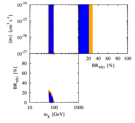
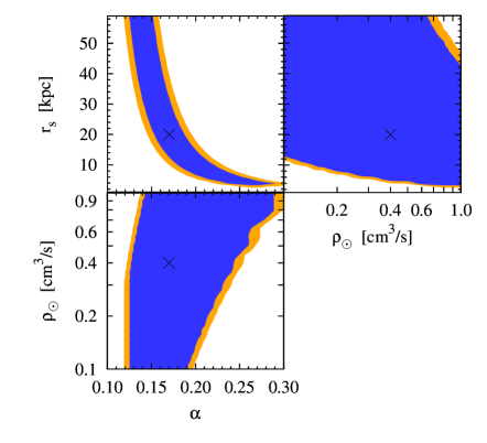
Figure 1: Fermi–LAT abilities to simultaneously constrain DM properties (left panel) and the Milky Way DM density distribution (right panel) after 5 years. We consider DM annihilation into a pure $b\bar{b}$ final state ($\text{BR}_{\tau(b)}=0$), $\langle\sigma v\rangle=3\times 10^{-26}$ cm³/s and $m_{\chi}=80$ GeV. For the DM density profile we consider an Einasto profile with $\rho_{\odot}=0.4$ GeV/cm³, $r_{s}=20$ kpc, $\alpha=0.17$ and $R_{\odot}=8.3$ kpc. The black crosses indicate the values of these parameters. In both panels, blue (orange) regions represent the 68% CL (90% CL) contours for 2 dof.

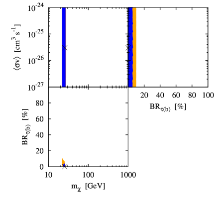
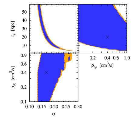
Figure 2: Fermi–LAT abilities to simultaneously constrain DM properties (left panel) and the Milky Way DM density distribution (right panel) after 5 years. Same as Fig. 1 but for $m_{\chi}=25$ GeV.

For the first four figures, Figs. 1–4, we consider an Einasto profile (Eq. (4)) with our default values for the local DM density and the Sun distance to the GC ($\rho_{\odot}=0.4$ GeV/cm³ and $R_{\odot}=8.3$ kpc) and we further set the other two parameters to $r_{s}=20$ kpc and $\alpha=0.17$. These values for the scale radius and the index $\alpha$ are the ones commonly assumed in studies of DM indirect detection. Moreover, this value of $\alpha$ approximately represents the mean value obtained from N-body simulations for dark halos with virial masses of the order of $10^{12}\,{\rm M}_{\odot}$ [118]. Concerning the DM particle properties, we assume DM annihilation into a pure $b\bar{b}$ final state and an annihilation cross section (times relative velocity) $\langle\sigma v\rangle=3\times 10^{-26}$ cm³/s. The left panels of the four figures show the results for pairs of DM properties after marginalizing with respect to the rest of the parameters and the right panels show the results for the parameters that describe the DM density profile.

In Fig. 1, we depict the Fermi–LAT reconstruction prospects after 5 years. The blue regions and the orange regions correspond to the 68% and 90% confidence level (CL) contours for 2 degrees of freedom (dof), respectively. However, note that there are very small differences between these contours, which is due to a very steep $\chi^{2}$.

From the left panel one can extract two important pieces of information. On one side, unlike what happens if the DM density profile is assumed to be known [61], in the present case the value of the annihilation cross section would remain completely unknown. This can be easily understood by the fact that by also fitting the DM density profile, the quantity $\rho_{\odot}^{2}\,\overline{J}$ is allowed to vary and along with $\langle\sigma v\rangle$, that quantity sets the normalization of the potential signal (see Eq. (1)). Thus, there is a clear degeneracy between them, which cannot be broken by the energy or angular binning of the signal. On the other hand, the capabilities for the reconstruction of the DM mass and annihilation channel do not substantially worsen with respect to the case of a known DM density profile (but with a single angular bin) [61]. This is clearly due to binning the signal both spatially and in energy, as there are more “data” points and the energy spectrum obviously depends on the DM mass and on the annihilation channel. Hence, the DM mass could be determined with a $\sim 25\%$ uncertainty and the branching ratio could simultaneously be constrained to be $\text{BR}_{\tau(b)}\lesssim 0.25$ at 90% CL (2 dof).

From the right panel of Fig. 1, one realizes that it could be possible to establish a strong correlation between $r_{s}$ and $\alpha$ at a high CL (note again that the $\chi^{2}$ is very steep). It is important to stress that this could be achieved by only using gamma-ray observations with no further constraints on the relevant parameters and basically thanks to the angular binning. There are also correlations among these parameters and $\rho_{\odot}$, although they are much weaker. Nevertheless, due to the degeneracy between $\rho_{\odot}^{2}\,\overline{J}$ and $\langle\sigma v\rangle$, it turns out that the actual values of the parameters that describe the DM density profile cannot be determined with only gamma-rays. Although being a very weak constraint, $\alpha$ could be found to lie in the range $\alpha=(0.12-0.30)$ at 90% CL (2 dof).

In Fig. 2 we show the corresponding results for the case of $m_{\chi}=25$ GeV. The same trends as in Fig. 1 are observed, although due to larger statistics, slightly better results would be obtained. We see that the DM mass could be determined with a $\sim 10\%$ uncertainty and simultaneously, the branching ratio could be constrained to be $\text{BR}_{\tau(b)}\lesssim 0.10$ at 90% CL (2 dof). In addition, the index $\alpha$ could be bounded to lie in the range $\alpha\simeq(0.13-0.27)$ at 90% CL (2 dof). We also note that the correlations between parameters get tighter, but the degeneracy between $\rho_{\odot}^{2}\,\overline{J}$ and $\langle\sigma v\rangle$ cannot be broken, which would prevent us from being able to determine neither the annihilation cross section nor the exact parameters that describe the DM density profile.

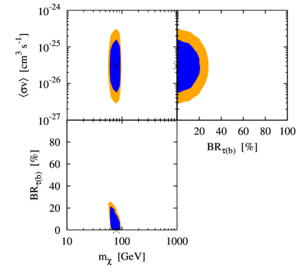
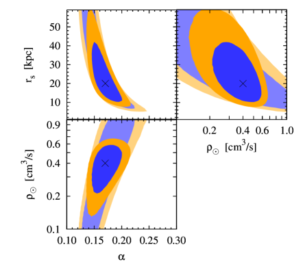
Figure 3: Fermi–LAT abilities to simultaneously constrain DM properties (left panel) and the Milky Way DM density distribution (right panel) after 5 years, with the addition of external information on $\boldsymbol{\rho_{\odot}}$ and $\boldsymbol{\langle\sigma v\rangle}$ (see text). Same parameters as in Fig. 1. In both panels, the dark (light) regions represent the case of $\sigma_{\log\langle\sigma v\rangle}=0.15$ and $\sigma_{\rho_{\odot}}=0.1\,\rho_{\odot}$ ($\sigma_{\rho_{\odot}}=0.5\,\rho_{\odot}$). As in Fig. 1, blue (orange) regions represent the 68% CL (90% CL) contours for 2 dof.

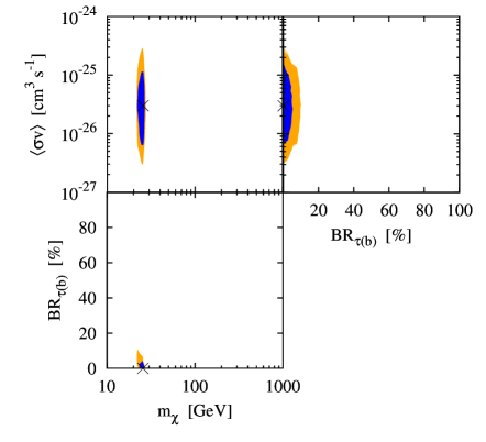
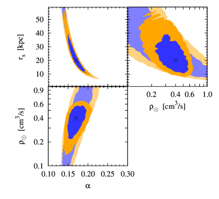
Figure 4: Fermi–LAT abilities to simultaneously constrain DM properties (left panel) and the Milky Way DM density distribution (right panel) after 5 years, with the addition of external information on $\boldsymbol{\rho_{\odot}}$ and $\boldsymbol{\langle\sigma v\rangle}$ (see text). Same as Fig. 3 but for $m_{\chi}=25$ GeV.

So far, we have shown results that could be obtained by just using gamma-ray observations. However, we already have some information about some of the parameters entering the fit, as the local DM density ($\rho_{\odot}$) [51, 52, 79, 137, 132, 138], and one would also hope that other parameters might be constrained in the future, as the annihilation cross section ($\langle\sigma v\rangle$) and the DM mass ($m_{\chi}$) [70, 71, 72, 73, 74, 75, 76, 77, 78, 79, 80, 81, 82, 83, 84, 85, 86, 87, 88, 89, 90, 91, 92, 93, 94, 95, 96, 97, 98, 99, 100, 101, 102, 103, 104, 105, 106, 107, 108]. In Figs. 3 and 4, we show how our knowledge about the structure of the Milky Way dark halo could be largely improved if we add to the gamma-ray analysis, constraints coming from other sources on $\rho_{\odot}$ and $\langle\sigma v\rangle$.

For the local DM density we will consider two different priors. On one side, we follow the common and conservative approach of assuming that it is determined within a factor of two and set a 50% error, $\sigma_{\rho_{\odot}}=0.5\,\rho_{\odot}$. On the other hand, we also consider a more optimistic constraint as recently obtained in different works [51, 132], $\sigma_{\rho_{\odot}}=0.1\,\rho_{\odot}$.

Concerning some of the DM properties, we will only set a prior on the annihilation cross section. Although there are good prospects of constraining the DM mass by using direct searches and collider experiments, we will not implement this potential constraint in what follows. As shown above, a gamma-ray observation could allow a quite good determination of the DM mass if the DM particle is relatively light ($m_{\chi}\lesssim 100$ GeV). Indeed, we have checked that a further external constraint on this parameter would not add substantial information. However, as also discussed above, there is a degeneracy between $\rho_{\odot}^{2}\,\overline{J}$ and $\langle\sigma v\rangle$, so in order to break it as much as possible, not only is the information on $\rho_{\odot}$ important, but a constraint on $\langle\sigma v\rangle$ is also needed. Hence, we assume that the annihilation cross section might be determined within an order of magnitude at $3\sigma$ with future collider data [98] and set a very optimistic prior $\sigma_{\log\langle\sigma v\rangle}=0.15$, where $\langle\sigma v\rangle$ is expressed in cm³/s. We note that a weaker constraint on this parameter would not improve significantly the results as compared to the case with no priors, so in this regard, information on both $\rho_{\odot}$ and $\langle\sigma v\rangle$ is crucial to reduce the allowed parameter space to determine the structure of the Milky Way DM halo.

In order to implement these priors, we add a penalty factor to the $\chi^{2}$ for each parameter (with Gaussian error), which takes into account the external information. The new $\chi^{2}$ reads

$$\chi^{2}_{\text{prior}}\left({\bf\theta}\right)=\sum_{j=1}^{10}\sum_{i=1}^{20}\frac{\left(S_{ij}\left({\bf\theta}\right)-S_{ij}^{\text{th}}\left({\bf\theta^{0}}\right)\right)^{2}}{(\sigma_{\rm stat})_{ij}^{2}+(\sigma_{\rm sys})_{ij}^{2}}+\left(\frac{\rho_{\odot}-\rho_{\odot}^{0}}{\sigma_{\rho_{\odot}}}\right)^{2}+\left(\frac{\log\langle\sigma v\rangle-\log\langle\sigma v\rangle^{0}}{\sigma_{\log\langle\sigma v\rangle}}\right)^{2}\leavevmode\nobreak\ ,$$ (8)

where again, in $\log\langle\sigma v\rangle$, $\langle\sigma v\rangle$ is expressed in cm³/s.

In Figs. 3 and 4 we assume the same parameters as in Figs. 1 and 2, respectively, but now we add the external information on $\rho_{\odot}$ and $\langle\sigma v\rangle$ we have just discussed. In both figures, the blue (orange) regions correspond to the 68% CL (90% CL) contours for 2 dof. In these figures, the case of our most optimistic set of priors ($\sigma_{\log\langle\sigma v\rangle}=0.15$ and $\sigma_{\rho_{\odot}}=0.1\,\rho_{\odot}$) is represented by the dark regions, whereas the slightly less optimistic case ($\sigma_{\log\langle\sigma v\rangle}=0.15$ and $\sigma_{\rho_{\odot}}=0.5\,\rho_{\odot}$) is depicted as the light regions.

In both figures, we see that there is no further improvement on the determination of the DM mass or the annihilation branching ratio, as gamma-rays do not provide more stringent constraints on $\langle\sigma v\rangle$ than what we assume to get from collider experiments or DM direct detection searches. Likewise, the “data” on gamma-rays do not add further information on the local DM density. Nevertheless, for the case of $m_{\chi}=80$ GeV (Fig. 3), the index $\alpha$ could be constrained to lie in the range $\alpha\simeq(0.13-0.22)$ and $\alpha\simeq(0.12-0.25)$ at 90% CL (2 dof) and for our most and less optimistic priors, respectively. Although modest, this could be an useful piece of information. On the other hand, $r_{s}$ could be only weakly constrained for the case with our most optimistic priors, $r_{s}\simeq(8-60)\leavevmode\nobreak\ \text{kpc}$ at 90% CL (2 dof).

Similar improvements are obtained for a lighter DM, as shown in Fig. 4 for $m_{\chi}=25$ GeV. Very small differences are found between the results for these two DM masses. The allowed range for the index $\alpha$ would turn out to be $\alpha\simeq(0.14-0.21)$ and $\alpha\simeq(0.13-0.23)$ at 90% CL (2 dof) and for our most and less optimistic priors, respectively. On the other hand, with our most optimistic priors, the allowed region for the scale radius would be $r_{s}\simeq(8-56)\leavevmode\nobreak\ \text{kpc}$ at 90% CL (2 dof).

5.2 Comparison with numerical simulations

The parametrization commonly used when studying the structural properties of DM halos by means of numerical N-body simulations is the NFW profile (Eq. (3)). Thus, in order to compare our findings with their results, we consider this parametrization in the next three figures.

In Figs. 5–7, we show the results for different values of the parameters that describe the DM halo (we again set $R_{\odot}=8.3$ kpc), that is the local DM density and the scale radius or equivalently, the virial mass and the concentration parameter. Indeed, for the sake of comparison with simulations, we show the results in the plane $(M_{\rm vir},c_{\rm vir})$ , after marginalizing with respect to the three DM particle parameters we study. However, we do not show here the prospects to constrain these parameters, as the results are very similar to those obtained for the Einasto profile and depicted in the left panels of Figs. 1–4. In the next figures, we assume the same DM mass, $m_{\chi}=25$ GeV and, as in Figs. 1–4, we consider DM annihilation into a pure $b\bar{b}$ final state and an annihilation cross section (times relative velocity) $\langle\sigma v\rangle=3\times 10^{-26}$ cm³/s.

The left panels of Figs. 5–7 show the capabilities of the Fermi–LAT experiment to reconstruct the halo properties after 5 years. For these panels no external priors are assumed, analogously to Figs. 1 and 2. As in the Einasto case, the blue and orange regions correspond to the 68% and 90% CL contours for 2 dof, respectively. Again, we see that there are very small differences between these contours due to a very steep $\chi^{2}$.

The right panels of Figs. 5–7 depict the results in the case of adding external information on $\rho_{\odot}$ and $\langle\sigma v\rangle$, as in Figs. 3 and 4. Likewise, the blue (orange) regions correspond to the 68% CL (90% CL) contours for 2 dof. In these panels, the case of our most optimistic set of priors ($\sigma_{\log\langle\sigma v\rangle}=0.15$ and $\sigma_{\rho_{\odot}}=0.1\,\rho_{\odot}$) is also represented by the dark regions, whereas we show the less optimistic case ($\sigma_{\log\langle\sigma v\rangle}=0.15$ and $\sigma_{\rho_{\odot}}=0.5\,\rho_{\odot}$) as the light regions.

In all three figures, in both panels, the red solid curves represent the mean value and $1\sigma$ scatter band of the concentration parameter obtained in numerical simulations (see Eq. (5) and discussion below). The central black dashed line indicates our default value for the local DM density, $\rho_{\odot}=0.4$ GeV/cm³, whereas the lower black dashed line indicate $\rho_{\odot}=0.2$ GeV/cm³ and the upper one $\rho_{\odot}=0.6$ GeV/cm³.

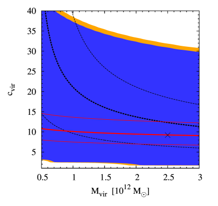
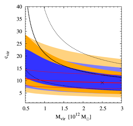
Figure 5: Fermi–LAT abilities to constrain the Milky Way DM density distribution after 5 years (keeping correlations with DM particle properties). We consider DM annihilation into a pure $b\bar{b}$ final state ($\text{BR}_{\tau(b)}=0$), $\langle\sigma v\rangle=3\times 10^{-26}$ cm³/s and $m_{\chi}=25$ GeV. We assume a NFW profile, $\rho_{\odot}=0.3$ GeV/cm³, $R_{\odot}=8.3$ kpc and the relation in Eq. (5) ($c_{\rm vir}=9.2$, $r_{s}=38.6$ kpc and $M_{\rm vir}=2.5\times 10^{12}\,{\rm M}_{\odot}$). The black crosses indicate the corresponding values in the $(M_{\rm vir},c_{\rm vir})$ plane. In both panels, blue (orange) regions represent the 68% CL (90% CL) contours for 2 dof. The left panels show the case with no external priors and in the right panels two external priors are adopted: $\sigma_{\log\langle\sigma v\rangle}=0.15$ and $\sigma_{\rho_{\odot}}=0.1\,\rho_{\odot}$ for the dark regions and $\sigma_{\log\langle\sigma v\rangle}=0.15$ and $\sigma_{\rho_{\odot}}=0.5\,\rho_{\odot}$ for the light contours. Red solid lines indicate the mean concentration parameter obtained from numerical simulations [49] and the $1\sigma$ scatter band ($\sigma_{\ln c_{\rm vir}}=0.3$); black dashed lines indicate bottom-up $\rho_{\odot}=0.2$ GeV/cm³, $0.4$ GeV/cm³ and $0.6$ GeV/cm³.

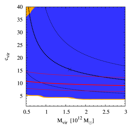
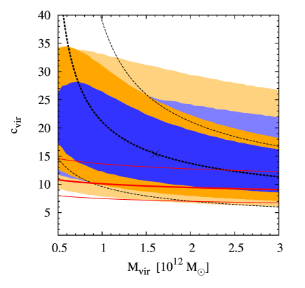
Figure 6: Fermi–LAT abilities to constrain the Milky Way DM density distribution after 5 years (keeping correlations with DM particle properties). Same as Fig. 7, but for $\rho_{\odot}=0.4$ GeV/cm³ and $r_{s}=20$ kpc ($c_{\rm vir}=15.2$ and $M_{\rm vir}=1.6\times 10^{12}\,{\rm M}_{\odot}$).

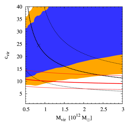
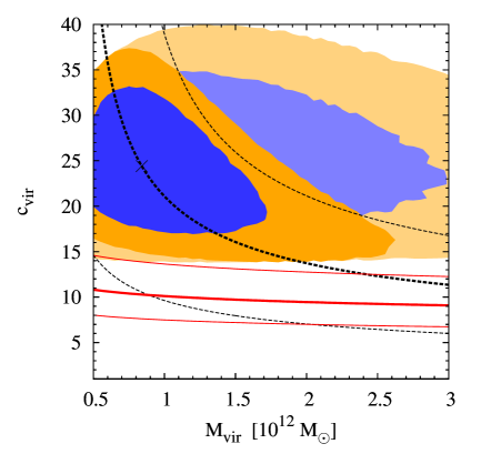
Figure 7: Fermi–LAT abilities to constrain the Milky Way DM density distribution after 5 years (keeping correlations with DM particle properties). Same as Fig. 7, but for $\rho_{\odot}=0.4$ GeV/cm³ and $M_{\rm dh}=4.0\times 10^{11}\,{\rm M}_{\odot}$ ($r_{s}=10$ kpc, $c_{\rm vir}=24.4$ and $M_{\rm vir}=8.4\times 10^{11}\,{\rm M}_{\odot}$).

We first consider in Fig. 5 the case of $\rho_{\odot}=0.3$ GeV/cm³ and impose the relation $M_{\rm vir}-c_{\rm vir}$ for the mean obtained in numerical simulations [49] (see Eq. (5)). In this way, the two-parameter profile gets reduced to a one-parameter parametrization. Thus, a local DM density  $\rho_{\odot}=0.3$ GeV/cm³ and Eq. (5) imply $M_{\rm vir}=2.5\times 10^{12}\,{\rm M}_{\odot}$ and $c_{\rm vir}=9.2$. The scale radius is predicted to be $r_{s}=38.6$ kpc, which is much larger than the value of 20 kpc commonly used in the literature of DM indirect detection. As we see from Fig. 5, the gamma-ray data alone would not be able to set any significant constraint on the DM density profile. Moreover, although adding external information on $\rho_{\odot}$ and $\langle\sigma v\rangle$ would substantially reduce the allowed parameter space, yet a large fraction would still be unconstrained even in the most optimistic of our cases. In particular, no bounds on the virial mass could be set with this technique.

In general, the larger the scale radius (the smaller the concentration parameter) the lower the potential signal from DM annihilations. In Fig. 6 we consider $\rho_{\odot}=0.4$ GeV/cm³ and $r_{s}=20$ kpc, which as mentioned above, is the common value used in works related to indirect DM detection. In this case, $M_{\rm vir}=1.6\times 10^{12}\,{\rm M}_{\odot}$ and $c_{\rm vir}=15.2$. Let us note that this value for the scale radius implies a concentration parameter much larger  than what is obtained, for $M_{\rm vir}\sim 10^{12}\,{\rm M}_{\odot}$, for the mean in numerical simulations, $c_{\rm vir}\sim 9-11$, and it is even away from the $1\sigma$ scatter. Thus, although certainly plausible, its choice is not really justified by the value of the mean of the concentration parameter obtained in numerical simulations. It is interesting to notice, though, that these parameters are very close to those obtained in a very recent estimate [132]. In the left panel of Fig. 6, we see that gamma-ray data alone would not be able to offer any information on the DM density distribution in this case either. The addition of external constraints would allow to substantially restrict the allowed parameter space, as can be seen from the right panel. However, only limited information could be extracted, even in the case of our most optimistic priors. At 90% CL (2 dof), the allowed parameter space would be compatible with the mean obtained in numerical simulations.

On the other hand, in Fig. 7 we use a recent estimate of the dark halo mass within the innermost 60 kpc of the Milky Way [128], which predicts a lower mass than other works, and we assume $M_{\rm dh}(60)=4.0\times 10^{11}\,{\rm M}_{\odot}$. By considering a local DM density given by our default value, $\rho_{\odot}=0.4$ GeV/cm³, this implies a scale radius much smaller, $r_{s}=10$ kpc, than what is usually assumed and a concentration parameter correspondingly much larger, $c_{\rm vir}=24.4$, than what is predicted from N-body simulations for halos with virial masses about $10^{12}\,{\rm M}_{\odot}$ (cf. Eq. (5)). From the left panel, we see that a large part of the $1\sigma$ scatter band obtained by numerical simulations would be disfavored by such a measurement with only gamma-rays. This trend is further accentuated if external information on $\rho_{\odot}$ and $\langle\sigma v\rangle$ is available. In that case, even with our less optimistic priors, predictions of numerical simulations would be disfavored at more than 90% CL, as can be seen from the right panel. Hence, in this situation a Fermi–LAT detection of DM would point out that a revision of our current understanding of halo clustering and evolution is mandatory, perhaps due to the influence of baryons, which are usually not included in the simulations.

All in all, we see that numerical simulations tend to predict a mean concentration parameter which typically implies low statistics in a gamma-ray experiment and thus, extracting information about the DM density distribution would become a very challenging task in this case. In contrast, typical values for the DM local density imply large values of the concentration parameter, which decrease with the virial mass. Hence, in order to avoid strong conflict with numerical simulations, a virial mass in the high-mass side of the allowed interval would be needed. However, a recent determination of the DM halo mass within the innermost 60 kpc [128] points to a low virial mass, which would imply a large concentration parameter, in clear conflict with numerical simulations (for commonly inferred values of the DM local density), but with much more promising prospects to constrain the halo density distribution with a gamma-ray experiment like Fermi–LAT.

6 Conclusions

During the last two decades, the progress in high resolution N-body simulations has led to the discovery of a universal density profile for CDM halos [17, 18, 111, 33, 115, 116, 117, 118] that can be parametrized in analytical forms containing very few parameters. However, these prescriptions only represent the mean results for all simulated halos, but cannot describe the large scatter that is found [35, 36, 37, 38, 39, 40]. Moreover, these simulations do not usually include the effect of baryons, which could significantly change the picture [167, 168, 169, 170, 171, 172, 173, 174, 175]. Hence, for the particular case of our Milky Way, these mean values do not necessarily describe its CDM halo.

This is a very important issue, as the predictions for the potential signals for the astrophysical detection of DM critically depend on the structure of the Milky Way halo. Indeed, several approaches have been proposed to determine DM particle properties by using future indirect WIMP DM-induced signals of gamma-rays or neutrinos, direct detection searches, collider information or their combination [57, 58, 59, 60, 61, 62, 63, 64, 65, 66, 67, 68, 69, 70, 71, 72, 73, 74, 75, 76, 77, 78, 79, 80, 81, 82, 83, 84, 85, 86, 87, 88, 89, 90, 91, 92, 93, 94, 95, 96, 97, 98, 99, 100, 101, 102, 103, 104, 105, 106, 107, 108]. All these measurements would be complementary and would constitute an important step toward the identification of the particle nature of DM. However, without a better knowledge of the Milky Way DM density profile, large uncertainties would be present. This, in the case of a positive signal, would make the task of constraining DM properties a much more challenging one.

In the case of gamma-ray studies, although different profiles have been considered in the literature, a single DM density profile is commonly assumed to determine the capabilities of gamma-ray experiments to extract some DM properties [57, 58, 59, 60, 61, 62], and thus in general, the obtained results are too optimistic. Here, we have studied the effect these astrophysical uncertainties would have on the determination of some DM particle properties, as annihilation cross section, mass and branching ratio into dominant annihilation channels. Conversely, gamma-ray searches could also be used to learn about the structure of the Milky Way DM halo, as a complementary tool to other type of observational data that study the gravitational effect caused by the presence of DM.

In this work, we have studied the capabilities of the Fermi–LAT instrument on board of the Fermi mission [53] to tackle these issues and consider the potential gamma-ray signal in a squared region with a side of $20^{\circ}$ around the GC ($|l|,|b|<10^{\circ}$) after 5 years of data taking. In order to model the relevant gamma-ray backgrounds, we use the numerical code GALPROP [54] and the latest Fermi–LAT observations [55, 56].

In two introductory sections (Sections 2 and 3) we review the main components of the gamma-ray emission from DM annihilation in the GC, and critically discuss the current knowledge of the parameters involved in the description of the (smooth) Milky DM density profile. Then, in Section 4 we describe our modeling of the Fermi-LAT experiment and the ingredients of the analysis we perform. Finally, in Section 5, we present the results of our paper. First, we consider an Einasto profile and study the Fermi-LAT capabilities to simultaneously constrain DM particle properties and the parameters that describe the DM density profile. We do so for two DM masses, $m_{\chi}=80$ GeV (Fig. 1) and $m_{\chi}=25$ GeV (Fig. 2). These results could be compared to those of Ref. [61], where a particular DM density profile was assumed to perform the fits, but with a single angular bin. In addition, we also consider the improvement in these results when external information on $\langle\sigma v\rangle$ and $\rho_{\odot}$ is included (Figs. 3 and 4). In the last part of this work, we focus on the determination of the parameters that describe the DM density profile. In order to compare our results to the relations obtained in numerical simulations, we consider a NFW profile, study different sets of values for the parameters and plot the results in the $(M_{\rm vir},c_{\rm vir})$ plane (Figs. 5–7). The parameters and relevant information for each of the figures are summarized in Table 1.

In summary, and baring in mind the difficulties of all experiments that aim to detect DM to distinguish that signal from any other possible backgrounds, our study shows the Fermi–LAT capabilities to simultaneously constrain DM particle properties and the Milky Way DM density distribution. Along these lines, we have tried to point out some important issues that should be taken into account in indirect searches when a potential DM signal is detected.

References

- [1] G. Jungman, M. Kamionkowski, and K. Griest, “Supersymmetric dark matter”, Phys. Rept. 267 (1996) 195, arXiv:hep-ph/9506380.
- [2] L. Bergström, “Non-baryonic dark matter: Observational evidence and detection methods”, Rept. Prog. Phys. 63 (2000) 793, arXiv:hep-ph/0002126.
- [3] C. Muñoz, “Dark matter detection in the light of recent experimental results”, Int. J. Mod. Phys. A19 (2004) 3093, arXiv:hep-ph/0309346.
- [4] G. Bertone, D. Hooper, and J. Silk, “Particle dark matter: Evidence, candidates and constraints”, Phys. Rept. 405 (2005) 279, arXiv:hep-ph/0404175.
- [5] G. Bertone, ed., Particle Dark Matter: Observations, Models and Searches. Cambridge University Press, 2010.
- [6] SDSS Collaboration, M. Tegmark et al., “Cosmological Constraints from the SDSS Luminous Red Galaxies”, Phys. Rev. D74 (2006) 123507, arXiv:astro-ph/0608632.
- [7] WMAP Collaboration, E. Komatsu et al., “Five-Year Wilkinson Microwave Anisotropy Probe (WMAP) Observations:Cosmological Interpretation”, Astrophys. J. Suppl. 180 (2009) 330, arXiv:0803.0547 [astro-ph].
- [8] WMAP Collaboration, E. Komatsu et al., “Seven-Year Wilkinson Microwave Anisotropy Probe (WMAP) Observations: Cosmological Interpretation”, Astrophys. J. Suppl. 192 (2011) 18, arXiv:1001.4538 [astro-ph.CO].
- [9] L. Bergström, “Dark Matter Candidates”, New J. Phys. 11 (2009) 105006, arXiv:0903.4849 [hep-ph].
- [10] A. Birkedal, A. Noble, M. Perelstein, and A. Spray, “Little Higgs dark matter”, Phys. Rev. D74 (2006) 035002, arXiv:hep-ph/0603077.
- [11] D. Hooper and S. Profumo, “Dark matter and collider phenomenology of universal extra dimensions”, Phys. Rept. 453 (2007) 29, arXiv:hep-ph/0701197.
- [12] S. D. M. White and M. J. Rees, “Core condensation in heavy halos: A Two stage theory for galaxy formation and clusters”, Mon. Not. Roy. Astron. Soc. 183 (1978) 341.
- [13] G. R. Blumenthal, S. M. Faber, J. R. Primack, and M. J. Rees, “Formation of galaxies and large-scale structure with cold dark matter”, Nature 311 (1984) 517.
- [14] S. D. M. White and C. S. Frenk, “Galaxy formation through hierarchical clustering”, Astrophys. J. 379 (1991) 52.
- [15] H. J. Mo, S. Mao, and S. D. M. White, “The Formation of Galactic Disks”, Mon. Not. Roy. Astron. Soc. 295 (1998) 319, arXiv:astro-ph/9707093.
- [16] J. E. Gunn, “Massive galactic halos. I - Formation and evolution”, Astrophys. J. 218 (1977) 592.
- [17] J. F. Navarro, C. S. Frenk, and S. D. M. White, “The Structure of Cold Dark Matter Halos”, Astrophys. J. 462 (1996) 563, arXiv:astro-ph/9508025.
- [18] J. F. Navarro, C. S. Frenk, and S. D. M. White, “A Universal Density Profile from Hierarchical Clustering”, Astrophys. J. 490 (1997) 493, arXiv:astro-ph/9611107.
- [19] A. Burkert, “The Structure of dark matter halos in dwarf galaxies”, IAU Symp. 171 (1996) 175, arXiv:astro-ph/9504041.
- [20] B. Moore, T. R. Quinn, F. Governato, J. Stadel, and G. Lake, “Cold collapse and the core catastrophe”, Mon. Not. Roy. Astron. Soc. 310 (1999) 1147, arXiv:astro-ph/9903164.
- [21] S. Ghigna et al., “Density profiles and substructure of dark matter halos: converging results at ultra-high numerical resolution”, Astrophys. J. 544 (2000) 616, arXiv:astro-ph/9910166.
- [22] T. Fukushige and J. Makino, “Origin of Cusp in Dark Matter Halo”, Astrophys. J. 477 (1997) L9, arXiv:astro-ph/9610005.
- [23] K. Subramanian, R. Cen, and J. P. Ostriker, “The structure of dark matter halos in hierarchical clustering theories”, Astrophys. J. 538 (2000) 528, arXiv:astro-ph/9909279.
- [24] T. Fukushige and J. Makino, “Structure of Dark Matter Halos From Hierarchical Clustering”, Astrophys. J. 557 (2001) 533, arXiv:astro-ph/0008104.
- [25] A. Klypin, A. V. Kravtsov, J. Bullock, and J. Primack, “Resolving the structure of cold dark matter halos”, Astrophys. J. 554 (2001) 903, arXiv:astro-ph/0006343.
- [26] J. E. Taylor and J. F. Navarro, “The Phase-Space Density Profiles of Cold Dark Matter Halos”, Astrophys. J. 563 (2001) 483, arXiv:astro-ph/0104002.
- [27] C. Power et al., “The Inner Structure of LambdaCDM Halos I: A Numerical Convergence Study”, Mon. Not. Roy. Astron. Soc. 338 (2003) 14, arXiv:astro-ph/0201544.
- [28] M. Ricotti, “Dependence of the Inner DM Profile on the Halo Mass”, Mon. Not. Roy. Astron. Soc. 344 (2003) 1237, arXiv:astro-ph/0212146.
- [29] T. Fukushige, A. Kawai, and J. Makino, “Structure of Dark Matter Halos From Hierarchical Clustering. III. Shallowing of The Inner Cusp”, Astrophys. J. 606 (2004) 625, arXiv:astro-ph/0306203.
- [30] J. Diemand, B. Moore, and J. Stadel, “Convergence and scatter of cluster density profiles”, Mon. Not. Roy. Astron. Soc. 353 (2004) 624, arXiv:astro-ph/0402267.
- [31] G. Gentile, P. Salucci, U. Klein, D. Vergani, and P. Kalberla, “The cored distribution of dark matter in spiral galaxies”, Mon. Not. Roy. Astron. Soc. 351 (2004) 903, arXiv:astro-ph/0403154.
- [32] P. Salucci et al., “The universal rotation curve of spiral galaxies. II: The dark matter distribution out to the virial radius”, Mon. Not. Roy. Astron. Soc. 378 (2007) 41, arXiv:astro-ph/0703115.
- [33] J. F. Navarro et al., “The Inner Structure of LambdaCDM Halos III: Universality and Asymptotic Slopes”, Mon. Not. Roy. Astron. Soc. 349 (2004) 1039, arXiv:astro-ph/0311231.
- [34] J. Einasto, “On the Construction of a Composite Model for the Galaxy and on the Determination of the System of Galactic Parameters”, Trudy Inst. Astrofiz. Alma-Ata 51 (1965) 87.
- [35] Y. P. Jing, “The density profile of equilibrium and non-equilibrium dark matter halos”, Astrophys. J. 535 (2000) 30, arXiv:astro-ph/9901340.
- [36] J. S. Bullock et al., “Profiles of dark haloes: evolution, scatter, and environment”, Mon. Not. Roy. Astron. Soc. 321 (2001) 559, arXiv:astro-ph/9908159.
- [37] R. H. Wechsler, J. S. Bullock, J. R. Primack, A. V. Kravtsov, and A. Dekel, “Concentrations of Dark Halos from their Assembly Histories”, Astrophys. J. 568 (2002) 52, arXiv:astro-ph/0108151.
- [38] V. Avila-Reese, P. Colin, S. Gottlober, C. Firmani, and C. Maulbetsch, “The dependence on environment of Cold Dark Matter Halo properties”, Astrophys. J. 634 (2005) 51–69, arXiv:astro-ph/0508053.
- [39] A. V. Macciò et al., “Concentration, Spin and Shape of Dark Matter Haloes: Scatter and the Dependence on Mass and Environment”, Mon. Not. Roy. Astron. Soc. 378 (2007) 55, arXiv:astro-ph/0608157.
- [40] A. V. Macciò, A. A. Dutton, and F. C. v. d. Bosch, “Concentration, Spin and Shape of Dark Matter Haloes as a Function of the Cosmological Model: WMAP1, WMAP3 and WMAP5 results”, Mon. Not. Roy. Astron. Soc. 391 (2008) 1940, arXiv:0805.1926 [astro-ph].
- [41] V. R. Eke, J. F. Navarro, and M. Steinmetz, “The Power Spectrum Dependence of Dark Matter Halo Concentrations”, Astrophys. J. 554 (2001) 114, arXiv:astro-ph/0012337.
- [42] D. Zhao, H. Mo, Y. Jing, and G. Boerner, “The Growth and Structure of Dark Matter Haloes”, Mon. Not. Roy. Astron. Soc. 339 (2003) 12, arXiv:astro-ph/0204108.
- [43] D.-H. Zhao, Y. P. Jing, H. J. Mo, and G. Borner, “Mass and Redshift Dependence of Dark Halo Structure”, Astrophys. J. 597 (2003) L9, arXiv:astro-ph/0309375.
- [44] A. F. Neto et al., “The statistics of LCDM Halo Concentrations”, Mon. Not. Roy. Astron. Soc. 381 (2007) 1450, arXiv:0706.2919 [astro-ph].
- [45] L. Gao et al., “The redshift dependence of the structure of massive LCDM halos”, Mon. Not. Roy. Astron. Soc. 387 (2008) 536, arXiv:0711.0746 [astro-ph].
- [46] A. R. Duffy, J. Schaye, S. T. Kay, and C. Dalla Vecchia, “Dark matter halo concentrations in the WMAP5 cosmology”, Mon. Not. Roy. Astron. Soc. 390 (2008) l64, arXiv:0804.2486 [astro-ph].
- [47] D. H. Zhao, Y. P. Jing, H. J. Mo, and G. Boerner, “Accurate universal models for the mass accretion histories and concentrations of dark matter halos”, Astrophys. J. 707 (2009) 354, arXiv:0811.0828 [astro-ph].
- [48] A. Klypin, S. Trujillo-Gómez, and J. Primack, “Dark Matter halos and galaxies in the standard cosmological model: Results from the Bolshoi simulation”, Astrophys. J. 740 (2011) 102, arXiv:1002.3660 [astro-ph.CO].
- [49] J. C. Muñoz-Cuartas, A. V. Macciò, S. Gottlober, and A. A. Dutton, “The Redshift Evolution of LCDM Halo Parameters: Concentration, Spin, and Shape”, Mon. Not. Roy. Astron. Soc. 411 (2011) 584, arXiv:1007.0438 [astro-ph.CO].
- [50] M. Boylan-Kolchin, V. Springel, S. D. M. White, and A. Jenkins, “There’s no place like home? Statistics of Milky Way-mass dark matter halos”, Mon. Not. Roy. Astron. Soc. 406 (2010) 896, arXiv:0911.4484 [astro-ph.CO].
- [51] R. Catena and P. Ullio, “A novel determination of the local dark matter density”, JCAP 1008 (2010) 004, arXiv:0907.0018 [astro-ph.CO].
- [52] M. Weber and W. de Boer, “Determination of the Local Dark Matter Density in our Galaxy”, Astron. Astrophys. 509 (2010) A25, arXiv:0910.4272 [astro-ph.CO].
- [53] Fermi-LAT Collaboration, W. B. Atwood et al., “The Large Area Telescope on the Fermi Gamma-ray Space Telescope Mission”, Astrophys. J. 697 (2009) 1071, arXiv:0902.1089 [astro-ph.IM].
- [54] A. W. Strong and I. V. Moskalenko, “Propagation of cosmic-ray nucleons in the Galaxy”, Astrophys. J. 509 (1998) 212, arXiv:astro-ph/9807150.
- [55] Fermi-LAT Collaboration, A. A. Abdo et al., “Fermi Large Area Telescope First Source Catalog”, Astrophys. J. Supp. 188 (2010) 405, arXiv:1002.2280 [astro-ph.HE].
- [56] Fermi-LAT Collaboration, A. A. Abdo et al., “The Spectrum of the Isotropic Diffuse Gamma-Ray Emission Derived From First-Year Fermi Large Area Telescope Data”, Phys. Rev. Lett. 104 (2010) 101101, arXiv:1002.3603 [astro-ph.HE].
- [57] S. Dodelson, D. Hooper, and P. D. Serpico, “Extracting the Gamma Ray Signal from Dark Matter Annihilation in the Galactic Center Region”, Phys. Rev. D77 (2008) 063512, arXiv:0711.4621 [astro-ph].
- [58] N. Bernal, A. Goudelis, Y. Mambrini, and C. Muñoz, “Determining the WIMP mass using the complementarity between direct and indirect searches and the ILC”, JCAP 0901 (2009) 046, arXiv:0804.1976 [hep-ph].
- [59] N. Bernal, “WIMP mass from direct, indirect dark matter detection experiments and colliders: A complementary and model- independent approach”, arXiv:0805.2241 [hep-ph].
- [60] T. E. Jeltema and S. Profumo, “Fitting the Gamma-Ray Spectrum from Dark Matter with DMFIT: GLAST and the Galactic Center Region”, JCAP 0811 (2008) 003, arXiv:0808.2641 [astro-ph].
- [61] N. Bernal and S. Palomares-Ruiz, “Constraining Dark Matter Properties with Gamma-Rays from the Galactic Center with Fermi-LAT”, arXiv:1006.0477 [astro-ph.HE].
- [62] N. Bernal, “Reconstructing Dark Matter Properties via Gamma-Rays with Fermi-LAT”, arXiv:1012.0217 [astro-ph.HE].
- [63] S. Palomares-Ruiz and J. M. Siegal-Gaskins, “Annihilation vs. Decay: Constraining dark matter properties from a gamma-ray detection”, JCAP 1007 (2010) 023, arXiv:1003.1142 [astro-ph.CO].
- [64] S. Palomares-Ruiz and J. M. Siegal-Gaskins, “Annihilation vs. Decay: Constraining Dark Matter Properties from a Gamma-Ray Detection in Dwarf Galaxies”, arXiv:1012.2335 [astro-ph.CO].
- [65] J. Edsjö and P. Gondolo, “WIMP mass determination with neutrino telescopes”, Phys. Lett. B357 (1995) 595, arXiv:hep-ph/9504283.
- [66] M. Cirelli et al., “Spectra of neutrinos from dark matter annihilations”, Nucl. Phys. B727 (2005) 99, arXiv:hep-ph/0506298.
- [67] O. Mena, S. Palomares-Ruiz, and S. Pascoli, “Reconstructing WIMP properties with neutrino detectors”, Phys. Lett. B664 (2008) 92, arXiv:0706.3909 [hep-ph].
- [68] S. K. Agarwalla, M. Blennow, E. F. Martinez, and O. Mena, “Neutrino Probes of the Nature of Light Dark Matter”, JCAP 1109 (2011) 004, arXiv:1105.4077 [hep-ph].
- [69] C. R. Das, O. Mena, S. Palomares-Ruiz, and S. Pascoli, “Determining the dark matter mass with DeepCore”, arXiv:1110.5095 [hep-ph].
- [70] J. D. Lewin and P. F. Smith, “Review of mathematics, numerical factors, and corrections for dark matter experiments based on elastic nuclear recoil”, Astropart. Phys. 6 (1996) 87.
- [71] J. R. Primack, D. Seckel, and B. Sadoulet, “Detection of Cosmic Dark Matter”, Ann. Rev. Nucl. Part. Sci. 38 (1988) 751.
- [72] A. M. Green, “Determining the WIMP mass using direct detection experiments”, JCAP 0708 (2007) 022, arXiv:hep-ph/0703217.
- [73] G. Bertone, D. G. Cerdeño, J. I. Collar, and B. C. Odom, “WIMP identification through a combined measurement of axial and scalar couplings”, Phys. Rev. Lett. 99 (2007) 151301, arXiv:0705.2502 [astro-ph].
- [74] C.-L. Shan and M. Drees, “Determining the WIMP Mass from Direct Dark Matter Detection Data”, arXiv:0710.4296 [hep-ph].
- [75] M. Drees and C.-L. Shan, “Model-Independent Determination of the WIMP Mass from Direct Dark Matter Detection Data”, JCAP 0806 (2008) 012, arXiv:0803.4477 [hep-ph].
- [76] A. M. Green, “Determining the WIMP mass from a single direct detection experiment, a more detailed study”, JCAP 0807 (2008) 005, arXiv:0805.1704 [hep-ph].
- [77] M. Beltrán, D. Hooper, E. W. Kolb, and Z. C. Krusberg, “Deducing the nature of dark matter from direct and indirect detection experiments in the absence of collider signatures of new physics”, Phys. Rev. D80 (2009) 043509, arXiv:0808.3384 [hep-ph].
- [78] C.-L. Shan, “Determining the Mass of Dark Matter Particles with Direct Detection Experiments”, New J. Phys. 11 (2009) 105013, arXiv:0903.4320 [hep-ph].
- [79] L. E. Strigari and R. Trotta, “Reconstructing WIMP Properties in Direct Detection Experiments Including Galactic Dark Matter Distribution Uncertainties”, JCAP 0911 (2009) 019, arXiv:0906.5361 [astro-ph.HE].
- [80] A. H. G. Peter, “Getting the astrophysics and particle physics of dark matter out of next-generation direct detection experiments”, Phys. Rev. D81 (2010) 087301, arXiv:0910.4765 [astro-ph.CO].
- [81] Y.-T. Chou and C.-L. Shan, “Effects of Residue Background Events in Direct Dark Matter Detection Experiments on the Determination of the WIMP Mass”, JCAP 1008 (2010) 014, arXiv:1003.5277 [hep-ph].
- [82] C.-L. Shan, “Effects of Residue Background Events in Direct Dark Matter Detection Experiments on the Reconstruction of the Velocity Distribution Function of Halo WIMPs”, JCAP 1006 (2010) 029, arXiv:1003.5283 [astro-ph.HE].
- [83] P. J. Fox, G. D. Kribs, and T. M. P. Tait, “Interpreting Dark Matter Direct Detection Independently of the Local Velocity and Density Distribution”, Phys. Rev. D83 (2011) 034007, arXiv:1011.1910 [hep-ph].
- [84] C. Kelso and D. Hooper, “Prospects For Identifying Dark Matter With CoGeNT”, JCAP 1102 (2011) 002, arXiv:1011.3076 [hep-ph].
- [85] L. Bergström, T. Bringmann, and J. Edsjö, “Complementarity of direct dark matter detection and indirect detection through gamma-rays”, Phys.Rev. D83 (2011) 045024, arXiv:1011.4514 [hep-ph].
- [86] M. Pato et al., “Complementarity of Dark Matter Direct Detection Targets”, Phys. Rev. D83 (2011) 083505, arXiv:1012.3458 [astro-ph.CO].
- [87] J. Billard, F. Mayet, and D. Santos, “Markov Chain Monte Carlo analysis to constrain Dark Matter properties with directional detection”, Phys. Rev. D83 (2011) 075002, arXiv:1012.3960 [astro-ph.CO].
- [88] C.-L. Shan, “Estimating the Spin-Independent WIMP-Nucleon Coupling from Direct Dark Matter Detection Data”, arXiv:1103.0481 [hep-ph].
- [89] C.-L. Shan, “Determining Ratios of WIMP-Nucleon Cross Sections from Direct Dark Matter Detection Data”, JCAP 1107 (2011) 005, arXiv:1103.0482 [hep-ph].
- [90] M. Drees et al., “Scrutinizing LSP dark matter at the LHC”, Phys. Rev. D63 (2001) 035008, arXiv:hep-ph/0007202.
- [91] G. Polesello and D. R. Tovey, “Constraining SUSY dark matter with the ATLAS detector at the LHC”, JHEP 05 (2004) 071, arXiv:hep-ph/0403047.
- [92] M. Battaglia, I. Hinchliffe, and D. Tovey, “Cold dark matter and the LHC”, J. Phys. G30 (2004) R217, arXiv:hep-ph/0406147.
- [93] B. C. Allanach, G. Bélanger, F. Boudjema, and A. Pukhov, “Requirements on collider data to match the precision of WMAP on supersymmetric dark matter”, JHEP 12 (2004) 020, arXiv:hep-ph/0410091.
- [94] LHC/LC Study Group Collaboration, G. Weiglein et al., “Physics interplay of the LHC and the ILC”, Phys. Rept. 426 (2006) 47, arXiv:hep-ph/0410364.
- [95] A. Birkedal et al., “Testing cosmology at the ILC”, arXiv:hep-ph/0507214.
- [96] T. Moroi and Y. Shimizu, “Supersymmetric heavy Higgses at e+ e- linear collider and dark-matter physics”, Phys. Rev. D72 (2005) 115012, arXiv:hep-ph/0509196.
- [97] M. M. Nojiri, G. Polesello, and D. R. Tovey, “Constraining dark matter in the MSSM at the LHC”, JHEP 03 (2006) 063, arXiv:hep-ph/0512204.
- [98] E. A. Baltz, M. Battaglia, M. E. Peskin, and T. Wizansky, “Determination of dark matter properties at high-energy colliders”, Phys. Rev. D74 (2006) 103521, arXiv:hep-ph/0602187.
- [99] R. L. Arnowitt et al., “Indirect measurements of the stau - neutralino 1(0) mass difference and mSUGRA in the co-annihilation region of mSUGRA models at the LHC”, Phys. Lett. B649 (2007) 73, arXiv:hep-ph/0608193.
- [100] W. S. Cho, K. Choi, Y. G. Kim, and C. B. Park, “Gluino Stransverse Mass”, Phys. Rev. Lett. 100 (2008) 171801, arXiv:0709.0288 [hep-ph].
- [101] R. L. Arnowitt et al., “Determining the Dark Matter Relic Density in the mSUGRA Stau-Neutralino Co-Annhiliation Region at the LHC”, Phys. Rev. Lett. 100 (2008) 231802, arXiv:0802.2968 [hep-ph].
- [102] G. Bélanger, O. Kittel, S. Kraml, H. U. Martyn, and A. Pukhov, “Neutralino relic density from ILC measurements in the CPV MSSM”, Phys. Rev. D78 (2008) 015011, arXiv:0803.2584 [hep-ph].
- [103] W. S. Cho, K. Choi, Y. G. Kim, and C. B. Park, “M-assisted on-shell reconstruction of missing momenta and its application to spin measurement at the LHC”, Phys. Rev. D79 (2009) 031701, arXiv:0810.4853 [hep-ph].
- [104] H. Baer, E.-K. Park, and X. Tata, “Collider, direct and indirect detection of supersymmetric dark matter”, New J. Phys. 11 (2009) 105024, arXiv:0903.0555 [hep-ph].
- [105] D. Feldman, K. Freese, P. Nath, B. D. Nelson, and G. Peim, “Predictive Signatures of Supersymmetry: Measuring the Dark Matter Mass and Gluino Mass with Early LHC data”, Phys. Rev. D84 (2011) 015007, arXiv:1102.2548 [hep-ph].
- [106] J. L. Bourjaily and G. L. Kane, “What is the cosmological significance of a discovery of wimps at colliders or in direct experiments?”, arXiv:hep-ph/0501262.
- [107] B. Altunkaynak, M. Holmes, and B. D. Nelson, “Solving the LHC Inverse Problem with Dark Matter Observations”, JHEP 10 (2008) 013, arXiv:0804.2899 [hep-ph].
- [108] G. Bertone, D. G. Cerdeño, M. Fornasa, R. R. de Austri, and R. Trotta, “Identification of Dark Matter particles with LHC and direct detection data”, Phys. Rev. D82 (2010) 055008, arXiv:1005.4280 [hep-ph].
- [109] J. Diemand, M. Kuhlen, and P. Madau, “Formation and evolution of galaxy dark matter halos and their substructure”, Astrophys. J. 667 (2007) 859, arXiv:astro-ph/0703337.
- [110] J. Diemand et al., “Clumps and streams in the local dark matter distribution”, Nature 454 (2008) 735, arXiv:0805.1244 [astro-ph].
- [111] V. Springel et al., “The Aquarius Project: the subhalos of galactic halos”, Mon. Not. Roy. Astron. Soc. 391 (2008) 1685, arXiv:0809.0898 [astro-ph].
- [112] L. Bergström, P. Ullio, and J. H. Buckley, “Observability of gamma rays from dark matter neutralino annihilations in the Milky Way halo”, Astropart. Phys. 9 (1998) 137, arXiv:astro-ph/9712318.
- [113] T. Sjöstrand, S. Mrenna, and P. Skands, “PYTHIA 6.4 Physics and Manual”, JHEP 05 (2006) 026, arXiv:hep-ph/0603175.
- [114] G. L. Bryan and M. L. Norman, “Statistical Properties of X-ray Clusters: Analytic and Numerical Comparisons”, Astrophys. J. 495 (1998) 80, arXiv:astro-ph/9710107.
- [115] A. W. Graham, D. Merritt, B. Moore, J. Diemand, and B. Terzic, “Empirical models for Dark Matter Halos. I.”, Astron. J. 132 (2006) 2685, arXiv:astro-ph/0509417.
- [116] A. W. Graham, D. Merritt, B. Moore, J. Diemand, and B. Terzic, “Empirical Models for Dark Matter Halos. II.”, Astron. J. 132 (2006) 2701, arXiv:astro-ph/0608613.
- [117] A. W. Graham, D. Merritt, B. Moore, J. Diemand, and B. Terzic, “Empirical Models for Dark Matter Halos. III. ”, Astron. J. 132 (2006) 2711, arXiv:astro-ph/0608614.
- [118] J. F. Navarro et al., “The Diversity and Similarity of Cold Dark Matter Halos”, Mon. Not. Roy. Astron. Soc. 402 (2010) 21, arXiv:0810.1522 [astro-ph].
- [119] J. L. Sérsic, Atlas de galaxias australes. Córdoba, Argentina: Observatorio Astronómico, 1968.
- [120] D. Merritt, J. F. Navarro, A. Ludlow, and A. Jenkins, “A Universal Density Profile for Dark and Luminous Matter?”, Astrophys. J. 624 (2005) L85, arXiv:astro-ph/0502515.
- [121] C. S. Kochanek, “The Mass of the Milky Way galaxy”, Astrophys. J. 457 (1996) 228, arXiv:astro-ph/9505068.
- [122] M. I. Wilkinson and N. W. Evans, “The Present and Future Mass of the Milky Way Halo”, Mon. Not. Roy. Astron. Soc. 310 (1999) 645, arXiv:astro-ph/9906197.
- [123] T. Sakamoto, M. Chiba, and T. C. Beers, “The Mass of the Milky Way: Limits from a Newly Assembled Set of Halo Objects”, Astron. Astrophys. 397 (2003) 899, arXiv:astro-ph/0210508.
- [124] M. C. Smith et al., “The RAVE Survey: Constraining the Local Galactic Escape Speed”, Mon. Not. Roy. Astron. Soc. 379 (2007) 755, arXiv:astro-ph/0611671.
- [125] G. Battaglia et al., “The radial velocity dispersion profile of the Galactic halo: Constraining the density profile of the dark halo of the Milky Way”, Mon. Not. Roy. Astron. Soc. 364 (2005) 433, arXiv:astro-ph/0506102.
- [126] W. Dehnen, D. McLaughlin, and J. Sachania, “The velocity dispersion and mass profile of the Milky Way”, Mon. Not. Roy. Astron. Soc. 369 (2006) 1688, arXiv:astro-ph/0603825.
- [127] Y.-S. Li and S. D. M. White, “Masses for the Local Group and the Milky Way”, Mon. Not. Roy. Astron. Soc. 384 (2008) 1459, arXiv:0710.3740 [astro-ph].
- [128] SDSS Collaboration, X. X. Xue et al., “The Milky Way’s Circular Velocity Curve to 60 kpc and an Estimate of the Dark Matter Halo Mass from Kinematics of 2400 SDSS Blue Horizontal Branch Stars”, Astrophys. J. 684 (2008) 1143, arXiv:0801.1232 [astro-ph].
- [129] L. L. Watkins, N. W. Evans, and J. An, “The Masses of the Milky Way and Andromeda galaxies”, Mon. Not. Roy. Astron. Soc. 406 (2010) 264, arXiv:1002.4565 [astro-ph.GA].
- [130] O. Y. Gnedin, W. R. Brown, M. J. Geller, and S. J. Kenyon, “The Mass Profile of the Galaxy to 80 kpc”, Astrophys. J. 720 (2010) L108, arXiv:1005.2619 [astro-ph.GA].
- [131] N. Przybilla, A. Tillich, U. Heber, and R.-D. Scholz, “Weighing the Galactic dark matter halo: a lower mass limit from the fastest halo star known”, Astrophys. J. 718 (2010) 37, arXiv:1005.5026 [astro-ph.GA].
- [132] P. J. McMillan, “Mass models of the Milky Way”, Mon. Not. Roy. Astron. Soc. 414 (2011) 2446, arXiv:1102.4340 [astro-ph.GA].
- [133] O. Gerhard, “Mass distribution in our Galaxy”, Space Sci. Rev. 100 (2002) 129, arXiv:astro-ph/0203110.
- [134] C. Flynn, J. Holmberg, L. Portinari, B. Fuchs, and H. Jahreiss, “On the mass-to-light ratio of the local Galactic disc and the optical luminosity of the Galaxy”, Mon. Not. Roy. Astron. Soc. 372 (2006) 1149, arXiv:astro-ph/0608193.
- [135] J. A. R. Caldwell and J. P. Ostriker, “The Mass distribution within our Galaxy: A Three component model”, Astrophys. J. 251 (1981) 61.
- [136] E. I. Gates, G. Gyuk, and M. S. Turner, “The Local halo density”, Astrophys. J. 449 (1995) L123, arXiv:astro-ph/9505039.
- [137] W. de Boer and M. Weber, “The Dark Matter Density in the Solar Neighborhood reconsidered”, JCAP 1104 (2011) 002, arXiv:1011.6323 [astro-ph.CO].
- [138] P. Salucci, F. Nesti, G. Gentile, and C. F. Martins, “The dark matter density at the Sun’s location”, Astron. Astrophys. 523 (2010) A83, arXiv:1003.3101 [astro-ph.GA].
- [139] M. Pato, O. Agertz, G. Bertone, B. Moore, and R. Teyssier, “Systematic uncertainties in the determination of the local dark matter density”, Phys. Rev. D82 (2010) 023531, arXiv:1006.1322 [astro-ph.HE].
- [140] F. J. Kerr and D. Lynden-Bell, “Review of galactic constants”, Mon. Not. Roy. Astron. Soc. 221 (1986) 1023.
- [141] M. J. Reid, “The distance to the center of the galaxy”, Ann. Rev. Astron. Astrophys. 31 (1993) 345.
- [142] V. S. Avedisova, “The galactic constants and rotation curve from molecular-gas observations”, Astron. Rept. 49 (2005) 435.
- [143] A. M. Ghez et al., “Measuring Distance and Properties of the Milky Way’s Central Supermassive Black Hole with Stellar Orbits”, Astrophys. J. 689 (2008) 1044, arXiv:0808.2870 [astro-ph].
- [144] S. Gillessen et al., “Monitoring stellar orbits around the Massive Black Hole in the Galactic Center”, Astrophys. J. 692 (2009) 1075, arXiv:0810.4674 [astro-ph].
- [145] J. Bovy, D. W. Hogg, and H.-W. Rix, “Galactic masers and the Milky Way circular velocity”, Astrophys. J. 704 (2009) 1704, arXiv:0907.5423 [astro-ph.GA].
- [146] M. J. Reid et al., “Trigonometric Parallaxes of Massive Star Forming Regions: VI. Galactic Structure, Fundamental Parameters and Non- Circular Motions”, Astrophys. J. 700 (2009) 137, arXiv:0902.3913 [astro-ph.GA].
- [147] P. J. McMillan and J. J. Binney, “The uncertainty in Galactic parameters”, Mon. Not. Roy. Astron. Soc. 402 (2010) 934, arXiv:0907.4685 [astro-ph.GA].
- [148] E. Bica, C. Bonatto, B. Barbuy, and S. Ortolani, “Globular cluster system and Milky Way properties revisited”, Astron. Astrophys. 450 (2006) 105, arXiv:astro-ph/0511788.
- [149] E. Vanhollebeke, M. A. T. Groenewegen, and L. Girardi, “Stellar populations in the Galactic bulge. Modelling the Galactic bulge with TRILEGAL”, Astron. Astrophys. 498 (2009) 95, arXiv:0903.0946 [astro-ph.GA].
- [150] R. A. Skibba and A. V. Macciò, “Properties of Dark Matter Haloes and their Correlations: the Lesson from Principal Component Analysis”, Mon. Not. Roy. Astron. Soc. 416 (2011) 2388, arXiv:1103.1641 [astro-ph.CO].
- [151] D. S. Reed, S. M. Koushiappas, and L. Gao, “Non-universality of halo profiles and implications for dark matter experiments”, Mon. Not. Roy. Astron. Soc. 415 (2011) 3177, arXiv:1008.1579 [astro-ph.CO].
- [152] A. E. Vladimirov et al., “GALPROP WebRun: an internet-based service for calculating galactic cosmic ray propagation and associated photon emissions”, Comput. Phys. Commun. 182 (2011) 1156, arXiv:1008.3642 [astro-ph.HE]. http://galprop.stanford.edu/webrun/.
- [153] Fermi-LAT Collaboration, A. A. Abdo et al., “Fermi LAT Observation of Diffuse Gamma-Rays Produced Through Interactions between Local Interstellar Matter and High Energy Cosmic Rays”, Astrophys. J. 703 (2009) 1249, arXiv:0908.1171 [astro-ph.HE].
- [154] Fermi-LAT Collaboration, A. A. Abdo et al., “Fermi Large Area Telescope Measurements of the Diffuse Gamma-Ray Emission at Intermediate Galactic Latitudes”, Phys. Rev. Lett. 103 (2009) 251101, arXiv:0912.0973 [astro-ph.HE].
- [155] X.-J. Bi et al., “Non-Thermal Production of WIMPs, Cosmic Excesses and -rays from the Galactic Center”, Phys. Rev. D80 (2009) 103502, arXiv:0905.1253 [hep-ph].
- [156] J. Liu, Q. Yuan, X. Bi, H. Li, and X. Zhang, “A Markov Chain Monte Carlo Study on Dark Matter Property Related to the Cosmic Excesses”, Phys. Rev. D81 (2010) 023516, arXiv:0906.3858 [astro-ph.CO].
- [157] X.-l. Chen and M. Kamionkowski, “Three-body annihilation of neutralinos below two-body thresholds”, JHEP 07 (1998) 001, arXiv:hep-ph/9805383.
- [158] M. Kachelriess and P. D. Serpico, “Model-independent dark matter annihilation bound from the diffuse ray flux”, Phys. Rev. D76 (2007) 063516, arXiv:0707.0209 [hep-ph].
- [159] N. F. Bell, J. B. Dent, T. D. Jacques, and T. J. Weiler, “Electroweak Bremsstrahlung in Dark Matter Annihilation”, Phys. Rev. D78 (2008) 083540, arXiv:0805.3423 [hep-ph].
- [160] J. B. Dent, R. J. Scherrer, and T. J. Weiler, “Toward a Minimum Branching Fraction for Dark Matter Annihilation into Electromagnetic Final States”, Phys. Rev. D78 (2008) 063509, arXiv:0806.0370 [astro-ph].
- [161] P. Ciafaloni and A. Urbano, “TeV scale Dark Matter and electroweak radiative corrections”, Phys. Rev. D82 (2010) 043512, arXiv:1001.3950 [hep-ph].
- [162] M. Kachelriess, P. D. Serpico, and M. A. Solberg, “On the role of electroweak bremsstrahlung for indirect dark matter signatures”, Phys. Rev. D80 (2009) 123533, arXiv:0911.0001 [hep-ph].
- [163] C. E. Yaguna, “Large contributions to dark matter annihilation from three-body final states”, Phys. Rev. D81 (2010) 075024, arXiv:1003.2730 [hep-ph].
- [164] P. Ciafaloni et al., “Weak Corrections are Relevant for Dark Matter Indirect Detection”, JCAP 1103 (2011) 019, arXiv:1009.0224 [hep-ph].
- [165] N. F. Bell, J. B. Dent, T. D. Jacques, and T. J. Weiler, “W/Z Bremsstrahlung as the Dominant Annihilation Channel for Dark Matter”, Phys. Rev. D83 (2011) 013001, arXiv:1009.2584 [hep-ph].
- [166] N. F. Bell, J. B. Dent, T. D. Jacques, and T. J. Weiler, “Dark Matter Annihilation Signatures from Electroweak Bremsstrahlung”, arXiv:1101.3357 [hep-ph].
- [167] G. R. Blumenthal, S. M. Faber, R. Flores, and J. R. Primack, “Contraction of Dark Matter Galactic Halos Due to Baryonic Infall”, Astrophys. J. 301 (1986) 27.
- [168] S. Kazantzidis et al., “The Effect of Gas Cooling on the Shapes of Dark Matter Halos”, Astrophys. J. 611 (2004) L73, arXiv:astro-ph/0405189.
- [169] O. Y. Gnedin, A. V. Kravtsov, A. A. Klypin, and D. Nagai, “Response of dark matter halos to condensation of baryons: cosmological simulations and improved adiabatic contraction model”, Astrophys. J. 616 (2004) 16, arXiv:astro-ph/0406247.
- [170] M. Gustafsson, M. Fairbairn, and J. Sommer-Larsen, “Baryonic Pinching of Galactic Dark Matter Haloes”, Phys. Rev. D74 (2006) 123522, arXiv:astro-ph/0608634.
- [171] S. E. Pedrosa, P. B. Tissera, and C. Scannapieco, “The impact of baryons on dark matter haloes”, Mon. Not. Roy. Astron. Soc. 395 (2009) L57, arXiv:0902.2100 [astro-ph.CO].
- [172] M. G. Abadi, J. F. Navarro, M. Fardal, A. Babul, and M. Steinmetz, “Galaxy-Induced Transformation of Dark Matter Halos”, Mon. Not. Roy. Astron. Soc. 407 (2010) 435, arXiv:0902.2477 [astro-ph.GA].
- [173] P. B. Tissera, S. D. M. White, S. Pedrosa, and C. Scannapieco, “Dark matter response to galaxy formation”, Mon. Not. Roy. Astron. Soc. 403 (2010) 525, arXiv:0911.2316 [astro-ph.CO].
- [174] A. R. Duffy et al., “Impact of baryon physics on dark matter structures: a detailed simulation study of halo density profiles”, Mon. Not. Roy. Astron. Soc. 405 (2010) 2161, arXiv:1001.3447 [astro-ph.CO].
- [175] S. Kazantzidis, M. G. Abadi, and J. F. Navarro, “The Sphericalization of Dark Matter Halos by Galaxy Disks”, Astrophys. J. 720 (2010) L62, arXiv:1006.0537 [astro-ph.CO].