Some open questions in TDDFT:
Clues from Lattice Models and Kadanoff-Baym Dynamics

Abstract

Two aspects of TDDFT, the linear response approach and the adiabatic local density approximation, are examined from the perspective of lattice models. To this end, we review the DFT formulations on the lattice and give a concise presentation of the time-dependent Kadanoff-Baym equations, used to asses the limitations of the adiabatic approximation in TDDFT. We present results for the density response function of the 3D homogeneous Hubbard model, and point out a drawback of the linear response scheme based on the linearized Sham-Schlüter equation. We then suggest a prescription on how to amend it. Finally, we analyze the time evolution of the density in a small cubic cluster, and compare exact, adiabatic-TDDFT and Kadanoff-Baym-Equations densities. Our results show that non-perturbative (in the interaction) adiabatic potentials can perform quite well for slow perturbations but that, for faster external fields, memory effects, as already present in simple many-body approximations, are clearly required.

I Scope of this work

A detailed knowledge and manipulation of non-equilibrium phenomena is one of the great challenges of current research in condensed matter - both from a fundamental point of view and from the perspective of possible applications. Theoretical research can contribute significantly to this endeavor, by answering a number of important questions. This is what motivates the strong effort in developing theoretical methods to describe systems out of equilibrium.

In this work we focus on one of these methods, namely time-dependent density-functional theory (TDDFT) TDDFTbook . TDDFT provides the extension to the time-dependent case of static density-functional theory (DFT) HK64 ; KS65 . Its conceptual foundations were laid in the mid-eighties with the Runge-Gross theorem Hardy1 . Since then, alternative proofs of such theorem have been presented rvlPRL1999 ; ruggenthaler (see also maitra ), together with variants for ensembles ensembRG , multicomponent systems elnucRG86 , open systems diventra , superconductivity superRG1 ; superRG2 , or for the case of time-dependent current-density-functional theory (TDCDFT) currentGhosh ; vignaleRapid2004 ; GSEPMC10 ; Tokatly11 ; KurthStefanucci2011 . Furthermore, connections with other non-equilibrium methods have also been examined to clarify general conceptual issues in TDDFT rvl98 ; LundTDDFTbook .

In TDDFT, the key variable is the one-particle density $n$, and a central ingredient is the time-dependent exchange-correlation (XC) potential $v_{xc}$, which incorporates all the complexities of the time-dependent many-body dynamics. As a result of this contracted description, and since time enters explicitly into the formulation, $v_{xc}$ depends in a highly non-trivial way on the entire history of the density $n$ (memory effects). TDDFT is, in principle, an exact scheme. In practice, a major disadvantage in concrete applications is the lack of an accurate description of dynamical inter-particle correlations.

An easy but inadequate way to proceed is to make use of the so-called adiabatic local density approximation (ALDA) Soven , where the XC potential at every particular time only depends on the local density. This amounts to neglecting non-locality in space and memory effects in $v_{xc}$. In general, in order to improve the ALDA, it becomes necessary to consider the issue of ultranonlocality ultra1 ; ultra2 ; ultra3 . This means that the introduction of non-locality in time requires the inclusion of strong non-local effects in space.

Some simplifications can be made in the case of weak perturbing fields, where linear response arguments apply fxc . However, also in this case, the inclusion of non-local effects is a far-from-trivial task, as further discussed in the rest of the paper. Being a direct gateway to the study of important properties such as, e.g., the optical response of materials, linear response within TDDFT has received a great deal of attention Botti . The same applies to the problem of improving on the ALDA away from the linear regime: there has been a considerable theoretical effort in developing reliable XC potentials for far-from-equilibrium dynamics dobson ; VUC97 ; MBW02 ; UT206 ; Toka2007 ; kummel1 ; kummel2 ; kummel3 ; baeradia ; Pankratov ; Helbig2011 ; Fuks2011 , where memory effects are important.

In this work we analyze these two issues from a quite specific perspective, i.e. by considering TDDFT applied to lattice model systems. Lattice models have a long history in condensed matter physics, due to their conceptual simplicity and to the fact that many of such systems often admit an exact analytic solution. It thus does not come as a surprise that lattice models have also been investigated in the context of DFT and TDDFT in order to provide theoretical insight into fundamental aspects of these frameworks.

The plan of our paper is as follows. We start in Sect. II with a presentation of the linear response formalism, followed by a review of (TD)DFT for lattice systems in Sect. III. This, especially for the time-dependent case Baer08 ; Verdozzi08 , is a rather new topic, and we will also survey the recent literature in the field. Then, in Sect. IV we proceed to a short summary of another method for treating non-equilibrium problems - the solving of the Kadanoff-Baym equations (KBE) KB-book ; Keldysh . Here approximations for electron correlations are constructed from standard methods of many-body perturbation theory (MBPT). Results from this approach will be used as benchmark in our analysis of the ALDA for lattice models, which is done in Sect. V. In this section, we will also illustrate, using small model linear chains, some of the general aspects of linear response theory within TDDFT, as discussed in Sect. II. Finally, our conclusions are provided in Sect. VI.

II Linear response

First-order perturbation theory and, what amounts to something very similar in spirit, the theory of linear response has been around since the advent of quantum mechanics. Unfortunately, first-order perturbation theory is rarely sufficient and more and more complicated higher order corrections must be included. In infinite systems summations to infinite order of carefully selected corrections must be carried out. Perturbation expansions do, in principle, not converge. They are, at best, asymptotic in character and physical intuition reigns - even in finite systems as has been realized in recent years Jeppe . Yet, perturbation theory often provides valuable insight into the qualitative deviations between the behavior of simple models and the realistic systems they are intended to describe.

Another very important use of perturbation theory is the description of weak experimental probes applied to systems for the purpose of investigating their properties without seriously affecting those very properties. A typical example is the forced interaction between matter and weak electromagnetic radiation. If the intensity of the radiation is chosen weak enough, first-order perturbation theory suffices to map out the experimental results which are then described in terms of so called linear response functions like, e.g., the density-density or the current-current response functions.

In this section we will be mainly concerned with the density-density response function which describes the first-order response of the system to a perturbing local potential. The excitation of particle-hole pairs in atoms, molecules, and solids as well as the absorption of light by such systems are well within the realm of this theory.

The traditional way of constructing the density response function of an electronic system is to include the long-range Coulomb interaction through infinite-order perturbation theory. A very successful way of accounting for the important interaction between the excited electron and the associated hole it leaves behind is the Bethe-Salpeter method BS ; GLA . Here, the vertex corrections are obtained by solving a two-particle Schrödinger-like equation for the particle and the hole interacting through a statically screened Coulomb interaction. This method has been very successful in describing the strong excitonic effects in, e.g., rare-gas systems GLA . Unfortunately, the method is computationaly very demanding and the treatment of systems with low symmetry like surfaces or large molecules are often beyond reach.

In the last decade, time-dependent density-functional theory Hardy1 ; Peuk has emerged as a tool for calculating the density responses of realistic systems. The great computational advantage of TDDFT is that the vertex corrections are much simpler two-point correlation functions. The drawback, however, is the lack of a systematic approach to finding successively better approximations to the exchange-correlation kernel which contains all the important particle-hole interactions beyond the random phase approximation (RPA). Within TDDFT the full density response function $\chi$ is given by fxc

$$\chi=\chi_{0}+\chi_{0}(v+f_{xc})\chi$$ (1)

where $\chi_{0}$ is the non-interacting density response function expressed in Kohn-Sham one-electron orbitals, $v$ is the bare Coulomb interaction $(1/r)$, and $f_{xc}$ is the famous exchange-correlation kernel into which all the beyond-RPA many-body effects have been deferred. The kernel $f_{xc}$ is formally defined to be the second functional derivative of the XC part of the action functional of TDDFT. A common formal starting point for obtaining approximations to this kernel is the so called Sham-Schlüter (SS) SSE equation expressing the fact that the densities of the fully interacting system and the Kohn-Sham system must be the same. If $G$ is the exact one-electron Green’s function of the interacting system and $G_{0}$ is the non-interacting Green’s function of the equivalent Kohn-Sham system these Green’s functions are connected through a Dyson-like equation

$$G=G_{0}+G_{0}(\Sigma[G]-v_{xc})G$$ (2)

where $\Sigma$ is the self-energy of the interacting system and $v_{xc}$ is the XC part of the local one-electron potential which generates $G_{0}$. Since the particle density of the system is given by the trace of the Green’s function, taking the trace of both sides of the Dyson’s equation gives the SS:

$$\mathrm{Tr}\,[GG_{0}v_{xc}]=\mathrm{Tr}\,[G\Sigma[G]G_{0}]$$ (3)

The SS is thus an equation for the determination of the exact $v_{xc}$ of TDDFT. A further variation with respect to, e.g., the external potential provides an expression for the XC kernel $f_{xc}=\delta v_{xc}/\delta n$ although it is rather complicated and has so far, to our knowledge, not been used by anyone for practical calculations.

By doing ordinary diagramatic perturbation expansions for the Green’s function $G$ and the corresponding self-energy $\Sigma$ in the SS, this equation provides a natural connection between TDDFT and many-body perturbation theory. Along these lines, a diagrammatic procedure for finding better kernels $f_{xc}$:s was developed in Ref. mbptfxc , but it still remains untested.

What has been used in several applications is a simplified version of the SS called the linearized Sham-Schlüter equation (LSS). This is obtained by replacing every interacting Green’s function $G$ by the non-interacting Kohn-Sham Green’s function $G_{0}$ in the SS. The resulting equation

$$\mathrm{Tr}\,[G_{0}G_{0}v_{xc}]=\mathrm{Tr}\,[G_{0}\Sigma[G_{0}]G_{0}]$$ (4)

can also be derived from the variational many-body approach ABL . One then starts from the so called Klein klein functional for the total action. Subsequently, one chooses to restrict the normally free variations of the one-electron Green’s function $G$ to those non-interacting ones that can be generated by multiplicative, local one-body potentials. This demonstrates that the LSS is a more accurate expression for generating XC potentials of TDDFT than is suggested by its original derivation where it was simply the lowest order result in a perturbation expansion. We notice that, within the LSS approach, very high-order correlation effects can be accounted for by choosing a very sophisticated self-energy. We should, however, also point out that there is an inherent lack of self-consistency in the LSS approach. The Kohn-Sham Green’s function $G_{0}$ is certainly not generated by that Dyson equation which has $\Sigma[G_{0}]$ as a self-energy. This lack of self-consistency could easily lead to violations of some of the conservation laws and consistency requirements which one usually takes for granted within variational formulations.

Unfortunately, there is a much more severe problem associated with use of the LSS approach as we will now discuss. One can easily perform a variation with respect to the externally applied potential in the LSS. Containing, however, only the non-interacting Green’s function $G_{0}$ this is equivalent to performing a variation $\delta V$ in the full effective Kohn-Sham potential $V$. Using the obvious fact that

$$\delta G_{0}=G_{0}\delta VG_{0}$$ (5)

such a variation leads to the following equation for the XC kernel $f_{xc}$

$$\!\!\!\int d2d2^{\prime}\,\,\chi_{0}(1,2)f_{xc}(2,2^{\prime})\chi_{0}(2^{\prime},1^{\prime})=$$

$$\!\!\!-i\int d2d3d4d5\,\,G_{0}(1,2)G_{0}(3,1)\frac{\delta\Sigma(2,3)}{\delta G(4,5)}G_{0}(1^{\prime},5)G_{0}(4,1^{\prime})$$

$$\!\!\!-i\int d2d2^{\prime}\,\,G_{0}(1,1^{\prime})G_{0}(1^{\prime},2)\Delta(2,2^{\prime})G_{0}(2^{\prime},1)$$

$$\!\!\!-i\int d2d2^{\prime}\,\,G_{0}(1,2)\Delta(2,2^{\prime})G_{0}(2^{\prime},1^{\prime})G_{0}(1^{\prime},1)$$ (6)

where the quantity $\Delta$ is the difference between the chosen self-energy $\Sigma$ and the XC potential $v_{xc}$

$$\Delta(1,1^{\prime})=\Sigma(1,1^{\prime})-v_{xc}(1)\delta(1,1^{\prime})$$ (7)

If the four-point vertex function $\delta\Sigma/\delta G$ is taken from Hartree-Fock theory, which means that it becomes the bare Coulomb interaction, the resulting expression for the XC kernel $f_{xc}$ is called the exact-exhange approximation (EXX) within TDDFT. In the course of time, this approximation has been derived by many researchers and it has been given many different names like the optimized potential method (OPM), the optimized effective potential (OEP) approach, or the exchange-only approximation (EOA). It has been shown to have many nice properties in extended systems and it gives very accurate total energies in both finite and infinite systems ranging from atoms and molecules to the electron gas. The spectral properties of the resulting density response function was rather recently investigated at length in series of papers KvB ; MHvB07 ; MHvB09 .

In these works, it was discovered that the resulting response function of finite systems actually has poles in the upper half plane thus precluding a resonable description of the optical response of the system at higher energies. This problem is associated with rather unexpected zeroes of the non-interacting response function $\chi_{0}$ at certain frequencies. The presence of such zeroes was, however, established a long time ago MK . From the defining equation above for the kernel $f_{xc}$ we see that one has to invert the response function $\chi_{0}$ twice in order to obtain $f_{xc}$. Thus, a zero in $\chi_{0}$ produces a double pole in $f_{xc}$ which, in turn, causes the full response function $\chi$ to have an unphysical pole in the upper half plane. It is important to notice that this problem has nothing to do with the degree of sophistication by which one tries to incorporate the correlation effects. Any choice of self-energy will produce the same unphysical result.

III DFT and TDDFT for lattice models: the case of the Hubbard Model

The model of specific interest to the present paper is the Hubbard model Hubbard . This lattice system is one of the most studied in research on strongly correlated systems, and is also the one which has received most attention in the context of static and time-dependent DFT studies. For the non-equilibrium case, it is described by the Hamiltonian

$$H\!=-t\!\!\sum_{\langle RR^{\prime}\rangle\sigma}a^{+}_{R\sigma}a_{R^{\prime}\sigma}\!\!+\sum_{R}U_{R}\hat{n}_{R\uparrow}\hat{n}_{R\downarrow}+\sum_{R\sigma}w_{R\sigma}(\tau)\hat{n}_{R\sigma}.$$ (8)

Eq. (8) is a direct generalization of the usual Hubbard Hamiltonian to the inhomogeneous, time-dependent case, and in presence of spin-dependent potentials t_meaning . Such a Hamiltonian offers one of the simplest descriptions of the competing behavior between the itinerant and localized behavior of electrons in the presence of interactions. In Eq. (8), the term $\hat{W}(\tau)\equiv\sum_{R\sigma}w_{R\sigma}(\tau)\hat{n}_{R\sigma}$ describes a local (in space and time), spin- and/or time-dependent potential ($\tau$ denotes the time variable). For convenience, in $\hat{W}(\tau)$ we separate the static and time-dependent parts: $w_{R\sigma}=\epsilon_{R\sigma}+v_{R\sigma}(\tau)$. In the static case, all $v_{R\sigma}(\tau)=0$; furthermore, in spin-independent formulations, $\epsilon_{R\sigma}$ and $v_{R\sigma}(\tau)$ are independent of $\sigma$. Finally, the standard single-band homogeneous Hubbard Hamiltonian Hubbard is recovered when $U_{R}=U$ and $w_{R\sigma}=0$.

III.1 General aspects of ground state lattice DFT

The use of the Hubbard model in the context of static DFT was introduced in a comparative study of many-body and DFT Fermi surfaces GSDFT2 . However, a DFT formulation based on the local lattice occupation numbers $n_{R}$ had already been introduced by the same authors in earlier work GSDFT1 ; GSDFT1bis , to study the XC discontinuity in a semiconductor model. Later on, a more general formulation of static lattice DFT was presented GSN , and an analysis of the local density approximation (LDA) was performed for the 1D Hubbard model (where an exact solution based on Bethe-Ansatz is possible LiebWu ). At the same time, other formulations were proposed, which use the lattice one-particle density matrix $\gamma_{RR^{\prime}}$ as the basic variable Godby ; Pastor . Further significant progress within static lattice DFT was made in Ref. LimaPRL03 . In this work, a LDA based on the Bethe-Ansatz solution (henceforth denoted BALDA) for the $v_{xc}$ was proposed, suitable for a DFT of the inhomogeneous 1D Hubbard model. An analytical paramatrization of the XC energy and potential was also provided. In a series of works LimaPRL03 ; LimaEPL02 ; CapellePRB ; CapellePolini ; FrancaCapelle , the BALDA for $v_{xc}$ was tested and benchmarked against exact diagonalization, density-matrix renormalization group (DMRG) and quantum Monte Carlo calculations and shown to attain an accuracy of the order of a few percent for energies, particle densities and entropies.

In this paper, we do not consider magnetic effects, and limit ourselves to a discussion of a spin-independent DFT and TDDFT for the Hubbard model. In static DFT, and in standard notation, we can write for the ground-state total energy GSDFT2 ; GSN :

$$E_{v}[n]\equiv T_{0}[n]+E_{H}[n]+E_{xc}[n]+\sum_{i}v_{ext}(i)n_{i},$$ (9)

where $v_{ext}$ is the static external field (in the notation of Eq. (8), $v_{ext}(i)\equiv\epsilon_{i}$). In Eq. (9), $n_{i}=\sum_{\sigma}n_{i\sigma}$, while $T_{0}[n]$ and $E_{H}=\frac{1}{4}\sum_{i}U_{i}n_{i}^{2}$ are, respectively, the non-interacting kinetic energy and the Hartree energy. To perform a local density approximation, $E_{xc}$ is obtained from a homogeneous Hubbard model, chosen as a suitable reference system:

$$E_{xc}=E-T_{0}-E_{H}.$$ (10)

To obtain the exchange-correlation potential $v_{xc}$, one performs the derivative of the XC energy/site $e_{xc}\equiv E_{xc}/L$ with respect to the density (in the general case, a functional derivative should be considered):

$$v_{xc}=\frac{\partial e_{xc}(n,U)}{\partial n}.$$ (11)

Due to electron-hole symmetry,

$$e_{xc}(n,U)=e_{xc}(2-n,U),$$ (12)

in the entire density range $[0,2]$; thus

$$v_{xc}(n)=-v_{xc}(2-n).$$ (13)

Finally, a local density approximation is performed:

$$v_{xc}(i)=v_{xc}(n_{i}).$$ (14)

To ease the numerics when $v_{xc}$ is discontinuous (see below), one can use a slightly smoothened version of $v_{xc}$ near $n=1$. The $v_{xc}$ thus obtained can be used in ground-state DFT-LDA calculations, which amounts to solving self-consistently the Kohn-Sham (KS) equations

$$(\hat{t}+\hat{v}_{KS})\varphi_{\kappa}=\varepsilon_{\kappa}\varphi_{\kappa}\ \ ,$$ (15)

where $\hat{t}$ denotes the matrix for the single-particle hoppings among nearest-neighbor sites, and $\varphi_{\kappa}$ is the $\kappa$-th single-particle KS orbital, with $n_{i}=\sum_{\kappa\in occ}|\varphi_{\kappa}(i)|^{2}$. The effective potential matrix is diagonal: $(\hat{v}_{KS})_{ii}=v_{KS}(i)=v_{H}(i)+v_{xc}(i)+v_{ext}(i)$, with $v_{H}(i)=\frac{1}{2}U_{i}n_{i}$ being the Hartree potential.

III.2 DFT for the Hubbard model and dimensionality

1D Hubbard model.- At half filling, i.e. when $n=1$, for the infinite, homogeneous Hubbard model, the exact ground-state energy (obtained by the Bethe-Ansatz) is LiebWu :

$$e(1,U)=-\frac{2\beta}{\pi}\sin(\frac{\pi}{\beta})=\!\int_{0}^{\infty}\!\!\!dx\frac{-4J_{0}(x)J_{1}(x)}{x[1+exp(Ux/2)]}.$$ (16)

The interpolation formula proposed for the XC energy/site at general densities is LimaPRL03

$$e_{xc}(n,U)=-\frac{2\beta(U)}{\pi}\sin(\frac{\pi n}{\beta(U)})+\frac{4}{\pi}\sin(\frac{\pi n}{2})-\frac{Un^{2}}{4},$$ (17)

where $\beta$ depends on $U$ but not on the density, and is determined by Eq. (16). It is easily seen that $\beta(U=0)=2$, and $\beta(U\rightarrow\infty)=1$. This gives for $v_{xc}$:

$$v^{n<1}_{xc}(n)=-2\cos(\frac{\pi n}{\beta(U)})+2\cos(\frac{\pi n}{2})-\frac{Un}{2}$$ (18)

and $v^{n>1}_{xc}(n)=-v_{xc}(2-n)$. With the parametrization of Eq. (18) for $v_{xc}$, the discontinuity of $v_{xc}$ at half-filling is $\Delta v_{xc}=4\cos(\pi/\beta(U))+U$ LimaEPL02 . This expression recovers correctly the exact asymptotic limits $\Delta^{U\rightarrow 0}=(8/\pi)\sqrt{U}e^{-2\pi/U}$ and $\Delta^{U\rightarrow\infty}=U-4+8\ln(2)/U$. For $U\gtrsim 2$ the parametrization of Eq.(18) agrees within few percent with the full numerical Bethe-Ansatz solution. For $U\lesssim 2$, Eq. (18) is not equally accurate. We finally mention that, very recently, a parametrization of the XC potential has become available also for the spin-dependent case SDBALDA .
2D Hubbard model.- In 2D, the Hubbard model has been investigated via DFT on the graphene lattice. In this case, the expression for the XC energy/site is Harju

$$e_{xc}(n,U)=a(e^{-bU^{2}}-1)e^{-(c|n-1|-d)^{2}}.$$ (19)

The parameters $a,b,c,d$ were determined by a fitting procedure to the ground-state energy calculations, performed with the exact diagonalization method.

3D Hubbard model.- To date, the only case considered in the literature is that of the simple cubic lattice DKAPCV11 , where the ground-state energy of the uniform system was computed within dynamical mean field fheory (DMFT) metznervollhardt ; revdmft . The short summary below follows rather closely the one originally given in DKAPCV11 .

Initially devised for lattice models with infinite connectivity (where the self-energy $\Sigma$ is local in space), DMFT deals non-perturbatively with correlations; in 3D, it can be seen as an approximation scheme with a local self-energy. DMFT maps a Hubbard model on a simple cubic lattice onto a local problem representing one of the lattice sites (site 0) hybridized with a bath (the rest of the lattice) revdmft . A Hamiltonian description of the local problem can be recovered, by identifying the site $0$ with the impurity site of an Anderson impurity model (AIM), and introducing auxiliary degrees of freedom $\{a^{\dagger}_{k\sigma}\}$:

$$\!{\cal{H}}_{AIM}={\cal{H}}_{imp}+\sum_{k,\sigma}\left[\epsilon_{k}a^{{\dagger}}_{k\sigma}\,a_{k\sigma}+V_{0k}\,(a^{{\dagger}}_{k\sigma}c_{0\sigma}+\mbox{h.c.})\right],$$ (20)

where ${\cal{H}}_{imp}=Un_{0\uparrow}n_{0\downarrow}-\mu(n_{0\uparrow}+n_{0\downarrow})$. The value of the parameters $\{\epsilon_{k},V_{0k}\}$ in the auxiliary Hamiltonian ${\cal{H}}_{AIM}$ are determined self-consistently, i.e. when the impurity single-particle Green’s function $G(i\omega_{n})$ in Matsubara space definitions becomes identical to the local lattice Green’s function with identical self-energy $\Sigma(i\omega_{n})$:

$$G(i\omega_{n})=\int d\epsilon D(\epsilon)[i\omega_{n}+\mu-\epsilon-\Sigma(i\omega_{n})]^{-1}.$$ (21)

Here, $\Sigma(i\omega_{n})=\mathcal{G}_{0}^{-1}(i\omega_{n})-G^{-1}(i\omega_{n})$ is the local Dyson equation, $\mathcal{G}_{0}^{-1}(i\omega_{n})=i\omega_{n}+\mu-\sum_{k}\frac{V_{k}^{2}}{i\omega_{n}-\epsilon_{k}}$, and $D(\epsilon)$ is the non-interacting lattice density of states. Once at self-consistency, the relevant quantities (e.g., the double occupancy $\langle n_{0\uparrow}n_{0\downarrow}\rangle$, the total energy, etc.) are finally computed. It is perhaps worth mentioning that schemes other than DMFT could be used to determine the $e_{xc}$ of the homogenous system, e.g. the Quantum Monte Carlo method or the Gutzwiller approximation (such work is currently under way).

In Fig. 1 we present results for $e^{DMFT}_{xc}$ and $v_{xc}^{DMFT}$ for several $U$ values. On increasing $U$, the curvature of $e_{xc}$ changes, and for $n\approx 1$ a cusp develops above a critical value $U_{c}^{Mott}$. As a consequence, a discontinuity shows up in $v_{xc}$. This latter feature is the manifestation of the Mott-Hubbard metal-insulator transition within a DFT description. This behavior is rather different from what is observed in the 1D Hubbard model, where $v_{xc}$ is discontinuous for any $U>0$ LimaPRL03 . The XC potentials shown in Fig. 1 will be utilized in Sect. V.

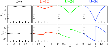
Figure 1: (Color online) Exchange-correlation energies $e_{xc}$ (top) and potentials $v_{xc}$ (bottom) for the homogeneous 3D Hubbard model, as a function of the density, for several values of the interaction $U$.

III.3 Lattice TDDFT

We have seen that DFT can be a viable route to the description of the ground-state properties of strongly correlated systems such as the Hubbard model. A subsequent step would be to look at the dynamical properties of the Hubbard model via TDDFT. Similarly to the case of realistic materials, this could be done at two different levels: 1) One can invoke a linear response treatment to external fields, using the apparatus of many-body perturbation theory, starting from the Kohn-Sham Hamiltonian; 2) In presence of strong time-dependent fields, one could instead resort to a full dynamical description based on TDDFT, by propagating in time the KS equations.

For 1D Hubbard-type Hamiltonians, initial work in the first direction was made in Refs. Arya1 ; Arya2 ; Magyar . In these papers, the main emphasis was on the study of the Hubbard model as a simplified system to gain insight into the general aspects of TDDFT, specifically the kernel $f_{xc}$, and no real-time dynamics was performed. TDDFT in the linear response regime was also applied to a 1D spinless fermion model with nearest-neighbour interactions Schenk08 , where comparisons between exact results and an LDA based on the Bethe-Ansatz were reported. Less is known for $D>1$, and we will present below new results for the linear response of the 3D Hubbard model within the TDDFT-ALDA.

A TDDFT approach to the real-time dynamics of the Hubbard model out of equilibrium was initially considered in Verdozzi08 . In this work, the exact many-body non-equilibrium dynamics of small 1D Hubbard chains of different length and particle density was performed, and from it, via a reverse-engineering procedure, the exact, time-dependent XC potential was obtained, by propagating the time-dependent Kohn-Sham equations:

$$\left(\hat{t}+\hat{v}_{KS}(\tau)\right)\varphi_{\kappa}(\tau)=i\partial_{\tau}\varphi_{\kappa}(\tau).$$ (22)

Eq. (22) is the generalization of Eq. (15) to the time-dependent case. In Verdozzi08 , exact results for the density and the XC potential were compared to those from an approximate $v_{xc}$ obtained within the ALDA, and an analysis of non-local adiabatic effects in $v_{xc}$ was carried out. For the ALDA, in analogy to the static case, the 1D Hubbard model was chosen as the reference systems, so that

$$v^{ALDA}_{xc}(R,t)\equiv v^{BALDA}_{xc}(n_{R}(t)),$$ (23)

where $v^{BALDA}_{xc}(n)$ is given by Eq. (18). In Ref. Verdozzi08 , the treatment was limited to spin-compensated systems, and the spin-dependent case was presented in Polini08 , where TDDFT results were compared to those obtained with the time-dependent DMRG method.

An early rigorous discussion of the formal aspects of TDDFT can be found in Baer08 , where an example of particle density which is non $v_{0}$-representable on the lattice was provided. In Baer08 it was shown that a tight-binding Hamiltonian may in general be unable to reproduce a specific given density. The case considered was that of a dimer with one orbital/site. The issue of $v_{0}$-representability was further analyzed in Ullrich08 ; Verdozzi08 . As shown in Ullrich08 , for a 1D lattice with $L$ sites, the condition $|S_{k}|\leq 2\sqrt{n_{k}n_{k+1}}$, with $S_{k}=\sum_{i=1}^{k}\dot{n}_{i}$ (this expresses current conservation), is necessary and sufficient for $v_{0}$-representability for $N=1$ particle. In a lattice Hamiltonian, the spread of the eigenmodes scales with the hopping term $t$. According to the time-energy uncertainty relation, the range of possible response times scales also with $|t|$. Thus, the larger the hopping, the faster the system can respond in time, and the broader the range of $v_{0}$-representability in time Ullrich08 . The above condition for $S_{k}$ is only a necessary one for $N>1$ Verdozzi08 , also when Hubbard interactions are taken into account. For the special case of a dimer, and using the Cauchy-Schwartz inequality, one can show that the exact density of a Hubbard dimer is $v_{0}$-representable Verdozzi08 .

III.4 Developments in lattice DFT and TDDFT, and applications.

$\bullet$ Electric polarizability.- Very recently, lattice DFT has been used to determine the polarizability $\alpha$ of the 1D Hubbard model AkandeSanvito10 . Results for $\alpha$ from lattice DFT are in good agreement with DMRG ones. In particular, the response of the XC potential is in the same direction of the perturbing potential. Also, the possibility of dealing in lattice DFT with large samples made possible to examine the scaling properties of $\alpha$ AkandeSanvito10 .
$\bullet$ Magnetic properties.- lattice DFT has also been used to study the Hubbard model on the graphene lattice, where it correctly describes the ground-state spin configuration of large graphene clusters (flakes) Harju .
$\bullet$ Quantum Information and Entanglement entropy.- A key quantity to quantum information phenomena is the entanglement, or quantum correlations, of a system. Entanglement has also been studied in the context of quantum phase transitions. A lattice DFT approach to the entanglement entropy of the Hubbard model was presented in FrancaCapelle and, very recently, an explicit density functional for the entanglement was also provided FrancaDamico11 . An TDDFT-ALDA approach to the time evolution of entanglement entropy was used in KarlssonEPL2011 , to discuss the expansion of ultracold fermion clouds in optical lattices.
$\bullet$ Quantum transport.- A combination of DMRG and lattice DFT was used to gain insight into the exact ground-state XC functionals for a correlated-electron model system coupled to external reservoirs SchmittEver08 . The specific model considered was the so-called interacting resonant level model, for which DMRG and DFT conductances were found in good agreement. Very recently, a comparative assessment of lattice DFT and DMRG in transport has been provided in schenk2011 , while an application of the spin-dependent BALDA SDBALDA to quantum transport can be found in Thijssen .

The role of a discontinuity in a time-dependent description of quantum transport has been recently examined within lattice TDDFT-ALDA KSKVG10 . Following the time-evolution of a single Anderson impurity attached to two biased leads, a dynamical notion of the Coulomb blockade was provided. Accordingly, Coulomb blockade manifests itself as a periodic sequence of charging and discharging of the nanostructure. This emerges also from a description based on TDCDFT KurthStefanucci2011 . In passing, we mention that ground-state current DFT has been also applied to lattice models Schenk2 ; AkandeSanvito11 . For 1D Hubbard rings threaded by a magnetic flux, the effects of lattice impurities on the persistent currents and on the Drude weights has also been examined AkandeSanvito11 .
$\bullet$ Connection to many-body approximations, and critical analysis of the local density approximations.- The so-called variational approach to TDDFT ABL ; varfxc has the advantage of a systematic inclusion of many-body contributions in the XC potential. In this way non-locality in space and memory effects can be properly included, once $v_{xc}$ is retrieved from the many-body self-energy via the time-dependent Sham-Schlüter equation RobertShamSh96 . This well established relation between many-body perturbation theory and TDDFT on the Keldysh contour was numerically examined in pva2 , by looking at exchange-correlation potentials obtained via time-dependent reverse engineering using the time-dependent densities from the KBE. The performance of two self-interaction correction schemes for the 1D Hubbard model has been scrutinized in CapelleSIC , while a shortcoming of the BALDA was pointed out in Capelle2kf4kf , specifically its capability to reproduce correctly the Friedel oscillations in the inhomogeneous 1D Hubbard model. Finally, the lattice DFT for the 1D Hubbard model has been used to illustrate the Hohenberg-Kohn mapping between densities and ground-state wave functions in terms of the metric-space aspects of the Hilbert space Capelle_Metric .
$\bullet$ Cold atoms and dynamical quenches.- In optical lattices opticalattices , it is possible to study fermionic and bosonic atoms with repulsive and/or attractive interactions and (because an accurate tunability of the lattice parameters is possible) often more directly and easily than in solid-state experiments. Trapped ultracold atoms on an optical lattice permit to study different ground-state scenarios for the Hubbard model. Lattice DFT and lattice TDDFT have been used to investigate these systems. For example, an extensive study of the ground-state properties of trapped repulsive fermions in a 1D Hubbard lattice was provided in XianlongPoliniTosiCampoCapelleRigol06 . Here, a comparison of lattice DFT and quantum Monte Carlo density profiles was performed, and an detailed microscopic picture of the consequences of the interplay between particle-particle interactions and confinement was given.

A similar analysis within lattice DFT has been carried out in Hu2010 for the case of a 1D Hubbard model with attractive interactions. For lattice TDDFT, a first application to fermions on optical lattices was to compare (spin-dependent) ALDA and DMRG dynamics after the quench of a localized external perturbation Polini08 . A more recent study of the dynamics after a local quench can be found in Xianlong2010 . The effect of a global quench in 1D, i.e. the removal of a parabolic trapping potential, was studied in KarlssonEPL2011 , where quenches of different speed (from adiabatic to sudden) were applied, showing a dynamical self-stabilization of the Mott insulator phase in the density profile. In this work, the role of entanglement as a pointer of dynamical phase changes was also analyzed, and the system’s thermalization was discussed from a TDDFT perspective. Finally, the beating and damping regimes of the Bloch oscillations in a 3D Hubbard optical lattice has also been investigated with TDDFT DKAPCV11 .

III.5 TD[C]DFT on the lattice: Runge-Gross theorem and connections to lattice TDDFT

There is at present no formulation of the Runge-Gross (RG) theorem of TDDFT for the lattice. The reason for this has been explicitly discussed in KurthStefanucci2011 and, in essence, it has to do with the fact that a reductio ad absurdum strategy, along the lines of the RG theorem, is not possible. This is because, in the proof for the lattice, terms related to the one-particle density matrix appear, which do not carry a definite sign. This observation corroborates the fact that, for lattice Hamiltonians, one can actually find examples which contradict the uniqueness of the correspondence between densities and potentials.

If one adopts the bond current as the basic variable, a one-to-one mapping can be established GSEPMC10 betweeen current densities and Peierls phases Peierls ; Graf of the bond-hopping terms. In this way a rigorous formulation of TDCDFT on the lattice becomes possible GSEPMC10 ; Tokatly11 ; KurthStefanucci2011 , either in analogy with the original RG theorem GSEPMC10 , or via a reformulation based on non-linear differential equations methods Tokatly11 .

In addition to establish a rigorous connection also for the densities, a lattice TDCDFT formulation has the further advantage of being valid in the presence of magnetic fields of a general kind, which enter via the Peierls phases (more precisely, the Peierls phases describe the effect of the vector potential $\bf{A}$). This is not the case of TDDFT; it can be easily shown that, by a local gauge transformation, the scalar onsite potentials of TDDFT can be removed from the Hamiltonian while, at the same time, introducing Peierls phases $\phi_{ij}=\alpha_{i}-\alpha_{j}$ in the hopping term between sites $i$ and $j$. The sum of phases of such specific form over a lattice plaquette adds up to zero, and corresponds to a null line integral of ${\bf A}$ over a closed loop, i.e. to a zero magnetic flux across the plaquette. For these cases, i.e. in the absence of magnetic fields, TDDFT could be used; otherwise, TDCDFT should be considered.

In conclusion, care must certainly be exerted in using lattice TDDFT when dealing with issues for which the uniqueness of the density-potential mapping is relevant. It should, however, still be possible to use lattice TDDFT on heuristic grounds, even if, at present, the practical implications of the lack of a rigorous formulation largely remain to be seen.

IV Kadanoff-Baym Dynamics

The main aim of the non-equilibrium Green’s function (NEG) technique KB-book ; Keldysh ; Danielewicz ; Bonitzbook is to obtain expectation values of single-particle operators and the total energy of an interacting system subject to an external field. The NEG technique is used in a wide variety of fields, treating both real and model systems Jauho ; Stefanucci04 ; Robert ; Bonitzdots ; Galperin ; Thygesen1 ; Olevano ; RobertHubb ; Freericks ; pva1 . The method has the advantage of having a direct connection to MBPT, in which conserving KB-book approximations of increasing complexity can be constructed systematically and where memory effects Danielewicz ; Bonitzbook are automatically built in. However, when the NEG technique is used in conjunction with MBPT, the method has also a few limitations, some of which are practical in character. Before discussing further this point, we proceed now to a brief summary of the approach.

IV.1 Formalism

The central object in the NEG echnique is the path-ordered, one-particle Green’s function,

$$G(1,2)=-i\langle T_{\gamma}\left[\psi(1)\psi^{\dagger}(2)\right]\rangle,$$ (24)

where, in more detail, 1 denote single-particle space/spin and time labels, $r_{1}\sigma_{1}t_{1}$. Here, $T_{\gamma}$ orders the times $t_{1},t_{2}$ on the Keldysh contour Keldysh $\gamma$ ($t_{1},t_{2}$ can be either real or imaginary), and the field operators are in the Heisenberg picture; the brackets $\langle\rangle$ denote averaging over the initial state (ground state or thermal equilibrium).

The $G$ is determined by the Kadanoff-Baym equations, its equations of motion. Specializing to time $t_{1}$, we have notation

$$\left(i\partial_{t_{1}}-h\left(t_{1}\right)\right)G\left(t_{1},t_{2}\right)=\delta(12)+\int_{\gamma}\Sigma\left(t_{1},t\right)G\left(t,t_{2}\right)dt.$$ (25)

Here $h$ is the single-particle Hamiltonian and $\Sigma$, the kernel of the integral equation, is the self-energy, treated within a given many-body approximation (MBA). Eq. (25) and the one corresponding to $t_{2}$ are solved numerically, and for non-isolated systems, $\Sigma$ contains an additional contribution, the embedding self-energy $\Sigma_{emb}$, to treat the coupling system-environment Stefanucci04 ; RobertHubb ; pva2 .

The MBA:s we consider in this paper are the second Born, the $GW$ and the $T$-matrix approximations (BA, GWA and TMA respectively). The self-energy in the BA includes all terms up to second order. The GWA Hedin amounts to add up all the bubble diagrams which give rise to the screened interaction, $W=U+UPW$, where $P(12)=G(12)G(21)$. In this case the self-energy is $\Sigma(12)=G(12)W(12)$. In a spin-dependent treatment of the TMA TMA ; pva2 one constructs the $T$ by adding up all the ladder diagrams, $T=\Phi-\Phi UT$, where $\Phi(12)=G(12)G(12)$. The expression of the self-energy then becomes $\Sigma(12)=\int U(13)G(43)T(34)U(42)d34$ (for further details see e.g. pva2 ).

All these approximations are conserving KB-book , i.e. the macroscopic conservation laws (for the energy, the number of particles, etc.) hold, which is a key requirement for time dynamics. The fact that the approximations are conserving does, however, not guarantee the soundness of other important features, as shown in the next Section.

IV.2 Some drawbacks of KBE+MBPT

On the practical side, a first limitation is that the Green’s function is a two-point function and thus scales quadratically with the propagation time. A second one is that the KBE must be solved self-consistently with a non-local kernel at every point in time. Currently, this is viable for very small systems, whilst larger ones can only be treated in the steady state regime (where only one time variable is required).

On the more fundamental side, the NEG approach within MBPT manifests other undesirable traits, for example perturbation schemes may break down for strong interactions. However, even for converging schemes, unphysical features can emerge, which can sometimes play an important role. For example, in MBPT, the ground-state spectral function of a finite system contains infinitely many poles, whereas in the exact solution the number of poles in finite. Moreover, in the KBE-based time dynamics, the MBA:s introduce an artificial correlation induced damping which, in some cases, can completely dominate the evolution. For finite systems, such damped dynamics results in a steady (i.e. never decaying) state. In extended systems, a similar behavior is observed, but with a difference, namely arbitrarily long-lived states occur which, however, eventually decay into a unique steady state. This behavior is certainly artificial in finite systems, while its physical soundness in extended systems is much harder to establish.

Another drawback concerns KBE and correlation functions: It is well known that single-particle Green’s functions give access to certain two-particle properties such as, e.g., the total energy. In particular, they can be used to determine the density-density correlation function at equal times, e.g. the so-called double occupancy, $\left<\hat{n}_{R\uparrow}\hat{n}_{R\downarrow}\right>$ pva_cond ; gooding . However, within conserving MBA:s, correlation functions may violate important properties such as positiveness pva_cond .

In spite of these possible drawbacks, the KBE, together with a MBPT approach to the self-energy, offer the great advantage of incorporating non-locality and memory effects on equal footing. For this reason they will be used in the next Section to benchmark our TDDFT results.

V Scrutinizing the linear response formalism and the ALDA in lattice models

This section presents original results for three different topics. The first one is an illustration, by means of a simple model system, of the problems one may encounter when using the LSS within the linear response formalism of TDDFT.

We then present two applications of lattice TDDFT, which offer a clear illustration of the limitations (but also of the positive aspects) of the ALDA. In the first case, we study the density response function for the 3D Hubbard model, and we use an $f_{xc}^{ALDA}$ obtained from DMFT (Sect. III.2). The functional form of the kernel $f_{xc}^{ALDA}$ is also discussed. In the second example, we study the non-linear, TDDFT-ALDA response of a finite cluster to strong, time-dependent perturbations. The $v_{xc}$ used in the ALDA is also in this case obtained from DMFT. The TDDFT results will be compared to exact ones, and to those from the Kadanoff-Baym dynamics introduced in Sec. IV.

V.1 Inversion of the non-interacting response

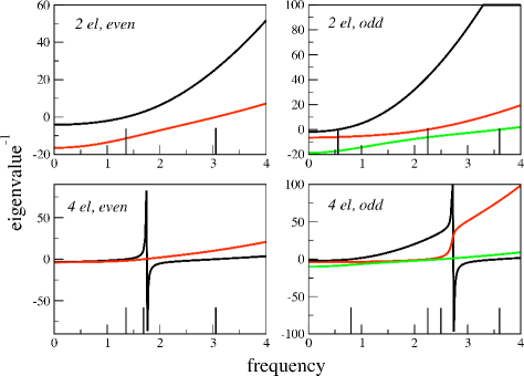
Figure 2: (Color online) Inverse of the eigenvalues of $\chi_{0}$, for a six-site, spin-compensated chain with 2 and 4 electrons, as function of the frequency. The longer vertical ticks on the frequency axis denote the excitation energies (see main text).

It was long hoped that the exact-exchange approximation within TDDFT would provide a reasonable XC kernel which is both non-local and energy dependent and thus constituting a significant step beyond the usual adiabatic approximations. As mentioned in Sect. II, these hopes have recently evaporated, the main reason being zeros in the non-interacting response function. This problem has actually been pointed some time ago MK . In the spirit of the model investigations at the heart of the present work we will here demonstrate the problem in some model cases.

The non-interacting response function $\chi_{0}$ can always be written as

$$\chi_{0}({\bf r},{\bf r}^{\prime};\omega)=\sum_{q}\frac{2\omega_{q}f_{q}({\bf r})f_{q}^{*}({\bf r}^{\prime})}{\omega^{2}-\omega_{q}^{2}}$$ (26)

where the index $q$ is a double index $q=(k,k^{\prime})$ and $\omega_{q}=\epsilon_{k^{\prime}}-\epsilon_{k}$ is an excitation energy given by the energy difference between an unoccupied ($\epsilon_{k^{\prime}}$) and an occupied ($\epsilon_{k}$) eigenvalue of the basic one-electron Hamiltonian. The functions $f_{q}$ are excitation functions consisting of the corresponding products between an unoccupied, $\varphi_{k^{\prime}}^{*}({\bf r})$, and occupied, $\varphi_{k}({\bf r})$, orbital of the same Hamiltonian. Due to the orthogonality of the orbitals $\{\varphi_{k}\}$, the functions $f_{q}$ always integrate to zero, resulting in the well known property of $\chi_{0}$ of a finite system

$$\int\chi_{0}({\bf r},{\bf r}^{\prime})\;d^{3}r^{\prime}=0.$$ (27)

This means that the response function $\chi_{0}$ always has a zero eigenvalue at all frequencies, which is a reflection of the physical fact that there can be no charge response to a constant potential. Unfortunately, the response $\chi_{0}$ also has other zero eigenvalues at specific frequencies. If we first consider a two-electron problem, the lowest orbital $\varphi_{0}$ is doubly occupied and all other orbitals are unoccupied. The complete set of orbitals $\varphi_{k}$ are, of course, linearly independent, a fact which is not altered by removing the lowest member $\varphi_{0}$ from the set. Neither is this fact altered by multiplying all the remaining orbitals in the set by the same function $\varphi_{0}$. Consequently, in this case, all the excitation functions are linearly independent. Assuming for a moment that $\chi_{0}$ has an eigenvector $u({\bf r})$ with a vanishing eigenvalue we find that

$$\sum_{q}\frac{2\omega_{q}f_{q}({\bf r})u_{q}}{\omega^{2}-\omega_{q}^{2}}=0,$$ (28)

where the coefficients $u_{q}$ are the projections of the eigenfunction $u$ onto the excitation functions $f_{q}$. But, since the excitation functions are linearly independent, all coefficients in this linear combination of the $f_{q}$:s must vanish and, since the frequency dependent factors are non-zero, we are led to the conclusion that all the coefficients $u_{q}$ must vanish. But, again, the only function $u$ which is orthogonal to all the excitation functions $f_{q}$ is a constant and we have recovered the already known case. Thus, in the two-electron case, there can be no additional zero eigenvalues of $\chi_{0}$.

Proceeding now to more than two electrons, we have several sets of excitation functions, one for each occupied orbital. Although all functions within a particular set are linearly independent among themselves, we find it highly unlikely that the conjunction of all sets are linearly independent. Indeed, every set is almost a complete set by itself. One would therefore expect to be able to expand a member of one set in the combined functions of two other sets. Consequently, by varying the frequency and the coefficients $u_{q}$ in the vanishing sum above, Eq.(28), one would expect to be able to arrive at a particular vanishing linear combination of the excitation functions $f_{q}$. In the spirit of the present paper, we will illustrate these points on a simple non-interacting linear chain of atoms with one orbital per site, no one-site energies, and only nearest neighbour hopping- the same for each spin channel.

Choosing four atoms in the chain and two electrons with opposite spin, the relevant Hamiltonian is 4x4 and we have only three excitation functions with corresponding excitation energies - from the ground state to each of the three unoccupied states. As it turns out and is easily verified on the back of an envelope, the three excitation functions in a four-dimensional space are definitely linearly independent and there are thus no additional zero eigenvalues of $\chi_{0}$.

Turning then to four electrons, two for each spin channel, we obtain four excitation functions from each of the two occupied states to each of the remaining two unoccupied states. As easily verified, two excitation functions are identical and so are their corresponding excitation energies. In the sum above, Eq.(28, these two functions will contribute equally and both are included by multiplying one of the terms by two. Any linear chain has, of course, mirror symmetry around the mid point, a fact which substantially reduces the necessary algebra - especially for the few-site cases. The response function $\chi_{0}$ splits into a sum of an even and an odd contribution and so do all the excitation functions. In the present case, the two even excitation functions are identical and, consequently, the even part of $\chi$ consits of only one term which cannot be orthogonal to anything but the constant vector. The two odd excitation functions are easily seen to be linearly independent by inspection. Thus, also in the four-electron case, there are no extra zero eigenvalues of $\chi_{0}$ as long as there are four sites.

Including six sites in the model, we immediately approach the above discussed general behaviour of $\chi_{0}$. Looking first at the two-electron case, we obtain five excitation functions and energies. The calculations now become a little too complicated to carry out by hand but are still rather trivial. The six-by-six determinant of the five excitation functions plus the constant vector turns out to be non-singular, thus demonstrating all excitation functions to be linearly independent. Hence, there are no additional vanishing eigenvalues of $\chi_{0}$, in keeping with the general discussion above.

Having instead four electrons on the six sites gives us eight excitation functions of which two turn out to be identical. But there is no way the remaining seven can be linearly independent in a six-dimensional space. As discussed above, we would then expect that a particular choice of frequency could result in coefficients giving rise to a vanishing linear combination of excitation functions and thus a zero eigenvalue of $\chi_{0}$. In Fig. 2 we have plotted the inverse of the five non-trivial frequency dependent eigenvalues of $\chi_{0}$ for the even and the odd channels - for both the two-electron case and the four-electron case. We see that these inverse eigenvalues are all nice smooth functions of the frequency in the former case. We also see that two eigenvalues in the four-electron case pass zero at particular frequencies away from the excitation energies - one in the odd channel and one in the even channel. These results corroborate the correctness of the general discussion above.

V.2 Linear response in the ALDA for the 3D Hubbard model.

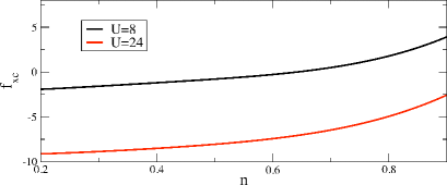
Figure 3: (Color online) The ALDA exchange-correlation kernel $f^{ALDA}_{xc}$ for $U=8$ and $U=24$ obtained by differentiating $v_{xc}$ with respect to the density.

In analogy to the continuum case, the general expression for the XC kernel $f_{xc}$ on the lattice is

$$f_{xc}({\bf R},{\bf R^{\prime}};t,t^{\prime})=\frac{\delta v_{xc}({\bf R},t)}{\delta n_{\bf R^{\prime}}(t^{\prime})}.$$ (29)

In the ALDA, an ordinary derivative in the density is performed, and the space and time dependence is entirely local:

$$f_{xc}^{ALDA}({\bf R},{\bf R^{\prime}};t,t^{\prime}) =\frac{dv_{xc}(n_{\bf R}(t))}{dn_{\bf R^{\prime}}(t^{\prime})}$$

$$=v^{\prime}_{xc}(n_{\bf R}(t))\delta_{\bf RR^{\prime}}\delta(t-t^{\prime}),$$ (30)

and $f_{xc}\equiv f_{xc}^{ALDA}({\bf q},\omega)$, i.e. $f_{xc}$ only depends of the (uniform) ground-state density of the system. In the Hubbard model of Eq. (8), the bare interaction $U$ is also local in time and space. Accordingly, for the 3D homogeneous Hubbard model, and in the (${\bf q},\omega$) space, the ALDA density-density response function $\chi(\textbf{q},\omega)$ is

$$\chi(\textbf{q},\omega)=\frac{\chi_{0}(\textbf{q},\omega)}{1-(U+f_{xc})\chi_{0}(\textbf{q},\omega)}$$ (31)

Here, $\chi(\textbf{q},\omega)$ is the Fourier transform of the retarded response function

$$\chi({\bf R},t)=-i\theta(t)\langle\left[\tilde{n}_{\bf R}(t),\tilde{n}_{\bf 0}(0)\right]\rangle_{gs},$$ (32)

and $\tilde{n}_{\bf R}(t)=\hat{n}_{\bf R}(t)-\langle\hat{n}_{\bf R}(t)\rangle$, with $\hat{n}_{\bf R}(t)=\hat{n}_{\bf R\uparrow}(t)+\hat{n}_{\bf R\downarrow}(t)$. Furthermore, $\chi_{0}$ is the response function of the Kohn-Sham system,

$$\chi_{0}(\textbf{q},\omega)=\frac{2}{(2\pi)^{3}}\int d^{3}k\frac{n_{F}(\epsilon_{\textbf{k}})-n_{F}(\epsilon_{\textbf{k}+\textbf{q}})}{\epsilon_{\textbf{k}}-\epsilon_{\textbf{k}+\textbf{q}}+\omega+i\eta},$$ (33)

where $\epsilon_{\bf k}=-2t(\cos k_{x}+\cos k_{y}+\cos k_{z})$ is the single particle energy dispersion in the 3D simple cubic lattice, $n_{F}(\epsilon)$ is the Fermi function (we work at zero temperature) and the integral in ${\bf k}$ is performed over the first Brillouin zone.

Before presenting the random-phase-approximation (RPA) and TDDFT-ALDA results for $\chi$, it is useful to discuss briefly the features of $f_{xc}$ in the ALDA. In Fig. 3, we show $f^{ALDA}_{xc}$ as a function of the density $n$. Since $f_{xc}^{ALDA}(n)=f_{xc}^{ALDA}(2-n)$, we can consider results for $n\leq 1$. Furthermore, the results $f_{xc}$ for $n\leq 0.2$ and $n\geq 0.95$ exhibit significant noise, and thus are not displayed. In Fig. 3, we see clearly one of the interesting features of $f_{xc}^{ALDA}$, namely the XC kernel can be either negative or positive also1D . This is especially evident for $U=8$, and can also immediately be gathered from the results for $v_{xc}$ in Fig. 1. Thus we see that, depending on the band filling, $f_{xc}^{ALDA}$ can reduce or reinforce the effect of the bare interaction $U$ in Eq. (31). This is at variance with the usual case, where the XC kernel tend always to induce an effective interaction which is reduced with respect to the bare one. The other important aspect in the XC kernel is its behavior at $n=1$. Looking again at Fig. 1, we note that the discontinuity in $v^{DMFT}_{xc}$ for $U>U^{Mott}_{c}$ (in our case $U=24$) will introduce a (Dirac’s delta-like) spike in the XC kernel at $n=1$. This singular behavior would be absent for $U<U^{Mott}_{c}$ in 3D, but always present in 1D where $v_{xc}$ is discontinuous for any value of $U$.

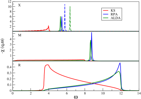
Figure 4: (Color online) The imaginary part of $-\chi(\textbf{q},\omega)$ for $U=8$, as a function of $\omega$, at three high symmetry points in the Brillouin zone. The chosen ${\bf q}$ values are $X=(\pi,0,0)$, $M=(\pi,\pi,0)$ and $R=(\pi,\pi,\pi)$ (note the different vertical scale for the three panels). The average density is $n=0.5$, i.e. quarter filling. In each panel, the solid curves refer to the Kohn-Sham, RPA and ALDA cases (red, blue and green, respectively). The effect of $f_{xc}$ for this filling is to give a reduced effective interaction, with the ALDA peak shifted to the left of the RPA one. For the point $X$ we also show results for another filling ($n=0.85$, dashed curves), where $f_{xc}$ is positive. In this case, the ALDA peak (green curve) is at the highest energy.

Results for $\chi({\bf q},\omega)$ for three values of ${\bf q}$ are shown in the three panels of Fig. 4. The systems density that we consider is quarter filling, i.e. $n=0.5$, and $U=8$. In each panel, there are three solid curves which represent the imaginary part of the Kohn-Sham (red curve), RPA (blue curve) and TDDFT-ALDA versions of $-\chi({\bf q},\omega)$ (the dashed curves in the top panel will be discussed momentarily). For the RPA and ALDA curves, we see sharp structures, outside the $\chi_{0}$ continuum region, corresponding to the zeros of $1-(U+f_{xc})\chi_{0}(\textbf{q},\omega)$. Such peaks describe the plasmonic features of our system. We mention in passing that we have performed several test of our numerics, including a (successful) verification the of the f-sum rule,

$$M(\textbf{q})=-\frac{2}{\pi}\int\text{Im}(\chi_{0}(\textbf{q},\omega))\omega d\omega=$$

$$-\frac{2}{(2\pi)^{3}}\int d^{3}k\langle c^{\dagger}_{k}c_{k}\rangle(\epsilon(\textbf{k}+\textbf{q})+\epsilon(\textbf{k}-\textbf{q})-2\epsilon(\textbf{k})).$$ (34)

It interesting to note that, for the solid curves, the RPA peaks are always at higher energy than the ALDA ones. This is easily explained considering that at quarter filling, and for $U=8$, $f^{ALDA}_{xc}$ is negative (Fig. 3), thus screening the bare $U$. However, it also clear that for densities close to half-filling, say $n=0.85$, the XC kernel at $U=8$ is positive, giving ALDA peaks at energies higher than the RPA ones. This situation is shown in the top panel of Fig. 4, for one value of $\bf q$, and it corresponds to the dashed curves in that panel.

A similar behavior can be observed in real space. In Fig. 5, which refers to the case of quarter filling and $U=8$, the four panels show the dependence of $\text{Im}\chi({\bf R},\omega)$ on the distance $|{\bf R}|$ along the $x$-axis (as one goes away from $R=0$, the response function diminishes quite rapidly). The principal effect of the correlations is to move the structures in $\text{Im}\chi$ to higher energies with respect of the Kohn-Sham results. Furthermore, we can notice how the ALDA profiles are always shifted at lower energies with respect to those of the RPA, due to the negative value of $f_{xc}^{ALDA}$ when $n=0.5$ and $U=8$.

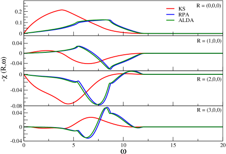
Figure 5: (Color online) The linear response $\chi(\textbf{R},\omega)$ as a function of $\omega$ for $U=8$, for different values of R.

In general, the pair correlation function (and thus the density response function) is a careful indicator of the accuracy of a many-body approximation. Thus, looking at properties which involve $\chi$ can provide a severe test to assess the performance of the ALDA. For example, the density-density response function can be used to compute the ground-state energy of the system. More specifically, via the connection to the dynamical structure factor $S(\bf{q},\omega)$, one can determine the local double occupancy $d_{\bf R}=\langle\hat{n}_{\bf R\uparrow}\hat{n}_{{\bf R}\downarrow}\rangle$. We have used $\chi$ in the RPA and the ALDA to compute $d_{\bf R}$, and the results are reported in Table 1. Two general features can be noted. The first is that in some cases the RPA and ALDA results for $d_{\bf R}$ are negative. Since $d_{\bf R}$ is manifestly positive, this is an adverse outcome of the ALDA, and is rather general in character. Indeed, it is a long established fact that, in the RPA Lindhard , pair correlations for the electron gas at metallic densities are strongly negative at short distances Alf ; more recently, the same problem has been also experienced within the self-consistent GWA and BA Holm ; Dimercondmat .

The second general trait in Table 1 is related to the sign of $f_{xc}$: at quarter filling, where the $f_{xc}$ is negative, we get an effective lower interaction, which tends to increase the ALDA double occupancy with respect to the one from the RPA. On the other hand, at $n=0.85$, the $f_{xc}$ for $U=8$ is positive, and thus instead increases the interaction, which results in a lower double occupancy.

As a conclusive remark, while our results for the double occupancy point out a shortcoming of the ALDA, they also indicate that the problem with the sign of $d_{\bf R}$ could be less acute than in the continuum case. In fact, at least for the cases we considered, double occupancies in the ALDA are only slightly negative and, most likely, this is a consequence of the natural cut-off introduced by the lattice at short distances.

Parameters	$d_{DMFT}$	$d_{KS}$	$d_{RPA}$	$d_{ALDA}$
$U=8,n=0.5$	0.036	0.062	−0.010	−0.007
$U=24,n=0.5$	0.016	0.062	−0.047	−0.035
$U=8,n=0.85$	0.114	0.178	+0.072	+0.059

Table 1: Double occupancies $d=\langle n_{\uparrow}n_{\downarrow}\rangle$ obtained from DMFT, compared against results from linear response. Results from $\chi_{0}$, $\chi_{RPA}$ and from $\chi_{ALDA}$ are shown.

V.3 Exact, ALDA and Kadanoff-Baym real-time dynamics in a small cluster.

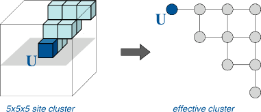
Figure 6: (Color online). Original 125-site cluster (left) and its effective image (right). In the original cluster, all sites are related by symmetry to the 10 sites explicitly shown. Accordingly, the site $0$ is the same in the two clusters.

The system we choose to compare TDDFT-ALDA, exact, and Kadanoff-Baym results is a simple cubic cluster with $5^{3}$ sites and open boundary conditions (Fig. 6, left). We choose the cluster to be highly inhomogeneous, by having a single interacting impurity in the center $R=0$, e.g., $U_{R}=U\delta_{R0}$ in Eq. (8). We also set $w_{R}(\tau)=w_{0}(\tau)\delta_{R0}$. Due to cubic symmetry, only $N_{sym}=10$ out of $125$ one-particle eigenstates, those with non-zero amplitude at $R=0$, determine the static and time-dependent density at $R=0$, making the size of the exact configuration space manageable MCCV87 , in the guise of an effective 10-site cluster (Fig. 6, right). Furthermore, if $\epsilon_{R\neq 0}=0$, further use of symmetry gives $N_{sym}=7$. In this case, the shape of the cluster corresponds to the $R=0$ impurity directly connected with to all the other 6 sites. However the $R\neq 0$ states are not connected directly to each other, but only to the impurity. In the ground state, the way $N_{e}$ electrons in the cluster distribute between the $N_{sym}$ active and $125-N_{sym}$ spectator states corresponds to the exact many-body eigenstate with lowest energy. As a overall remark, we note that the simplification due to symmetry is very peculiar to our choice of a local interaction at a single site, and permits us to obtain exact dynamical results in 3D for a quite large cluster. Furthermore, such simplification remains in the presence of a time-dependent perturbation localized at the impurity site.

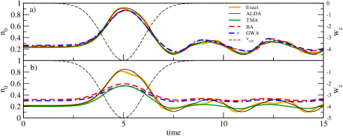
Figure 7: (Color online) Time-dependent density, $n_{0}(\tau)$, of the central (interacting) site in a 5x5x5 simple cubic cluster subject to a Gaussian potential $W_{g}(\tau)=-5e^{-\frac{\left(\tau-5\right)^{2}}{2}}$ (thin black dashed). The curves correspond to exact (thick solid orange), ALDA (thin solid black), BA (red dashed), GWA (blue dot-dashed) and TMA (solid green). The number of particles per spin of the equivalent cluster is 2. In a) $U=8$ and in b) $U=24$.

In Fig. 7 we study the time-dependent density of the interacting impurity when subject to a slowly varying pulse for different values of the interaction strength. This is a situation in which the ALDA is expected to be appropriate. In the ground state, before the perturbation has been introduced, the systems are in the low density regime. The reason of this choice is that of the three MBA:s we consider, one of them, the TMA, performs rather well at these densities pva1 , while the BA and GWA are not good in any of the regimes we considered.

In Fig. 7, where the interaction strength is weak and the external field is slowly varying, we see that the ALDA, as well as the KBE+MBPT, give an overall good description, both in the time window where the perturbation is actually present, and afterwards, when the system is performing free oscillations. When the interaction strength is geared up in Fig. 7b we clearly see that the ALDA is superior to all the KBE results from the MBA:s, while the TMA performs better than the BA and the GWA. It is fair to say that overall ALDA provides a good description for these slow external fields.

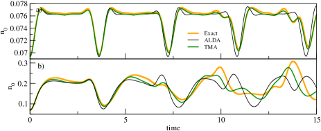
Figure 8: (Color online) Time-dependent density, $n_{0}(\tau)$, of the central (interacting) site in a 5x5x5 simple cubic cluster subject to a step potential, $W_{g}(\tau)=W_{0}\Theta(\tau)$. The curves correspond to exact (thick orange), ALDA (thin black) and TMA (green). The number of particles per spin of the equivalent cluster is 1. In a) $W_{0}=-0.2$ and in b) $W_{0}=-2$.

In Fig. 8, we show the exact, ALDA, and TMA results for case of a moderate interaction strength and a step perturbation (BA and GWA, not presented, perform quite poorly). In this case, the shortcomings of the ALDA are evident. For example, the ALDA does not reproduce the long-time oscillations properly: in Fig. 8a, the ALDA performs well for $\tau\lesssim 4$, but after that, ALDA suffers an increasing dephasing with respect to the exact and TMA solutions. On the other hand, the TMA and the exact curve are in very good mutual agreement for this situation, (see e.g. the region $\tau\approx 14$), which corresponds to a highly non-adiabatic, but weak, perturbation.

For a stronger step perturbation (Fig. 8b), the KBE+MBPT approach, represented here by the TMA, is able to describe the history dependence quite well, and significantly better than the ALDA, which becomes unreliable. However, when both the interaction is strong and the external field is highly non-adiabatic, both the ALDA and the KBE+MBPT fail to describe the transient dynamics (not shown).

To summarize, the ALDA, in suitable conditions, i.e. for slow perturbations, can perform well. However, we wish to remark that the ALDA we have considered here accounts for the effect of correlations in a non perturbative way, since it is obtained from DMFT reference calculations. Otherwise, for systems with much stronger interactions, a failure of ALDA should be expected also for external fields which vary slowly in time.

VI Conclusions

The application of time-dependent density-functional theories to the non-equilibrium dynamics of lattice models has recently received some attention in the scientific community. Conceptually firm ground has now been established for approaches which use the current density (or, more properly, the lattice bond current) as basic variable. By contrast, the early TDDFT-like approaches for lattice systems made use of the density as the basic variable. On the lattice, a density-based approach lacks a completely rigorous formulation, but it appears possible to consider it on heuristic grounds, in the sense that the missing rigor should not be of significant practical consequence.

It is in this spirit that in this work we have adopted lattice TDDFT as an investigative tool to discuss two general aspects of TDDFT, which are present also in the continuum formulation. These are the linear response formalism in TDDFT, and the adiabatic local density approximations (ALDA).

Instrumental to this strategy, the first part of our paper has been devoted to short reviews of linear response theory, lattice TDDFT, and also of the non-equilibrium Green’s function method: the latter method was used to benchmark the results from lattice TDDFT.

In the second part of this contribution, where our new results are presented, we have studied the linear and non-linear response of 1D and 3D lattice Hubbard-type models. We find that the limitations encountered in the continuum case by the TDDFT linear response persist in simple 1D lattice model systems. Furthermore, an ALDA treatment for the linear response of the 3D homogenous Hubbard model exhibits an important pitfall which is also present in the continuum case, namely short-range correlations are incorrectly accounted for by the ALDA, albeit at a lesser extent than for the electron gas.

We have also shown that the sign of the ALDA XC kernel can change depending on the values of $U$ and the density, and that for large enough values of $U$, $f_{xc}$ can exhibit a singular behavior at half-filling (due to the discontinuity in $v_{xc}$, which in turn is indicative of the Mott-Hubbard metal-insulator transition). Such characteristics of $f_{xc}$ are clearly visible in the energy dependence of the density response function. To our knowledge, the qualitative features of $f^{ALDA}_{xc}$ just mentioned have no correspondence in the available XC kernels for continuum case. On general grounds, we expect they should be robust against the inclusion of non-local, non-adiabatic effects.

There have been attempts to go beyond the ALDA and simultaneously include non-locality and frequency dependence in the kernel $f_{xc}$. Several of these attempts have originated in the LSS or, equivalently, in the variational approach starting from the Klein functional, and have, therefore, led to severe difficulties as discussed in the introduction. The problem is associated with use of the LSS or, within the variational appoach, with starting from the Klein functional. The ”perpetrator” is the double inversion of the $\chi_{0}$ within these formulations. We can already anticipate that this particular problem will not be present if one instead choses to start from the more sophisticated Luttinger and Ward (LW) functional LW . Whether or not the LW functional will give rise to other problems remains to be seen. Work along these lines is underway.

In the non-linear case, our results can be summarized as follows. An ALDA which accounts for the effect of correlations in a non-perturbative way, can provide a satisfactory description of the non-equilibrium dynamics induced by slow perturbations. When non-local and non-adiabatic effects play an important role, i.e. for fast perturbations, the ALDA is clearly insufficient. This is especially evident if one compares the exact, TDDFT-ALDA and Kadanoff-Baym dynamics. In the latter, effects beyond the ALDA are present, and are seen to be necessary to get a good agreement with the exact data.

In conclusion, both in the linear and non linear cases, our results for lattice models confirm that going beyond the ALDA is certainly necessary in many instances, and that lattice models can be a useful way to scrutinize fundamental open issues in TDDFT and to explore possible avenues for improvement.

References

- (1) Time-Dependent Density-Functional Theory, edited by M.A.L. Marques, C. A. Ullrich, F. Nogueira, A. Rubio, K. Burke, E.K.U. Gross (Springer Verlag, 2006)
- (2) P. Hohenberg and W. Kohn, Phys. Rev. 136, B 864 (1964).
- (3) W. Kohn and L.J. Sham, Phys. Rev. 140, A 1133 (1965).
- (4) E. Runge and E. K. U. Gross, Phys. Rev. Lett. 52, 997 (1984).
- (5) R. van Leeuwen, Phys. Rev. Lett. 82, 3863 (1999).
- (6) M. Ruggenthaler and R. van Leeuwen, arXiv:1011.3375.
- (7) N. T. Maitra, T. N. Todorov, C. Woodward, K. Burke, Phys. Rev. A. 81, 042525 (2010).
- (8) T. C. Li and P. Q. Tong, Phys. Rev. A 31, 1950 (1985).
- (9) T. C. Li and P. Q. Tong, Phys. Rev. A 34, 529 (1986).
- (10) M. Di Ventra and R. D’Agosta, Phys. Rev. Lett. 98, 226403 (2007).
- (11) O. -J. Wacker, R. Kümmel and E. K. U. Gross, Phys. Rev. Lett. 73 2915 (1994).
- (12) A.K. Rajagopal and F. A. Buot, Phys. Rev. B 52, 6769 (1995).
- (13) S. K. Ghosh and A. K. Dhara, Phys. Rev. A 38, 1149 (1988).
- (14) G. Vignale, Phys. Rev. B 70, 201102(R), (2004).
- (15) G. Stefanucci, E. Perfetto, and M. Cini, Phys. Rev. B 81, 115446 (2010).
- (16) I. Tokatly, Phys. Rev. B 83, 035127 (2011).
- (17) S. Kurth and G. Stefanucci, arXiv:1012.4296, to be published in Chemical Physics.
- (18) R. van Leeuwen R, Phys. Rev. Lett. 80, 1280 (1998).
- (19) R. van Leeuwen, N. E. Dahlen, G. Stefanucci, C.-O. Almbladh, and U. von Barth, Lect. Notes Phys. 706, 33 (2006).
- (20) A. Zangwill and P. Soven, Phys. Rev. A 21, 1561 (1980).
- (21) X. Gonze, P. Ghosez, and R.W. Godby, Phys. Rev. Lett. 74, 4035 (1995).
- (22) G. Vignale and W. Kohn, Phys. Rev. Lett. 77, 2037 (2006).
- (23) G. Vignale, Lect. Notes Phys. 706, 75 (2006).
- (24) E. K. U. Gross and W. Kohn, Phys. Rev. Lett. 55, 2850 (1985).
- (25) For a recent review, see S. Botti, A. Schindlmayr, R. Del Sole, and L. Reining, Rep. Prog. Phys. 70 357(2007).
- (26) J. F. Dobson, M. J. Bünner, and E. K. U. Gross, Phys. Rev. Lett. 79, 1905 (1997).
- (27) G. Vignale, C. A. Ullrich and S. Conti, Phys. Rev. Lett. 79, 4878 (1997).
- (28) N. T. Maitra, K. Burke, C. Woodward, Phys. Rev. Lett. 89, 023002 (2002).
- (29) C. A. Ullrich and I. V. Tokatly, Phys. Rev. B 73 , 235102 (2006).
- (30) I. V. Tokatly, Phys. Rev. B 75, 125105 (2007).
- (31) M. Thiele, E. K. U. Gross, S. Kümmel, Phys. Rev. Lett. 100, 153004 (2008).
- (32) M. Thiele and S. Kümmel, Phys. Rev. A 79, 052503 (2009).
- (33) M. Thiele and S. Kümmel, Phys. Rev. A 80, 012514 (2009).
- (34) R. Baer, J. Mol. Struct. : Theochem 914, 19 (2009).
- (35) R.Requist and O. Pankratov, Phys. Rev. A 81, 042519 (2010).
- (36) N. Helbig, J. I. Fuks, M. Casula, M. J. Verstraete, M. A. L. Marques, I. V. Tokatly and A. Rubio, arXiv:1101.2564
- (37) J. I. Fuks, N. Helbig, I. V. Tokatly, A. Rubio, arXiv:1101.2880v1
- (38) R. Baer, J. Chem. Phys. 128, 044103 (2008).
- (39) C. Verdozzi, Phys. Rev. Lett. 101, 166401 (2008).
- (40) L. P. Kadanoff and G. Baym, Quantum Statistical Mechanics (Benjamin, New York, 1962).
- (41) L. V. Keldysh, Zh. Eksp. Teor. Fiz. 47, 1515, 1964 [Sov. Phys. JETP 20, 1018 (1965).
- (42) J. Olsen, O. Christiansen, H. Koch, and P. Jörgensen, J.Chem. Phys. 105, 5082 (1996).
- (43) I. V. Tokatly, R. Stubner, and O. Pankratov, Phys. Rev. B 65, 113107 (2002).
- (44) G. Onida, L. Reining, A. Rubio, Rev. Mod. Phys. 74, 601 (2002).
- (45) L. J. Sham, Phys. Rev. B 32, 3876 (1985); L. J. Sham and M. Schlüter, Phys. Rev. Lett. 51, 1888 (1983).
- (46) E. E. Salpeter and H. A. Bethe, Phys. Rev. 84, 1232 (1951).
- (47) V. Peuckert, J. Phys. C - Solid State Physics 11, 4945 (1978).
- (48) C. -O. Almbladh, U. von Barth, and R. van Leeuwen, Int. J. Mod. Phys. B, 13, 535 (1999).
- (49) U. von Barth, N. E. Dahlen, R. van Leeuwen, and G. Stefanucci, Phys. Rev. B 72, 235109 (2005).
- (50) A. Klein, Phys. Rev. 121, 950 (1961).
- (51) S. Kurth and U. von Barth, unpublished. Results were presented at the ”9:th International Conference on the Application of Density-Functional Theory in Chemistry and Physics”, at San Lorenzo de El Escorial, Madrid, Spain, Sept. 10-14, 2001.
- (52) M. Hellgren and U. von Barth, Phys. Rev. B 76, 075107 (2007).
- (53) M. Hellgren and U. von Barth, J. Chem. Phys. 131, 044110 (2009).
- (54) D. Mearns and W. Kohn, Phys. Rev. A 35, 4796 (1987).
- (55) J. Hubbard, Proc. Roy. Soc. A 276, 238 (1963).
- (56) The three terms in the RHS of Eq. (8) represent the kinetic, interaction, and perturbation contributions to . In particular, denotes, as usual, the hopping term; later on in the paper, Sect. IV, the symbol will have a different meaning, namely a time label on the Keldysh contour.
- (57) K. Schönhammer, O. Gunnarsson, Phys. Rev. B 37, 3128 (1988).
- (58) O. Gunnarsson and K. Schönhammer, Phys. Rev. Lett. 56, 1968 (1986).
- (59) K. Schönhammer, O. Gunnarsson, J. Phys. C: Solid State Phys. 20, 3675 (1987).
- (60) K. Schönhammer, O. Gunnarsson, R.M. Noack, Phys. Rev. B52, 2504 (1995).
- (61) E.H. Lieb and F.Y. Wu, Phys. Rev. Lett. 20, 1445 (1968).
- (62) A. Schindlmayr and R. W. Godby, Phys. Rev. B 51, 10427 (1995).
- (63) Saubanère, M., Pastor, G.M. Phys. Rev. B, 79, 235101 (2009) and reference therein.
- (64) N. A. Lima et al., Phys. Rev. Lett. 90 146402 (2003).
- (65) N.A. Lima, L.N. Oliveira, and K. Capelle, Europhys. Lett. 60, 601 (2002).
- (66) M.F. Silva, N.A. Lima, A.L. Malvezzi, and K. Capelle, Phys. Rev. B 71, 125130 (2005).
- (67) G. Xianlong, M. Polini, M.P. Tosi, V.L. Campo, K. Capelle, and M. Rigol, Phys. Rev. B 73, 165120 (2006).
- (68) V. V. França and K. Capelle, Phys. Rev. A 74, 042325 (2006); Phys. Rev. Lett. 100, 070403 (2008).
- (69) V. V. França, D. Vieira and K. Capelle, arXiv: 1102.5018v1
- (70) M. Ijäs, A. Harju, Phys. Rev. B 82, 235111 (2010).
- (71) D. Karlsson, A. Privitera, and C. Verdozzi, arXiv: 1004.2264, to appear in Phys. Rev. Lett.
- (72) W. Metzner and D. Vollhardt, Phys. Rev. Lett. 62, 324 (1989).
- (73) A. Georges et al., Rev. Mod. Phys. 68, 13 (1996).
- (74) Here , (). To obtain the ground state energy, we let .
- (75) F. Aryasetiawan, O. Gunnarsson, A. Rubio, Europhys. Lett. 57, 683 (2002).
- (76) F. Aryasetiawan, O. Gunnarsson Phys. Rev. B 66, 165119 (2002).
- (77) R. J. Magyar, Phys. Rev. B 79, 195127 (2009).
- (78) S. Schenk, M. Dzierzawa, P. Schwab, and U. Eckern, Phys. Rev. B 78, 165102 (2008).
- (79) W. Li, G. Xianlong, C. Kollath and M. Polini, Phys. Rev. B 78, 195109 (2008).
- (80) Y. Li and C. A. Ullrich, J. Chem. Phys. 129, 044105 (2008).
- (81) A. Akande and S. Sanvito, Phys. Rev. B 82, 245114 (2010).
- (82) V. V. França and I. D’ Amico, arXiv:1007.1172v1.
- (83) D. Karlsson, C. Verdozzi, M. M. Odashima, and K. Capelle, EPL 93, 23003 (2011).
- (84) P. Schmitteckert and F. Evers, Phys. Rev. Lett. 100, 086401 (2008).
- (85) S. Schenk, P. Schwab, M. Dzierzawa, and U. Eckern, arXiv:1009.3416v1.
- (86) F. Mirjani and J. M. Thijssen, Phys. Rev. B 83, 035415 (2011).
- (87) S. Kurth, G. Stefanucci, E. Khosravi, C. Verdozzi, and E. K. U. Gross, Phys. Rev. Lett. 104, 236801 (2010).
- (88) M. Dzierzawa, U. Eckern, S. Schenk, and P. Schwab, Phys. Status Solidi B 246, 941 (2009).
- (89) A. Akande and S. Sanvito, arXiv:1012.5908
- (90) R. van Leeuwen, Phys. Rev. Lett. 76, 3610 (1996).
- (91) D. Vieira and K. Capelle, J. Chem. Theory Comput. 6, 3319 (2010).
- (92) D. Vieira, H. J.P. Freire, V.L. Campo, and K. Capelle, J. Magn. Magn. Mater. 320, e418 (2008).
- (93) I. D’Amico, J. P. Coe, V. V. França, and K. Capelle, Phys. Rev. Lett. 106, 050401 (2011).
- (94) I. Bloch, Nature Physics 1, 23 (2005).
- (95) G. Xianlong, M. Polini, M.P. Tosi, V.L. Campo, K. Capelle, and M. Rigol, Phys. Rev. B 73, 165120 (2006).
- (96) Hu, J.-H., Wang, J.-J., Xianlong, G., Okumura, M., Igarashi, R., Yamada, S., Machida, M., Phys. Rev. B, 82, 014202, (2010).
- (97) Xianlong, G. Phys. Rev. B, 81, 104306 (2010).
- (98) R. Peierls, Z. Phys. 80, 763 (1933).
- (99) M. Graf and P. Vogl, Phys. Rev. B 51, 4940 (1995).
- (100) P. Danielewicz, Ann. Physics 152, 239 (1984).
- (101) See, for example, Progress in Nonequilibrium Green’s Functions III, J. Phys. Conf. Ser. 35, edited by M. Bonitz and A. Filinov (2006).
- (102) A.P. Jauho, in Reference Bonitzbook , p. 313.
- (103) G. Stefanucci, C.-O. Almbladh, Phys. Rev.B 69, 195318 (2004).
- (104) N. E. Dahlen, R. van Leeuwen, and A. Stan in Reference Bonitzbook , p. 340.
- (105) K. Balzer, M. Bonitz, R. van Leeuwen, A. Stan, N. E. Dahlen, Phys. Rev. B 79, 245306 (2009).
- (106) M. Galperin, A. Nitzan, M.A. Ratner, Phys. Rev. B 76, 035301 (2007).
- (107) K. S. Thygesen and A. Rubio, Phys. Rev. B 77, 115333 (2008).
- (108) P. Darancet, A. Ferretti, D. Mayou, V. Olevano Phys. Rev. B 75 , 075102 (2007).
- (109) P. Myöhänen, A. Stan, G. Stefanucci and R. van Leeuwen, Eur. Phys. Lett. 84, 67001 (2008).
- (110) J.K. Freericks, Phys. Rev. B 77, 075109 (2008).
- (111) M. Puig von Friesen, C. Verdozzi and C.-O. Almbladh, Phys. Rev. Lett. 103, 176404 (2009).
- (112) Matrix notation/multiplication in space and spin indexes is adopted.
- (113) M. Puig von Friesen, C. Verdozzi and C.-O. Almbladh, Phys. Rev. B 82, 155108 (2010).
- (114) We do not consider the Hartree-Fock approximation, since it includes no correlation effects.
- (115) L. Hedin, Phys. Rev. 139, A796 (1965).
- (116) V. Galitskii, Soviet Phys. JETP 7, 104 (1958).
- (117) M. Puig von Friesen, C. Verdozzi, C.-O. Almbladh, arXiv:1009.2917v1.
- (118) P. Pisarski and R. J. Gooding, arXiv:1010.3383.
- (119) A similar behavior is also found in the 1D case.
- (120) J. Lindhard, Kgl Danske Videnskap. Selskab, Mat. Fys. Medd. 28 No. 8 (1954).
- (121) K. S. Singwi, M. P. Tosi, R. H. Land, and A. Sjölander, Phys. Rev. 176, 589 (1968).
- (122) B. Holm and U. von Barth, Phys. Rev. B 57, 2108 (1998).
- (123) M. Puig von Friesen, C. Verdozzi, and C.-O. Almbladh, arXiv:1009.2917.
- (124) M. Cini and C. Verdozzi, Nuovo Cimento D 9, 1 (1987).
- (125) L. M. Luttinger and J. C. Ward, Phys. Rev. 118, 1417 (1960).