Price-Based Resource Allocation for Spectrum-Sharing Femtocell Networks: A Stackelberg Game Approach

Abstract

This paper investigates the price-based resource allocation strategies for the uplink transmission of a spectrum-sharing femtocell network, in which a central macrocell is underlaid with distributed femtocells, all operating over the same frequency band as the macrocell. Assuming that the macrocell base station (MBS) protects itself by pricing the interference from the femtocell users, a Stackelberg game is formulated to study the joint utility maximization of the macrocell and the femtocells subject to a maximum tolerable interference power constraint at the MBS. Especially, two practical femtocell channel models: sparsely deployed scenario for rural areas and densely deployed scenario for urban areas, are investigated. For each scenario, two pricing schemes: uniform pricing and non-uniform pricing, are proposed. Then, the Stackelberg equilibriums for these proposed games are studied, and an effective distributed interference price bargaining algorithm with guaranteed convergence is proposed for the uniform-pricing case. Finally, numerical examples are presented to verify the proposed studies. It is shown that the proposed algorithms are effective in resource allocation and macrocell protection requiring minimal network overhead for spectrum-sharing-based two-tier femtocell networks.

I Introduction

As one of the most promising technologies for improving the indoor experience of cellular mobile users, femtocell has attracted considerable attentions since it was first proposed. A femtocell is enabled by a home base station (HBS) that is connected to the service provider via the third party backhaul (e.g. DSL or cable moderm). HBSs, also known as Home NodeBs, are short-range low-power base stations deployed and managed by the customers at home or in the offices [1]. With the help of such HBS, femtocell users can experience better indoor voice and data reception, and lower their transmit power for prolonging battery life. From the network operator’s perspective, HBS offsets the burden on the macrocell base station (MBS), consequently improving the network coverage and capacity.

In practice, a two-tier femtocell network is usually implemented by sharing spectrum rather than splitting spectrum between tiers. This is due to the following reasons: (i) Scarce availability of spectrum; (ii) Absence of coordination between the macrocell and femtocells on spectrum allocation; (iii) High requirement on mobile devices (which need to support switching between different bands in the splitting-spectrum approach). Therefore, it is more favorable to operate the macrocell and femtocells in a shared-spectrum from either an infrastructure or spectrum availability perspective. However, for spectrum-sharing two-tier femtocell networks, the cross-tier and inter-cell interference greatly restrict the network performance. Therefore, the interference mitigation in two-tier femtocell networks has become an active area of research. A great deal of scholarly work has recently appeared in the literature on the design of power control and interference mitigation strategies for spectrum-sharing femtocell networks. In [2], a self-configuration transmit power allocation strategy based on the measured received signal power level from the MBS was developed. In [3], the authors proposed a distributed utility-based Signal-to-Interference-plus-Noise Ratio (SINR) adaptation algorithm to alleviate the cross-tier interference. In [4], the authors proposed interference mitigation strategies in which femtocell users adjust their maximum transmit power to suppress the cross-tier interference to the macrocell. In [5], OFDMA-based femtocell networks were proposed to manage the interference between macrocell and femtocells. In [6], a macrocell beam subset selection strategy, which is able to maximize the throughput of the macrocell, was proposed to reduce the cross-tier interference between the macrocell and femtocell users. In [7], to manage the cross-tier interference and minimize the interference coordination communication between the macrocell and femtocells, an effective interference control scheme was proposed to partition the macrocell’s bandwidth into subbands and allow the femtocell users adaptively allocate power over the subbands. In [8], the capacity of a two-tier femtocell network was studied with a practical interference suppression technology. In [9], a distributed Q-learning algorithm that requires minimum network overhead and maximizes the network performance was proposed to manage the interference in femtocell networks.

On the other hand, spectrum sharing with interference control is not unique to femtocell networks, since it is also an important design approach for cognitive radio networks (CRNs). In a CRN, secondary users are allowed to transmit over the frequency bands of primary users as long as their resulted aggregate interference is kept below an acceptable level. This constraint is known as interference temperature constraint or interference power constraint [10]. With secondary users designing resource allocation strategies subject to such an interference power constraint, the interference received at the primary user is effectively controlled. A great deal of power allocation polices and interference control strategies have been proposed for spectrum-sharing CRNs. For example, the optimal power allocation strategies to maximize the capacity of the secondary user with an effective protection of the primary user were studied in [11, 12] for spectrum-sharing CRNs. The transmission-capacity tradeoff in a spectrum-sharing CRN was investigated subject to an outage constraint in [13]. Power and rate control strategies for spectrum-sharing cognitive radios were studied via dynamic programming under the interference temperature constraint in [14]. The spectrum-sharing problems for CRNs have also been extensively studied via game theory. In [15], the authors developed a fair and self-enforcing dynamic spectrum leasing mechanism via power control games. Game-theory-based power control strategies to maximize the utility for spectrum-sharing CRNs were also investigated in [16] using Stackelberg game, in [17] using repeated Cournot game, and in [18] using evolutionary game, respectively.

Interference power constraint has been proved to be a practically useful technique to control the interference in spectrum-sharing CRNs. However, to the best of the authors’ knowledge, it has not been applied to the design of interference control strategies for femtocell networks. The main difficulty for such an application lies in the following fact: Unlike the cognitive radio devices, the femtocell users are ordinary mobile terminals that may not have the environment-aware sensing and self power-adaptation capabilities to control the interference to the macrocell or other underlaid femtocells. Therefore, imposing interference power constraints at the femtocell user side to implement the interference control in femtocell networks becomes unpractical. In this paper, by exploiting the unique feature of femtocell networks, we apply the interference power constraint to the design of interference control for the uplink transmission of femtocell networks in a new way: Instead of imposing interference power constraints at the femtocell user side, we assume that such constraints are imposed by the MBS, which controls the received interference through pricing the interference from femtocell users. The corresponding interference prices are sent to femtocell users through the existing backhaul links between the MBS and HBSs. This way, femtocell users are able to design their power allocation strategies in a decentralized manner based on the interference prices received from their own HBSs. Comparing to existing approaches in the literature, our proposed method perfectly controls the cross-tier interference for femtocell networks, and at the same time greatly reduces the complexity of resource allocation implemented by the femtocell users.

The main contributions of this paper are summarized as follows:

• By bringing the interference power constraint concept from CRNs to the design of the uplink cross-tier interference control for the two-tier spectrum-sharing femtocell networks, this paper proposes a new price-based resource allocation scheme for femtocell users, whereby the MBS controls the transmit power of femtocell users by pricing their resulted interference power levels at the MBS receiver subject to a maximum tolerable interference margin.

• This paper formulates a Stackelberg game to jointly maximize the revenue of the macrocell and the individual utilities of different femtocell users for the proposed price-based resource allocation. More specifically, the interference tolerance margin at the MBS is used as the resource that the leader (MBS) and the followers (femtocell users) in the formulated Stackelberg game compete for, under which simple and effective price-based resource allocation strategies are obtained. In this paper, we propose two pricing schemes: non-uniform pricing in which different interference-power prices are assigned to different femtocell users, and uniform pricing in which a uniform price applies to all the femtocell users. In addition, in the uniform-pricing case, we develop a distributed interference bargaining algorithm that requires minimal network information exchange between the MBS and HBSs. We show that the non-uniform pricing scheme is optimal from the perspective of revenue maximization for the MBS, while the uniform pricing scheme maximizes the sum-rate of femtocell users.

• This paper studies the Stackelberg equilibriums for the proposed power allocation games with non-uniform or uniform pricing under two types of practical femtocell channel models: sparsely deployed scenario applicable for rural areas in which the interference channels across different femtocells are ignored, and densely deployed scenario for urban areas in which the cross-femtocell interference is assumed to be present, but subject to certain peak power constraint. Moreover, for the sparsely deployed scenario, we obtain the closed-form expressions for the optimal interference price and power allocation solutions, while for the densely deployed scenario, lower and upper bounds on the achievable revenue for the MBS are obtained by applying the solutions in the sparsely deployed case.

The rest of this paper is organized as follows. Section II introduces the system model. Section III formulates the Stackelberg game for price-based resource allocation. Sections IV and V investigate the Stackelberg equilibriums and the optimal price and power allocation solutions for the sparsely deployed scenario and densely deployed scenario, respectively. Section VI provides numerical examples to validate the proposed studies. Finally, Section VII concludes the paper.

II System Model

In this paper, we consider a two-tier femtocell network consisting of one central MBS serving a region $\mathcal{R}$, within which there are in total $N$ femtocells deployed by home or office users. It is assumed that all femtocells access the same frequency band as the macrocell. In each femtocell, there is one dedicated HBS providing service for several wireless devices. Each wireless device is regarded as one user in the femtocell network. For analytical tractability, we assume that at any given frequency band (e.g., one frequency sub-channel in OFDMA-based femtocells), there is at most one scheduled active user during each signaling time-slot in each femtocell, i.e., orthogonal uplink transmission is adopted. In this paper, we focus our study on the uplink transmission in the femtocell network over a single frequency band, while it is worth pointing out that the results obtained under this assumption can be easily extended to broadband femtocell systems with parallel frequency sub-channels using the “dual decomposition” technique similarly as [19].

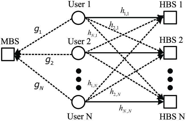
Figure 1: System model of the femtocell network for the uplink transmission.

Under the above framework, for a given time-slot, the uplink transmission for the two-tier femtocell network can be described in Fig. 1. As shown in Fig. 1, user $i$ denotes the scheduled user transmitting to its HBS $\mathcal{B}_{i}$, where $i=1,2,\cdots,N$. All the terminals involved are assumed to be equipped with a single antenna. For the purpose of exposition, all the channels involved are assumed to be block-fading, i.e., the channels remain constant during each transmission block, but possibly change from one block to another. The channel power gain of the link between user $i$ and HBS $\mathcal{B}_{j}$ is denoted by $h_{j,i}$. The channel power gain of the link between user $i$ and the MBS is given by $g_{i}$. All the channel power gains are assumed to be independent and identically distributed (i.i.d.) random variables (RVs) each having a continuous probability density function (PDF). The additive noises at HBSs and MBS are assumed to be independent circularly symmetric complex Gaussian (CSCG) RVs, each of which is assumed to have zero mean and variance $\sigma^{2}$.

We consider two practical femtocell channel models: sparsely deployed scenario and densely deployed scenario. For the sparsely deployed scenario, we assume that the mutual interference between the femtocells is neglected. This is because the channel power gain drops sharply with the increasing of the distance between femtocells due to path loss (which is proportional to $d^{-\alpha}$, where $d$ is the distance and $\alpha$ is the path loss exponent). Besides, since femtocells are usually deployed indoor, the penetration loss is also significant. Therefore, it is reasonable to assume that the interference between femtocells can be neglected when the femtocells are sparsely deployed. In practice, this scenario is applicable to the femtocell networks deployed in rural areas where the distances between femtocells are usually large. While for the urban areas, where the femtocells are close to each other and thus the mutual interference between femtocells cannot be ignored, the sparsely deployed scenario may not be suitable. For such situations, we consider the densely deployed scenario that takes the mutual interference between different femtocells into account. Especially, for this scenario, we assume that the aggregate interference at user $i$’s receiver due to all the other femtocell users is bounded, i.e., $\sum_{j=1,j\neq i}^{N}I^{F}_{j}\leq\varepsilon$, where $\varepsilon$ denotes the bound and $I^{F}_{j}$ denotes the power of the interference from femtocell user $j$. This assumption is valid due to the following facts: (i) the cross-femtocell channel power gains are usually very weak due to the penetration loss; and (ii) the peak transmit power of each femtocell user is usually limited due to practical constraints on power amplifiers.

Notation: In this paper, the boldface capital and lowercase letters are used to denote matrices and vectors, respectively. The inequalities for vectors are defined element-wise, i.e., $\boldsymbol{x}\preceq\boldsymbol{y}$ represents $x_{i}\leq y_{i},~{}\forall i$, where $x_{i}$ and $y_{i}$ are the $i$th elements of the vector $\boldsymbol{x}$ and $\boldsymbol{y}$, respectively. The superscript $T$ denotes the transpose operation of a vector.

III Problem Formulation

In this section, we first present the Stackelberg game formulation for the price-based power allocation scheme. Then, the Stackelberg equilibrium of the proposed game is investigated.

III-A Stackelberg Game Formulation

In this paper, we assume that the maximum interference that the MBS can tolerate is $Q$, i.e., the aggregate interference from all the femtocell users should not be larger than $Q$. Mathematically, this can be written as

$$\sum_{i=1}^{N}I_{i}\leq Q,$$ (1)

where $I_{i}$ denotes the power of the interference from femtocell user $i$. This constraint is known as interference power constraint or interference temperature constraint in CRNs.

Different from the cognitive radio studies, in this paper, we assume that such an interference power constraint is imposed at the MBS, which protects itself through pricing the interference from the femtocell users. The Stackelberg game model [20] is thus applied in this scenario. Stackelberg game is a strategic game that consists of a leader and several followers competing with each other on certain resources. The leader moves first and the followers move subsequently. In this paper, we formulate the MBS as the leader, and the femtocell users as the followers. The MBS (leader) imposes a set of prices on per unit of received interference power from each femtocell user. Then, the femtocell users (followers) update their power allocation strategies to maximize their individual utilities based on the assigned interference prices.

Under the above game model, it is easy to observe that the MBS’s objective is to maximize its revenue obtained from selling the interference quota to femtocell users. Mathematically, the revenue of MBS can be calculated by

$$U_{MBS}\left(\boldsymbol{\mu},\boldsymbol{p}\right)=\sum_{i=1}^{N}\mu_{i}I_{i}(p_{i}),$$ (2)

where $\boldsymbol{\mu}$ is the interference price vector with $\boldsymbol{\mu}=[\mu_{1},\mu_{2},\cdots,\mu_{N}]^{T}$, with $\mu_{i}$ denoting the interference price for user $i$; $I_{i}(p_{i})$ is the interference power received from femtocell user $i$, and $\boldsymbol{p}$ is a vector of power levels for femtocell users with $\boldsymbol{p}=[p_{1},p_{2},\cdots,p_{N}]^{T}$. Note that $\forall i$, $p_{i}$ is actually a function of $\mu_{i}$ under the Stackelberg game formulation, which indicates that the amount of the interference quota that each femtocell user is willing to buy is dependent on its assigned interference price. Since the maximum aggregate interference that the MBS can tolerate is limited, the MBS needs to find the optimal interference prices $\boldsymbol{\mu}$ to maximize its revenue within its tolerable aggregate interference margin. This is obtained by solving the following optimization problem:

Problem 3.1:

$$\max_{\boldsymbol{\mu}\succeq\boldsymbol{0}}~{} U_{MBS}\left(\boldsymbol{\mu},\boldsymbol{p}\right),$$ (3)

s.t. $$\sum_{i=1}^{N}I_{i}(p_{i})\leq Q.$$ (4)

At the femtocell users’ side, the received SINR at HBS $\mathcal{B}_{i}$ for user $i$ can be written as

$$\gamma_{i}\left(p_{i},\boldsymbol{p}_{-i}\right)=\frac{p_{i}h_{i,i}}{\sum_{j\neq i}p_{j}h_{i,j}+\sigma_{i}^{2}},\forall i\in\left\{1,2,\cdots,N\right\}.$$ (5)

where $\sigma_{i}^{2}$ is the background noise at HBS $\mathcal{B}_{i}$ taking into account of the interference from the macrocell users, and $\boldsymbol{p}_{-i}$ is a vector of power allocation for all users except user $i$, i.e., $\boldsymbol{p}_{-i}=[p_{1},\cdots,p_{i-1},p_{i+1},\cdots,p_{N}]^{T}$. Without loss of generality, it is assumed for convenience that $\sigma_{i}^{2}=\sigma^{2},\forall i$ in the rest of this paper.

The utility for user $i$ can be defined as

$$U_{i}\left(p_{i},\boldsymbol{p}_{-i},\mu_{i}\right)=\lambda_{i}\log\left(1+\gamma_{i}\left(p_{i},\boldsymbol{p}_{-i}\right)\right)-\mu_{i}I_{i}(p_{i}),$$ (6)

where $\lambda_{i}$ is the utility gain per unit transmission rate for user $i$, and $I_{i}(p_{i})$ is the interference quota that user $i$ intends to buy from the MBS under the interference price $\mu_{i}$ with $I_{i}(p_{i})\triangleq g_{i}p_{i}$. It is observed from (6) that the utility function of each femtocell user consists of two parts: profit and cost. If the femtocell user increases its transmit power, the transmission rate increases, and so does the profit. On the other hand, with the increasing of the transmit power, the femtocell user will definitely cause more interference to the MBS. As a result, it has to buy more interference quota from the MBS, which increases the cost. Therefore, power allocation strategies are needed at the femtocell users to maximize their own utilities. Mathematically, for each user $i$, this problem can be formulated as

Problem 3.2:

$$\max_{p_{i}}~{} U_{i}\left(p_{i},\boldsymbol{p}_{-i},\boldsymbol{\mu}\right),$$ (7)

s.t. $$~{}p_{i}\geq 0.$$ (8)

Problems 3.1 and 3.2 together form a Stackelberg game. The objective of this game is to find the Stackelberg Equilibrium (SE) point(s) from which neither the leader (MBS) nor the followers (femtocell users) have incentives to deviate. The SE for the proposed game is investigated in the following subsection.

III-B Stackelberg Equilibrium

For the proposed Stackelberg game, the SE is defined as follows.

Definition 3.1: Let $\boldsymbol{\mu}^{*}$ be a solution for Problem 3.1 and $p_{i}^{*}$ be a solution for Problem 3.2 of the $i$th user. Then, the point $\left(\boldsymbol{\mu}^{*},\boldsymbol{p}^{*}\right)$ is a SE for the proposed Stackelberg game if for any $\left(\boldsymbol{\mu},\boldsymbol{p}\right)$ with $\boldsymbol{\mu}\succeq\boldsymbol{0}$ and $\boldsymbol{p}\succeq\boldsymbol{0}$, the following conditions are satisfied:

$$U_{MBS}\left(\boldsymbol{\mu}^{*},\boldsymbol{p}^{*}\right) \geq U_{MBS}\left(\boldsymbol{\mu},\boldsymbol{p}^{*}\right),$$ (9)

$$U_{i}\left(p_{i}^{*},\boldsymbol{p}_{-i}^{*},\boldsymbol{\mu}^{*}\right) \geq U_{i}\left(p_{i},\boldsymbol{p}_{-i}^{*},\boldsymbol{\mu}^{*}\right),\forall i.$$ (10)

Generally, the SE for a Stackelberg game can be obtained by finding its subgame perfect Nash Equilibrium (NE). In the proposed game, it is not difficult to see that the femtocell users strictly compete in a noncooperative fashion. Therefore, a noncooperative power control subgame is formulated at the femtocell users’ side. For a noncooperative game, NE is defined as the operating point(s) at which no player can improve utility by changing its strategy unilaterally, assuming everyone else continues to use its current strategy. At the MBS’s side, since there is only one player, the best response of the MBS can be readily obtained by solving Problem 3.1. To achieve this end, the best response functions for the followers (femtocell users) must be obtained first, since the leader (MBS) derives its best response function based on those of the followers or femtocell users. For the proposed game in this paper, the SE can be obtained as follows: For a given $\boldsymbol{\mu}$, Problem 3.2 is solved first. Then, with the obtained best response functions $\boldsymbol{p}^{*}$ of the femtocells, we solve Problem 3.1 for the optimal interference price $\boldsymbol{\mu}^{*}$.

It is not difficult to see that, in the above formulation, we assume that the MBS charges each femtocell user with a different interference price. We thus refer to this pricing scheme as non-uniform pricing. In addition, we consider a special case of this pricing scheme referred to as uniform pricing, in which the MBS charges each femtocell with the same interference price, i.e., $\mu_{i}=\mu,\forall i$. In the following, these two pricing schemes are investigated for the sparsely deployed scenario and the densely deployed scenario, respectively.

IV Sparsely Deployed Scenario

In the sparsely deployed scenario, we assume that the femtocells are sparsely deployed within the macrocell. Under this assumption, the mutual interference between any pair of femtocells is negligible and thus ignored, i.e., $h_{i,j}=0,\forall i\neq j$. In this scenario, since the inter-femtocell interference is ignored, the problem of solving price-based resource allocation is simplified, which enables us to get the closed-form price and power allocation solutions for the formulated Stackelberg game. As will be shown in the next section, these solutions will enlighten us on the power allocation strategies for the more general densely deployed scenario as well.

In this case, SINR given in (5) can be approximated by

$$\gamma_{i}\left(p_{i},\boldsymbol{p}_{-i}\right)\approx\frac{p_{i}h_{i,i}}{\sigma^{2}},\forall i\in\left\{1,2,\cdots,N\right\}.$$ (11)

Next, we consider the two pricing schemes: non-uniform pricing and uniform pricing, respectively. Then, we compare these two schemes, highlight their advantages and disadvantages for implementation, and point out the best situation under which each scheme should be applied.

IV-A Non-Uniform Pricing

For the non-uniform pricing scheme, the MBS sets different interference prices for different femtocell users. If we denote the interference price for user $i$ as $\mu_{i}$, for the sparsely deployed scenario, Problem 3.2 can be simplified as

Problem 4.1:

$$\max_{p_{i}}~{} \lambda_{i}\log\left(1+\frac{p_{i}h_{i,i}}{\sigma^{2}}\right)-\mu_{i}g_{i}p_{i},$$ (12)

s.t. $$~{}p_{i}\geq 0.$$ (13)

It is observed that the objective function is a concave function over $p_{i}$, and the constraint is affine. Thus, Problem 4.1 is a convex optimization problem. For a convex optimization problem, the optimal solution must satisfy the Karush-Kuhn-Tucker (KKT) conditions. Therefore, by solving the KKT conditions, the optimal solution for Problem 4.1 can be easily obtained in the following lemma. Details are omitted for brevity.

Lemma 4.1: For a given interference price $\mu_{i}$, the optimal solution for Problem 4.1 is given by

$$p_{i}^{*}=\left\{\begin{array}[]{ll}\frac{\lambda_{i}}{\mu_{i}g_{i}}-\frac{\sigma^{2}}{h_{i,i}},&~{}\mbox{if}~{}\mu_{i}<\frac{\lambda_{i}h_{i,i}}{g_{i}\sigma^{2}},\\ 0,&~{}\mbox{otherwise}.\end{array}\right.$$ (16)

From Lemma 4.1, it is observed that if the interference price is too high, i.e., $\mu_{i}>\frac{\lambda_{i}h_{i,i}}{g_{i}\sigma^{2}}$, user $i$ will not transmit. This indicates that user $i$ will be removed from the game.

We can rewrite the power allocation strategy given in (16) as

$$p_{i}^{*}=\left(\frac{\lambda_{i}}{\mu_{i}g_{i}}-\frac{\sigma^{2}}{h_{i,i}}\right)^{+},~{}\forall i,$$ (17)

with $\left(\cdot\right)^{+}\triangleq\max\left(\cdot,0\right)$. Substituting (17) into Problem 3.1, the optimization problem at the MBS side can be formulated as

Problem 4.2:

$$\max_{\boldsymbol{\mu}\succcurlyeq\boldsymbol{0}}~{} \sum_{i=1}^{N}\left(\lambda_{i}-\frac{\mu_{i}g_{i}\sigma^{2}}{h_{i,i}}\right)^{+},$$ (18)

s.t. $$\sum_{i=1}^{N}\left(\frac{\lambda_{i}}{\mu_{i}}-\frac{g_{i}\sigma^{2}}{h_{i,i}}\right)^{+}\leq Q.$$ (19)

Note that the above problem is non-convex, since the object function is a convex function of $\boldsymbol{\mu}$ (maximization of a convex function is in general non-convex). Nevertheless, it is shown in the following that this problem can be converted to a series of convex subproblems.

For user $i$, we introduce the following indicator function

$$\chi_{i}=\left\{\begin{array}[]{cl}1,&\mbox{if}~{}~{}\mu_{i}<\frac{\lambda_{i}h_{i,i}}{g_{i}\sigma^{2}},\\ 0,&\mbox{otherwise}.\end{array}\right.$$ (22)

With the above indicator functions for $i=1,2,\cdots,N$, Problem 4.2 can be reformulated as

Problem 4.3:

$$\max_{\boldsymbol{\chi},~{}\boldsymbol{\mu}\succcurlyeq\boldsymbol{0}}~{} \sum_{i=1}^{N}\chi_{i}\left(\lambda_{i}-\frac{\mu_{i}g_{i}\sigma^{2}}{h_{i,i}}\right),$$ (23)

s.t. $$\sum_{i=1}^{N}\chi_{i}\left(\frac{\lambda_{i}}{\mu_{i}}-\frac{g_{i}\sigma^{2}}{h_{i,i}}\right)\leq Q,$$ (24)

$$~{}\chi_{i}\in\{0,1\},\forall i,$$ (25)

where $\boldsymbol{\chi}\triangleq[\chi_{1},\chi_{2},\cdots,\chi_{N}]^{T}$. It is not difficult to see that the above problem is non-convex due to $\boldsymbol{\chi}$. However, this problem has a nice property that is explored as follows. For a given indicator vector $\boldsymbol{\chi}$, it is easy to verify that Problem 4.3 is convex.

Next, we consider a special case of Problem 4.3 by assuming that $Q$ is large enough such that all the users are admitted. As a result, the indicators for all users are equal to 1, i.e., $\mu_{i}<\frac{\lambda_{i}h_{i,i}}{g_{i}\sigma^{2}},\forall~{}i.$ Under this assumption, Problem 4.3 can be transformed to the following form

Problem 4.4:

$$\min_{\boldsymbol{\mu}\succcurlyeq\boldsymbol{0}}~{} \sum_{i=1}^{N}\frac{\mu_{i}g_{i}\sigma^{2}}{h_{i,i}},$$ (26)

s.t. $$\sum_{i=1}^{N}\frac{\lambda_{i}}{\mu_{i}}\leq Q+\sum_{i=1}^{N}\frac{g_{i}\sigma^{2}}{h_{i,i}}.$$ (27)

Obviously, this problem is convex. The optimal solution of this problem is given by the following proposition.

Proposition 4.1: The optimal solution to Problem 4.4 is given by

$$\mu_{i}^{*}=\sqrt{\frac{\lambda_{i}h_{i,i}}{g_{i}\sigma^{2}}}\frac{\sum_{i=1}^{N}\sqrt{\frac{\lambda_{i}g_{i}\sigma^{2}}{h_{i,i}}}}{Q+\sum_{i=1}^{N}\frac{g_{i}\sigma^{2}}{h_{i,i}}},\forall i\in\left\{1,2,\cdots,N\right\}.$$ (28)

Proof:

Please refer to Part A of the appendix. ∎

Now, we relate the optimal solution of Problem 4.4 to that of the original problem, i.e., Problem 4.2, in the following proposition.

Proposition 4.2: The interference prices given by (28) are the optimal solutions of Problem 4.2 if and only if (iff) $Q>\frac{\sum_{i=1}^{N}\sqrt{\frac{\lambda_{i}g_{i}\sigma^{2}}{h_{i,i}}}}{\min_{i}\sqrt{\frac{\lambda_{i}h_{i,i}}{g_{i}\sigma^{2}}}}-\sum_{i=1}^{N}\frac{g_{i}\sigma^{2}}{h_{i,i}}.$

Proof:

Please refer to Part B of the appendix. ∎

With the results obtained above, we are now ready for solving Problem 4.2. The optimal solution of Problem 4.2 is given in the following theorem.

Theorem 4.1: Assuming that all the femtocell users are sorted in the order $\frac{\lambda_{1}h_{1,1}}{g_{1}\sigma^{2}}>\cdots>\frac{\lambda_{N-1}h_{{N-1},{N-1}}}{g_{N-1}\sigma^{2}}>\frac{\lambda_{N}h_{N,N}}{g_{N}\sigma^{2}}$, the optimal solution for Problem 4.2 is given by

$$\boldsymbol{\mu}^{*}=\left\{\begin{array}[]{cl}\frac{\sum_{i=1}^{N}\sqrt{\frac{\lambda_{i}g_{i}\sigma^{2}}{h_{i,i}}}}{Q+\sum_{i=1}^{N}\frac{g_{i}\sigma^{2}}{h_{i,i}}}[\sqrt{\frac{\lambda_{1}h_{1,1}}{g_{1}\sigma^{2}}},\sqrt{\frac{\lambda_{2}h_{2,2}}{g_{2}\sigma^{2}}},\cdots,\sqrt{\frac{\lambda_{N}h_{N,N}}{g_{N}\sigma^{2}}}]^{T},&\mbox{if}\quad Q>T_{N}\\ \frac{\sum_{i=1}^{N-1}\sqrt{\frac{\lambda_{i}g_{i}\sigma^{2}}{h_{i,i}}}}{Q+\sum_{i=1}^{N-1}\frac{g_{i}\sigma^{2}}{h_{i,i}}}[\sqrt{\frac{\lambda_{1}h_{1,1}}{g_{1}\sigma^{2}}},\cdots,\sqrt{\frac{\lambda_{N-1}h_{N-1,N-1}}{g_{N-1}\sigma^{2}}},\infty]^{T},&\mbox{if}\quad T_{N}\geq Q>T_{N-1}\\ \vdots&\vdots\\ \frac{\sum_{i=1}^{2}\sqrt{\frac{\lambda_{i}g_{i}\sigma^{2}}{h_{i,i}}}}{Q+\sum_{i=1}^{2}\frac{g_{i}\sigma^{2}}{h_{i,i}}}[\sqrt{\frac{\lambda_{1}h_{1,1}}{g_{1}\sigma^{2}}},\sqrt{\frac{\lambda_{2}h_{2,2}}{g_{2}\sigma^{2}}},\infty,\cdots,\infty]^{T},&\mbox{if}\quad T_{3}\geq Q>T_{2}\\ \frac{\sqrt{\frac{\lambda_{1}g_{1}\sigma^{2}}{h_{1,1}}}}{Q+\frac{g_{1}\sigma^{2}}{h_{1,1}}}[\sqrt{\frac{\lambda_{1}h_{1,1}}{g_{1}\sigma^{2}}},\infty,\cdots,\infty]^{T},&\mbox{if}\quad T_{2}\geq Q>T_{1}\end{array}\right.,$$ (34)

where $T_{N}=\frac{\sum_{i=1}^{N}\sqrt{\frac{\lambda_{i}g_{i}\sigma^{2}}{h_{i,i}}}}{\sqrt{\frac{\lambda_{N}h_{N,N}}{g_{N}\sigma^{2}}}}-\sum_{i=1}^{N}\frac{g_{i}\sigma^{2}}{h_{i,i}}$, $T_{N-1}=\frac{\sum_{i=1}^{N-1}\sqrt{\frac{\lambda_{i}g_{i}\sigma^{2}}{h_{i,i}}}}{\sqrt{\frac{\lambda_{N-1}h_{N-1,N-1}}{g_{N-1}\sigma^{2}}}}-\sum_{i=1}^{N-1}\frac{g_{i}\sigma^{2}}{h_{i,i}}$, $\cdots$, $T_{2}=\frac{\sum_{i=1}^{2}\sqrt{\frac{\lambda_{i}g_{i}\sigma^{2}}{h_{i,i}}}}{\sqrt{\frac{\lambda_{2}h_{2,2}}{g_{2}\sigma^{2}}}}-\sum_{i=1}^{2}\frac{g_{i}\sigma^{2}}{h_{i,i}}$, and $T_{1}=\frac{\sqrt{\frac{\lambda_{1}g_{1}\sigma^{2}}{h_{1,1}}}}{\sqrt{\frac{\lambda_{1}h_{1,1}}{g_{1}\sigma^{2}}}}-\frac{g_{1}\sigma^{2}}{h_{1,1}}=0$.

Proof:

If $Q>T_{N}$, the optimal $\boldsymbol{\mu}^{*}$ is readily obtained by Proposition 4.2. For other intervals of $Q$, e.g., $T_{N-1}\leq Q\leq T_{N}$, the proof of the optimality for the corresponding $\boldsymbol{\mu}^{*}$ can be obtained similarly as Proposition 4.2, and is thus omitted. The proof of Theorem 4.1 thus follows. ∎

Remark: From the system design perspective, the results given in (34) are very useful in practice. For instance, if the MBS sets the interference price for a user to $\infty$, this user will not transmit; however, if the system is designed to admit all the $N$ femtocell users, the interference tolerance margin $Q$ at the MBS needs to be set to be above $T_{N}$.

Now, the Stackelberg game for the sparsely deployed scenario with non-uniform pricing is completely solved. The SE for this Stackelberg game is then given as follows.

Proposition 4.3: The SE for the Stackelberg game formulated in Problems 4.1 and 4.2 is $\left(\boldsymbol{\mu}^{*},\boldsymbol{p}^{*}\right)$, where $\boldsymbol{\mu}^{*}$ is given by (34), and $\boldsymbol{p}^{*}$ is given by (16).

In practice, the proposed game can be implemented as follows.

First, for any femtocell user $i$, the MBS measures its channel gain, $g_{i}$, and collects other information such as $\lambda_{i}$ and $h_{i,i}$, from HBS $i$ through the backhaul link. The MBS then computes $\frac{\lambda_{i}h_{i,i}}{g_{i}\sigma^{2}}$ for all $i$’s and use them to compute the threshold vector $\boldsymbol{T}=[T_{N},T_{N-1},\cdots,T_{1}]^{T}$ by Theorem 4.1.

Second, with the obtained threshold vector $\boldsymbol{T}$, the MBS decides the interference price for each femtocell user based on its available interference margin $Q$ according to (34). Then, the interference prices are fed back to femtocell users through the backhaul links between the MBS and the HBSs.

Finally, after receiving the interference prices from their respective HBSs, the femtocell users decide their transmit power levels according to (16).

Moreover, based on the special structure of (34), we propose the following algorithm to compute the interference prices for the femtocell users at the MBS.

Algorithm 4.1: Successive User Removal

• Step 1: Set $K=N$.

• Step 2: Sort the $K$ users according to $\frac{\lambda_{i}h_{i,i}}{g_{i}\sigma^{2}}$ (i.e., $\frac{\lambda_{1}h_{1,1}}{g_{1}\sigma^{2}}>\cdots>\frac{\lambda_{K-1}h_{{K-1},{K-1}}}{g_{K-1}\sigma^{2}}>\frac{\lambda_{K}h_{K,K}}{g_{K}\sigma^{2}}$).

• Step 3: Compute $q_{K}=\frac{\sum_{i=1}^{N}\sqrt{\frac{\lambda_{i}g_{i}\sigma^{2}}{h_{i,i}}}}{Q+\sum_{i=1}^{N}\frac{g_{i}\sigma^{2}}{h_{i,i}}}.$

• Step 4: Comparing the $q_{K}$ with $\sqrt{\frac{\lambda_{K}h_{K,K}}{g_{K}\sigma^{2}}}$. If $q_{K}>\sqrt{\frac{\lambda_{K}h_{K,K}}{g_{K}\sigma^{2}}}$, remove user $K$ from the game, set $K=K-1$, and go to Step 3; otherwise, go to Step 5.

• Step 5: With $q_{K}$ and $K$, the interference price $\mu_{i}$ for user $i$ is given by

  $$\mu_{i}=\left\{\begin{array}[]{ll}q_{K}\sqrt{\frac{\lambda_{i}h_{i,i}}{g_{i}\sigma^{2}}},&\mbox{if}~{}i\leq K\\ \infty,&\mbox{otherwise.}\end{array}\right.$$ (37)

It is observed from the above algorithm that, to obtain the optimal interference price vector $\boldsymbol{\mu}^{*}$, the MBS has to measure and collect the network state information to compute $\frac{\lambda_{i}h_{i,i}}{g_{i}\sigma^{2}}$ for each individual femtocell user $i$. This will incur great implementation complexity and feedback overhead for the MBS and the HBSs. To relieve this burden, we must reduce the amount of information that needs to be known at the MBS. In the following, we consider the uniform pricing scheme, for which the MBS only needs to measure the total received interference power $\sum_{i=1}^{N}I_{i}(p_{i})$ from all the femtocell users to compute the optimal interference price, via a new distributed interference price bargaining algorithm.

IV-B Uniform Pricing

For the uniform pricing scheme, the MBS sets a uniform interference price for all the femtocell users, i.e., $\mu_{i}=\mu,\forall i$. With a uniform price $\mu$, the optimal power allocation for femtocell users can be easily obtained from (16) by setting $\mu_{i}=\mu$, i.e.,

$$p_{i}^{*}=\left(\frac{\lambda_{i}}{\mu g_{i}}-\frac{\sigma^{2}}{h_{i,i}}\right)^{+},~{}\forall i.$$ (38)

Then, at the MBS’s side, the optimization problem reduces to

Problem 4.5:

$$\max_{\mu>0}~{} \sum_{i=1}^{N}\left(\lambda_{i}-\frac{\mu g_{i}\sigma^{2}}{h_{i,i}}\right)^{+},$$ (39)

s.t. $$\sum_{i=1}^{N}\left(\frac{\lambda_{i}}{\mu}-\frac{g_{i}\sigma^{2}}{h_{i,i}}\right)^{+}\leq Q.$$ (40)

This problem has the same structure as Problem 4.2. Therefore, it can be solved by the same method for Problem 4.2. Details are thus omitted here for brevity.

Corollary 4.1: Assuming that all the users are sorted in the order $\frac{\lambda_{1}h_{1,1}}{g_{1}\sigma^{2}}>\cdots>\frac{\lambda_{N-1}h_{{N-1},{N-1}}}{g_{N-1}\sigma^{2}}>\frac{\lambda_{N}h_{N,N}}{g_{N}\sigma^{2}}$, the optimal solution for Problem 4.5 is given by

$$\mu^{*}=\left\{\begin{array}[]{cl}\frac{\sum_{i=1}^{N}\lambda_{i}}{Q+\sum_{i=1}^{N}\frac{g_{i}\sigma^{2}}{h_{i,i}}},&\mbox{if}\quad Q>\tilde{T}_{N}\\ \frac{\sum_{i=1}^{N-1}\lambda_{i}}{Q+\sum_{i=1}^{N-1}\frac{g_{i}\sigma^{2}}{h_{i,i}}},&\mbox{if}\quad\tilde{T}_{N}\geq Q>\tilde{T}_{N-1}\\ \vdots&\vdots\\ \frac{\lambda_{1}}{Q+\frac{g_{1}\sigma^{2}}{h_{1,1}}},&\mbox{if}\quad\tilde{T}_{2}\geq Q>\tilde{T}_{1},\end{array}\right.$$ (45)

where $\tilde{T}_{N}=\frac{\sum_{i=1}^{N}\lambda_{i}}{\frac{\lambda_{N}h_{N,N}}{g_{N}\sigma^{2}}}-\sum_{i=1}^{N}\frac{g_{i}\sigma^{2}}{h_{i,i}}$, $\tilde{T}_{N-1}=\frac{\sum_{i=1}^{N-1}\lambda_{i}}{\frac{\lambda_{N-1}h_{N-1,N-1}}{g_{N-1}\sigma^{2}}}-\sum_{i=1}^{N-1}\frac{g_{i}\sigma^{2}}{h_{i,i}}$, $\cdots$, $\tilde{T}_{2}=\frac{\sum_{i=1}^{2}\lambda_{i}}{\frac{\lambda_{2}h_{2,2}}{g_{2}\sigma^{2}}}-\sum_{i=1}^{2}\frac{g_{i}\sigma^{2}}{h_{i,i}}$, and $\tilde{T}_{1}=\frac{\lambda_{1}}{\frac{\lambda_{1}h_{1,1}}{g_{1}\sigma^{2}}}-\frac{g_{1}\sigma^{2}}{h_{1,1}}=0$.

From Corollary 4.1, it is not to difficult to observe that the optimal price $\mu^{*}$ is unique for a given $Q$. Consequently, the SE for this Stackelberg game is unique and given as follows.

Corollary 4.2: The SE for the Stackelberg game for the uniform pricing case is $\left(\mu^{*},\boldsymbol{p}^{*}\right)$, where $\mu^{*}$ is given by (45), and $\boldsymbol{p}^{*}$ is given by (38).

In practice, the Stackelberg game for the uniform-pricing case can be implemented in the same centralized way as that for the non-uniform pricing case, which requires the MBS to collect a large amount of information from each femtocell user. However, Problem 4.5 has some nice properties that can be explored for the algorithm design. It is observed from Problem 4.5 that both the objective function and the left hand side of (40) are monotonically decreasing functions of $\mu$. Therefore, the objective function is maximized iff (40) is satisfied with equality. By exploiting this fact, we propose the following algorithm to achieve the SE of the Stackelberg game in the unform-pricing case.

Algorithm 4.2: Distributed Interference Price Bargaining

• Step 1: The MBS initializes the interference price $\mu$, and broadcasts $\mu$ to all the femtocell users (e.g., through the HBSs via the backhaul links).

• Step 2: Each femtocell user calculates its optimal transmit power $p^{*}_{i}$ based on the received $\mu$ by (38), and attempts to transmit with $p^{*}_{i}$.

• Step 3: The MBS measures the total received interference $\sum_{i=1}^{N}I_{i}(p_{i})$, and updates the interference price $\mu$ based on $\sum_{i=1}^{N}I_{i}(p_{i})$. Assume that $\epsilon$ is a small positive constant that controls the algorithm accuracy. Then, if $\sum_{i=1}^{N}I_{i}(p_{i})>Q+\epsilon$, the MBS increases the interference price by $\Delta\mu$; if $\sum_{i=1}^{N}I_{i}(p_{i})<Q-\epsilon$, the MBS decreases the interference price by $\Delta\mu$, where $\Delta\mu>0$ is a small step size. After that, the MBS broadcasts the new interference price to all the femtocells users.

• Step 4: Step 2 and Step 3 are repeated until $\big{|}\sum_{i=1}^{N}I_{i}(p_{i})-Q\big{|}\leq\epsilon$.

Remark: The convergence of Algorithm 4.2 is guaranteed due to the following facts: (i) the optimal $\mu$ is obtained when (40) is satisfied with equality; and (ii) the left hand side of (40) is a monotonically decreasing function of $\mu$.

It is seen that Algorithm 4.2 is a distributed algorithm. At the MBS side, the MBS only needs to measure the total received interference $\sum_{i=1}^{N}I_{i}(p_{i})$. At the femtocell side, each femtocell user only needs to know the channel gain to its own HBS to compute the transmit power. Overall, the amount of information that needs to be exchanged in the network is greatly reduced, as compared to the centralized approach.

IV-C Non-Uniform Pricing vs. Uniform Pricing

In the following, we summarize the main results on comparing the two schemes of non-uniform pricing and uniform pricing.

First, it is observed that the non-uniform pricing scheme must be implemented in a centralized way, while the uniform pricing scheme can be implemented in a decentralized way. Therefore, uniform pricing is more favorable when the network state information is not available.

Secondly, the non-uniform pricing scheme maximizes the revenue of the MBS, while the uniform pricing scheme maximizes the sum-rate of the femtocell users. It is easy to observe that non-uniform pricing is optimal from the perspective of revenue maximization of the MBS, as compared to uniform pricing. However, it is not immediately clear that the uniform pricing scheme is indeed optimal for the sum-rate maximization of the femtocell users. Hence, the following proposition affirms this property.

Proposition 4.4: For a given interference power constraint $Q$, the sum-rate of the femtocell users is maximized by the uniform pricing scheme.

Proof:

Please refer to Part C of the appendix. ∎

V Densely Deployed Scenario

In this scenario, we assume that the femtocells are densely deployed within the region covered by the macrocell. Therefore, the mutual interference between femtocells cannot be neglected. However, as previously stated in the system model, it is still reasonable to assume that the aggregate interference at user $i$’s receiver due to all other femtocell users is bounded, i.e., $\sum_{j\neq i}p_{j}^{*}h_{i,j}\leq\varepsilon$, where $\varepsilon$ denotes the upper bound.

For this scenario, we also consider two pricing schemes: non-uniform pricing and uniform pricing, which are studied in the following two subsections, respectively.

V-A Non-Uniform Pricing

Under the non-uniform pricing scheme, the MBS sets different interference prices for different femtocell users. If we denote the interference price for user $i$ as $\mu_{i}$, the best responses for the noncooperative game at the femtocell users’ side can be obtained by solving Problem 3.2 as follows.

For given $\boldsymbol{p}_{-i}$ and $\mu_{i}$, it is easy to verify that Problem 3.2 is a convex optimization problem. Thus, the best response function for user $i$ can be obtained by setting $\frac{\partial U_{i}\left(p_{i},\boldsymbol{p}_{-i},\mu_{i}\right)}{\partial p_{i}}$ to $0$. Taking the first-order derivative of (6), we have

$$\frac{\partial U_{i}\left(p_{i},\boldsymbol{p}_{-i},\mu_{i}\right)}{\partial p_{i}}=\frac{\lambda_{i}}{\frac{p_{i}}{\gamma_{i}\left(p_{i},\boldsymbol{p}_{-i}\right)}+p_{i}}-\mu_{i}g_{i}=0.$$ (46)

Substituting the $\gamma_{i}\left(p_{i},\boldsymbol{p}_{-i}\right)$ given in (5) into (46) yields

$$p_{i}^{*}=\left(\frac{\lambda_{i}}{\mu_{i}g_{i}}-\frac{\sum_{j\neq i}p_{j}^{*}h_{i,j}+\sigma^{2}}{h_{i,i}}\right)^{+},\forall i\in\left\{1,2,\cdots,N\right\}.$$ (47)

For a given interference vector $\boldsymbol{\mu}$, (47) represents an $N$-user non-cooperative game. It is easy to verify that, for a given interference vector $\boldsymbol{\mu}$, there exists at least one NE for the non-cooperative game defined by (47). In general, there are multiple NEs, and thus it is NP-hard to get the optimal power allocation vector $\boldsymbol{p}^{*}$.

Fortunately, since the aggregate interference is bounded, we may consider first the worst case, i.e., $\sum_{j\neq i}p_{j}^{*}h_{i,j}=\varepsilon$, $\forall i$. In this case, the best response functions of all users are decoupled in terms of $p_{i}$’s. If we denote $\varepsilon+\sigma^{2}$ as $\theta$, the revenue maximization problem at the MBS’s side will be exactly the same as Problem 4.2, with $\sigma^{2}$ replaced by $\theta$. Therefore, the optimal interference price vectors can be obtained by Theorem 4.1, with $\sigma^{2}$ replaced by $\theta$.

On the other hand, we may also consider the ideal case, i.e., $\sum_{j\neq i}p_{j}^{*}h_{i,j}=0$, $\forall i$. Then, the revenue maximization problem at the MBS’s side will be exactly the same as Problem 4.2, and the optimal interference price vector can be obtained by Theorem 4.1.

It is observed that the method used to solve the sparsely deployed scenario can be directly applied to solve the densely deployed scenario by considering the worst case and the ideal case, respectively. It is not difficult to show that the worst case and the ideal case serve as the lower bound and the upper bound on the maximum achievable revenue of the MBS, respectively. Furthermore, these bounds will get closer to each other with the decreasing of $\varepsilon$ and eventually collide when $\varepsilon=0$.

V-B Uniform Pricing

Under the uniform pricing scheme with $\mu_{i}=\mu,\forall i$, the optimal power allocation for femtocell users can be easily obtained from (47) as

$$p_{i}^{*}=\left(\frac{\lambda_{i}}{\mu g_{i}}-\frac{\sum_{j\neq i}p_{j}^{*}h_{i,j}+\sigma^{2}}{h_{i,i}}\right)^{+},\forall i\in\left\{1,2,\cdots,N\right\}.$$ (48)

Again, it is NP-hard to get the optimal power allocation vector $\boldsymbol{p}^{*}$. Similarly, we can solve this problem by either considering the worst case or the ideal case, for both of which the methods used to solve the sparsely deployed scenario can be directly applied. Details are thus omitted for brevity. Last, it is worth noting that the distributed interference price bargaining algorithm (Algorithm 4.2) can also be applied in the case of $\varepsilon>0$; however, the convergence of this algorithm is no more guaranteed due to the non-uniqueness of NE solutions for the non-cooperate power game in (48). Nevertheless, the convergence of this algorithm is usually observed in our numerical experiments when $\varepsilon$ is sufficiently small.

VI Numerical Results

In this section, several numerical examples are provided to evaluate the performances of the proposed resource allocation strategies based on the approach of interference pricing. For simplicity, we assume that the variance of the noise is 1, and the payoff factors $\lambda_{i},\forall i$ are all equal to 1.

A two-tier spectrum-sharing femtocell network with one MBS and three femtocells is considered. Without loss of generality, the channel power gains are chosen as follows: $h_{1,1}=1$, $h_{2,2}=1$, $h_{3,3}=1$, $g_{1}=0.01$, $g_{2}=0.1$, and $g_{3}=1$. In the following, the first three examples are for the sparsely deployed scenario, while the last one is for the densely deployed scenario.

VI-A Example 1: Uniform Pricing vs. Non-Uniform Pricing: Throughput-Revenue Tradeoff

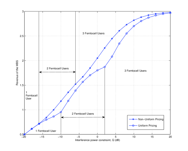
Figure 2: Revenue of the MBS vs. $Q$.

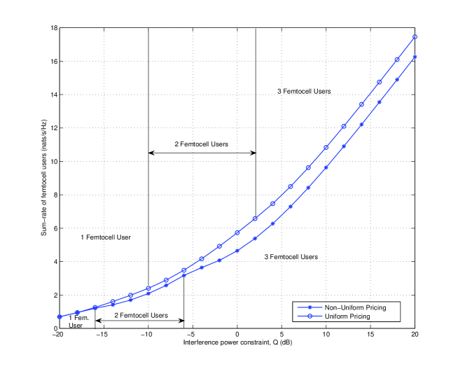
Figure 3: Sum-rate of femtocell users vs. $Q$.

Figs. 2 and 3 show the macrocell revenue and the sum-rate of femtocell users, respectively, versus the maximum tolerable interference margin $Q$ at the MBS, with uniform or non-uniform pricing. It is observed that for the same $Q$, the revenue of the MBS under the non-uniform pricing scheme is in general larger than that under the uniform pricing scheme, while the reverse is generally true for the sum-rate of femtocell users. These observations are in accordance with our discussions given in Section IV. In addition, it is worth noting that when $Q$ is sufficiently small, the revenues of the MBS become equal for the two pricing schemes, so are the sum-rates of femtocell users. This is because when $Q$ is very small, there is only one femtocell active in the network, and thus by comparing (34) and (45), the non-uniform pricing scheme is same as the uniform pricing counterpart in the single-femtocell case. It is also observed that when $Q$ is sufficiently large, the revenues of the MBS converge to the same value for the two pricing schemes. This can be explained as follows. For the non-uniform pricing scheme, when $Q$ is very large, it is observed from (34) that $\mu_{i}$’s all become very small, and thus the objective function of Problem 4.2 converges to $\sum_{i=1}^{N}\lambda_{i}$ as $Q\rightarrow\infty$. On the other hand, for the uniform pricing scheme, the revenue of the MBS can be written as $\mu^{*}Q$ at the optimal point, which is equal to $\frac{Q\sum_{i=1}^{N}\lambda_{i}}{Q+\sum_{i=1}^{N}\frac{g_{i}\sigma^{2}}{h_{i,i}}}$ when $Q$ is very large (cf. (45)). Clearly, this value will converge to $\sum_{i=1}^{N}\lambda_{i}$ as $Q\rightarrow\infty$.

VI-B Example 2: Comparison of Interference Prices of Femtocell Users under Non-Uniform Pricing

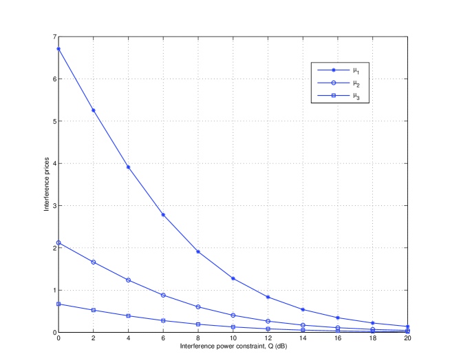
Figure 4: Interference prices for femtocell users vs. $Q$ under non-uniform pricing.

In this example, we examine the optimal interference prices of the femtocell users vs. $Q$ under non-uniform pricing. First, it is observed from Fig. 4 that, for the same $Q$, the interference price for femtocell user $1$ is the highest, while that for femtocell user $3$ is the lowest. This is true due the fact that $\frac{\lambda_{1}h_{1,1}}{g_{1}\sigma^{2}}>\frac{\lambda_{2}h_{2,2}}{g_{2}\sigma^{2}}>\frac{\lambda_{3}h_{3,3}}{g_{3}\sigma^{2}}$, where a larger $\frac{\lambda_{i}h_{i,i}}{g_{i}\sigma^{2}}$ indicates that the corresponding femtocell can achieve a higher profit (transmission rate) with the same amount network resource (transmit power) consumed. Therefore, the user with a larger $\frac{\lambda_{i}h_{i,i}}{g_{i}\sigma^{2}}$ has a willingness to pay a higher price to consume the network resource. Secondly, it is observed that the differences between the interference prices decrease with the increasing of $Q$. This is due to the fact that $\frac{\sum_{i=1}^{N}\sqrt{\frac{\lambda_{i}g_{i}\sigma^{2}}{h_{i,i}}}}{Q+\sum_{i=1}^{N}\frac{g_{i}\sigma^{2}}{h_{i,i}}}$ in (34) decreases with the increasing of $Q$. Lastly, it is observed that the interference prices for all femtocell users decrease with the increasing of $Q$, which can be easily inferred from (34). Intuitively, this can be explained by the practical rule of thumb that a seller would like to price lower if it has a large amount of goods to sell.

VI-C Example 3: Convergence Performance of Distributed Interference Price Bargaining Algorithm

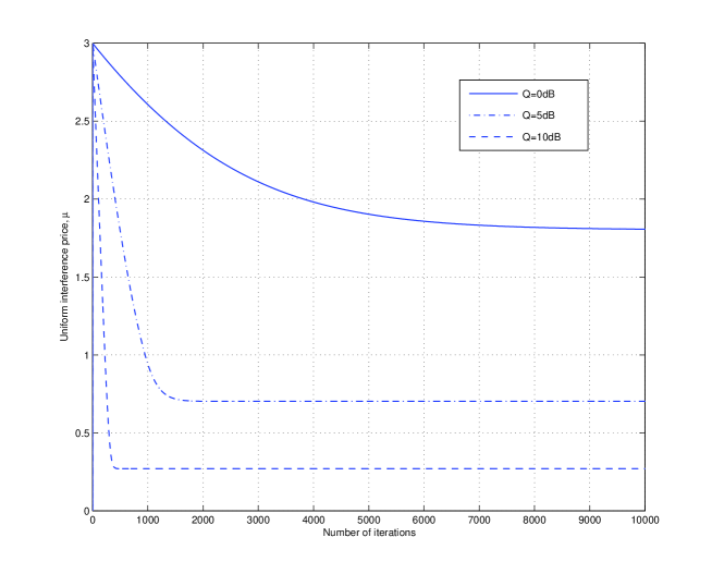
Figure 5: Convergence performance of the distributed interference price bargaining algorithm with the subgradient search.

In this example, we investigate the convergence performance of the distributed interference price bargaining algorithm (Algorithm 4.2). The initial value of $\mu$ is chosen to be $0.001$. The $\Delta\mu$ is chosen to be $0.001\times|\sum_{i=1}^{N}I_{i}(p_{i})-Q|$. The desired accuracy $\epsilon$ is chosen to be $10^{-6}$. It is observed from Fig. 5 that the distributed bargaining algorithm converges for all values of $Q$. It is also observed that the convergence speed increases with the increasing of $Q$. This is because $\Delta\mu$ is proportional to $|\sum_{i=1}^{N}I_{i}(p_{i})-Q|$, i.e., increasing $Q$ is equivalent to increasing the step size $\Delta\mu$, and consequently increases the convergence speed.

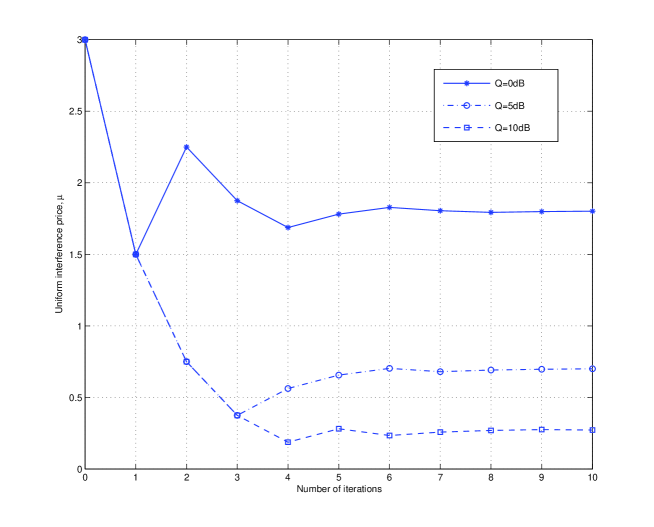
Figure 6: Convergence performance of the distributed interference price bargaining algorithm with the bisection search.

Actually, the convergence speed of the distributed bargaining algorithm can be greatly improved by implementing it by the bisection method, for which the implementation procedure is as follows. First, the MBS initializes a lower bound $\mu_{L}$ and an upper bound $\mu_{H}$ of the interference price. Then, the MBS computes $\mu_{M}=(\mu_{L}+\mu_{H})/2$ and broadcasts $\mu_{M}$ to femtocell users. Receiving $\mu_{M}$, femtocell users compute their optimal transmit power and then transmit with the computed power. The MBS then measures the total received interference $\sum_{i=1}^{N}I_{i}(p_{i})$ from femtocell users. If $\sum_{i=1}^{N}I_{i}(p_{i})<Q$, the MBS sets $\mu_{H}=\mu_{M}$; otherwise, the MBS sets $\mu_{L}=\mu_{M}$. Then, $\mu_{M}$ is recomputed based on the new lower and upper bounds. The algorithm stops when $|\sum_{i=1}^{N}I_{i}(p_{i})-Q|$ is within the desired accuracy. It is observed from Fig. 6 that the bisection method converges much faster than the simple subgradient-based method in Fig. 5.

VI-D Example 4: Densely Deployed Scenario under Unform Pricing

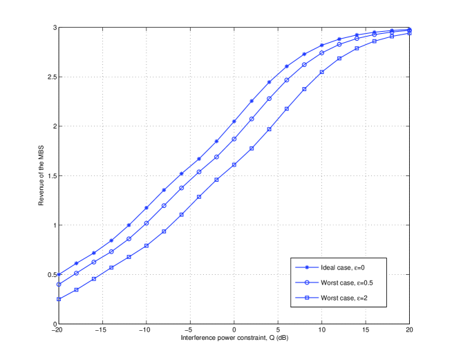
Figure 7: Revenue of the MBS vs. $Q$ for the densely deployed scenario.

In this example, we investigate the macrocell revenue for the densely deployed scenario under uniform pricing. First, it is observed from Fig. 7 that the ideal case of $\varepsilon=0$ has the largest revenue of the MBS, compared to the other two cases with $\varepsilon=0.5,2$. This verifies that the ideal case can serve as a revenue upper bound for the densely deployed scenario. Secondly, the revenues of the MBS for all the three cases of $\varepsilon=0,0.5,2$ increase with the increasing of $Q$, similarly as expected for the sparsely deployed scenario. Lastly, the revenue of the MBS is observed to increase with the decreasing of $\varepsilon$ for the same $Q$, and the revenue differences become smaller as $Q$ increases.

VII Conclusion

In this paper, price-based power allocation strategies are investigated for the uplink transmission in a spectrum-sharing-based two-tier femtocell network using game theory. An interference power constraint is applied to guarantee the quality-of-service (QoS) of the MBS. Then, the Stackelberg game model is adopted to jointly study the utility maximization of the MBS and femtocell users. The optimal resource allocation schemes including the optimal interference prices and the optimal power allocation strategies are examined. Especially, closed-form solutions are obtained for the sparsely deployed scenario. Besides, a distributed algorithm that rapidly converges to the Stackelberg equilibrium is proposed for the uniform pricing scheme. It is shown that the proposed algorithm has a low complexity and requires minimum information exchange between the MBS and femtocell users. The results of this paper will be useful to the practical design of interference control in spectrum-sharing femtocell networks.

Appendix

VII-A Proof of Proposition 4.1

It is easy to observe that Problem 4.4 is a convex optimization problem. Thus, the dual gap between this problem and its dual optimization problem is zero. Therefore, we can solve Problem 4.4 by solving its dual problem.

The Lagrangian associated with Problem 4.4 can be written as

$$\mathcal{L}\left(\boldsymbol{\mu},\alpha,\boldsymbol{\beta}\right)=\sum_{i=1}^{N}\frac{\mu_{i}g_{i}\sigma^{2}}{h_{i,i}}+\alpha\left(\sum_{i=1}^{N}\frac{\lambda_{i}}{\mu_{i}}-Q-\sum_{i=1}^{N}\frac{g_{i}\sigma^{2}}{h_{i,i}}\right)-\sum_{i=1}^{N}\beta_{i}\mu_{i},$$ (49)

where $\alpha$ and $\beta_{i}$ are non-negative dual variables associated with the constraints $\sum_{i=1}^{N}\frac{\lambda_{i}}{\mu_{i}}\leq Q+\sum_{i=1}^{N}\frac{g_{i}\sigma^{2}}{h_{i,i}}$ and $\mu_{i}\geq 0$, respectively.

The dual function is then defined as $\mathcal{G}\left(\boldsymbol{\mu},\alpha,\boldsymbol{\beta}\right)=\max_{\boldsymbol{\mu}\succcurlyeq\boldsymbol{0}}{L}\left(\boldsymbol{\mu},\alpha,\boldsymbol{\beta}\right),$ and the dual problem is given by $\min_{\alpha\geq 0,\boldsymbol{\beta}\succcurlyeq\boldsymbol{0}}\mathcal{G}\left(\boldsymbol{\mu},\alpha,\boldsymbol{\beta}\right).$ Then, the KKT conditions can be written as follows:

$$\frac{\partial{L}\left(\boldsymbol{\mu},\alpha,\boldsymbol{\beta}\right)}{\partial\mu_{i}} =0,\forall i,$$ (50)

$$\alpha\left(\sum_{i=1}^{N}\frac{\lambda_{i}}{\mu_{i}}-Q-\sum_{i=1}^{N}\frac{g_{i}\sigma^{2}}{h_{i,i}}\right) =0,$$ (51)

$$\beta_{i}\mu_{i} =0,\forall i,$$ (52)

$$\alpha \geq 0,$$ (53)

$$\beta_{i} \geq 0,\forall i,$$ (54)

$$\mu_{i} \geq 0,\forall i,$$ (55)

$$\sum_{i=1}^{N}\frac{\lambda_{i}}{\mu_{i}}-Q-\sum_{i=1}^{N}\frac{g_{i}\sigma^{2}}{h_{i,i}} \leq 0.$$ (56)

From (50), we have

$$\frac{\partial{L}\left(\boldsymbol{\mu},\alpha,\boldsymbol{\beta}\right)}{\partial\mu_{i}}=\frac{g_{i}\sigma^{2}}{h_{i,i}}-\alpha\frac{\lambda_{i}}{\mu_{i}^{2}}-\beta_{i},\forall i.$$ (57)

Setting the above function equal to $0$ yields

$$\mu_{i}^{2}=\alpha\frac{\lambda_{i}}{\frac{g_{i}\sigma^{2}}{h_{i,i}}-\beta_{i}},\forall i.$$ (58)

Lemma 1: $\beta_{i}=0,\forall i.$

Proof:

Suppose that $\beta_{i}\neq 0$ for any arbitrary $i$. Then, according to (52), it follows that $\mu_{i}=0$. From (58), we know that $\mu_{i}=0$ indicates that $\alpha=0$, since $\lambda_{i}>0$. Then, from (58), it follows that $\mu_{i}=0,\forall i$, which contradicts (56). Therefore, the preassumption that $\beta_{i}\neq 0$ for any given $i$ does not hold, and we thus have $\beta_{i}=0,\forall i.$ ∎

Lemma 2: $\sum_{i=1}^{N}\frac{\lambda_{i}}{\mu_{i}}-Q-\sum_{i=1}^{N}\frac{g_{i}\sigma^{2}}{h_{i,i}}=0.$

Proof:

Suppose that $\sum_{i=1}^{N}\frac{\lambda_{i}}{\mu_{i}}-Q-\sum_{i=1}^{N}\frac{g_{i}\sigma^{2}}{h_{i,i}}\neq 0.$ Then, from (51), we have $\alpha=0$. Then, from (58), it follows $\mu_{i}=0,\forall i$, which contradicts (56). Therefore, the aforementioned preassumption does not hold, and we have $\sum_{i=1}^{N}\frac{\lambda_{i}}{\mu_{i}}-Q-\sum_{i=1}^{N}\frac{g_{i}\sigma^{2}}{h_{i,i}}=0.$ ∎

According to Lemma 1 and $\mu_{i}\geq 0$, (58) can be rewritten as

$$\mu_{i}=\sqrt{\alpha\frac{\lambda_{i}h_{i,i}}{g_{i}\sigma^{2}}},\forall i.$$ (59)

Substituting the above equation into (41) and according to Lemma 2, we have

$$\sqrt{\alpha}=\frac{\sum_{i=1}^{N}\sqrt{\frac{\lambda_{i}g_{i}\sigma^{2}}{h_{i,i}}}}{Q+\sum_{i=1}^{N}\frac{g_{i}\sigma^{2}}{h_{i,i}}}.$$ (60)

Then, substituting (45) back to (44) yields

$$\mu_{i}=\sqrt{\frac{\lambda_{i}h_{i,i}}{g_{i}\sigma^{2}}}\frac{\sum_{i=1}^{N}\sqrt{\frac{\lambda_{i}g_{i}\sigma^{2}}{h_{i,i}}}}{Q+\sum_{i=1}^{N}\frac{g_{i}\sigma^{2}}{h_{i,i}}}.$$ (61)

Proposition 4.1 is thus proved.

VII-B Proof of Proposition 4.2

First, consider the proof of the “if” part. It is observed that the interference vector $\boldsymbol{\mu}^{*}$ given by (28) is the optimal solution of Problem 4.2 if all the indicator functions are equal to 1, i.e., $\mu_{i}<\frac{\lambda_{i}h_{i,i}}{g_{i}\sigma^{2}},\forall~{}i\in\left\{1,2,\cdots,N\right\}$.

Substituting (28) into the above inequalities yields

$$\sqrt{\frac{\lambda_{i}h_{i,i}}{g_{i}\sigma^{2}}}\frac{\sum_{i=1}^{N}\sqrt{\frac{\lambda_{i}g_{i}\sigma^{2}}{h_{i,i}}}}{Q+\sum_{i=1}^{N}\frac{g_{i}\sigma^{2}}{h_{i,i}}}<\frac{\lambda_{i}h_{i,i}}{g_{i}\sigma^{2}},\forall~{}i\in\left\{1,2,\cdots,N\right\}.$$ (62)

Then, it follows

$$Q>\frac{\sum_{i=1}^{N}\sqrt{\frac{\lambda_{i}g_{i}\sigma^{2}}{h_{i,i}}}}{\sqrt{\frac{\lambda_{i}h_{i,i}}{g_{i}\sigma^{2}}}}-\sum_{i=1}^{N}\frac{g_{i}\sigma^{2}}{h_{i,i}},\forall~{}i\in\left\{1,2,\cdots,N\right\}.$$ (63)

Furthermore, the inequalities given in (63) can be compactly written as

$$Q>\frac{\sum_{i=1}^{N}\sqrt{\frac{\lambda_{i}g_{i}\sigma^{2}}{h_{i,i}}}}{\min_{i}\sqrt{\frac{\lambda_{i}h_{i,i}}{g_{i}\sigma^{2}}}}-\sum_{i=1}^{N}\frac{g_{i}\sigma^{2}}{h_{i,i}}.$$ (64)

The “if” part is thus proved.

Next, consider the “only if” part, which is proved by contradiction as follows.

For the ease of exposition, we assume that femtocell users are sorted by the following order:

$$\frac{\lambda_{1}h_{1,1}}{g_{1}\sigma^{2}}>\cdots>\frac{\lambda_{N-1}h_{{N-1},{N-1}}}{g_{N-1}\sigma^{2}}>\frac{\lambda_{N}h_{N,N}}{g_{N}\sigma^{2}}.$$ (65)

Then, in Proposition 4.2, the condition becomes

$$Q>T_{N},~{}\mbox{where}~{}T_{N}=\frac{\sum_{i=1}^{N}\sqrt{\frac{\lambda_{i}g_{i}\sigma^{2}}{h_{i,i}}}}{\sqrt{\frac{\lambda_{N}h_{N,N}}{g_{N}\sigma^{2}}}}-\sum_{i=1}^{N}\frac{g_{i}\sigma^{2}}{h_{i,i}}.$$ (66)

Now, suppose $T_{N-1}<Q\leq T_{N}$, where $T_{N-1}$ is a threshold shown later in (70). Suppose that $\boldsymbol{\mu}^{*}$ given by (28) is still optimal for Problem 4.2 with $T_{N-1}<Q\leq T_{N}$. Then, since $Q\leq T_{N}$, from (28) it follows that $\mu^{*}_{N}\geq\frac{\lambda_{N}h_{N,N}}{g_{N}\sigma^{2}}$ and thus $\left(\frac{\lambda_{N}}{\mu_{N}^{*}}-\frac{g_{N}\sigma^{2}}{h_{N,N}}\right)^{+}=0$. From Problem 4.2, it then follows that $\mu^{*}_{1},\ldots,\mu^{*}_{N-1}$ must be the optimal solution of the following problem

$$\max_{\boldsymbol{\mu}\succcurlyeq\boldsymbol{0}}~{} \sum_{i=1}^{N-1}\left(\lambda_{i}-\frac{\mu_{i}g_{i}\sigma^{2}}{h_{i,i}}\right)^{+},$$ (67)

s.t. $$\sum_{i=1}^{N-1}\left(\frac{\lambda_{i}}{\mu_{i}}-\frac{g_{i}\sigma^{2}}{h_{i,i}}\right)^{+}\leq Q.$$ (68)

This problem has the same structure as Problem 4.2. Thus, from the proof of the previous “if” part, we can show that the optimal solution for this problem is given by

$$\mu_{i}^{\star}=\sqrt{\frac{\lambda_{i}h_{i,i}}{g_{i}\sigma^{2}}}\frac{\sum_{i=1}^{N-1}\sqrt{\frac{\lambda_{i}g_{i}\sigma^{2}}{h_{i,i}}}}{Q+\sum_{i=1}^{N-1}\frac{g_{i}\sigma^{2}}{h_{i,i}}},\quad\forall i\in\left\{1,2,\cdots,N-1\right\},$$ (69)

if $Q>T_{N-1}$, where $T_{N-1}$ is obtained as the threshold for $Q$ above which $\mu^{\star}_{i}<\frac{\lambda_{i}h_{i,i}}{g_{i}\sigma^{2}}$ holds $\forall i\in\{1,\ldots,N-1\}$, i.e.,

$$T_{N-1}=\frac{\sum_{i=1}^{N-1}\sqrt{\frac{\lambda_{i}g_{i}\sigma^{2}}{h_{i,i}}}}{\sqrt{\frac{\lambda_{N-1}h_{N-1,N-1}}{g_{N-1}\sigma^{2}}}}-\sum_{i=1}^{N-1}\frac{g_{i}\sigma^{2}}{h_{i,i}}.$$ (70)

Obviously, the optimal interference price solution in (69) for the above problem is different from $\boldsymbol{\mu}^{*}$ given by (28). Thus, this contradicts with our presumption that $\boldsymbol{\mu}^{*}$ is optimal for Problem 4.2 with $T_{N-1}<Q\leq T_{N}$. Therefore, the interference vector $\boldsymbol{\mu}^{*}$ given by (28) is the optimal solution of Problem 4.2 only if $Q>T_{N}$. The “only if” part thus follows.

By combining the proofs of both the “if” and “only if” parts, Proposition 4.2 is thus proved.

VII-C Proof of Proposition 4.3

For a given interference power constraint $Q$, the sum-rate maximization problem of the femtocell network can be formulated as

$$\max_{\boldsymbol{p}\succcurlyeq\boldsymbol{0}}~{} \sum_{i=1}^{N}\log\left(1+\frac{h_{i,i}p_{i}}{\sigma_{i}^{2}}\right),$$ (71)

s.t. $$\sum_{i=1}^{N}g_{i}p_{i}\leq Q.$$ (72)

It is easy to observe that the sum-rate optimization problem is a convex optimization problem. The Lagrangian associated with this problem can be written as

$$\mathcal{L}\left(\boldsymbol{p},\nu\right)=\sum_{i=1}^{N}\log\left(1+\frac{h_{i,i}p_{i}}{\sigma_{i}^{2}}\right)-\nu\left(\sum_{i=1}^{N}g_{i}p_{i}-Q\right),$$ (73)

where $\nu$ is the non-negative dual variable associated with the constraint $\sum_{i=1}^{N}g_{i}p_{i}\leq Q$.

The dual function is then defined as $\mathcal{G}\left(\boldsymbol{p},\nu\right)=\max_{\boldsymbol{p}\succcurlyeq\boldsymbol{0}}\mathcal{L}\left(\boldsymbol{p},\nu\right),$ and the dual problem is $\min_{\nu\geq 0}\mathcal{G}\left(\boldsymbol{p},\nu\right).$ For a fixed $\nu$, it is not difficult to observe that the dual function can also be written as

$$\mathcal{G}\left(\boldsymbol{p},\nu\right)=\max_{\boldsymbol{p}\succcurlyeq\boldsymbol{0}}\sum_{i=1}^{N}\tilde{\mathcal{L}}\left(p_{i},\nu\right)+\nu Q,$$ (74)

where

$$\tilde{\mathcal{L}}\left(p_{i},\nu\right)=\log\left(1+\frac{h_{i,i}p_{i}}{\sigma_{i}^{2}}\right)-\nu g_{i}p_{i}.$$ (75)

Thus, the dual function can be obtained by solving a set of independent sub-dual-functions each for one user. This is also known as the “dual decomposition” [19]. For a particular user, the problem can be expressed as

$$\max_{p_{i}>0}~{}\log\left(1+\frac{h_{i,i}p_{i}}{\sigma_{i}^{2}}\right)-\nu g_{i}p_{i}.$$ (76)

It can be seen that the dual variable $\nu$ plays the same role as the uniform price $\mu$. It is easy to observe that these sub-problems are exactly the same as the power allocation problems under the uniform pricing scheme when $\nu=\mu$. Note that for the sum-rate maximization problem, $\nu$ is obtained when the interference constraint is met with equality. Therefore, the optimal dual solution of $\nu$ is guaranteed to converge to $\mu^{*}$ for the formulated Stackelberg game with uniform pricing.

Proposition 4.3 is thus proved.

References

- [1] V. Chandrasekhar, J. G. Andrews, and A. Gatherer, “Femtocell networks: a survey,” IEEE Commun. Mag., vol. 46, no. 9, pp. 59–67, 2008.
- [2] H. Claussen, L. Ho, and L. Samuel, “Self-optimization of coverage for femtocell deployments,” in Wireless Telecommunications Symposium (WTS), 2008, pp. 278 –285.
- [3] V. Chandrasekhar, J. G. Andrews, T. Muharemovic, Z. Shen, and A. Gatherer, “Power control in two-tier femtocell networks,” IEEE Trans. on Wireless Commun., vol. 8, no. 8, pp. 4316–4328, Aug. 2009.
- [4] H.-S. Jo, C. Mun, J. Moon, and J.-G. Yook, “Interference mitigation using uplink power control for two-tier femtocell networks,” IEEE Trans. on Wireless Commun., vol. 8, no. 10, pp. 4906–4910, Oct. 2009.
- [5] D. Lopez-Perez, A. Valcarce, G. de la Roche, and J. Zhang, “Ofdma femtocells: A roadmap on interference avoidance,” IEEE Commun. Mag., vol. 47, no. 9, pp. 41 –48, 2009.
- [6] S. Park, W. Seo, Y. Kim, S. Lim, and D. Hong, “Beam subset selection strategy for interference reduction in two-tier femtocell networks,” IEEE Trans. Wireless Commun., vol. 9, no. 11, pp. 3440–3449, 2010.
- [7] S. Rangan, “Femto-macro cellular interference control with subband scheduling and interference cancelation,” Available at arXiv: 1007.0507.
- [8] Y. Kim, S. Lee, and D. Hong, “Performance analysis of two-tier femtocell networks with outage constraints,” IEEE Trans. Wireless Commun., vol. 9, no. 9, pp. 2695 –2700, 2010.
- [9] L. Giupponi, A. Galindo-Serrano, and M. Dohler, “From cognition to docition: The teaching radio paradigm for distributed and autonomous deployments,” Elsevier Computer Commun., vol. 33, no. 17, pp. 2015 –2020, 2010.
- [10] S. Haykin, “Cognitive radio: brain-empowered wireless communications,” IEEE J. Select. Areas Commun., vol. 23, no. 2, pp. 201–220, Feb. 2005.
- [11] X. Kang, Y.-C. Liang, A. Nallanathan, H. K. Garg, and R. Zhang, “Optimal power allocation for fading channels in cognitive radio networks: Ergodic capacity and outage capacity,” IEEE Trans. on Wireless Commun., vol. 8, no. 2, pp. 940–950, Feb. 2009.
- [12] X. Kang, R. Zhang, Y.-C. Liang, and H. K. Garg, “Optimal power allocation strategies for fading cognitive radio channels with primary user s outage constraint,” IEEE J. Select. Areas Commun., vol. 29, no. 2, pp. 374–383, Feb. 2011.
- [13] K. Huang, V. K. N. Lau, and Y. Chen, “Spectrum sharing between cellular and mobile ad hoc networks: transmission-capacity trade-off,” IEEE J. Select. Areas Commun., vol. 27, no. 7, pp. 1256–1267, Sept. 2009.
- [14] L. Gao and S. Cui, “Power and rate control for delay-constrained cognitive radios via dynamic programming,” IEEE Trans. Veh. Tech., vol. 58, no. 9, pp. 4819–4827, 2009.
- [15] S. K. Jayaweera, G. Vazquez-Vilar, and C. Mosquera, “Dynamic spectrum leasing: A new paradigm for spectrum sharing in cognitive radio networks,” IEEE Trans. on Veh. Tech., vol. 59, no. 5, pp. 2328–2339, Jul. 2010.
- [16] B. Wang, Z. Han, and K. J. R. Liu, “Distributed relay selection and power control for multiuser cooperative communication networks using stackelberg game,” IEEE Trans. on Mobile Comput., vol. 8, no. 7, pp. 975 –990, Jul. 2009.
- [17] D. Niyato and E. Hossain, “Competitive spectrum sharing in cognitive radio networks: a dynamic game approach,” IEEE Trans. on Wireless Commun., vol. 7, no. 7, pp. 2651 –2660, Jul. 2008.
- [18] D. Niyato, E. Hossain, and Z. Han, “Dynamics of multiple-seller and multiple-buyer spectrum trading in cognitive radio networks: A game-theoretic modeling approach,” IEEE Trans. Mobile Comput., vol. 8, no. 8, pp. 1009–1022, Aug. 2009.
- [19] R. Zhang, S. Cui, and Y.-C. Liang, “On ergodic sum capacity of fading cognitive multiple-access and broadcast channels,” IEEE Trans. Inform. Theory, vol. 55, no. 11, pp. 5161–5178, Nov. 2009.
- [20] D. Fudenberg and J. Tirole, Game Theory. MIT Press, 1993.