Data augmentation for galaxy density map reconstruction

Abstract

The matter density is an important knowledge for today cosmology as many phenomena are linked to matter fluctuations. However, this density is not directly available, but estimated through lensing maps or galaxy surveys. In this article, we focus on galaxy surveys which are incomplete and noisy observations of the galaxy density. Incomplete, as part of the sky is unobserved or unreliable. Noisy as they are count maps degraded by Poisson noise. Using a data augmentation method, we propose a two-step method for recovering the density map, one step for inferring missing data and one for estimating of the density. The results show that the missing areas are efficiently inferred and the statistical properties of the maps are very well preserved.

Index Terms—  Inpainting, Bayesian framework, Sparse representation, Poisson noise, Data augmentation

1 Introduction

Information about the origin of the Universe is encoded inside the cosmological matter distribution. It is an important challenge to be able to estimate such a distribution. However, the whole matter is not available, only a biased observation is possible using count maps estimator of massive objects. These maps are degraded both by shot noise and astrophysics phenomena (e.g. Milky Way, galactic dust).

Current methods for reconstructing the density maps are more focused on the denoising problem than on the missing data. For example, [1] propose a Wiener filter for estimating the SDSS DR6 survey [2]. A maximum a posteriori was introduced in [3] with a Poisson data fidelity term (including the mask operator) and a log-normal prior.

This last prior comes from Hubble who found in 1934 that the distribution of galaxy counts is well fitted by a log-normal distribution. It was later confirmed by others studies that this statement is correct for a given interval of scales (mostly the medium scales) [4, 3].

In this paper, we propose both to estimate the density map and infer the missing data using a data augmentation process [5]. First, we present how to generate realistic data with a random texture synthesis algorithm. Secondly, a maximum a posteriori estimator is proposed for the density using both the log-normal prior and a sparse prior. Then, we apply our method on real data and compare the results with how state-of-art alternatives in the literature.

Notation and terminology

We denote by $\left\lVert.\right\rVert_{2}$ the norm associated with the inner product in $\mathbb{R}^{n}$, and $\boldsymbol{\mathrm{I}}$ is the identity operator on $\mathbb{R}^{n}$. A function $f$ is coercive, if $\lim_{\left\lVert\delta\right\rVert_{2}\rightarrow+\infty}f\left(\delta\right)=+\infty$. $\Gamma_{0}(\mathbb{R}^{n})$ is the class of all proper lower semi-continuous convex functions from $\mathbb{R}^{n}$ to $]-\infty,+\infty]$.

Let $\delta\in\mathbb{R}^{n}$ be an $n$-pixel map. $\delta$ can be written as the superposition of elementary atoms $\varphi_{\gamma}$ parametrized by $\gamma\in\mathcal{I}$ such that $\delta=\sum_{\gamma\in\mathcal{I}}\alpha_{\gamma}\varphi_{\gamma}=\boldsymbol{\Phi}\alpha,\quad\left\lvert\mathcal{I}\right\rvert=L,\leavevmode\nobreak\ L\geqslant n$. We denote by $\boldsymbol{\Phi}$ the dictionary i.e. the $n\times L$ matrix whose columns are the generating waveforms $\left(\varphi_{\gamma}\right)_{\gamma\in\mathcal{I}}$ all normalized to a unit $\ell_{2}$-norm. The forward transform is the non-necessarily square matrix $\mathrm{F}=\boldsymbol{\Phi}^{\mathrm{\small T}}\in\mathbb{R}^{L\times n}$. A dictionary matrix $\boldsymbol{\Phi}$ is said to be a frame with bounds $c_{1}$ and $c_{2}$, $0<c_{1}\leqslant c_{2}<+\infty$, if $c_{1}\left\lVert\delta\right\rVert^{2}\leqslant\left\lVert\boldsymbol{\Phi}^{\mathrm{\small T}}\delta\right\rVert^{2}\leqslant c_{2}\left\lVert\delta\right\rVert^{2}$ . A frame is tight when $c_{1}=c_{2}=c$, i.e. $\boldsymbol{\Phi}\boldsymbol{\Phi}^{\mathrm{\small T}}=c\boldsymbol{\mathrm{I}}$. In the rest of the paper, $\boldsymbol{\Phi}$ will be an orthobasis or a tight frame with constant $c$.

2 Recovering the galaxy density

The galaxy surveys are count maps degraded by Poisson noise and parts of the sky are not subject to interferences with astrophysical phenomena and objects (e.g. Milky Way, galactic dust). The underlying image formation model is,

$$y\sim\mathcal{P}(\boldsymbol{\mathrm{M}}\bar{m}(1+\delta))\leavevmode\nobreak\ ,$$ (1)

where $y$ is the observation, $\delta$ the density field, $\bar{m}$ the mean number of counts (e.g. galaxies) per pixel and $\boldsymbol{\mathrm{M}}$ the binary mask operator (i.e. 0 where data are missing and 1 else).

Estimating $\delta$ from $y$ is an ill-posed problem, so priors are needed to reduce the solution set. The density field is assumed to follow a log-normal distribution [4], i.e. $(1+\delta)\sim\mathcal{LN}(\mu,\Sigma)\sim\exp(\mathcal{N}(\mu,\Sigma))$, where the mean $\mu$ and the covariance matrix $\Sigma$ are the parameters of the underlying Gaussian field.

2.1 A data augmentation method

Inferring missing data is a longstanding and delicate problem. Most used methods in statistics to handle missing data are the expectation-maximization (EM) algorithm and multiple imputation (MI); see [6] for a comprehensive review.

As the distribution of $\delta$ is known, the data augmentation method [5] seems to be the most adapted. This is an EM scheme (described in Algorithm 1) where, first, the missing data are inferred using multiple imputations (i.e. several new observations are generated at each iteration). Then, the M-step consists in estimating the sought after parameter(s) based on the complete formed data.

Task: Data augmentation method for both inferring the missing data and estimating the parameters.

Parameters: The observation $y$, number of iterations $N_{\mathrm{iter}}$ and the number of imputations $N_{\mathrm{MI}}$.

Main iteration:

Initialization: Compute estimates of the log-normal parameters, $\hat{\Sigma}$ and $\hat{\mu}$, and of the mean number of counts $\hat{\bar{m}}$. For $t=0$ to $N_{\mathrm{iter}}-1$,

• E-step: create $N_{\mathrm{MI}}$ complete observations by filling the missing area using the prior distribution of the density field and the estimated parameters,

• M-step: for each complete observation estimate the density field, the log-normal parameters, $\Sigma_{i}$ and $\mu_{i}$ of the field and the mean $\bar{m}_{i}$,

• Update step: each parameter is updated using the estimates from the multiple imputations, $\hat{\mu}=(\sum_{i}\mu_{i})/N_{\mathrm{MI}}$, $\hat{\Sigma}=(\sum_{i}\Sigma_{i})/N_{\mathrm{MI}}$, $\hat{\bar{m}}=(\sum_{i}\bar{m}_{i})/N_{\mathrm{MI}}$.

End main iteration

Algorithm 1 The data augmentation scheme.

The multiple imputation is very useful when parameters are updated, and the number of imputations is linked to the amount of missing data (for example 5 imputations should be sufficient for $0.5$ ratio [6]). The tricky point remains the generation of realistic data. With prior information, one can advocate Markov Chain Monte Carlo (MCMC) methods, but such methods are usually computationally very expensive.

2.2 Generating realistic data (E-step)

As an alternative to MCMC methods, we propose a texture synthesis-like method for creating realistic data inside the missing areas obeying the appropriate statistical properties underlying the image formation model. Indeed, such data should respect the model formation (1) (with $\boldsymbol{\mathrm{M}}\equiv\boldsymbol{\mathrm{I}}$) and the density field has to follow a given log-normal distribution.

Inspired by the work of [7] in texture synthesis, our statistical data generation can be cast as a hard feasibility problem,

$$\text{find}\quad{\delta\in\cap_{i=1}^{3}\ \mathcal{C}_{i}}\leavevmode\nobreak\ ,$$ (2)

where each $\mathcal{C}_{i}$ represents a constraint set. In our case, we want to constraint the mean and the covariance of the underlying Gaussian field (as log-normality is assumed), but the observed parts of the density field must be preserved. The solution is then computed by projecting the data onto the constraints sets using the Von-Neumann alternating projections algorithm,

$$\delta_{t+1}=\mathcal{P}_{\mathcal{C}_{1}}\circ\mathcal{P}_{\mathcal{C}_{2}}\circ\mathcal{P}_{\mathcal{C}_{3}}(\delta_{t})\leavevmode\nobreak\ ,$$ (3)

where $\mathcal{C}_{1}$ is the convex constraint set pertaining to the observed part preservation, $\mathcal{C}_{2}$ is associated to the covariance constraint (non-convex), and $\mathcal{C}_{3}$ is the mean constraint set (convex). Algorithm 2 summarizes the steps of this the synthesis method for our problem. As $\mathcal{C}_{2}$ is not convex, sophisticated arguments are needed to potentially prove convergence of the sequence $(\delta_{t})_{t\in\mathbb{N}}$ to a point in $\cap_{i=1}^{3}\ \mathcal{C}_{i}$ (if non-empty). This will be left to a future work. In practice, only a few iterations were necessary to produce satisfactory results.

Task: Generating realistic data to infer the missing data.

Parameters: The current estimate of the density field $\hat{\delta}$, the observation $y$, the binary mask operator $\boldsymbol{\mathrm{M}}$, the covariance matrix $\Sigma$, the mean $\mu$, the mean number of count $\bar{m}$, and the number of iterations $N_{\mathrm{tex}}$.

Initialization: $p_{0}=\hat{\delta}$,

Replace the data in the missing areas of $p$ with random data using the log-normal distribution.

Main iteration:

For $t=0$ to $N_{\mathrm{tex}}-1$,

• Get the Gaussian field: $z_{t}=\log(1+p_{t})$,

• Estimate the mean: $m^{z}_{t}=\mathbb{E}(z_{t})$,

• Contraint the mean: $z_{t}=z_{t}-m^{z}_{t}+\mu$,

• Estimate the covariance: $\mathrm{S}^{z}_{t}=\mathrm{Cov}(z_{t})$,

• Constraint the covariance: $z_{t}=\Sigma^{\tfrac{1}{2}}\mathrm{S}_{z}^{-\tfrac{1}{2}}z_{t}$,

• Update the estimate: $p_{t}=\boldsymbol{\mathrm{M}}\hat{\delta}+(\boldsymbol{\mathrm{I}}-\boldsymbol{\mathrm{M}})(\exp(z_{t})-1)$.

End main iteration

Add Poisson noise: $\hat{p}\sim\mathcal{P}(\bar{m}(1+p_{N_{\mathrm{tex}}}))$.

Output: The imputed observation $\hat{y}=\boldsymbol{\mathrm{M}}y+(\boldsymbol{\mathrm{I}}-\boldsymbol{\mathrm{M}})\hat{p}$.

Algorithm 2 Texture generating process for the imputation step (E-step).

2.3 Estimating the galaxy density (M-step)

Now, we assume complete observations,

$$\hat{y}\sim\mathcal{P}\left(\bar{m}(1+\delta)\right)\leavevmode\nobreak\ .$$ (4)

The density field estimation amounts now to a Poisson denoising problem. By adopting a Bayesian framework and using a standard maximum a posteriori (MAP) rule, we combine data fidelity with both log-normal prior and sparsity prior.

The data fidelity term is directly constructed from the anti log-likelihood of the multivariate Poisson distribution,

$$-\ell\ell\ :\eta\in\mathbb{R}^{n}\mapsto\sum_{i=1}^{n}f_{\mathrm{poisson}}(\eta[i]),$$ (5)

$$\text{if }y[i]>0,\quad f_{\mathrm{poisson}}(\eta[i]) =\begin{cases}-y[i]\log(\eta[i])+\eta[i]&\text{if }\eta[i]>0,\\ +\infty&\text{otherwise,}\end{cases}$$

$$\text{if }y[i]=0,\quad f_{\mathrm{poisson}}(\eta[i]) =\begin{cases}\eta[i]&\text{if }\eta[i]\in[0,+\infty),\\ +\infty&\text{otherwise.}\end{cases}$$

where $\eta=1+\delta$.

The regularization term for the log-normal prior is given by anti-log likelihood of the multivariate log-normal distribution for a covariance matrix $\Sigma$ and a mean $\mu$,

$$q_{\mathrm{LN}}(\delta|\mu,\Sigma)=$$ (6)

$$\frac{1}{2}(\log(1+\delta)-\mu)^{\mathrm{\small T}}\Sigma^{-1}(\log(1+\delta)-\mu)+\sum_{i=1}^{n}\log(1+\delta[i])\leavevmode\nobreak\ .$$

Notice that $q_{\mathrm{LN}}$ is not convex because the $\log$ function is concave.

2.3.1 The optimization problem

The non-convexity of $q_{\mathrm{LN}}$ can be avoided using a change of variable, $z=\log(1+\delta)$ and assuming that the underlying Gaussian field is sparse inside the dictionary domain. Then, the new optimization problem, with $z=\boldsymbol{\Phi}\alpha$, is,

$$(\mathrm{P}_{\lambda,\gamma,\psi}):\min_{\alpha\in\mathbb{R}^{L}}J(\alpha)$$ (7)

$$J:\alpha\mapsto\bar{m}\exp\left(\boldsymbol{\Phi}\alpha\right)+(\gamma\boldsymbol{1}-y)^{\mathrm{\small T}}(\boldsymbol{\Phi}\alpha)+\gamma\left\lVert\boldsymbol{\Phi}\alpha-\mu\right\rVert_{\Sigma^{-1}}^{2}+\lambda\Psi(\alpha)\leavevmode\nobreak\ ,$$

where $\boldsymbol{1}$ is the vector of ones, $\Sigma$ and $\mu$ the parameter of the log-normal prior and its weighting parameter $\gamma$, $\Psi:\alpha\mapsto\sum_{i}\psi(\alpha[i])$ the sparsity-penalty and $\lambda$ the regularization parameter. Notice that, we implicitly assume that the $\alpha[i],0\leqslant i\leqslant n$ are independent and identically distributed. Then the solution is given by $x=\exp(z)-1=\exp(\boldsymbol{\Phi}\alpha)-1$.

From $(\mathrm{P}_{\lambda,\gamma,\psi})$ we can characterize the solution,

Proposition 1.

1. Existence: $J\in\Gamma_{0}(\mathbb{R}^{L})$, then $(\mathrm{P}_{\lambda,\gamma,\psi})$ has at least one solution.

2. Uniqueness: $(\mathrm{P}_{\lambda,\gamma,\psi})$ has a unique solution if $\psi$ is strictly convex, i.e. if $\boldsymbol{\Phi}$ is an orthobasis or if $\psi$ is strictly convex.

2.3.2 Solving the optimization problem

We first define the notion of a proximity operator, which was introduced as a generalization of the notion of a convex projection operator.

Definition 2 ([8]).

Let $\varphi\in\Gamma_{0}(\mathbb{R}^{n})$. Then, for every $x\in\mathbb{R}^{n}$, the function $y\mapsto\varphi(y)+\left\lVert x-y\right\rVert^{2}/2$ achieves its infimum at a unique point denoted by $\operatorname{prox}_{\varphi}x$. The operator $\operatorname{prox}_{\varphi}:\mathbb{R}^{n}\to\mathbb{R}^{n}$ thus defined is the proximity operator of $\varphi$.

Then, the proximity operator of the indicator function of a convex set is merely its euclidean projector. With $\psi=\left\lvert.\right\rvert$, the proximity operator $\operatorname{prox}_{\lambda\Psi}$ is the popular soft-thresholding (denoted $\mathrm{ST}$) with threshold $\lambda$.

If the dictionary $\boldsymbol{\Phi}$ is a tight frame, then the proximal operator of its composition with a convex function $f$ is,

Lemma 3 ([9]).

If $\boldsymbol{\Phi}$ is a tight frame,i.e. $\boldsymbol{\Phi}\boldsymbol{\Phi}^{\mathrm{\small T}}=\nu\boldsymbol{\mathrm{I}}$, then $f\circ\boldsymbol{\Phi}\in\Gamma_{0}(\mathbb{R}^{n})$ and

$$\operatorname{prox}_{f\circ\boldsymbol{\Phi}}=\boldsymbol{\mathrm{I}}+\nu^{-1}\boldsymbol{\Phi}^{\mathrm{\small T}}\circ(\operatorname{prox}_{f}-\boldsymbol{\mathrm{I}})\circ\boldsymbol{\Phi}$$ (8)

We also need the proximity operator from the terms of both data fidelity and log-normal prior.

Lemma 4.

The proximity operator associated to $F:x\mapsto\bar{m}\exp(x)+(\gamma\boldsymbol{1}-y)^{T}x+\gamma\left\lVert x-\mu\right\rVert_{\Sigma^{-1}}^{2}$ is,

$$\operatorname{prox}_{\beta F}x=\boldsymbol{\mathrm{K}}^{-1}\operatorname{prox}_{\beta\bar{m}\exp}\big{(}\boldsymbol{\mathrm{K}}^{-1}\big{(}x+\beta\left(y-\gamma\boldsymbol{1}+\gamma\beta\Sigma^{-1}\mu\right)\big{)}\big{)}\leavevmode\nobreak\ ,$$

$$\text{with }\operatorname{prox}_{\beta\bar{m}\exp}x=\log\left(\mathrm{W}(\beta\bar{m}\exp(x))/(\beta\bar{m})\right)\leavevmode\nobreak\ ,$$ (9)

where $\mathrm{W}$ is the Lambert $\mathrm{W}$ function [10] and $\boldsymbol{\mathrm{K}}=\boldsymbol{\mathrm{I}}+\gamma\beta\Sigma^{-1}$.

Then, we propose to use the generalization of the Douglas-Rachford algorithm presented in [9] in order to solve (7). The solution is computed using the iterative scheme presented by Algorithm 3.

Task: Estimate the density field.

Parameters: The observed image counts $y$, the mean number of count $\bar{m}$, the dictionary $\boldsymbol{\Phi}$, the number of iterations $N_{\mathrm{est}}$, the proximal step $\mu$, the log-normal prior parameter $\Sigma$ and $\mu$, and the regularizations parameters $\lambda$ and $\gamma$.

Initialization:

$\forall i\in\{0,1\},\quad p_{(0,i)}=\boldsymbol{\Phi}^{\mathrm{\small T}}y$.

$\alpha_{0}=\boldsymbol{\Phi}^{\mathrm{\small T}}y$.

Main iteration:

For $t=0$ to $N_{\mathrm{est}}-1$,

• Data fidelity with log-normal prior (Lemma 3 and 4): $\xi_{(t,0)}=p_{(t,0)}+c^{-1}\boldsymbol{\Phi}^{\mathrm{\small T}}\circ(\operatorname{prox}_{\mu F/2}-\boldsymbol{\mathrm{I}})\circ\boldsymbol{\Phi}(p_{(t,0)})$.

• Sparsity-penalty: $\xi_{(t,1)}=\operatorname{prox}_{\mu\lambda\Psi/2}p_{(t,1)}=\mathrm{ST}_{\mu\lambda/2}(p_{(t,1)})$.

• Average the proximity operators: $\xi_{t}=(\xi_{(t,0)}+\xi_{(t,1)})/2$.

• Choose $\theta_{t}\in]0,2[$.

• Update the components: $\forall i\in\{0,1\},\quad p_{(t+1,i)}=p_{(t,i)}+\theta_{t}(2\xi_{t}-\alpha_{t}-\xi_{(t,i)})$.

• Update the coefficients estimate: $\alpha_{t+1}=\alpha_{t}+\theta_{t}(\xi_{t}-\alpha_{t})$

End main iteration

Output: Denoised field $\delta^{\star}=\exp(\boldsymbol{\Phi}\alpha_{N_{\mathrm{est}}})-1$.

Algorithm 3 Density field estimation, solve $(\mathrm{P}_{\lambda,\gamma,\psi})$.

3 Results on the 2MASS survey

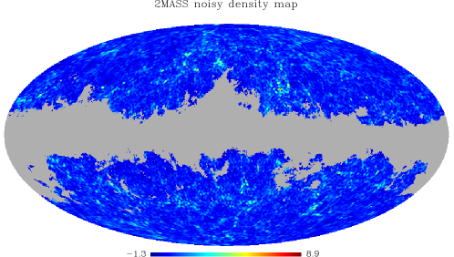
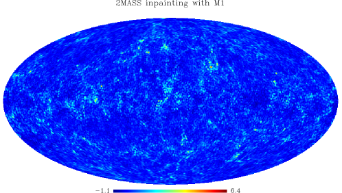
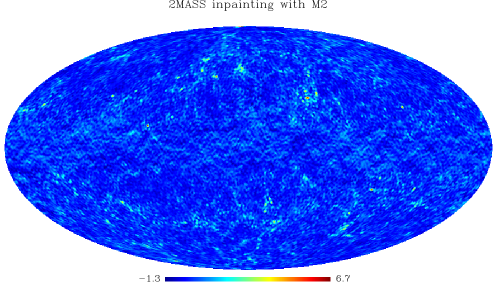
As an experiment, we apply our method on the 2MASS galaxy survey [11]. As we are working on the sphere, the dictionary $\boldsymbol{\Phi}$ contains the spherical harmonics transform, which is an orthobasis. The manually tuned parameters were $N_{\mathrm{tex}}=15$, $N_{\mathrm{est}}=40$ ,$N_{\mathrm{iter}}=6$, $N_{\mathrm{MI}}=10$, $\gamma=10^{-4}$ and $\lambda=10^{-3}$, that seems sufficient for recovering most of the large scales. This method was compared with the inpainting method proposed in [12] (denoted M2) which fills in the missing data area using both sparsity and a quadratic data fidelity.

The results are pictured by Fig. 1. In order to compare efficiently the results, we remove all the spherical harmonic modes beyond $200$ (i.e. $\ell\leqslant 200$) of the maps. Method M1 gives a better estimation of the inpainted areas, as realistic structures has been created inside these areas and the transition between missing and observed pixels are invisible. While with method M2, transitions can be clearly seen and no structure is infer inside the large missing area in the center.

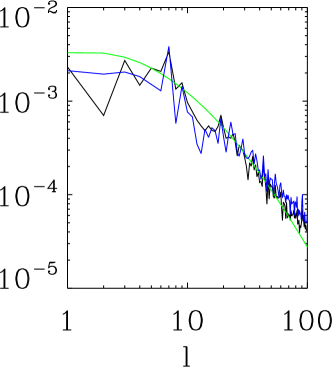
For the denoised zones, both methods preserve the structures and the amplitude. In order to compare the behavior of the two methods, we also compare in Fig. 2 the second-order statistics of the inpainted maps to the theory [13]. More precisely, we focus on the first modes of the harmonic power spectrum of the density field. While at the beginning methods M1 and M2 provide similar results, they differ on higher modes where the Poisson noise becomes more salient at the profit of the M1 method.

Fig. 1: Results on the inpainting methods on the 2MASS count map. Top: The 2MASS noisy density map with the missing data in gray. Middle and bottom: The inpainted density map using the method M1 (Middle) and M2 (bottom).

Fig. 2: The theoretical (green), M1 (black) and M2 (blue) power spectra for the first 100 harmonics modes.

4 Conclusion

An inpainting method is proposed using a data augmentation procedure, where the observation is first completed with realistic data. For galaxy density field, we propose to use two priors, first we assume that the density field follows a log-normal distribution and secondly, the underlying Gaussian field is assumed to be sparse inside a wisely chosen dictionary. The resulting algorithm is able to preserve the second order statistical properties which is an important feature for astrophysics application.

References

- [1] F. S. Kitaura, J. Jasche, C. Li, T. A. Enßlin, R. B. Metcalf, B. D. Wandelt, G. Lemson, and S. D. M. White, “Cosmic cartography of the large-scale structure with Sloan Digital Sky Survey data release 6,” MNRAS, vol. 400, pp. 183–203, Nov. 2009.
- [2] J. K. Adelman-McCarthy, M. A. Agüeros, S. S. Allam, C. Allende Prieto, et al., “The Sixth Data Release of the Sloan Digital Sky Survey,” ApJS, vol. 175, pp. 297–313, Apr. 2008.
- [3] F.-S. Kitaura, J. Jasche, and R. B. Metcalf, “Recovering the non-linear density field from the galaxy distribution with a Poisson-lognormal filter,” MNRAS, vol. 403, pp. 589–604, Apr. 2010.
- [4] P. Coles and B. Jones, “A lognormal model for the cosmological mass distribution,” MNRAS, vol. 248, pp. 1–13, Jan. 1991.
- [5] Martin A. Tanner and Wing Hung Wong, “The Calculation of Posterior Distributions by Data Augmentation,” Jour. Amer. Stat. Asso., vol. 82, no. 398, pp. 528–540, jun. 1987.
- [6] R.J.A. Little and D.B. Rubin, Statistical Analysis with Missing Data, New York: John Wiley, 1987.
- [7] J. Portilla and E. P. Simoncelli, “A Parametric Texture Model Based on Joint Statistics of Complex Wavelet Coefficients,” Int. Jour. Comp. Vis., vol. 1, no. 40, pp. 49–71, 200.
- [8] J.-J. Moreau, “Fonctions convexes duales et points proximaux dans un espace hilbertien,” CRAS Sér. A Math., vol. 255, pp. 2897–2899, 1962.
- [9] Patrick L. Combettes and Jean-Christophe Pesquet, “A proximal decomposition method for solving convex variational inverse problems,” Inverse Problems, vol. 24, no. 6, 2008.
- [10] R. Corless, G. Gonnet, D. Hare, D. Jeffrey, and D. Knuth, “On the Lambert W function,” Advances in Computational Mathematics, vol. 5, pp. 329–359, 1996, 10.1007/BF02124750.
- [11] T. Jarrett, “Large Scale Structure in the Local Universe - The 2MASS Galaxy Catalog,” Publications of the Astronomical Society of Australia, vol. 21, pp. 396–403, 2004.
- [12] P. Abrial, Y. Moudden, J.L. Starck, J. Bobin, M.J. Fadili, B. Afeyan, and M.K. Nguyen, “Morphological component analysis and inpainting on the sphere: Application in physics and astrophysics,” \jfaa, vol. 13, no. 6, 2007, 729–748.
- [13] Niayesh Afshordi, Yeong-Shang Loh, and Michael A. Strauss, “Cross-correlation of the cosmic microwave background with the 2mass galaxy survey: Signatures of dark energy, hot gas, and point sources,” Phys. Rev., vol. D69, pp. 083524, 2004.