Testing the Warm Dark Matter paradigm with large-scale structures
Abstract
We explore the impact of a WDM cosmological scenario on the clustering properties large-scale structure in the Universe. We do this by extending the halo model. The new development is that we consider two components to the mass density: one arising from mass in collapsed haloes, and the second from a smooth component of uncollapsed mass. Assuming that the nonlinear clustering of dark matter haloes can be understood, then from conservation arguments one can precisely calculate the clustering properties of the smooth component and its cross-correlation with haloes. We then explore how the three main ingredients of the halo calculations, the halo mass function, bias and density profiles are affected by WDM. We show that, relative to CDM, the halo mass function is suppressed by , for masses times the free-streaming mass-scale . Consequently, the bias of low mass haloes can be boosted by as much as for 0.25 keV WDM particles. Core densities of haloes will also be suppressed relative to the CDM case. We also examine the impact of relic thermal velocities on the density profiles, and find that these effects are constrained to scales , and hence of little importance for dark matter tests, owing to uncertainties in the baryonic physics. We use our modified halo model to calculate the non-linear matter power spectrum, and find that there is significant small-scale power in the model. However, relative to the CDM case the power is suppressed. The amount of suppression depends on the mass of the WDM particle, but can be of order 10% at for particles of mass 0.25 keV. We then calculate the expected signal and noise that our set of WDM models would give for a future weak lensing mission. We show that the models should in principle be separable at high significance. Finally, using the Fisher matrix formalism we forecast the limit on the WDM particle mass for a future full-sky weak lensing mission like Euclid or LSST. With Planck priors and using only multipoles , we find that a lower limit of should be easily achievable.
I Introduction
Within the last two decades cosmology has experienced a major observational revolution. The measurement of the Cosmic Microwave Background (CMB) anisotropies, through such surveys as COBE and WMAP, and the mapping of the large-scale structures (LSS), through galaxy redshift surveys like 2dFGRS and SDSS, have had a great impact on our knowledge of the Universe. In particular, it has led to the establishment of the ’standard model’ for cosmology: CDM model (Spergel et al., 2007) – meaning a Universe whose mass density is dominated by collisionless Cold Dark Matter (CDM) relic particles, but whose total energy density today is dominated by the constant energy of the vacuum , which is driving the current accelerated expansion of the Universe. However, fundamental questions remain unanswered: What is the true physical nature of the cold dark matter? and what is the true origin of the accelerated expansion? In this paper we focus on developing tests for the dark matter model based upon the influence that different particle candidates have upon the statistical properties of the LSSs.
There is a large body of indirect astrophysical evidence that strongly supports the CDM hypothesis (Bertone et al., 2004; Diemand and Moore, 2009; Bertone, 2010) – i.e. a heavy, cold thermal relic particle, e.g. weakly interacting massive particles, etc., that decoupled from normal matter very early in the history of the Universe. However, despite the many successes of CDM, there is also a growing body of evidence in conflict with parts of the hypothesis. Firstly, hi-resolution simulations of CDM predict several hundred dwarf galaxy halo satellites within the Local Group, whereas the observed abundance of dwarf galaxies is a factor of 10 lower (Moore et al., 1999a; Klypin et al., 1999; Peebles and Nusser, 2010; Diemand et al., 2007; Springel et al., 2008), although counting and weighing local group galaxies is not easy (Zavala et al., 2009; Macciò and Fontanot, 2010). Secondly, the inner density profiles of haloes in CDM simulations are cuspy, with the inner density falling as (Navarro et al., 1997; Moore et al., 1999b; Ghigna et al., 2000; Diemand et al., 2004; Stadel et al., 2009), whereas the density profiles inferred from galaxy rotation curves are significantly shallower (Moore et al., 1999b) (and for more recent studies see (Swaters et al., 2003; Salucci et al., 2007; de Blok et al., 2008; Gentile et al., 2009) and references there in). Thirdly the observed number of dwarf galaxies in the voids is far smaller than expected from CDM (Peebles and Nusser, 2010).
Over the past decade much work has been invested in attempting to understand these discrepancies. Some of these problems may be reconciled through more careful treatment of baryonic physics and galaxy formation. More exotic explanations for some of these problems would require modifications to gravity or scalar fields that operate only in the dark matter sector (Peebles and Nusser, 2010; Kroupa et al., 2010). Perhaps a less dramatic explanation might be the modification of the physical properties of the dark matter particle.
Over the past decade, several modifications to the CDM hypothesis have been forwarded (see for example Hogan and Dalcanton, 2000). In this work we focus on Warm Dark Matter (WDM) in a low-density dominated universe (hereafter WDM). In this scenario, the dark particle is considered to be lighter than its CDM counterpart, and retains some stochastic primordial thermal velocity, whose momentum distribution obeys Fermi-Dirac statistics (Bode et al., 2001; Boyanovsky, 2010). Two potential candidates are the gravitino (Ellis et al., 1984) and a sterile neutrino (Dodelson and Widrow, 1994), both of which require extensions of the standard model of particle physics (Bode et al., 2001; Boyarsky et al., 2009a). The main cosmological effect of WDM is that, at early times while it remains relativistic, density fluctuations are suppressed on scales of order the Hubble horizon at that time – and particles are said to free-stream out of perturbations. In fact, until matter-radiation equality, the WDM particles can also still travel a comparable distance whilst non-relativistic. Consequently, the matter power spectrum becomes suppressed on small scales. At later times the particles cool with the expansion and at the present time essentially behave like CDM – modulo any remaining primordial velocity dispersion (for more details see Dodelson and Widrow, 1994; Bode et al., 2001; Boyanovsky, 2010).
Past research on the impact of the WDM hypothesis on the phenomenology of cosmic structures has primarily focused on small-scale phenomena (Colín et al., 2000; White and Croft, 2000; Avila-Reese et al., 2001; Bullock et al., 2002; Colín et al., 2008; Zavala et al., 2009), although there are some notable studies of large-scale structures (Colombi et al., 1996; Bode et al., 2001). In short, these results show that halo abundances for masses below the free-streaming mass-scale are suppressed relative to CDM. The amount of suppression is still a point of debate: initial studies, suggested that low mass haloes might form through the fragmentation of larger perturbations, in particular along filaments (Bode et al., 2001). However, recent numerical studies (Wang and White, 2007; Polisensky and Ricotti, 2010) have cast doubt on this as a viable mechanism, since the abundance of structure forming below the free-streaming mass-scale appears to be correlated with the initial particle grid and inter-particle separation. Some simulation results have also claimed that the density profiles of WDM haloes are shallower in the inner core regions (Colín et al., 2008). Further, whilst the linear matter power spectrum is suppressed, the nonlinear one regenerates a high -tail (White and Croft, 2000).
Observational constraints suggest that sterile neutrinos can not be the dark matter: the Lyman alpha forest bounds are (Seljak et al., 2006; Boyarsky et al., 2009a), whilst those from the X-ray background are (Boyarsky et al., 2008). However a more recent assessment has suggested that a better motivated particle physics model for the production of the sterile neutrino may evade these constraints, with the new bound (Boyarsky et al., 2009b). It therefore seems that independent methods for constraining the properties of WDM from cosmology would be valuable.
In a recent paper, (Markovic et al., 2010), it was proposed that the WDM scenario could be tested through weak lensing by LSS. The advantage of such a probe is that it is only sensitive to the total mass distribution along the line of sight. However, to obtain constraints on the WDM particle mass, an accurate model for the nonlinear matter clustering is required. Markovic et al. (2010) attempted to construct this in two ways, firstly through use of the halo model and secondly through adapting a fitting formula for CDM power spectra. There appeared to be some discrepancy between the predictions of the two approaches. Furthermore, their halo model calculation suggested that the bias of high mass haloes was significantly larger than for the case of CDM. One of the aims of this paper is to construct an improved halo model calculation for application to this problem.
The paper is broken down as follows. In §II we briefly review the impact of WDM on the linear theory evolution of structure. In §III we describe our new halo model approach. In §IV we discuss the ingredients of the halo model in the context of WDM. In §V we show our results for the clustering statistics and the weak lensing observables. In §V.3 we forecast a limit on the particle mass, obtainable from a future full-sky weak lensing survey. In §VI we summarize our findings and conclude.
II Theoretical Background
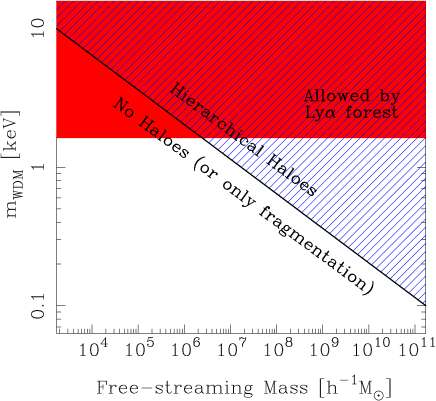
One of the major differences between structure formation in the CDM and WDM scenarios, is that whilst the dark matter particle is relativistic it free-streams through the Universe and so suppresses the growth of density perturbations on scales smaller than the free-streaming length (Bond et al., 1980; Colombi et al., 1996; Bode et al., 2001; Viel et al., 2005) 111Note that the free-streaming mass scale is not the same as the Jeans mass. In WDM the Jeans mass is set by the effective pressure of the relic thermal motions of the particles, whereas the free-streaming mass is the linear mass scale at which significant departures from a CDM model are expected. At early times when the particles are relativistic these two mass scales can coincide or are proportional. However, at late times, the Jeans length drops significantly below the free-streaming mass scale , and if the relic velocities are absent, then it is zero.. The lighter the WDM particle the longer it remains relativistic and hence the larger the free-streaming scale. Following convention, we shall define the free-streaming scale as the half-wavelength of the mode for which the linear perturbation amplitude is suppressed by a factor of 2 (Avila-Reese et al., 2001; Bode et al., 2001; Viel et al., 2005). Fitting to the solutions of integrations of the collisionless Einstein-Boltzmann equations through the epoch of recombination, sets the free-streaming scale to be (Zentner and Bullock, 2003):
| (1) |
where is the total energy density in WDM, relative to the critical density for collapse, and is the mass of the dark matter particle in keV. From the scale we may infer a putative halo mass whose formation is suppressed by the free-streaming. In the initial conditions this is given by (Avila-Reese et al., 2001):
| (2) |
In Fig. 1 we show the relation between the free-streaming mass-scale and the mass of the WDM particle candidate for our adopted cosmological model. Haloes that would have masses below the free-streaming mass-scale will have their peaks in the primordial density field erased. The impact of the free-streaming of the WDM particles on the linear growth of structure can be further described by the matter transfer function. This can be represented (Bode et al., 2001; Markovic et al., 2010),
| (3) |
where and are the linear mass power spectra in the WDM and CDM models respectively. Note that in order to avoid cumbersome notation, we shall adopt the convention , likewise for the nonlinear power spectrum in the WDM model. Fitting to results of full Einstein-Boltzmann integrations gives , and of the order (Viel et al., 2005):
| (4) |
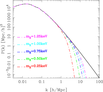
In Fig. 2 we show how variations in the mass of the WDM particles effects the linear matter power spectrum. Clearly, the lighter the WDM particle the more the power is damped on small scales.
Note that in the above we are assuming that the WDM particle is fully thermalized, i.e. the gravitino. Following (Viel et al., 2005), this can be related to the mass for the sterile neutrino through the fitting formula:
| (5) |
III Halo model approach
III.1 Statistical description of the density field
We would like to know how the nonlinear matter power spectrum changes for WDM models. In order to do this we shall adapt the halo model approach. For the case of CDM, the halo model would assume that all of the mass in the Universe is in the form of dark matter haloes and so the density field can be expressed as a sum over haloes. In WDM models this ansatz can be no longer considered true, owing to the suppression of halo formation on mass-scales smaller than . We modify this in the following way: we suppose that there is some fraction of mass in collapsed dark matter haloes and that there is a corresponding fraction in some smooth component. Hence we write the total density of matter at a given point as:
| (6) |
where is the density in smooth matter, and is the mass normalized isotropic density profile, and both depend on the mass of the WDM particle – for convenience we suppress this label. The sum in the above extends over all haloes and subhaloes. The mean mass density of the Universe can be written,
| (7) |
where the expected total mass density in WDM haloes and the smooth component can be written,
| (8) |
where is the mean density of all matter, and the fraction of mass in haloes. This can be written,
| (9) |
where is the number density of WDM haloes per unit mass and is the mass-scale below which there are no haloes. In this study we will take , but will formally make the distinction throughout.
Let us now work out the clustering statistics in this model. The two point correlation function of the mass density can be written:
| (10) | |||||
Owing to the statistical homogeneity and isotropy, we have that . The correlation function between two random density fields X and Y can be written:
| (11) |
where the dimensionless over-density field is defined:
| (12) |
On using the above definition, we find that
| (13) |
Thus the correlation function is simply the weighted average of the smooth-mass correlation function , the mass weighted halo-halo correlation functions and the smooth mass-halo cross correlation function . In order to proceed further, we need to understand these three correlation functions.
III.2 Halo-halo correlation function
Let us first consider the halo-halo correlation function, this can be derived following (Cooray and Sheth, 2002, and references therein). The clustering is the sum of two terms: the 1-Halo term, which describes the clustering of points within the same halo and the 2-Halo term, which correlates the mass distribution between haloes. Thus we have,
| (14) |
where these terms have the explicit forms (Cooray and Sheth, 2002):
| (15) | |||||
| (16) | |||||
where in Eq. (16) and denote the position vectors of the center of mass of halo 1 and 2, and and denote position vectors of the points to be correlated, respectively. Thus gives the radial vector from the center of halo 1 to the point 1, and likewise for halo 2. Further, owing to the statistical isotropy of the clustering .
In principle the correlation function of halo centers (with ), is a complicated scale dependent function of , and (e.g. see Smith et al., 2007). We assume that there is a local deterministic bias relation between haloes and dark mass, smoothed on a scale . Hence, we have (Fry and Gaztanaga, 1993; Mo and White, 1996; Smith et al., 2007):
| (17) |
where the are the nonlinear bias parameters. Thus the halo center correlation function has the form:
| (18) | |||||
where is the nonlinear matter correlation function smoothed on scale . On truncating the above expression at first order in and inserting into Eq. (16), one finds:
| (19) | |||||
Before moving on, we note that in practice, in order to make accurate predictions in the halo model on small scales, we must take into account halo exclusion (Takada and Jain, 2004; Smith et al., 2007, 2010). That is, the separation of two distinct haloes can not be smaller than the sum of their virial radii. Otherwise, they would have been identified as a larger halo. However, when modelling WDM there is a new “exclusion” condition that arises, the smooth component is not really smooth. Formally there are holes of zero density in the smooth distribution where haloes are. Since these calculations are first order attempts, we shall leave such detailed analysis for future study.
III.3 Smooth-smooth correlation function
Let us next consider the smooth mass component of the model. We shall assume that this represents all of the mass that was initially in mass peaks of the density field that were . In direct analogy with the density field of dark matter haloes, we may assume that the smooth component can be related to the total mass density field through a deterministic local mapping. Hence,
| (20) |
where the are the nonlinear bias parameters of the smooth component. This leads us to write an expression similar to Eq. (18),
| (21) |
III.4 Halo-smooth mass cross-correlation
The model also requires us to specify the cross-correlation between the mass in haloes and the mass in the smooth component. This can be written in the following fashion,
| (22) | |||||
where .
III.5 Power spectrum
The correlation functions are related to the matter power spectra through a Fourier transform (Peebles, 1980; Peacock, 1999; Cooray and Sheth, 2002):
| (23) |
On applying this to Eqns (14), (21), and (22), one finds
| (24) |
where the power spectra of the smooth-smooth, smooth-halo and halo-halo components, can be written to first order in the halo and smooth density bias parameters as,
| (25) | |||||
| (26) | |||||
| (27) | |||||
where is the nonlinear mass power spectrum smoothed on a scale , and is the Fourier transformed mass normalized density profile, .
III.6 Bias of the smooth component
Absent so far is any explanation as to how one might infer the bias factors of the smooth component . We shall now use a mass conservation argument to derive a relation between the bias of the smooth mass and the bias of the haloes that involves no new free parameters. That is, if we fully understand halo biasing, then we may immediately obtain a full understanding of the density distribution of the smooth density component.
Consider again the density at a given point, this may be written as in Eq. (6), i.e. . On using Eqns (7), (8) and (12), then we may write this in terms of the overdensities in the smooth and clumped matter as
| (28) |
The mass density associated with matter in haloes can be written as an integral over all haloes above the mass-scale in the following manner,
| (29) | |||||
If we assume the local model for halo biasing of Eq. (17), then the density field of haloes takes the form:
| (30) |
where . Next, let us define the effective mass weighted halo bias parameters as,
| (31) |
Then we may re-write Eq. (30) more simply as
| (32) |
Substituting the above equation and the local bias model from Eq. (20) into Eq. (28), we then find
| (33) | |||||
On inspecting the above equation, two conditions may be immediately noticed. Firstly, in order for the left and right sides of the equation to balance, we must have that
| (34) |
This leads us to the result that the bias of the smooth component must be given by,
| (35) |
Secondly, if the smooth component is indeed linearly biased with respect to the total matter overdensity, then we must also have that the nonlinear bias coefficients vanish when integrated over all haloes:
| (36) |
On the other hand, supposing that the smooth component is not simply linearly biased, but is nonlinearly biased a la the local model, then the above condition is relaxed to the condition:
| (37) |
This leads us to the condition,
| (38) |
Hence, if the haloes and the smooth mass component are locally biased, then all of the nonlinear bias parameters for the smooth component can be derived from knowledge of the halo bias parameters. In §IV.2 we will show how the bias of the smooth component varies for different mass-scales of the WDM particle.


IV Halo Model ingredients in WDM models
In this section we detail the halo model ingredients and show how they change in the presence of our benchmark set of WDM particle masses.
IV.1 Halo mass function
In order to predict the abundance of haloes in the WDM cosmological model, we shall adopt the Press-Schechter (PS) (Press and Schechter, 1974) approach, with some small modification. For mass-scales , we shall assume that the standard formalism holds. In this case we may calculate the abundance of objects through the usual recipe, only being sure to use the appropriate linear theory power spectrum for WDM. Hence,
| (39) |
where is the abundance of WDM haloes of mass in the interval , is the linear theory collapse barrier for the spherical collapse model, and is the linear theory growth function. Note that we take the evolution of and to be unchanged from their forms in the CDM model. Our reasoning is that, if one follows the standard derivations for and , then, provided the WDM particles decouple early and are non-relativistic today, these functions are solely determined from the dynamics of the expansion rate of the Universe. This assumption will of course break down at very early times, when the primordial thermal velocities are more significant and when the particles are relativistic and so growth suppressed.
For the function we adopt the model of Sheth and Tormen (1999), and this has the form:
| (40) |
For the ST mass function the amplitude parameter is determined from the constraint , which leads to . The parameters are: . The variance on mass-scale and its derivative with respect to the mass scale can be computed from the following integrals:
| (41) | |||||
| (42) |
where the filter functions are and . For a 3D real-space spherical top-hat filter, transformed into Fourier space, we have:
| (43) | |||||
| (44) |
For mass-scales , free-streaming erases all peaks in the initial density field, and hence peak theory should tell us that there are no haloes below this mass scale. A blind application of the PS approach leads one to predict, suppressed, but significant numbers of haloes below the cut-off mass.
In order to demonstrate this point explicitly, let us consider the following toy-model calculation. Suppose that the matter power spectrum is a simple power-law , and let us suppose that if the dark matter particle is warm then the effect of the damping on the fluctuations due to free-streaming can be represented by a simple exponential damping. Hence, , where is a characteristic damping scale; perhaps . Let us now consider the behaviour of Eqs (41) and (42) in the limit that . For the variance term we have:
| (45) | |||||
where we have used the fact that . For the derivative of the variance we have:
| (46) | |||||
where we used the fact that . Thus as (or equivalently ), the mass function of dark matter haloes becomes:
| (47) | |||||
where in the above we have defined
| (48) |
Hence, we see that the number density of haloes per logarithmic interval diverges, , but that the multiplicity function of haloes asymptotes to a constant value, .
We show this behaviour more schematically in the left panel of Fig. 3 (dot-dashed curves), where we compare CDM and WDM mass functions. For large halo masses , the models are virtually indistinguishable, even for the case of a WDM particle with mass . However, for smaller halo masses, whilst there is a significant suppression, they are still highly abundant.
Recent results from numerical simulations show that there is a strong suppression in the numbers of haloes with (Zavala et al., 2009; Polisensky and Ricotti, 2010). Also, there is some debate as to whether haloes below the cut-off can form at all (Bode et al., 2001; Wang and White, 2007). We shall take the view that PS is correct for , but that below this mass one finds virtually no haloes. We model this transition in an ad-hoc manner using an error function as a smoothed step. Thus the mass function in WDM becomes:
| (49) |
where controls the logarithmic width of the step, and controls the location of the step. In this work, for simplicity we shall take , and so the function acts like a standard Heaviside function at . We show the results of this modification in Fig. 3 (solid lines). For this example we have chosen .
The exact amount of suppression in the WDM mass functions, relative to CDM, can be better quantified through inspecting the right panel of Fig. 3. Here we show the fractional difference between the WDM and CDM models versus halo mass-scaled in units of . The plot shows that there is roughly a suppression in the abundance of haloes with in all of the WDM models considered.
IV.2 Halo bias
The halo model also requires us to specify how the centers of dark matter haloes of different masses cluster with respect to each other. As described by Eq. (18), for the Gaussian model, and at first order in the dark matter density, halo and matter density perturbations can be related through a scale-independent bias factor . Following (Mo and White, 1996; Sheth and Tormen, 1999), an application of the peak-background split approximation enables one to calculate from a given mass function. For the ST mass function the Gaussian bias has the form:
| (50) |
where the parameters are as in Eq. (40).
For the case of WDM, we shall assume that for haloes with the bias is well described by the same peak-background split model. Hence in model space: .
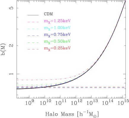
In the left panel of Fig. 4 we show how the bias of dark matter haloes in both CDM and WDM models depends on the halo mass. The figure shows the results for the set of WDM particle masses: . As for the mass function, for high mass haloes with , the bias is virtually indistinguishable from that obtained for CDM. For the case of lower masses, we see that the bias has a clear dependence on the mass of the WDM particle. For lower mass particles the bias of low mass haloes is significantly boosted with respect to CDM.
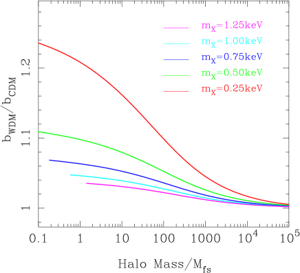
The right panel of Fig. 4 shows this last point in more detail. Here we plot the ratio of the bias in the WDM model with respect to that of the CDM model, and we scale the halo mass in terms of the free-streaming mass-scale . We now see that there is roughly a boost in the bias for haloes with and with a WDM particle mass .
The left panel of Fig. 4 also shows how the bias of the smooth mass distribution varies with respect to . This was calculated using Eq. (35), and assuming the ST mass function and bias parameter from above. We find that the smooth component is anti-biased with respect to the total matter, with for the cases , respectively. Note that as the particle mass increases the bias of the smooth component saturates. This arises due to the fact that, for , and hence from Eq. (50),
| (51) | |||||
IV.3 Halo density profiles
The density profiles of CDM haloes have been studied in great detail over the last two decades. A reasonably good approximation for the spherically averaged density profile in simulations is the NFW model Navarro et al. (1997):
| (52) |
where the two parameters are the scale radius and the characteristic density . If the halo mass is , then owing to mass conservation there is only one free parameter, the concentration parameter . Hence,
| (53) |
The concentration parameter can be obtained from the original model of NFW, but we shall instead use the model of Bullock et al. (2001). Note that for our halo model calculations we shall correct for the fact that the definitions of the virial mass in Bullock et al. and Sheth & Tormen are different (Smith and Watts, 2005).
In the case of the WDM model, there are two major effects which modify the density profiles when compared to CDM. Firstly, if one adopts either the NFW (Navarro et al., 1997) or Bullock et al. (Bullock et al., 2001) approach for calculating the concentration parameters, then one finds, owing to the suppression of small-scale power, that the collapse redshifts of the haloes are significantly affected. Thus a given halo of mass in the WDM model, will be expected to collapse at a later time than in the CDM model. Since halo core density is related to the density of the Universe at the collapse time, then one expects that core densities in WDM models will be suppressed, and haloes on average to be less concentrated.
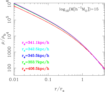
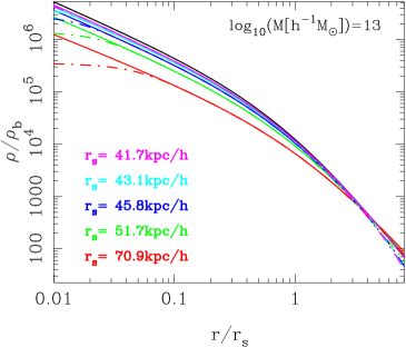
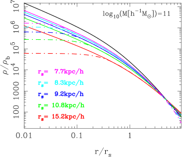
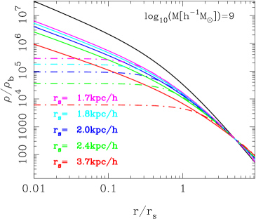
We explicitly demonstrate this point in Fig. 5. The top left, top right, bottom left, and bottom right panels show density profiles for haloes of mass , respectively. The CDM case is shown as the black solid line, and the case where the mass of the dark matter particle is decreased, is shown as the series of curves with decreasing amplitude. Clearly, smaller mass haloes are more significantly affected by the absence of small-scale power. However, we do note that higher mass haloes are not immune to this, there being signs of density suppression in haloes with for .
Secondly, it has been argued, owing to the preservation of Liouville’s theorem and the existence of a relic thermal velocity distribution for the dark matter particles, that there is a fundamental limit on the size of core densities in phase space (Tremaine and Gunn, 1979; Colín et al., 2008). If this is correct, then cuspy density profiles are prohibited in the WDM model. In order to mimic the effect of the phase space constraint on the profiles, we take a qualitative approach and simply convolve the NFW profile (obtained from computing collapse times with the WDM power spectrum) with a Gaussian filter function of radius the mean thermal velocity scale of the WDM particles.
This can be calculated as follows: Let us suppose that the WDM particles are leptons and so obey the Fermi-Dirac (FD) statistics. Also, we assume that the gas decoupled from the rest of matter whilst still relativistic, i.e. the energy of a given particle is . Thus its phase space distribution remains unchanged, except cooling adiabatically through the expansion of the Universe. Hence, the FD distribution function can be written:
| (54) |
Fitting to the results from the evolution of Einstein-Boltzmann codes gives the characteristic velocity (temperature) to be (Bode et al., 2001):
| (55) | |||||
where is the number of degrees of freedom per particle, and we take this to be similar to that of a light neutrino species, hence (Bode et al., 2001). Next, in order to calculate statistics, we also require the density of momentum states, for a quantum gas this is: . Hence, the mean and rms velocities can now be calculated:
| (56) | |||||
| (57) |
In order to obtain the last equalities in both Eqs (56) and (57), we have used the normalization condition,
| (58) |
and are Riemann Zeta functions. Evaluation of Eqs (56) and (57) gives: and . Table 1 presents the velocity statistics for our fiducial set of WDM particle masses.
| 0.25 | 0.065 | 0.204 | 0.234 | 2.04 |
| 0.50 | 0.026 | 0.082 | 0.094 | 0.82 |
| 0.75 | 0.015 | 0.047 | 0.054 | 0.47 |
| 1.00 | 0.010 | 0.032 | 0.036 | 0.32 |
| 1.25 | 0.008 | 0.025 | 0.029 | 0.25 |
Finally, the density profile smoothed on the scale of the mean relic velocity field, is given by
| (59) |
where , and where is the mass normalized profile. We truncate the CDM profile at the virial radius and for the NFW model the Fourier transform can be written as (Cooray and Sheth, 2002):
| (60) | |||||
where and where and are the standard sine and cosine integrals.
In Fig. 5 we show the impact of relic velocities on the density profiles. If the relic velocities are present and act to simply smooth the density field, then, by fiat, we see that halo cusps are suppressed. Importantly, the figure shows, for the range of WDM particle masses considered, that only haloes with show any noticeable effects due to the relic velocities on scales .
V Results

V.1 Mass power spectra
In Fig. 6 we compare the WDM and CDM nonlinear matter power spectra obtained from the halo model calculations. The figure shows the contribution of each of the halo model terms to the WDM spectrum. For the purposes of clarity we show this for one case only, a WDM particle with . This is instructive, as it shows that on large scales the power is totally determined by the weighted contributions , and . However, on small scales the power is entirely dominated by the haloes that exist above the free-streaming mass-scale. The integrand of the 1-Halo term is . Since there are virtually no differences between the mass function in WDM and CDM for haloes above , the apparent suppression in power comes entirely from the suppression in the abundance of small haloes and the change in the profiles.
In Fig. 6 we also show the importance of the relic velocities on the matter power spectrum. As can clearly be seen, at present times the halo model power spectra with and without the relic velocity effects are indistinguishable for scales . On these scales, the modifications to the power spectrum due to uncertainties in the baryonic physics are significantly more important. We therefore assume that the present day effects of relic velocities will be unimportant for constraining the WDM particle from large-scale structure probes.
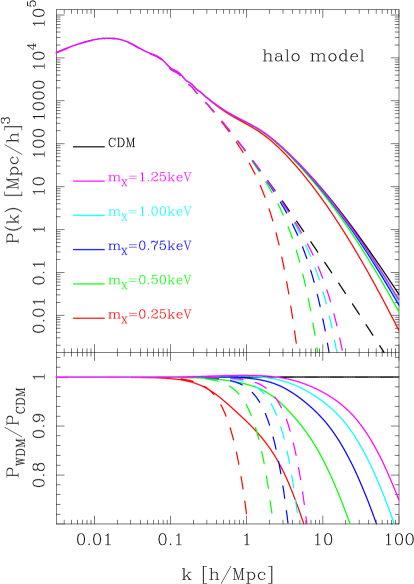
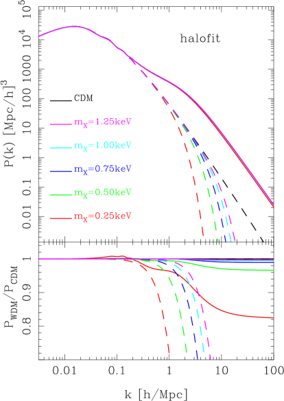
In the left panel of Fig. 7, we show the dependence of the nonlinear matter power spectra on the WDM particle mass. We see that, whilst the linear theory power spectra are significantly damped, the nonlinear halo model predictions show that a large amount of small scale power is generated. As noted above this arises due to the collapse of haloes above the free-streaming mass-scale. The bottom panel of Fig. 7 allows us to quantify the differences in greater detail. Here we show the ratio of the linear WDM and CDM spectra, and also the ratio of the nonlinear WDM and CDM spectra. From this we understand that the relative difference in the nonlinear model is significantly less than the difference between the linear theory predictions. For our cosmological model, the effect of going from the CDM model to WDM model with particle mass , is to cause a suppression of power at .
In the right panel of Fig. 7, we show the nonlinear predictions for the WDM power spectra from the halofit code of (Smith et al., 2003). This semi-empirical method was designed to match CDM power spectra. It is not clear whether this method can be accurately extrapolated to model nonlinear WDM spectra. Comparing the left and right panels of the figure, we see that the halo model predicts a stronger suppression of nonlinear power than halofit, and also a greater difference between the predictions for each WDM particle. It will require hi-resolution -body simulations, to disentangle which of these two models provides the better description for the power spectrum in WDM models.
At this juncture, one might question the validity of the halo model predictions given our assumptions concerning the cut-off mass scale and also our adoption of the NFW profile for these same haloes. In Appendix A.1 and A.2, we show that the predictions for the power spectrum are insensitive to the precise value of (no changes are found over two-orders of magnitude in mass around ), and the exact shape of the profiles of these objects. More quantitatively, the predictions are modified by for scales and for WDM particle masses .
V.2 Weak lensing convergence power spectra
We now turn to the question: Can the modifications to the dark matter model, of the kind considered in this paper, be detected with next generation surveys? To answer this, we shall focus on weak gravitational lensing by cosmic LSS as the most direct observable.
Weak lensing is the magnification and shearing of light rays from distant source galaxies as they propagate through the inhomogeneous matter in the Universe on their way towards the observer. Owing to our ignorance of the intrinsic shapes of the unlensed galaxies, these distortions can only be measured through the correlations in the shapes of the source galaxies with each other. Following (Bartelmann and Schneider, 2001), the weak lensing angular power spectrum of convergence is given by
| (61) |
where is the comoving geodesic distance from the observer to redshift , and is the comoving angular diameter distance to redshift . The survey weight function is defined:
| (62) |
The function is the normalized source distance distribution function, which tells us the number of sources per unit distance interval . For simplicity we shall assume the source distribution is a Dirac delta function at a single source plane, hence . In this case the survey weights simplify to and we have,
| (63) |
Direct numerical integration of the above expression can be very slow, since it requires the evaluation of the halo model integrals for many points in the plane, for a given . The most efficient way to overcome this problem, is to generate a bi-cubic spline (Press et al., 1992) fit to evaluated on a cubical grid of and . We found a mesh of size gave good results, with and . Once the bicubic spline is generated, the evaluation of the halo model takes of order the same time to compute as the linear calculation.
We now make a rough assessment of the expected errors on the convergence power spectrum for a future weak lensing survey. To do this, we assume that the spherical harmonic multipole coefficients are independent Gaussianly distributed variables. In this case the covariance matrix for a measurement of the power spectrum in band powers and can be written (Takada and Jain, 2004):
| (64) |
where is the fraction of sky covered, is the angular number density of galaxies on the sky, is the shape noise error, which is the error on a given measurement of the ellipticity of a galaxy. is the number of independent multipoles used to generate the estimate of in a given band power. For a given band power , we find that
| (65) |
For our fiducial survey we assume future full-sky weak lensing mission, like the proposed Euclid (Refregier et al., 2010) or LSST (LSST, 2009) surveys: , galaxies per square arc minute, and we take 50 bins in log- in the range .
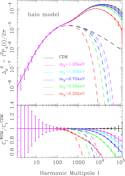
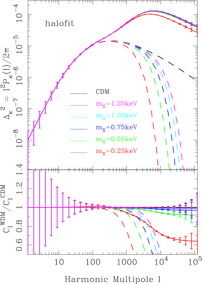
The left panel of Fig. 8 shows the convergence matter power spectrum for the linear and nonlinear halo model predictions for both CDM and the WDM models. For large angular scales, , the linear and nonlinear predictions agree and there is no difference between CDM and WDM. However, on smaller scales we see significant departures between the predicted spectra. The importance of the nonlinear corrections is very apparent: by , there is an order of magnitude difference between the linear and nonlinear predictions, and by , the difference is more than two orders of magnitude for the WDM models. As expected, we also see that the measurement errors are largest on very large and small scales, due to cosmic variance and shape noise, respectively.
The bottom panel of Fig. 8 shows the relative differences between the WDM and CDM models. We see clearly that nonlinear evolution reduces the differences between the WDM models and CDM. However, the error bars show that the WDM models and the CDM should be distinguishable at high significance.
The right-hand panel of Fig. 8 shows the same but for the case where the nonlinear power is computed using halofit. The main differences are: for the predictions from both methods are roughly comparable, but for the halo model has at least a factor 2 less signal than that obtained from halofit. The implications of this are that if the halofit is correct and the halo model is wrong, then this will diminish the ability of future weak lensing surveys to constrain the mass of the WDM particle. Nevertheless, as was shown recently in (Markovic et al., 2010), reasonably good constraints may still be achievable.
Note that for these ‘signal-to-noise’ predictions, we have assumed that all of the source galaxies lie at . In the next section we perform a more complete Fisher matrix analysis with a full redshift distribution.
V.3 Fisher matrix forecast for
Finally, we make a forecast for the lower limit on obtainable with our fiducial (Euclid-like/LSST-like) survey. Owing to these future missions including extensive photometric and spectroscopic redshift survey components, we now take advantage of this expected knowledge and assess the performance of a tomographic lensing analysis (see for example Hu, 1999; Takada and Jain, 2004).
We adapt the analysis of the previous section as follows. We assume an extended source redshift distribution for in Eq. (62), and for this we take the same form as in (Markovic et al., 2010). We then divide the distribution into 10 separate tomographic redshift bins. The lensing convergence power spectrum from the cross-correlation of sources in bins and is then given by:
| (66) |
where the weight function has the form:
| (67) |
and where and is the source redshift distribution. Assuming that the underlying density field obeys Gaussian statistics, then it can be shown that measurements of the convergence power spectra for different tomographic bins are correlated provided they share the same spherical harmonic multipole . In this case the covariance matrix can be written (Takada and Jain, 2004):
| (68) |
where we defined . In the above expression we have again ignored contributions to the covariance from higher order spectra (Smith, 2009).
Assuming that the likelihood function for obtaining measurements of the convergence power spectrum in several band powers and for several tomographic bins is well described by a multivariate Gaussian distribution with covariance matrix as given by Eq. (68), then the Fisher matrix can be written (Takada and Jain, 2004):
| (69) |
where and are elements of the vector of cosmological model parameters upon which our measurements depend. and label the distinct pairs of tomographic bins, i.e. . The marginalized variance and covariances of the cosmological parameters can be obtained in the usual way (for further details see Heavens, 2009): and .
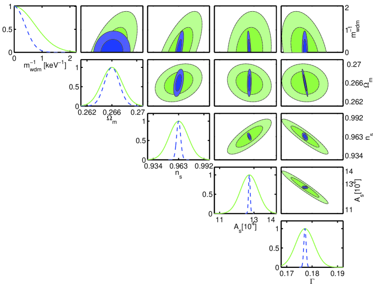
For our lensing analysis we choose to vary five parameters : the inverse WDM particle mass; the total matter density today; the primordial perturbation spectral index; the primordial spectral amplitude; and the matter power spectrum shape parameter, . Note that, since our fiducial model is CDM with fiducial parameters given by the WMAP7 data (Komatsu et al., 2010), we choose to work with as a parameter in order to avoid setting the fiducial model parameter to infinity. However, redefining this variable does not avoid the strong variation of the error on with the chosen fiducial model. Furthermore, and most problematically for such an analysis, the likelihood function is flat with respect to the variation of this parameter around the maximum likelihood point. For this reason we fit half a Gaussian curve on top of this likelihood function and find single tailed errors as described in Markovic et al. (2010).
Figure 9 presents the 1- and 2-D likelihood contours centered on our fiducial model. For the 2-D likelihood contours the 1- and 2- contours are denoted by the light and dark green shaded regions, respectively.
We then combine our lensing forecast with Planck (The Planck Collaboration, 2006) priors, i.e . We use the Planck Fisher matrix for the fiducial parameter set prescribed by (Albrecht et al., 2006). We marginalize over the optical depth and the baryon density and perform a parameter transformation as in (Eisenstein et al., 1999; Rassat et al., 2008). As in (Markovic et al., 2010), we assume that we will only have the 143 GHz channel for CMB data. Furthermore, we assume that WDM with particle masses of the order of a keV, does not leave an observable signature in the CMB and hence set the corresponding entries in the Planck Fisher matrix to zero. The result of adding the Planck priors can be seen in the Fig. 9 as the blue contours and lines.
Finally our forecast for the minimum limit on the WDM particle mass, assuming that the CDM scenario is correct, from a Euclid/LSST-like survey is . On combining our fiducial lensing survey and Planck data, the constraint tightens to . We note that this limit is comparable to that found in (Markovic et al., 2010). However, our analysis is more conservative since we consider only multipoles , compared to used in the study by (Markovic et al., 2010). Moreover, at the median redshift of the Euclid survey, , corresponds to approximately . The main reasons for excluding small scales from the analysis are: one, to avoid the range of scales where unknown baryonic physics effects inside clusters may be a significant source of bias for interpreting the data (Zhan and Knox, 2004); two, the assumption of a decorrelated covariance matrix for different ’s breaks down due to nonlinear mode coupling in the density field, resulting in a loss of information Scoccimarro et al. (2001); Sato et al. (2010).
VI Conclusions
In this paper we have explored a new approach to modelling the nonlinear evolution of two-point mass clustering statistics in the WDM scenario. The model is based on the phenomenological halo model approach.
In §II we gave a brief overview of how linear structure formation is changed in the WDM scenario. We defined a free-streaming mass-scale , below which halo formation is likely to be strongly suppressed.
In §III we developed the halo model of large-scale structure. We extended the model by including two components of clustered mass in the Universe. That which is in collapsed dark matter haloes and that which is in the form of smooth uncollapsed mass. This extended model requires that we understand three correlation functions: the halo-halo, smooth-halo and smooth-smooth correlation functions. The halo-halo clustering can be calculated as in the standard halo model. The clustering of the smooth matter is biased with respect to the total mass. We showed that, provided one understands the halo-halo correlation function, then the bias of the smooth component can be derived from simple conservation arguments.
In §IV we explored how the standard halo model ingredients, i.e. halo mass function, halo bias and density profiles are modified in the context of the WDM model. We showed that an application of the standard mass function theory, using the WDM power spectrum, leads to a 50% suppression in halo abundance relative to CDM for mass-scales . For our halo model calculations we assumed that no haloes formed below .
For the halo bias, we assumed that the standard peak-background split calculations applied equally to the WDM model. Under this assumption, we showed that the bias of haloes with can be larger by for WDM models than CDM ones, for . Otherwise, halo bias is not affected. We also computed the bias for the smooth component and found that it was anti-biased with respect to the total mass, typically with a bias of order , for the range of WDM particle masses that we considered.
In modelling the impact of WDM on the density profiles, we took into account two effects: firstly, the change in core density and concentration due to the lower formation redshift in WDM models; secondly, the suppression of density cusps due to relic thermal velocities of the WDM particles. We found that the former effect is the most important. Relic velocities only affect the density structure on scales , these are irrelevant for weak lensing analysis and so can be neglected.
In §V we computed the nonlinear matter power spectrum in the halo model and showed that, whilst the linear power is strongly suppressed on small scales, nonlinear evolution generates significant small-scale power. Relative to CDM the nonlinear WDM spectra are suppressed by 10% on scales for a WDM particle with mass . For a heavier WDM particle the suppression is much less, for the suppression is only on scales . We compared the predictions from the halo model with those from the halofit prescription (Smith et al., 2003). We found that the latter showed more small scale power, but that the differences between results for different WDM particle masses was not as apparent as in the case for the Halo Model. It will require high resolution -body simulations to validate which of the two models is more realistic.
We then computed the impact of a set of WDM particle masses on the expected convergence power spectrum from a future weak lensing survey. We also calculated the expected errors, assuming that each spherical harmonic is an independent Gaussian variable. We found that, if our halo model is correct, then it would be possible to differentiate between different WDM candidates with a systematics free, full-sky, weak lensing survey like Euclid (Refregier et al., 2010) or LSST (LSST, 2009).
Finally, using the Fisher matrix approach we then forecasted the lower limit on the WDM particle mass that would obtain from a Euclid like weak-lensing mission. We made the conservative assumption that multipoles can only be safely interpreted, and we found the lower limit for Euclid only. On combining this with a forecast of the Planck CMB data, the constraint tightened to . Our findings are in agreement with the earlier study of Markovic et al. (2010), however these earlier results were obtained assuming the less conservative multipole range .
CDM and WDM are equally plausible candidates for dark matter. We should therefore invest resources in to future cosmological experiments that allow us to place constraints on the mass of the dark particle. We expect that a full-sky weak lensing survey combined with the Planck data will greatly help achieve this objective.
Acknowledgements
We thank Darren Reed for comments on an earlier draft, and an anonymous referee for helpful suggestions. We thank Gianfranco Bertone, Sarah Bridle, Alan Heavens, Martin Kilbinger, Ben Moore, Aurel Schneider and Jochen Weller for useful discussions. RES acknowledges support from a Marie Curie Reintegration Grant, an award for Experienced Researchers from the Alexander von Humboldt Foundation and partial support from the Swiss National Foundation under contract 200021-116696/1. KM acknowledges support from the International Max-Planck Research School.
References
- Spergel et al. (2007) D. N. Spergel, R. Bean, O. Doré, M. R. Nolta, C. L. Bennett, J. Dunkley, G. Hinshaw, N. Jarosik, E. Komatsu, L. Page, et al., ApJS 170, 377 (2007), eprint arXiv:astro-ph/0603449.
- Bertone et al. (2004) G. Bertone, D. Hooper, and J. Silk, Phys. Rep. 405, 279 (2004).
- Diemand and Moore (2009) J. Diemand and B. Moore, ArXiv e-prints (2009), eprint 0906.4340.
- Bertone (2010) G. Bertone, ed., Particle Dark Matter: Observations, Models and Searches (Cambridge University Press, Cambridge, UK, 2010).
- Moore et al. (1999a) B. Moore, S. Ghigna, F. Governato, G. Lake, T. Quinn, J. Stadel, and P. Tozzi, ApJL 524, L19 (1999a), eprint arXiv:astro-ph/9907411.
- Klypin et al. (1999) A. Klypin, A. V. Kravtsov, O. Valenzuela, and F. Prada, ApJ 522, 82 (1999), eprint arXiv:astro-ph/9901240.
- Peebles and Nusser (2010) P. J. E. Peebles and A. Nusser, Nature 465, 565 (2010), eprint 1001.1484.
- Diemand et al. (2007) J. Diemand, M. Kuhlen, and P. Madau, ApJ 667, 859 (2007), eprint arXiv:astro-ph/0703337.
- Springel et al. (2008) V. Springel, J. Wang, M. Vogelsberger, A. Ludlow, A. Jenkins, A. Helmi, J. F. Navarro, C. S. Frenk, and S. D. M. White, MNRAS 391, 1685 (2008), eprint 0809.0898.
- Zavala et al. (2009) J. Zavala, Y. P. Jing, A. Faltenbacher, G. Yepes, Y. Hoffman, S. Gottlöber, and B. Catinella, ApJ 700, 1779 (2009), eprint 0906.0585.
- Macciò and Fontanot (2010) A. V. Macciò and F. Fontanot, MNRAS 404, L16 (2010), eprint 0910.2460.
- Navarro et al. (1997) J. F. Navarro, C. S. Frenk, and S. D. M. White, ApJ 490, 493 (1997), eprint arXiv:astro-ph/9611107.
- Moore et al. (1999b) B. Moore, T. Quinn, F. Governato, J. Stadel, and G. Lake, MNRAS 310, 1147 (1999b), eprint arXiv:astro-ph/9903164.
- Ghigna et al. (2000) S. Ghigna, B. Moore, F. Governato, G. Lake, T. Quinn, and J. Stadel, ApJ 544, 616 (2000), eprint arXiv:astro-ph/9910166.
- Diemand et al. (2004) J. Diemand, B. Moore, and J. Stadel, MNRAS 353, 624 (2004), eprint arXiv:astro-ph/0402267.
- Stadel et al. (2009) J. Stadel, D. Potter, B. Moore, J. Diemand, P. Madau, M. Zemp, M. Kuhlen, and V. Quilis, MNRAS 398, L21 (2009), eprint 0808.2981.
- Swaters et al. (2003) R. A. Swaters, B. F. Madore, F. C. van den Bosch, and M. Balcells, ApJ 583, 732 (2003), eprint arXiv:astro-ph/0210152.
- Salucci et al. (2007) P. Salucci, A. Lapi, C. Tonini, G. Gentile, I. Yegorova, and U. Klein, MNRAS 378, 41 (2007), eprint arXiv:astro-ph/0703115.
- de Blok et al. (2008) W. J. G. de Blok, F. Walter, E. Brinks, C. Trachternach, S.-H. Oh, and R. C. Kennicutt, Jr., Astronomical Journal 136, 2648 (2008), eprint 0810.2100.
- Gentile et al. (2009) G. Gentile, B. Famaey, H. Zhao, and P. Salucci, Nature 461, 627 (2009), eprint 0909.5203.
- Kroupa et al. (2010) P. Kroupa, B. Famaey, K. S. de Boer, J. Dabringhausen, M. S. Pawlowski, C. M. Boily, H. Jerjen, D. Forbes, G. Hensler, and M. Metz, A&A 523, A32+ (2010), eprint 1006.1647.
- Hogan and Dalcanton (2000) C. J. Hogan and J. J. Dalcanton, PRD 62, 063511 (2000), eprint arXiv:astro-ph/0002330.
- Bode et al. (2001) P. Bode, J. P. Ostriker, and N. Turok, ApJ 556, 93 (2001), eprint arXiv:astro-ph/0010389.
- Boyanovsky (2010) D. Boyanovsky, ArXiv e-prints (2010), eprint 1011.2217.
- Ellis et al. (1984) J. Ellis, J. S. Hagelin, D. V. Nanopoulos, K. Olive, and M. Srednicki, Nuclear Physics B 238, 453 (1984).
- Dodelson and Widrow (1994) S. Dodelson and L. M. Widrow, Physical Review Letters 72, 17 (1994), eprint arXiv:hep-ph/9303287.
- Boyarsky et al. (2009a) A. Boyarsky, J. Lesgourgues, O. Ruchayskiy, and M. Viel, Journal of Cosmology and Astro-Particle Physics 5, 12 (2009a), eprint 0812.0010.
- Colín et al. (2000) P. Colín, V. Avila-Reese, and O. Valenzuela, ApJ 542, 622 (2000), eprint arXiv:astro-ph/0004115.
- White and Croft (2000) M. White and R. A. C. Croft, ApJ 539, 497 (2000), eprint arXiv:astro-ph/0001247.
- Avila-Reese et al. (2001) V. Avila-Reese, P. Colín, O. Valenzuela, E. D’Onghia, and C. Firmani, ApJ 559, 516 (2001), eprint arXiv:astro-ph/0010525.
- Bullock et al. (2002) J. S. Bullock, a. A. V. Kravtsov, and P. Colín, ApJL 564, L1 (2002), eprint arXiv:astro-ph/0109432.
- Colín et al. (2008) P. Colín, O. Valenzuela, and V. Avila-Reese, ApJ 673, 203 (2008), eprint 0709.4027.
- Colombi et al. (1996) S. Colombi, S. Dodelson, and L. M. Widrow, ApJ 458, 1 (1996), eprint arXiv:astro-ph/9505029.
- Wang and White (2007) J. Wang and S. D. M. White, MNRAS 380, 93 (2007), eprint arXiv:astro-ph/0702575.
- Polisensky and Ricotti (2010) E. Polisensky and M. Ricotti, ArXiv e-prints (2010), eprint 1004.1459.
- Seljak et al. (2006) U. Seljak, A. Makarov, P. McDonald, and H. Trac, Physical Review Letters 97, 191303 (2006), eprint arXiv:astro-ph/0602430.
- Boyarsky et al. (2008) A. Boyarsky, D. Iakubovskyi, O. Ruchayskiy, and V. Savchenko, MNRAS 387, 1361 (2008), eprint 0709.2301.
- Boyarsky et al. (2009b) A. Boyarsky, J. Lesgourgues, O. Ruchayskiy, and M. Viel, Physical Review Letters 102, 201304 (2009b), eprint 0812.3256.
- Markovic et al. (2010) K. Markovic, S. Bridle, A. Slosar, and J. Weller, ArXiv e-prints (2010), eprint 1009.0218.
- Bond et al. (1980) J. R. Bond, G. Efstathiou, and J. Silk, Physical Review Letters 45, 1980 (1980).
- Viel et al. (2005) M. Viel, J. Lesgourgues, M. G. Haehnelt, S. Matarrese, and A. Riotto, PRD 71, 063534 (2005), eprint arXiv:astro-ph/0501562.
- Zentner and Bullock (2003) A. R. Zentner and J. S. Bullock, ApJ 598, 49 (2003), eprint arXiv:astro-ph/0304292.
- Cooray and Sheth (2002) A. Cooray and R. Sheth, Phys. Rep. 372, 1 (2002), eprint arXiv:astro-ph/0206508.
- Smith et al. (2007) R. E. Smith, R. Scoccimarro, and R. K. Sheth, PRD 75, 063512 (2007), eprint arXiv:astro-ph/0609547.
- Fry and Gaztanaga (1993) J. N. Fry and E. Gaztanaga, ApJ 413, 447 (1993), eprint arXiv:astro-ph/9302009.
- Mo and White (1996) H. J. Mo and S. D. M. White, MNRAS 282, 347 (1996), eprint arXiv:astro-ph/9512127.
- Takada and Jain (2004) M. Takada and B. Jain, MNRAS 348, 897 (2004), eprint arXiv:astro-ph/0310125.
- Smith et al. (2010) R. E. Smith, V. Desjacques, and L. Marian, ArXiv e-prints (2010), eprint 1009.5085.
- Peebles (1980) P. J. E. Peebles, The large-scale structure of the universe (Research supported by the National Science Foundation. Princeton, N.J., Princeton University Press, 1980. 435 p., 1980).
- Peacock (1999) J. A. Peacock, Cosmological Physics (Cambridge, UK: Cambridge University Press, 1999., 1999).
- Press and Schechter (1974) W. H. Press and P. Schechter, ApJ 187, 425 (1974).
- Sheth and Tormen (1999) R. K. Sheth and G. Tormen, MNRAS 308, 119 (1999), eprint arXiv:astro-ph/9901122.
- Bullock et al. (2001) J. S. Bullock, T. S. Kolatt, Y. Sigad, R. S. Somerville, A. V. Kravtsov, A. A. Klypin, J. R. Primack, and A. Dekel, MNRAS 321, 559 (2001), eprint arXiv:astro-ph/9908159.
- Smith and Watts (2005) R. E. Smith and P. I. R. Watts, MNRAS 360, 203 (2005), eprint arXiv:astro-ph/0412441.
- Tremaine and Gunn (1979) S. Tremaine and J. E. Gunn, Physical Review Letters 42, 407 (1979).
- Smith et al. (2003) R. E. Smith, J. A. Peacock, A. Jenkins, S. D. M. White, C. S. Frenk, F. R. Pearce, P. A. Thomas, G. Efstathiou, and H. M. P. Couchman, MNRAS 341, 1311 (2003), eprint arXiv:astro-ph/0207664.
- Bartelmann and Schneider (2001) M. Bartelmann and P. Schneider, Phys. Rep. 340, 291 (2001), eprint arXiv:astro-ph/9912508.
- Press et al. (1992) W. H. Press, S. A. Teukolsky, W. T. Vetterling, and B. P. Flannery, Numerical recipes in FORTRAN. The art of scientific computing (Cambridge: University Press, —c1992, 2nd ed., 1992).
- Refregier et al. (2010) A. Refregier, A. Amara, T. D. Kitching, A. Rassat, R. Scaramella, J. Weller, and f. t. Euclid Imaging Consortium, ArXiv e-prints (2010), eprint 1001.0061.
- LSST (2009) LSST, ArXiv e-prints (2009), eprint 0912.0201.
- Hu (1999) W. Hu, ApJL 522, L21 (1999), eprint arXiv:astro-ph/9904153.
- Smith (2009) R. E. Smith, MNRAS pp. 1337–+ (2009), eprint 0810.1960.
- Heavens (2009) A. Heavens, ArXiv e-prints (2009), eprint 0906.0664.
- Komatsu et al. (2010) E. Komatsu, K. M. Smith, J. Dunkley, C. L. Bennett, B. Gold, G. Hinshaw, N. Jarosik, D. Larson, M. R. Nolta, L. Page, et al., ArXiv e-prints (2010), eprint 1001.4538.
- The Planck Collaboration (2006) The Planck Collaboration, ArXiv Astrophysics e-prints (2006), eprint arXiv:astro-ph/0604069.
- Albrecht et al. (2006) A. Albrecht, G. Bernstein, R. Cahn, W. L. Freedman, J. Hewitt, W. Hu, J. Huth, M. Kamionkowski, E. W. Kolb, L. Knox, et al., ArXiv Astrophysics e-prints (2006), eprint arXiv:astro-ph/0609591.
- Eisenstein et al. (1999) D. J. Eisenstein, W. Hu, and M. Tegmark, ApJ 518, 2 (1999), eprint arXiv:astro-ph/9807130.
- Rassat et al. (2008) A. Rassat, A. Amara, L. Amendola, F. J. Castander, T. Kitching, M. Kunz, A. Refregier, Y. Wang, and J. Weller, ArXiv e-prints (2008), eprint 0810.0003.
- Zhan and Knox (2004) H. Zhan and L. Knox, ApJL 616, L75 (2004), eprint arXiv:astro-ph/0409198.
- Scoccimarro et al. (2001) R. Scoccimarro, R. K. Sheth, L. Hui, and B. Jain, ApJ 546, 20 (2001), eprint arXiv:astro-ph/0006319.
- Sato et al. (2010) M. Sato, M. Takada, T. Hamana, and T. Matsubara, ArXiv e-prints (2010), eprint 1009.2558.

Appendix A Testing the assumptions
The halo model predictions hinge upon a number of assumptions. We shall now test some of these.
A.1 Impact of Cut-off mass scale on predictions
Perhaps, the most questionable assumption is that we assume only haloes with exist and contribute to the clustering strength on small scales. As was discussed earlier in §II and §IV.1, there are good reasons for supposing that this is qualitatively correct. However, the exact relation must be determined from numerical simulations. Nevertheless, we may explore the importance of this assumption for the predictions using our phenomenological model.
In the top panel of Figure 10 we show how the nonlinear power spectra for our standard set of WDM models varies with the cut-off mass scale. We consider three values for , and in the figure these are depicted as the continuous lines of the same colour but with increasing thickness. As can be seen, no differences are apparent for the log-log plot.
The bottom panel of Fig. 10 shows the results in greater detail, and here we present the fractional differences between the power spectra with varying and our fiducial case where . We find, for all of the scales and WDM models considered, that the differences are . The one exception is the model, for which we find that the differences deviate by on scales .
Owing to the fact that these tests have covered two orders of magnitude in mass around the free-streaming mass scale, we are therefore satisfied that the halo model predictions are robust to changes in the fiducial value of adopted in this work.
A.2 Importance of density profile shape for haloes at the cut-off mass scale
A further assumption that we have made is that all WDM haloes possess NFW density profiles and that the characteristic density and hence concentration parameters for these objects can be calculated as is done for CDM. However, it might be argued that haloes with , have profiles which are structurally substantially different from the NFW model. Of course, hi-resolution simulations are needed to provide the definitive answer to this question. However, we may use our phenomenological model to explore the importance of this assumption on the predictions.
In fact, the analysis of the previous sub-section also helps clarify matters here too. Let us suppose that the NFW model provides an accurate description of haloes with (Avila-Reese et al., 2001), but for haloes with that the profile is modified (Colín et al., 2008). Let us consider the extreme case where the change to the halo profile in WDM is so violent that the halo effectively has no profile. This might simply be affected by removing the halo altogether from the calculation. As we have shown in the previous sub-section, if we add/remove haloes of mass one order of magnitude lower/higher than , the modifications to the predictions for the power spectrum are for .
We thus conclude that the halo model predictions for the WDM power spectrum, on scales , are insensitive ( changes) to the exact value of the cut-off mass scale and the shapes of the density profiles near to , for .