Geometry and Surface Plasmon energy

Abstract

We derive a simple rule to determine surface plasmon energies, based on the geometrical properties of the surface of the metal. We apply this concept to obtain the surface plasmon energies in wedges, corners and conical tips. The results presented here provide simple and straightforward rules to design the energy of surface plasmons in severals situations of experimental interest such as in plasmon wave guiding and in tip-enhanced spectroscopies.

I Introduction

Plasmonics has become an important branch of nanooptics that allows for the manipulation of light in the nanoscale thanks to localized surface collective modes so called surface plasmons. Surface-plasmon propagating in plasmonic circuits Devaux06 may act as interfaces in electrooptical devices, and localized surface plasmons play a key role as the mechanism of field-enhancement in field-enhanced spectroscopies assisted by metallic nanoantennas Segerink08 . The capacity to tune the optical response in metallic systems results of crucial interest in many processes of physics Prodan03 , chemistry Ward07 , biology Szmacinski95 ; Aslan05 and medicine Lal08 where metallic systems act as active hosts responsible for the existence and efficiency of the processes.

The energy of surface plasmon is known to depend on the metallic material, the geometry of the system, and the environment. Many different geometries have been studied from the simple metallic sphere or spheroids Mie08 treated analytically in the beginning of last century to complicated coupled systems tackled with use of sophisticated numerical methods to solve Maxwell’s Equations Abajo97 ; Farjadpour06 ; Yurkin07 . Here we derive a simple rule to determine surface plasmon energies in direct connection with the metallic shape. Laplace equation is expressed in terms of a surface charge density at the boundaries of the metal surface, and solved using a standard method of integral equation. This method allows for straightforward connection between the surface plasmon energies and the solid angle at the metal-vacuum interface.

The simplicity of the concept allows for direct estimation of plasmon energies in common situations of interest such as in a wedge waveguide with plasmons running along a metallic wedge, or at the tip of a metallic cone where surface plasmons are localised at the tip apex. This piece of information permits to estimate and design the energy of surface plasmon that can be later fine-tuned to engineer and control their functionality.

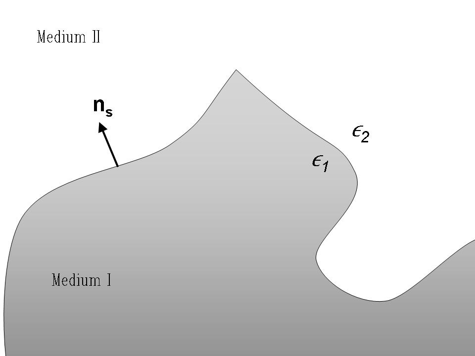
Figure 1: Interface between two regions with different dielectric constants $\epsilon_{1}$ and $\epsilon_{2}$ bounded by a surface S.

II Extended Theory

Here we investigate the electromagnetic modes localized at the surface $S$ separating two different media I-II, characterized by two dielectric constants $\epsilon_{1}$ and $\epsilon_{2}$ respectively. The normal vector ${\bf n_{s}}$ at the interface position ${\bf s}$ has been chosen arbitrarily to point towards medium II, see FIG. 1. In this way, we shall call ”internal” the variable defined in the part of space corresponding to medium I, and ”external” the variable defined in the part of space corresponding to medium II. For instance, $\epsilon_{1}$ will be denoted in the following by $\epsilon_{int}$ and $\epsilon_{2}$ by $\epsilon_{ext}$.

We want to obtain the surface plasmon modes of this system. These modes can be described by the Laplace equation for the quasi-static potential $u({\bf r})$ of the self field, everywhere except at the surface $S$ where we have the following equation

$$\nabla^{2}u({\bf r})=-\sigma({\bf r}),$$ (1)

with $\sigma({\bf r})$ the surface charge density, i.e. different from zero on the contour surface $S$. Let us note by ${\bf x}$ the position vectors located on the surface, therefore $\sigma({\bf x})$ is related to the normal derivatives of the potentials internal $u_{int}$ and external $u_{ext}$ to the surface $S$ by the following relation Abajo02

$$\sigma({\bf x})=\frac{\partial u_{int}}{\partial n_{x}}-\frac{\partial u_{ext}}{\partial n_{x}}.$$ (2)

The continuity equation for the self-fields at the boundary gives the following condition between the normal derivatives of the potential at any point of the surface $S$

$$\epsilon_{int}\frac{\partial u_{int}}{\partial n_{x}}=\epsilon_{ext}\frac{\partial u_{ext}}{\partial n_{x}}.$$ (3)

From the previous equations, we can recast Eq. (1) as follows

$$u({\bf x})=\int_{S}G({\bf x},{\bf x^{\prime}})\sigma({\bf x}^{\prime})dS({\bf x}^{\prime})$$

$$=\int_{S}G\left(\frac{\partial u_{int}}{\partial n}-\frac{\partial u_{ext}}{\partial n}\right)dS({\bf x}^{\prime})$$

$$=(1-\epsilon_{int}/\epsilon_{ext})\int_{S}G\frac{\partial u_{int}}{\partial n}dS({\bf x}^{\prime})$$ (4)

where $G({\bf x},{\bf x^{\prime}})=1/4\pi|{\bf x}-{\bf x^{\prime}}|$ is the Green function solution of the homogenous Laplace equation

$$\nabla^{2}G({\bf x},{\bf x^{\prime}})=-\delta({\bf x}-{\bf x^{\prime}})$$ (5)

where $\delta$ is the Dirac delta function.

Now considering a point ${\bf x}={\bf x}_{o}$ on the boundary S with possible singularities, and applying eqs. (A5) and (A6) of the appendix, i.e. evaluating the integral in Eq. (4) in Cauchy Principal Value sense, we obtain the following integral equationvincent09

$$u({\bf x}_{0})\left[\frac{\Omega({\bf x}_{0})}{4\pi}-\frac{\epsilon_{ext}}{\epsilon_{ext}-\epsilon_{int}}\right]$$

$$=\int_{S}u({\bf x}^{\prime})\left(-\frac{\partial G}{\partial n}({\bf x}_{0},{\bf x^{\prime}})\right)dS({\bf x}^{\prime})$$ (6)

where $\Omega({\bf x}_{0})$ is the solid angle sustained by the surface at the point ${\bf x}_{0}$.

Let us measure solid angles in units of $4\pi$($\hat{\Omega}\equiv\frac{\Omega}{4\pi}$) and define $\delta\hat{\Omega}=\hat{\Omega}-1/2$ as the deviation from a smooth surface. Notice that $\delta\hat{\Omega}<0$ for a surface with a protrusion (convex) and $\delta\hat{\Omega}>0$ for a concave surface. We can now write

$$\int_{S}d\hat{\Omega}({\bf x}_{0},{\bf x^{\prime}})u({\bf x^{\prime}})=\lambda u({\bf x}_{0})$$ (7)

where we have used the fact that $\int_{S}\left(-\frac{\partial G}{\partial n}\right)dS({\bf x}^{\prime})=\frac{\Omega({\bf x}_{0})}{4\pi}$, and consequently $d\hat{\Omega}({\bf x}_{0},{\bf x}^{\prime})$ is the normalized elementary solid angle sustained by $dS({\bf x}^{\prime})$ viewed from ${\bf x}_{0}$. To the best of our knowledge, the surface integral equation allowing to obtain the surface modes of the corresponding system was never written as a solid angle integral equation Eq.(7). This equation is pointing out the purely geometrical nature of these modes. We note that equation (7) is an exact expression, that complements recent numerical approximations Mayergoyz05 for smooth surfaces, and puts them into a more general context that includes surfaces with singularities.

Finally we interpret equation (7) as an eigenvalue equation where

$$\lambda\equiv[\lambda_{0}(\omega)+\delta\hat{\Omega}]$$ (8)

and we have defined the frequency factor

$$\lambda_{0}(\omega)=\frac{\epsilon_{ext}+\epsilon_{int}}{2(\epsilon_{int}-\epsilon_{ext})}=1/2-(\omega/\omega_{b})^{2}.$$ (9)

In the last line we have introduced the generic case of a Drude metal for $\epsilon_{int}$ with bulk plasma frequency $\omega_{b}$ and vacuum value for $\epsilon_{ext}$. Notice again that the right hand side of Equation (6) is entirely a geometric object. Furthermore, since the integral is evaluated in the Cauchy Principal Value sense its main singularity is already present in the factor $\delta\hat{\Omega}=\hat{\Omega}-1/2$.

Now let us consider the $\lambda=0$ eigenvalue

$$\epsilon_{ext}(1-\hat{\Omega})+\epsilon_{int}\hat{\Omega}=0$$ (10)

In the Drude limit of Eq.(9), we obtain the following for the plasmon energy $\omega$

$$(\omega/\omega_{b})^{2}=\hat{\Omega}.$$ (11)

III Results and discussion

The derivation of the previous section has shown the crucial connection between the shape and the spectral properties of the surface plasmon modes. In this section, for some selected geometries, we demonstrate the existence of the $\lambda=0$ eigenmode. Afterward, we apply Eq. (10) corresponding to the $\lambda=0$ case for metallic-vacuum interface, using a Drude dielectric response for the metal, and obtain the energies of these modes.

III.1 $\lambda=0$ mode for a semi-infinite metal

The planar interface is a well known geometry for its analytical solutions of the Laplace equation. For a semi-infinite metal, with ${\bf x}_{0}$ on the planar surface, any elementary solid angle of the surface, view from ${\bf x}_{0}$ vanishes ($d\hat{\Omega}({\bf x}_{0},{\bf x}^{\prime})=0$). Consequently any function defined only in the interface, will be solution of the integral equation (7), with eigenvalue $\lambda=0$. For a planar surface, as we are dealing with a smooth surface, we have $\hat{\Omega}=1/2$. Therefore applying Eq. (11), we obtain the well known infinitely degenerated surface plasmon mode of frequency $\omega_{s}=\omega_{b}/\sqrt{2}$.

III.2 Modes localized in one dimensional surface singularities

Now let us imagine a transformation, which generates from a smooth interface an interface with singularities, e.g., folding the previous planar interface along a straight line. In this way, we create a one dimensional straight singularity. Along the singularity, we can define a geometric solid angle. For example, let us consider a wedge of 90 degrees. In this case, the solid angle sustained by the surface at the singularity is $\pi$ ($\hat{\Omega}=1/4$), for the modes localized along the singularity, i.e. defined on the singularity only, the surface integral in Eq. (7) reduces to a line integral over the singularity. Any function defined along this straight singularity, only and anywhere else, will be solution of the line integral equation with the eigenvalue $\lambda=0$. Therefore using a Drude approximation of the dielectric constant of the metal and using Eq. (11), we obtain a plasmon wedge frequency $\omega_{s}=\omega_{b}/2$.

This derivation can be extended to a general wedge solid angle. Let it be $\alpha$ the interior angle defined by the intersection of two semi-infinite planes (see Fig. 2). In this case the solid angle sustained by the surface at the singularity is $2\alpha$ ($\hat{\Omega}=\alpha/2\pi$). Using Eq. (11), we obtain the plasmon wedge frequency $\omega_{s}=\omega_{b}\sqrt{\alpha/2\pi}$.

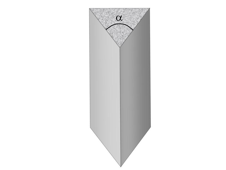
Figure 2: Wedge geometry with an interior angle $\alpha$.

III.3 Modes localized at a sharp point

Let us consider a point surface singularity, i.e., a metal vacuum interface with a sharp point. In this case, in Eq. (7), the integral over the singularity vanishes, giving also for the mode localized at the singularity, a $\lambda=0$ mode as the only possible solution.

For the conical geometry, where the full metallic cone is defined by the apex angle $2\alpha$, illustrated in figure Fig. (3), we calculate using Eq. (11), the frequency of the mode localized at the apex. The geometric solid angle is given by $\Omega_{s}=2\pi(1-\cos(\alpha))$, giving for the frequency of the mode, called here a dot plasmon $\omega_{b}$ mode:

$$\omega_{d}^{2}=\frac{1-\cos\alpha}{2}\omega_{b}^{2}$$ (12)

It is interesting to notice that for small angle, this mode becomes linearly angle dependent, $\omega_{d}\sim\omega_{b}\alpha/2$. These results are relevant due to the important role of the tip geometry, for the tip-enhanced spectroscopies, when the tip can can be modelized by a metallic cone.

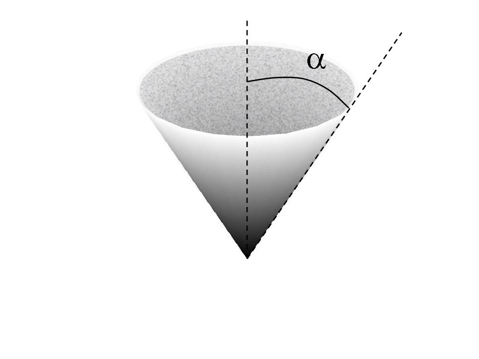
Figure 3: Conical geometry with an apex angle $2\alpha$.

These results are generalizable to modes localized at corners. Let us consider the corner at the intersection of three semi-infinite planes normal to each other, where the metallic part is filling $1/8$ of the space. We have at the intersection of the planes the solid angle of $\Omega_{s}=\pi/2$. Using equation (11), we obtain the frequency of the mode localized at the corner,

$$\omega_{d}=\frac{1}{2\sqrt{2}}\omega_{b}.$$ (13)

III.4 Complementarity rule

One of the important properties of the plasmon modes demonstrated in smooth surfaces is the complementarity rule that relates the plasmon energies of a system and those of its complementary Apell96 . Here, we are going to demonstrate that it can be generalized to surfaces with singularities. The important point, as it is obvious from Eq. (7), is that the eigenvalues of a system $\lambda(S)$ and the ones of its complementary $\lambda(\overline{S})$ are the same: vincent09

$$\lambda(\overline{S})=\lambda(S).$$ (14)

The reason is that the two systems show the same surface, the only difference is that the values of the dielectric constant at both sides of the surface are interchanged. In other words, to treat the complementary system, we just need to interchange the values of $\epsilon_{int}$ and $\epsilon_{ext}$ in Eq. (10). For a Drude metal, one finally obtains

$$\omega_{i}^{2}(S)+\omega_{i}^{2}(\overline{S})=\omega_{b}^{2}.$$ (15)

This rule is obviously applicable to any surface geometry, i.e., no matter it is a smooth surface or with a sharp singularity where a solid angle can be defined.

III.5 Extension to general dielectric materials

If the metal is not a Drude metal and/or the second medium is not vacuum, one can still get the plasmon frequencies using the more general equation(10). In this case, one can get the plasmon frequencies using experimental data for the dielectric function of both systemsPalik85 .

In table I, we summarize for the different cases explained above, the results for the plasmon frequencies obtained for Drude metals, and the conditions to be fulfilled by the ratio of the dielectric function at the plasmon frequencies when the more general (10) has to be used.

		Semi-infinite	Wedge($90^{\circ}$)	Wedge($\alpha$)	Corner($90^{\circ}$)	Dot plasmon($\alpha$)
		medium				conical
$(\omega/\omega_{b})^{2}$		1/2	1/4	$\alpha/2\pi$	1/8	$(1-\cos\alpha)/2$
$\epsilon_{int}/\epsilon_{ext}$		-1	-3	$1-2\pi/\alpha$	-7	$(\cos\alpha+1)/(\cos\alpha-1)$

Table 1: Comparison for different geometries of surface singularities squared of the plasmon energy divided by the bulk plasmon energy within the Drude model (see Eq. 11). Values of the ratio $\epsilon_{int}/\epsilon_{ext}$, between the interior and the exterior dielectric functions at the frequency of the surface plasmon for different geometries of surface singularities (see Eq. (10)).

IV Summary

Herein, we have derived a general framework (7-9) and simple geometrical rules Eq. (10-11) which determines surface plasmon energies and plasmon modes, based on the shape of the metal. The results presented here provide simple and straightforward rules to design the energy of surface plasmons in several situations of experimental interest such as in plasmon wave guiding and in tip-enhanced spectroscopies. We have shown applications of the rule to obtain the surface plasmon energies in wedges, corners and conical tips.

If the dispersion were included, one would be able to give valuable information for the plasmon wave guiding. Knowing that the framework of this theory allows to include it Mayergoyz05 , it will be a further point of interest in the future.

Appendix A General derivation of a gradient formulation of the laplace integral equation

Let us consider the partial differential equation

$$L(w)=0~{}in~{}B,$$ (16)

where B is a region in 3D-space with surface S, and L is a linear elliptic differential operator operating on a sufficiently smooth function w of 3D-variables ${\bf x}$. The Green’s reciprocal identity for the operator L can be written:

$$\int_{B}[uL(v)-v\bar{L}(u)]dB=\int_{S}\left(u\frac{\partial v}{\partial n}-v\frac{\partial u}{\partial n}\right)dS,$$ (17)

in which u and v are arbitrary functions, $\bar{L}$ is the operator adjoint to $L$ and $n$ is the outward normal to S. Let us choose v as the fundamental solution $G({\bf x},{\bf x^{\prime}})=1/4\pi|{\bf x}-{\bf x^{\prime}}|$ (in this case $L=\nabla^{2}$) such that:

$$L(G)=-\delta({\bf x}-{\bf x^{\prime}})$$ (18)

where $\delta$ is the Dirac delta function. The integrands in Eq.(A2) can be expanded as an appropriate limit process Muskhelishvili53 . We therefore consider a point ${\bf x}={\bf x}_{o}$ on the boundary S and let there be a sphere around this point separating a volume $B_{\rho}$ and surface $S_{\rho}$ from the rest of B. Let $B_{0}$ denote what is left of region B with surface $S_{0}$ comprised of $S_{1}$ and $S_{\rho}$ according to the Fig. 4

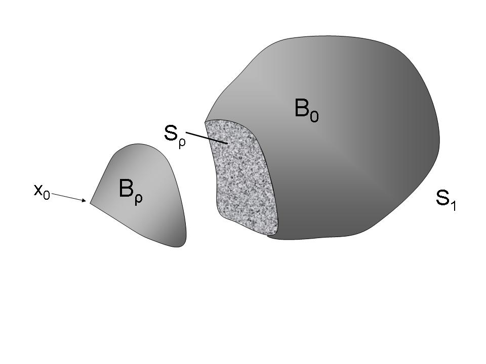
Figure 4: Segment $B_{\rho}$ and the remainder $B_{0}$ of the region $B$.

Evaluating Eq.(A3) for $B_{0}$ and $S_{0}$ , which does not contain the point ${\bf x}_{0}$, only the surface integral is left:

$$0=\int_{S_{0}}\left(G\frac{\partial u}{\partial n}-u\frac{\partial G}{\partial n}\right)dS(x^{\prime})$$ (19)

The first term of Eq. (A4) has a singularity which is integrable, while the second term has to be treated with more care. Splitting the integral over $S_{0}$ as $S_{1}$ and $S_{\rho}$ and adding/subtracting $u({\bf x}_{0})$, and in the limit $\rho\rightarrow 0$, we get the main result in HARTMANN81 (for ${\bf x}_{0}$ on the boundary):

$$c({\bf x}_{0})u({\bf x}_{0})=\int_{S}\left(G\frac{\partial u}{\partial n}-u\frac{\partial G}{\partial n}\right)dS(x^{\prime})$$ (20)

where the second integral is to be interpreted in Cauchy Principal Value sense. Obviously by setting $u=1$ we have:

$$c({\bf x}_{0})=\int_{S}\left(-\frac{\partial G}{\partial n}\right)dS(x^{\prime})=\frac{\Omega({\bf x}_{0})}{4\pi}$$ (21)

where we have used that $\Omega({\bf x}_{0})$ is the solid angle pertaining to the point ${\bf x}_{0}$.

- (1) E. Devaux J.-Y. Laluet S. I. Bozhevolnyi, V. S. Volkov and T. W. Ebbesen. Nature, 440: 508-511, (2006).
- (2) F. B. Segerink T. H. Taminiau, F. D. Stefani and N. F. van Hulst. Nature Photonics, 2: 234-237, (2008).
- (3) E. Prodan and P. Nordlander. Nano Letters, 3(4): 543-547, (2003).
- (4) D. R. Ward, N. K. Grady, C. S. Levin, N. J. Halas, Y. Wu, P. Nordlander, and D. Natelson. Nano Letters, 7(5): 1396-1400, (2007).
- (5) H. Szmacinski and J. R. Lakowicz. Sensors and Actuators B: Chemical, 29(1-3): 16 - 24, (1995).
- (6) K. Aslan, J. R Lakowicz, and C. D. Geddes. Current Opinion in Chemical Biology, 9(5): 538 -544, (2005).
- (7) S. Lal, S. E. Clare, and N. J. Halas. Accounts of Chemical Research, 41(12): 1842-1851, (2008).
- (8) G. Mie. Ann. Phys. (Leipzig), 25: 377, (1908).
- (9) F. J. Garcia de Abajo and J. Aizpurua, Phys. Rev. B, 56(24): 15873-15884, (1997).
- (10) A. Farjadpour, D. Roundy, A. Rodriguez, M. Ibanescu, P. Bermel, J. D. Joannopoulos, S. G. Johnson, and G. Burr. Optics Letters, 31: 2972-2974, (2006).
- (11) M.A. Yurkin and A.G. Hoekstra , 106(1-3): 558 - 589, (2007). IX Conference on Electromagnetic and Light Scattering by Non-Spherical Particles.
- (12) F.J. Garcia de Abajo, and A. Howie, Phys. Rev. B 65, 115418 (2002).
- (13) R.P. Vincent, PhD Thesis, University of the Basque Country (2009).
- (14) I.D. Mayergoyz, D. R. Fredkin, Z. Zhang, Phys. Rev. B 72, 155412 (2005).
- (15) S.P. Apell, P.M. Echenique, R.H. Ritchie, Ultramicroscopy 65, 53-60 (1996).
- (16) E. D. Palik, Handbook of Optical Constants of Solids (Academic, New York, 1985).
- (17) E.J. Scott, N. I. Muskhelishvili, Singular integral equations. 2nd ed. Groningen, P. Noordhoff, Ltd., (1953).
- (18) F. Hartmann, Journal of Elasticity, 11, No. 4 (1981)