Chiral properties of strong interactions in a magnetic background

Abstract

We investigate the chiral properties of QCD in presence of a magnetic background field and in the low temperature regime, by lattice numerical simulations of $N_{f}=2$ QCD. We adopt a standard staggered discretization, with a pion mass around 200 MeV, and explore a range of magnetic fields $(180\ {\rm MeV})^{2}\leq|e|B\leq(700\ {\rm MeV})^{2}$, in which we study magnetic catalysis, i.e. the increase of chiral symmetry breaking induced by the background field. We determine the dependence of the chiral condensate on the external field, compare our results with existing model predictions and show that a substantial contribution to magnetic catalysis comes from the modified distribution of non-Abelian gauge fields, induced by the magnetic field via dynamical quark loop effects.

I Introduction

The study of strong interactions in presence of a strong background magnetic field has attracted increasing attention in the recent past. On one side the issue is of great phenomenological relevance: magnetic fields of the order of $10^{16}$ Tesla, i.e. $\sqrt{|e|B}\sim 1.5$ GeV) may have been produced at the cosmological electroweak phase transition Vachaspati:1991nm and they may have influenced subsequent strong interaction dynamics, including the confinement/deconfinement transition. Slightly lower fields are expected to be produced in non-central heavy ion collisions (up to $10^{14}$ Tesla at RHIC and up to $\sim 10^{15}$ Tesla at LHC heavyionfield1 ; heavyionfield2 ), where they may give rise to new phenomenology, the so-called ”chiral magnetic effect”, capable of revealing the presence of deconfined matter and of non-trivial topological vacuum fluctuations cme0 ; cme1 ; star . Finally, magnetic fields of the order of $10^{10}$ Tesla are expected to be present in a class of neutron stars known as magnetars magnetars (for a recent review see Ref. mereghetti ).

On the other side, a background magnetic field (electro-magnetic or chromo-magnetic) may serve as yet another parameter to probe the structure of the QCD vacuum and of the QCD phase diagram, on the same footing with other interesting external conditions such as a baryon chemical potential. Many studies salam ; linde ; Kawati:1983aq ; Klevansky:1989vi ; Suganuma ; Klimenko ; Schramm ; Klimenko:1993ec ; Gusynin:1994re ; Gusynin:1994xp ; Shushpanov:1997sf ; Babansky:1997zh ; Ebert ; Goyal:1999ye ; Agasian:1999sx ; Ebert:2001ba ; Kabat:2002er ; Miransky:2002rp ; Cohen:2007bt ; Johnson:2008vna ; Rojas ; Bergman:2008qv ; Zayakin:2008cy ; Evans:2010xs ; mizher ; Nam have investigated the chiral properties of the theory and what is generally known as magnetic catalysis, consisting in an enhancement of chiral symmetry breaking and in spontaneous mass generation induced by the magnetic field, a phenomenon predicted from different low energy models and approximations of QCD and related to the dimensional reduction taking place in the dynamics of particles moving in a strong external magnetic field Gusynin:1994re ; Gusynin:1994xp ; Miransky:2002rp . More recently, the issue of the influence of a magnetic field on the deconfinement transition has been investigated by means of both lattice QCD simulations and low energy models of strong interactions Klimenko ; Nam ; agasian ; fraga1 ; Avancini ; Ayala ; NJL ; fukushima ; fraga2 ; demusa ; gatto1 ; frolov ; sadooghi ; gatto2 ; Preis:2010cq : there is converging evidence that a magnetic field leads to an increase of both the strength and the temperature of the transition; in the case of a chromo-magnetic field, instead, numerical simulations show a decrease of the transition temperature bari1 ; bari2 . Finally, conjectures have been proposed according to which a strong enough magnetic field may induce the appearance of new superconductive phases supercond1 ; supercond2 ; supercond3 .

In the present study we address the issue of magnetic catalysis, presenting the first study of such phenomenon by lattice QCD simulations which include the contribution of dynamical quarks; previous numerical studies indeed have only considered the effect of the magnetic field on quenched configurations itep1 ; itep2 . In particular, we have considered QCD at zero or low temperature, with two dynamical flavors carrying different electric charges, corresponding respectively to the $u$ and $d$ quark charges, and coupled to a background constant and uniform magnetic field. We have adopted a standard rooted staggered fermion discretization,with a (Goldstone) pion mass of about 200 MeV.

One of the purposes of our investigation is to obtain information about the dependence of the chiral condensate on the magnetic field, and compare it with various existing model and low energy predictions. A second purpose that we have is to understand which part of magnetic catalysis is a purely tree level effect, due to the fact that quarks propagate in a modified background obtained by adding the U(1) field to the non-Abelian gauge configurations, and which part is due to a modification of the non-Abelian fields themselves, induced by the loop effects of dynamical quarks coupled to the magnetic background. Both effects can in principle modify the spectrum of the Dirac operator, leading to a larger density of eigenvalues around zero, hence to an increase of the chiral condensate via the Banks – Casher relation banks .

To that aim, one could compare with existing investigations of magnetic catalysis, based on SU(2) and SU(3) gauge configurations sampled by pure gauge simulations itep1 ; itep2 : however that would not be completely satisfactory and would also be difficult because of different scale settings and renormalization effects. What we will do instead is to try separating the two different effects, by inserting alternatively the magnetic field only in the computation of the quark propagator (sampling in this case configurations without the presence of the magnetic field), or only in the sampling measure, i.e. in the fermion determinant, without affecting the quark propagator computation. We will call ”valence” catalysis the first contribution and ”dynamical” catalysis the second: both of them will be compared with the full increase of the chiral condensate, obtained when the magnetic field is inserted directly both in the fermion determinant and in the computation of the quark propagator. As we will show, the purely dynamical contribution corresponds to a considerable part of the total increase in the quark condensate.

The paper is organized as follows. In Sec. II we give some details about our lattice discretization of QCD in presence of a magnetic field and about our numerical setup. In Section III we present our numerical results and finally, in Section IV, we give our conclusions.

II Numerical Setup

The discretization of $N_{f}=2$ QCD in presence of a magnetic background field adopted in the present work is similar to that reported in Ref. demusa . In particular, partition function of the (rooted) staggered fermion discretized version of the theory in presence of a non-trivial electro-magnetic (e.m.) background field and with different electric charges for the two flavors, $q_{u}=2|e|/3$ and $q_{d}=-|e|/3$ ($|e|$ being the elementary charge), is written as:

$$Z(T,B)\equiv\int\mathcal{D}Ue^{-S_{G}}\det M^{1\over 4}[B,q_{u}]\det M^{1\over 4}[B,q_{d}]\>$$ (1)

$$M_{i,j}[B,q] = am\delta_{i,j}+{1\over 2}\sum_{\nu=1}^{4}\eta_{i,\nu}\left(\vphantom{U^{{\dagger}}_{i-\hat{\nu},\nu}}u(B,q)_{i,\nu}U_{i,\nu}\delta_{i,j-\hat{\nu}}\right.$$ (2)

$$-\left.u^{*}(B,q)_{i-\hat{\nu},\nu}U^{{\dagger}}_{i-\hat{\nu},\nu}\delta_{i,j+\hat{\nu}}\right)\>.$$

$\mathcal{D}U$ is the functional integration over the non-Abelian gauge link variables $U_{n,\mu}$, $S_{G}$ is the discretized pure gauge action (we consider a standard Wilson action); $u(B,q)_{i,\nu}$ are instead the Abelian gauge links corresponding to the background e.m. field. The subscripts $i$ and $j$ refer to lattice sites, $\hat{\nu}$ is a unit vector on the lattice and $\eta_{i,\nu}$ are the staggered phases. Periodic (antiperiodic) boundary conditions (b.c.) must be taken, in the finite temperature theory, for gauge (fermion) fields along the Euclidean time direction, while spatial periodic b.c. are chosen for all fields.

We shall consider a constant and uniform magnetic field $\vec{B}=B\hat{z}$. The presence of periodic b.c. in the $x$ and $y$ directions imposes a constraint on the admissible values of $B$, which get quantized, as illustrated in the following subsection. Symmetry under charge conjugation imposes that $Z(T,B)$ as well as other charge even observables, including the chiral condensate, be even functions of $B$.

II.1 Magnetic Field on a Torus

In presence of periodic b.c., the magnetic field in the $z$ direction goes through the surface of a torus in the $x-y$ directions, whose total extent is $l_{x}l_{y}$. The circulation of $A_{\mu}$ along any closed path, lying in the $x-y$ plane and enclosing an arbitrary region of area $A$ (see e.g. Fig. 1), is proportional, by Stokes’ theorem, to the flux of $B$ through the enclosed surface

$$\oint A_{\mu}dx_{\mu}=AB$$ (3)

On the other hand, since we are on a torus, it is ambiguous to state which is the enclosed surface: the complementary region of area $l_{x}l_{y}-A$ can be chosen as well, therefore one can equally state

$$\oint A_{\mu}dx_{\mu}=(A-l_{x}l_{y})B\,.$$ (4)

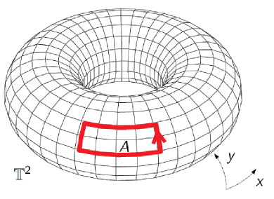
Figure 1: Surface with periodic b.c. orthogonal to the direction of the magnetic field. The phase factor taken by a particle moving around the plotted countour must be defined unambiguously and this leads to magnetic flux quantization.

At the level of the gauge field the ambiguity is resolved by admitting discontinuities in $A_{\mu}$ somewhere on the torus, or alternatively by covering the torus with various patches where different gauge choices are taken. In any case, one has to guarantee that the ambiguity is not visible by charged particles moving on the torus, and this is true only if the phase factor taken by the charged particle moving along the closed path is defined unambiguously

$$\exp\left(iqBA\right)=\exp\left(iqB(A-l_{x}l_{y})\right)$$ (5)

i.e. if

$$qB=2\pi b/l_{x}l_{y}$$ (6)

where $b$ is an integer. Notice that this line of argument is exactly the same that applies on a sphere and that leads to Dirac quantization of the magnetic monopole charge. The quantization rule depends on the electric charge of the particles feeling the presence of the magnetic field, in particular it is set by the smallest charge unit, which in our case is brought by the $d$ quark, $q_{d}=-|e|/3$, hence

$$|e|B=6\pi b/l_{x}l_{y}=6\pi ba^{-2}/L_{x}L_{y}$$ (7)

where $L_{x}$ and $L_{y}$ are the system sizes in lattice units and $a$ is the lattice spacing.

Further details about the definition of a magnetic field on a torus can be found in Ref. wiese , where it is shown that translational invariance on the torus is explicitly broken by the presence of the magnetic field, due to the non-trivial phases taken by particles winding around one of the directions of the torus (Wilson lines): only a discrete invariance is left, by shifts which are integer multiples of

$$a_{x}=l_{x}/b\,\,\,;\,\,\,\,\,\,\,\,a_{y}=l_{y}/b$$ (8)

respectively in the $x$ and $y$ directions. Such invariance is reduced further on a lattice, since only shifts, if any, which are multiples of both $a_{x}$ ($a_{y}$) and the lattice spacing $a$ leave the system invariant: that may lead to additional discretization effects.

II.2 Discretization details

We have taken the following choice for the continuum e.m. gauge field:

$$A_{y}=Bx\>;\qquad\qquad A_{\mu}=0\quad\mathrm{for}\quad\mu=x,z,t\>.$$ (9)

The corresponding $U(1)$ links on the lattice are:

$$u(B,q)_{n,y}=e^{ia^{2}qBn_{x}}\,;\,\,\,u(B,q)_{n,\mu}=1\>\mathrm{for}\>\mu=x,z,t\$$ (10)

In order to guarantee the smoothness of the background field across the boundary and the gauge invariance of the fermion action, the $U(1)$ gauge fields must be modified at the boundary of the $x$ direction:

$$u(B,q)_{n,x}|_{n_{x}=L_{x}}=e^{-ia^{2}qL_{x}Bn_{y}}\>$$ (11)

and the magnetic field must be quantized as specified in Eq. (7). That corresponds to taking the appropriate gauge invariant b.c. for fermion fields on the torus wiese (with the possible additional free phases $\theta_{x}$ and $\theta_{y}$ wiese set to zero).

We have considered a symmetric lattice, $L_{x}=L_{y}=L_{z}=N_{t}=16$, a bare quark mass $am=0.01335$ and an inverse gauge coupling $\beta=5.30$. According to scale estimates reported in Ref. demusa , that corresponds to a lattice spacing $a\simeq 0.3$ fm, a (Goldstone) pion mass $m_{\pi}\simeq 200$ MeV and a temperature $T=(N_{t}a)^{-1}\simeq 40$ MeV, hence low enough that the system can be considered to be effectively at zero temperature.

We have explored different values of $|e|B$ which, according to Eq. (7), can be changed only in units of $6\pi a^{-2}/L_{x}L_{y}\simeq(180$ MeV)². Notice however that the presence of an ultra-violet (UV) cutoff imposes also an upper limit on the possible values of $B$ that can be explored on the lattice. To appreciate that, let us consider again the phase factor picked up by a particle moving around a closed path in the $x-y$ plane, and which contains all the relevant information about the effect of the magnetic field on particle dynamics: there is a minimal such path on the lattice, corresponding to a plaquette, around which the particle takes the phase factor

$$\exp(iqa^{2}B)=\exp\left(\frac{i2\pi b}{L_{x}L_{y}}\right)\,.$$ (12)

The phase factor above, and therefore all other phase factors associated to any closed lattice path, cannot distinguish magnetic fields such that $qa^{2}B$ differs by multiples of $2\pi$. One can therefore define a sort of ”first Brillouin zone” for the magnetic field,

$$-\frac{\pi}{a^{2}}<qB<\frac{\pi}{a^{2}}$$ (13)

i.e.

$$-\frac{L_{x}L_{y}}{2}<b<\frac{L_{x}L_{y}}{2}\,,$$ (14)

with all physical quantities being periodic in $qB$ $(b)$ with a period $2\pi/a^{2}$ ($L_{x}L_{y}$); symmetry under $b\to-b$ further reduces the range of interesting values of $b$. Even before reaching the limits reported in Eq. (13), one expects the periodicity to induce saturation effects, which may distort the true physical dependence of observables, like the chiral condensate, on $B$. One should always worry about the possible presence of such saturation effects, when trying to extract information relevant to continuum physics.

II.3 Observables and simulation details

The quantity which is the subject of our investigation is the chiral condensate. In presence of a non-zero $B$ we can define two different condensates

$$\Sigma_{u/d}(B) \equiv \frac{\partial\log Z}{\partial m_{u/d}}|_{m_{u/d}=m}$$

$$= \int\mathcal{D}U{\cal P}[m,U,B]{\rm Tr}\left(M^{-1}[m,B,q_{u/d}]\right)$$

where the functional integral measure is (see Eq. (1)):

$${\cal P}[m,U,B]\propto\det M^{1\over 4}[m,B,q_{u}]\det M^{1\over 4}[m,B,q_{d}]e^{-S_{G}}$$ (16)

A quantity which is useful to discuss magnetic catalysis is the relative increment of the quark condensate, which we define as:

$$r_{u/d}(B)\equiv\frac{\Sigma_{u/d}(B)}{\Sigma(0)}-1=\frac{\Sigma_{u/d}(B)-\Sigma(0)}{\Sigma(0)}\,.$$ (17)

The advantage of $r(B)$ is that it is a dimensionless quantity and that most renormalizations appearing in the definition of $\Sigma$ cancels out in Eq. (17). Indeed, assuming that renormalizations have a negligible dependence on $B$, as should be the case as long as $B$ stays away from the scale of the UV cutoff, the mass dependent additive renormalization of $\Sigma$ will cancel out in the numerator of Eq. (17). A residual additive renormalization remains in the denominator, leading to an incorrect overall normalization of $r(B)$: in the following we shall try to estimate the magnitude of such systematic error.

We shall define flavor averaged quantities as well:

$$\Sigma(B)=\frac{\Sigma_{u}(B)+\Sigma_{d}(B)}{2}$$ (18)

and

$$r(B)=\frac{\Sigma(B)}{\Sigma(0)}-1=\frac{r_{u}(B)+r_{d}(B)}{2}$$ (19)

Both $\Sigma_{u}(B)$ and $\Sigma_{d}(B)$ are, by charge conjugation symmetry, even functions of $B$. Moreover, according to what discussed in Sec. II.2, they are expected to be periodic in $B$, with a period $2\pi a^{-2}/q_{d}$ (or alternatively with a period $L_{x}L_{y}$ in terms of the quantum number $b$ defined in Eq. (6)). One could expect the $u$ quark condensate to have a periodicity shorter by a factor 2, since $|q_{u}|=2|q_{d}|$, however this is not exactly true because of the measure ${\cal P}[m,U,B]$ appearing in Eq. (II.3), whose periodicity is set by the quark with the lower charge.

In the limit $m\to 0$ the chiral condensate is an order parameter for chiral symmetry breaking and is related by the Banks - Casher relation banks to the density $\rho(\lambda)$ of eigenvalues of the Dirac operator, $D=M-m\ {\rm Id}$, around $\lambda=0$: $\Sigma=\pi\rho(0)$. On the contrary, for $m\neq 0$, the chiral condensates defined in Eq. (II.3) are not related to the densities of zero eigenvalues of the respective Dirac operators, $\rho_{u/d}(0)$, which instead can be obtained by taking the limit $m\to 0$ only for the trace term appearing in Eq. (II.3), i.e.

$$\rho_{u/d}(0)=\frac{1}{\pi}\lim_{m^{\prime}\to 0}\int\mathcal{D}U{\cal P}[m,U]{\rm Tr}\left(M^{-1}[m^{\prime},q_{u/d}]\right)$$ (20)

where the dependence on $B$ has been left implicit. We shall consider also such quantities and the corresponding relative increments

$$\tilde{r}_{u/d}\equiv\rho_{u/d}(0,B)/\rho(0,B=0)-1\,.$$ (21)

As discussed in the introduction, we are also interested in studying contributions to magnetic catalysis coming separately either from the change in the observable ${\rm Tr}\left(M^{-1}[m,B,q_{u/d}]\right)$ (”valence” contribution), or from that in the measure ${\cal P}[m,U,B]$ (”dynamical” contribution). For that reason we define also:

$$\Sigma^{val}_{u/d}(B)\equiv\int\mathcal{D}U{\cal P}[m,U,0]{\rm Tr}\left(M^{-1}[m,B,q_{u/d}]\right)$$ (22)

and

$$\Sigma^{dyn}_{u/d}(B)\equiv\int\mathcal{D}U{\cal P}[m,U,B]{\rm Tr}\left(M^{-1}[m,0,q_{u/d}]\right)\,.$$ (23)

In the first case we look at the spectrum of the fermion matrix which includes the magnetic field explicitly, but is defined on non-Abelian configurations sampled at $B=0$. In the second case we look at the spectrum of the fermion matrix without an explicit magnetic field, but defined on gauge configurations sampled in presence of the magnetic field. From $\Sigma^{val}_{u/d}(B)$ and $\Sigma^{dyn}_{u/d}(B)$ we can define the corresponding quantities, $\Sigma^{val/dyn},r_{u/d}^{val/dyn},r^{val/dyn}$, analogously to what done in Eqs. (17), (18) and (19).

On general grounds we may expect that, in the limit of small fields, $B$ acts as a perturbation for both the measure term ${\cal P}[m,U,B]$ and the observable ${\rm Tr}\left(M^{-1}[m,B,q_{u/d}]\right)$ in Eq. (II.3). Given that both functions are even in $B$ and assuming they are also analytic (this may not be true in some limits, see discussion below), so that the first non-trivial term in $B$ is quadratic, one can write, configuration by configuration:

$${\cal P}[m,U,B]={\cal P}[m,U,0]+C\ B^{2}+O(B^{4})$$ (24)

and

$${\rm Tr}\left(M^{-1}[B]\right)={\rm Tr}\left(M^{-1}[0]\right)+C^{\prime}\ B^{2}+O(B^{4})\,$$ (25)

where it is assumed implicitly that the two constants $C$ and $C^{\prime}$ depend on the quark mass and on the chosen configuration. Putting together the two expansions one obtains

$$\frac{\Sigma_{u/d}(B)}{\Sigma(0)}-1=r^{val}_{u/d}(B)+r^{dyn}_{u/d}(B)+O(B^{4})\,.$$ (26)

Therefore, at least in the limit of small fields, the separation of magnetic catalysis in a valence part and in a dynamical part is a well defined concept. As we will show in the following, that continues to be true, within a good approximation, for a large range of fields explored in the present study. Notice that an approximate additivity of $r^{val}$ and $r^{dyn}$, like in Eq. (26), would be true also for different small field dependences, e.g. linear, in Eq. (24) and Eq. (25); hence the assumption above is stronger and also implies that magnetic catalysis should be a quadratic effect in $B$, at least for small fields and if the partition function is analytic in $B=0$.

We have made use of a Rational Hybrid Monte-Carlo algorithm to simulate rooted staggered fermions. Typical statistics are of the order of 3k thermalized molecular dynamics trajectories for each value of the magnetic field. The trace of the inverse of the fermion matrix, appearing in Eq. (II.3), has been computed, for each quark flavor, by means of a noisy estimator, extracting 10 random vectores for each configuration and for each value of the parameters. Numerical simulations have been performed on the apeNEXT facilities in Rome.

$b$	$r_{u}(b)$	$r_{d}(b)$	$r^{val}_{u}(b)$	$r^{val}_{d}(b)$	$r^{dyn}_{u/d}(b)$
1	0.0005(18)	-0.001(2)	0.0017(20)	0.0008(20)	-0.001(2)
2	0.0077(19)	0.0022(20)	0.0070(19)	0.0027(18)	0.0003(21)
3	0.0202(16)	0.0077(18)	0.0151(20)	0.0037(19)	0.0046(21)
4	0.0356(22)	0.0162(23)	0.0266(19)	0.0052(19)	0.0097(23)
5	0.0567(18)	0.0274(20)	0.0407(19)	0.0121(19)	0.0162(26)
6	0.0760(19)	0.0358(20)	0.0579(20)	0.0165(18)	0.0182(23)
7	0.0996(16)	0.0481(16)	0.0759(20)	0.0217(19)	0.0273(18)
8	0.1246(17)	0.0613(18)	0.0949(19)	0.0281(19)	0.0361(20)
9	0.1474(16)	0.0717(18)	0.1144(19)	0.0352(18)	0.0413(18)
10	0.1736(17)	0.0864(17)	0.1340(19)	0.0412(18)	0.0470(19)
11	0.2005(18)	0.1021(18)	0.1554(19)	0.0503(19)	0.0594(23)
12	0.2258(16)	0.1173(16)	0.1765(19)	0.0584(19)	0.0655(19)
13	0.2501(17)	0.1312(17)	0.1983(20)	0.0676(18)	0.0733(22)
14	0.2737(18)	0.1450(17)	0.2192(20)	0.0762(20)	0.0802(25)
16	0.3227(19)	0.1769(18)	0.2568(20)	0.0957(19)	0.0971(21)
24	0.4636(23)	0.2830(25)	0.3809(21)	0.1777(19)	0.1399(34)
32	0.5462(22)	0.3727(22)	0.4472(24)	0.2594(21)	0.1722(28)
48	0.6485(22)	0.5053(22)	0.5308(23)	0.3816(21)	0.2027(28)
64	0.6855(23)	0.5790(23)	0.5652(24)	0.4460(21)	0.2199(30)
80	0.6545(22)	0.6198(23)	0.5317(23)	0.4924(22)	0.2159(28)
96	0.5726(21)	0.6504(22)	0.4480(22)	0.5297(22)	0.2128(26)
112	0.3868(19)	0.6589(22)	0.2603(21)	0.5549(23)	0.1876(22)
128	0.1333(18)	0.6376(22)	0.0000(19)	0.5642(22)	0.1358(25)
144	0.3828(21)	0.6567(22)	0.2583(21)	0.5558(22)	0.1848(23)

Table 1: Relative increment of the $u$ and $d$ quark condensates for various magnetic field values. We report full data, as well as valence and dynamical contributions separately.

III Numerical Results

We report in Table 1 the relative increments of the $u$ and $d$ quark condensates respectively, including also measurements of the valence and of the dynamical contribution. Notice that $r^{dyn}(B)$ is exactly the same, by definition, for $u$ and $d$ quarks, since in this case the magnetic field affects only the fermion determinants. One can also explicitly verify from the table that $r^{val}_{u}(B/2)=r^{val}_{d}(B)$ within errors: this is expected since $|q_{u}|=2|q_{d}|$ and since in this case the sampling measure is independent of $B$.

As stressed in Section II.3, all definitions of $r$ are affected by a systematic overall normalization factor, due to an additive, mass dependent renormalization present in the condensate computed at zero magnetic field, $\Sigma(0)$ (see Eq. (17)). In order to estimate the magnitude of such systematic effect, we have performed simulations at $B=0$ and different values of the quark mass, keeping the lattice size unchanged, in order to determine the dependence of $\Sigma(B=0,m)$ on $m$; results are reported in Fig. 2. The expected leading order dependence on $m$ in the chirally broken phase is the following (see e.g. the discussion in Ref. ejiri ):

$$\Sigma(B=0,m)=\Sigma(0,0)+c_{1/2}\sqrt{m}+c_{1}m+O(m^{3})$$ (27)

where the non-analytic square root term is expected from the presence of Goldstone mode fluctuations gold1 ; gold2 ; gold3 , while the leading order, quadratically divergent contribution to the additive renormalization affects the linear term in $m$. A fit according to Eq. (27) gives $\Sigma(B=0,0)=0.565(6)$, $c_{1/2}=0.61(9)$ and $c_{1}=2.9(4)$, with $\chi^{2}/{\rm d.o.f.}=5.7/7$, from which we infer that the linear term in $m$ accounts for about 6% of the total signal measured at the quark mass explored in our investigation, i.e. $am=0.01335$.

We conclude that our determinations of $r$, $r^{val}$ and $r^{dyn}$ are distorted by a common and $B$ independent overall normalization factor, which leads to a systematic effect of the order of 10% and does not affect issues such as the separation of magnetic catalysis into a valence and dynamical contribution, as discussed later in this Section.

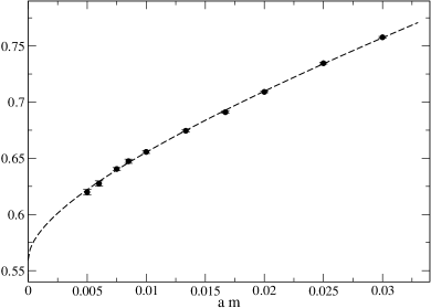
Figure 2: Dependence of the chiral condensate on the bare quark mass at $B=0$, together with a best fit curve according to Eq. (27).

III.1 Periodicity and saturation effects

In Fig. 3 we report results for the normalized condensates $\Sigma_{u/d}(B)/\Sigma(B)$ (i.e. $1+r_{u/d}(B)$) over the whole range of possible independent values of $B$, i.e. for $b/(L_{x}L_{y})$ ranging from 0 to 1 (see discussion at the end of Sec. II.2). Notice that data reported for $b/(L_{x}L_{y})\geq 0.625$ are not the result of direct simulations, but have been obtained by enforcing the expected invariances under $b\to b+L_{x}L_{y}$ (i.e. the above mentioned periodicity) and under $b\to-b$, which put together mean invariance under $b/(L_{x}L_{y})\to 1-b/(L_{x}L_{y})$. However, such invariance has been verified explicitly for a couple of points, $b/(L_{x}L_{y})=0.4375$ and $b/(L_{x}L_{y})=0.5625$, for which independent simulations have been performed.

Saturation effects, which are present for large values of $B$, are clearly visible from Fig. 3, where we have also reported for comparison the results of two fits to the small $B$ region. In particular, we infer from the figure that one should keep $b/(L_{x}L_{y})$ well below 0.1 in order that such effects stay negligible: that means $|e|B$ below $1/a^{2}\sim(700\ {\rm MeV})^{2}$ in our case. In the following only data obtained for $b\leq 16$ will be considered as reasonably free of saturation effects.

Notice that the $u$ quark condensate shows an approximate periodicity in $B$ which is halved with respect to the $d$ quark. That comes from the fact that $|q_{u}|=2|q_{d}|$ and is only approximate since instead the measure term has the usual periodicity. For instance $r_{u}(b)$ has a minimum but is not exactly zero at $b/(L_{x}L_{y})=1/2$, where the effective magnetic field felt by $u$ quarks is zero: there is a residual catalysis induced by dynamical $d$ quarks, which instead at $b/(L_{x}L_{y})=1/2$ feel the maximum possible magnetic field; for the same reason $r_{d}(b)$ does not reach its maximum at $b/(L_{x}L_{y})=1/2$. Such effects, which are absent for the purely valence contribution as can be checked from Table 1, are a first example of the dynamical contribution to magnetic catalysis, which we discuss in detail in the next subsection.

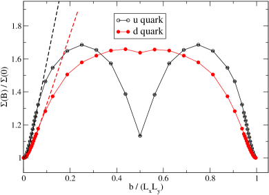
Figure 3: Normalized $u$ and $d$ quark condensates as a function of the magnetic field for the whole range of independent possible values of $B$. Data for $b/(L_{x}L_{y})>0.6$ have been obtained by enforcing the expected symmetry of the chiral condensate under $b/(L_{x}L_{y})\to 1-b/(L_{x}L_{y})$, while such symmetry has been verified for a couple of points, $b/(L_{x}L_{y})=0.4375$ and $b/(L_{x}L_{y})=0.5625$. We also report two curves corresponding to best fits in the small field region, to better show the presence of saturation effects.

III.2 Dynamical and Valence contributions to magnetic catalysis

In Fig. 4 we report the functions $r(B),r^{val}(B),r^{dyn}(B)$ (see Eqs. (22) and (23)) as well as the sum $r^{val}(B)+r^{dyn}(B)$, in order to appreciate the amount of magnetic catalysis caused by the modified distribution of the non-Abelian gauge fields, induced by the coupling of dynamical quarks to the magnetic field (dynamical contribution). We have limited our analysis to $b\leq 16$, for which saturation effects do not play a significant role.

The first thing that we notice is that the dynamical and valence contributions are roughly additive, in the sense that their sum gives back to full signal, in the range of fields shown in the figure. The additivity, which is expected in the limit of small fields (see discussion in Sec. II.3), is verified within errors for $b\leq 8$ ($|e|B\leq(500\ {\rm MeV})^{2}$), while small deviations appear beyond. Notice that this threshold coincides with that above which a purely quadratic fit for $r(B)$ does not work (see next subsection) and quartic terms in $B$ become important, in agreement with the argument given in Sec. II.3.

Once clarified that it is sensible, in the explored range of fields, to divide magnetic catalysis into a valence and a dynamical contribution, from Fig. 4 we learn that the dynamical one is roughly 40% of the total signal, at least for the discretization and quark mass spectrum adopted in our investigation. That means that numerical studies in which the magnetic field is not included in the sampling distribution (quenched or partially quenched) may miss a substantial part of magnetic catalysis, in a measure larger than other systematic effects due to quenching, which are typically of the order of 20%.

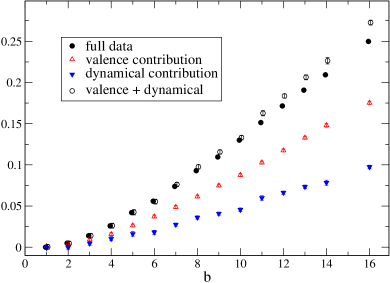
Figure 4: Relative increment of the average of the $u$ and $d$ quark condensates as a function of the magnetic field. We report separately $r(B),r^{val}(B),r^{dyn}(B)$ and $r^{val}(B)+r^{dyn}(B)$.

In Fig. 5 we have also plotted results for the difference between the $u$ and the $d$ condensates, which increases as a function of $B$, indicating an increasing breaking of flavor symmetry. The fact that the dynamical contribution is equal for the two quarks and the approximate additivity discussed above implies that such difference should be roughly unchanged if we consider just the valence contribution: that can be verified again from Fig. 5.

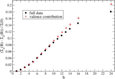
Figure 5: Difference of the $u$ and $d$ quark condensates, normalized by the zero field condensate, as a function of the magnetic field and computed respectively on configurations sampled by taking or not taking into account the magnetic field in the fermion determinant.

III.3 Comparison with $\chi$PT and model predictions.

One of the purposes of our investigation is to compare our results with various analytic studies based on low energy or model approximations of QCD. Most of those studies make reference to the average quark condensate and not to the $u$ or $d$ condensates separately. Among the various existing predictions, one of the first was based on the analysis of the Nambu - Jona-Lasino model Klevansky:1989vi and predicted a quadratic increase of the condensate as a function of the magnetic field, i.e. $r(B)\propto B^{2}$.

A first prediction based on chiral perturbation theory has been proposed in Ref. Shushpanov:1997sf

$$r(B)=\frac{\log(2)\,|e|B}{16\pi^{2}F_{\pi}^{2}}.$$ (28)

and is valid only in the chiral limit, i.e. $m_{\pi}=0$, and for $|e|B\ll\Lambda_{\rm QCD}^{2}$; in the limit of strong fields, instead, the authors of Ref. Shushpanov:1997sf have predicted a power law behavior $r(B)\propto|B|^{3/2}$ Shushpanov:1997sf . Corrections to Eq. (28), based on a two-loop computations, have been given in Ref. Agasian:1999sx .

The authors of Ref. Cohen:2007bt have gone beyond the limitation $m_{\pi}=0$, presenting a $\chi$PT computation which is valid for generic values of $m_{\pi}^{2}/(|e|B)$, even if still for $|e|B\ll\Lambda_{\rm QCD}^{2}$. The prediction in this case is:

$$r(B)=\frac{\log(2)\,eB}{16\pi^{2}F_{\pi}^{2}}I_{H}\left(\frac{m_{\pi}^{2}}{|e|B}\right)$$ (29)

where

$$I_{H}(y) = \frac{1}{\log 2}\left(\log(2\pi)+y\log\left(\frac{y}{2}\right)\right.$$ (30)

$$\ \ \ \ \ \ \ \ \ \ -\left.y-2\log\Gamma\left(\frac{1+y}{2}\right)\right)\,.$$

Notice that $I_{H}(y)\to 1$ as $y\to 0$, i.e. in the chiral limit, in agreement with Eq. (28).

Recently various predictions have been proposed, based on the holographic AdS/CFT correspondence Johnson:2008vna ; Bergman:2008qv ; Zayakin:2008cy ; Evans:2010xs : the increase in chiral symmetry breaking is confirmed in all cases, with a dependence of the chiral condensate on $B$ which ranges from quadratic Zayakin:2008cy to a power law, e.g. $r(B)\propto|B|^{3/2}$ Evans:2010xs .

Existing lattice determinations have reported a linear behaviour for SU(2) pure gauge theory itep1 and a power law behavior $r(B)\propto B^{\nu}$ (with $\nu\sim 1.6$) for the SU(3) pure gauge theory itep2 .

Regarding the small field behavior, one can state on general grounds that, since by charge conjugation symmetry the chiral condensate must be an even function of $B$, if the theory is analytic at $B=0$ then the chiral condensate can be written as a Taylor in expansion in $B^{2}$, hence for small enough fields the dependence must be quadratic.

That is indeed in agreement with many model predictions and is not true only in some particular cases: for instance the prediction from $\chi$PT in Eq. (28) Shushpanov:1997sf is linear, since the analyticity requirement is violated in this case due to the fact that the pion mass is set to zero. Let us consider instead the prediction from Ref. Cohen:2007bt , which is valid for generic values of $m_{\pi}^{2}/(|e|B)$. While for $m_{\pi}^{2}/(|e|B)\to 0$ Eq. (29) gives back a linear behavior as in Eq. (28), in the opposite limit $|e|B\ll m_{\pi}^{2}$, i.e. ($\frac{1}{y}<<1$), we find, by expanding Eq. (30) in powers of powers of $\frac{1}{y}$, that

$$r(B)\simeq\frac{(|e|B)^{2}}{96\pi^{2}F_{\pi}^{2}m_{\pi}^{2}}$$ (31)

in agreement with the general expectation. Such behavior, quadratic for small fields and linear for larger fields, has been found also in a recent study based on the linear sigma model mizher .

In Fig. 6 we report the relative increment of the $u$ and $d$ condensates and of their average in a restricted region for which we expect that saturation effects are not important. We remind that in our case the variable representing the magnetic field is the dimensionless parameter $b$, and the conversion to physical units is given by Eq. (7), which for our lattice size reads $|e|B=(6\pi/256)\ b/a^{2}$, with $a\simeq 0.3$ fm, i.e. $|e|B\simeq b\ (180\ {\rm MeV})^{2}$.

It is apparent by eye that Eq. (28) badly fits with our data, indeed a linear fit gives unacceptable values for the $\chi^{2}/{\rm d.o.f.}$ test (e.g. $\chi^{2}/{\rm d.o.f.}\simeq 190/6$ for $1\leq b\leq 7$). This is expected, since in our case $m_{\pi}\neq 0$. However, data at larger values of $B$ show an approximate linear behavior and if we discard the smallest values of $b$ a function $r(b)=a_{0}+a_{1}\ b$ reasonably fits our data: for instance, a fit including $b_{\rm min}=6$ and $b_{\rm max}=16$ gives $a_{0}=-0.063(2)$, $a_{1}=0.0195(2)$ and $\chi^{2}/{\rm d.o.f.}\simeq 0.68$.

Next we have tried to check if a quadratic behavior $r(B)=(|e|B/\Lambda_{B}^{2})^{2}$ fits better, at least for small enough fields. Results are reported in Table 2. For $b<8$, i.e. $|e|B<(500\ {\rm MeV})^{2}$, the quadratic fit looks good and stable, with $\Lambda_{B}\sim 900$ MeV. That is in agreement with the general expectation for the case of small fields discussed above (even if $500$ MeV is not small with respect to $\Lambda_{\rm QCD}$). We notice that, in agreement with the argument given in Sec. II.3, the range of validity of the quadratic fields roughly coincides with the range in which the dynamical and the valence contribution are additive (see Sec. III.2).

$b_{\rm min}$	$b_{\rm max}$	$\chi^{2}/\textnormal{d.o.f}$	$\Lambda_{B}\;(MeV)$
1	4	0.45	903(11)
1	5	0.52	892(6)
1	6	0.67	899(5)
1	7	0.98	907(4)
1	8	1.7	914(4)
1	9	4.6	923(5)
1	10	8.4	933(5)
1	11	12	940(5)
1	12	21	950(6)
1	13	32	960(6)
1	14	48	969(7)
1	16	86	983(8)

Table 2: Results from a quadratic fit $r(B)=(|e|B/\Lambda_{B}^{2})^{2}$ to our data. $b_{\rm min}$ and $b_{\rm max}$ indicate respectively the minimum ad maximum values of the magnetic fields included in the fit.

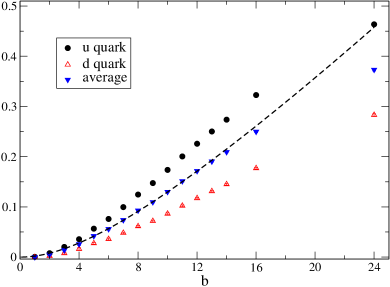
Figure 6: Relative increment of the quark condensate as a function of the magnetic field. We report separately data for the $u$ and $d$ quarks as well as for the average of the two, together with our best fit reported in the 6th line of Table 3.

$b_{\rm min}$	$b_{\rm max}$	$\chi^{2}/\textnormal{ndf}$	$m_{\pi}\;(MeV)$	$F_{\pi}\;(MeV)$
1	8	0.63	457(59)	54.7(5.6)
1	9	0.93	392(39)	61.7(4.2)
1	10	0.89	374(27)	63.8(2.9)
1	11	0.80	369(20)	64.3(2.1)
1	12	0.79	359(15)	65.6(1.6)
1	13	0.97	344(14)	67.2(1.4)
1	14	1.40	328(14)	69.1(1.4)
1	16	1.92	310(13)	71.1(1.3)
1	24	17.4	227(22)	80.8(2.3)
4	14	1.00	320(12)	69.9(1.2)
6	14	0.97	313(13)	70.6(1.3)
8	14	0.83	298(15)	72.2(1.5)

Table 3: Results from a fit of our data to Eq. (29). The notation for $b_{\rm min}$ and $b_{\rm max}$ is as in Table 2.

$b_{\rm min}$	$b_{\rm max}$	$\chi^{2}/\textnormal{ndf}$	$\Lambda_{B}\;(MeV)$	$\nu$
1	4	0.23	784(54)	2.33(19)
1	5	0.19	817(25)	2.23(9)
1	6	0.84	900(42)	2.00(12)
1	7	0.92	940(31)	1.90(8)
1	8	0.97	965(24)	1.85(6)
1	9	1.7	1006(26)	1.75(6)
1	10	1.9	1031(21)	1.70(5)
1	11	1.9	1045(18)	1.67(4)
1	12	2.3	1064(15)	1.63(4)
1	13	3.1	1083(15)	1.59(4)
1	14	4.3	1104(16)	1.55(4)
1	16	6.4	1131(16)	1.50(4)
1	24	35.8	1254(30)	1.29(5)

Table 4: Results from a fit $r(B)=(|e|B/\Lambda_{B}^{2})^{\nu}$. The notation for $b_{\rm min}$ and $b_{\rm max}$ is as in Table 2.

We have then tried to fit our data with the prediction of Ref. Cohen:2007bt , as reported in Eq. (29). We have obtained reasonable fits only if both $m_{\pi}$ and $F_{\pi}$ are treated as independent free parameters, results are reported in Table 3. Data are well described by the prediction in Eq. (29) over a wide range of values of $|e|B$, including $b=14$ (i.e. $|e|B\sim$ 700 MeV), even if the fitted values of $F_{\pi}$ and $m_{\pi}$ are not very stable as the range is modified.

Typical values of the fit parameters are $m_{\pi}\sim 300-400$ MeV and $F_{\pi}\sim 60-70$ MeV. The fitted pion mass is somewhat larger than the value obtained, with the same discretization settings, by measuring meson correlators, i.e. $m_{\pi}\sim 200$ MeV demusa , however that is quite reasonable if we take into account the many discretization systematic effects which affect our simulations. The most relevant comes from the explicit flavour symmetry breaking induced by the staggered discretization: the three pions are not degenerate in mass and what is determined by meson correlator measurements is just the lowest pion mass: it is therefore likely that the $\chi$PT prediction still holds, but with an heavier effective pion mass.

Regarding $F_{\pi}$, the fitted values are about $\sim$ 20-30% lower than the expected physical value, $F_{\pi}\simeq 93$ MeV. We notice that $F_{\pi}$ enters Eq. (29) only in the prefactor, hence its value is surely affected by the systematic uncertainty in the overall normalization factor for $r(B)$, which is of the order of 10%. There are also corrections expected from the fact that we are not at zero temperature: the authors of Ref. Agasian:2001ym predict $F_{\pi}^{2}(T)\simeq F_{\pi}^{2}-{T^{2}}/{6}$, however in our case $T\simeq 40$ MeV and that can account for at most a 2% discrepancy from the physical value. The non-physical large value of $m_{\pi}$ can also affect $F_{\pi}$, but $\chi$PT would predict an increased value of $F_{\pi}$ chipt .

There are however many other possible sources of systematic uncertainties, including the fact that the $\chi$PT prediction of Ref. Cohen:2007bt has been obtained in the low energy limit $|e|B\ll\Lambda_{\rm QCD}^{2}$, a condition which is violated in our explored range of fields. We have verified that other two-parameter functions, which allow to fix independently the curvature at $B=0$ and the asymptotic linear behavior for larger fields (like Eq. (29) when $F_{\pi}$ and $m_{\pi}$ are treated as independent parameters) work equally well. For instance the function

$$r(b)=c_{0}b\ {\rm atan}(c_{1}b)$$ (32)

fits well in the whole range of explored fields, $b_{\rm min}=1$ and $b_{\rm max}=16$, with $c_{0}=0.0136(2)$, $c_{1}=0.140(5)$ and $\chi^{2}/{\rm d.o.f.}\simeq 0.77$.

To compare with the analysis performed in Ref. itep2 , we have also investigated if a power law behaviour $r(B)=(|e|B/\Lambda_{B}^{2})^{\nu}$ can fit our data. Results are reported in Table 4. Reasonable fits are obtained only for a range of fields including $b=8$. That coincides more or less with the range for which also the quadratic fit works well, and indeed values obtained for $\nu$ in this range are roughly compatible with $\nu=2$.

We are not able to say much about the strong field regime, $|e|B\gg\Lambda_{\rm QCD}^{2}$, since saturation effects make such regime unaccessible to our present investigation: much smaller lattice spacings should be used to that aim.

III.4 Density of zero modes

Let us finally discuss our results for the densities of zero modes of the Dirac operator, $\rho_{u}(0)$ and $\rho_{d}(0)$, obtained for the $u$ and $d$ quarks respectively. We have determined such densities following Eq. (20), i.e. determining on our ensemble of configurations, sampled with a dynamical quark mass $am=0.01335$, the average of ${\rm Tr}(M^{-1}(am^{\prime}))$ for various different values of $m^{\prime}$ and then extrapolating to $am^{\prime}=0$. In particular we have chosen $am^{\prime}=0.007,0.01335,0.02$ and $0.03$. A quadratic extrapolation in $m^{\prime}$ works well in all cases.

In Table 5 we report data for the relative increments $\tilde{r}_{u}$ and $\tilde{r}_{d}$ of $\rho_{u}(0)$ and $\rho_{d}(0)$ as a function of $B$, also for the cases in which only the valence or the dynamical contributions are taken into account; the average quantities are plotted in Fig. 7. We notice, comparing Table 5 with Table 1, that the relative increment of the zero mode density, $\tilde{r}$, is generally larger than the corresponding increment in the condensate, $r$. Moreover Fig. 7 shows that, similarly to what happens for the condensate, it is possible to make a separation of the total increment into a valence and a dynamical contribution, which sum approximately to the total increment. Also in this case the change in the distribution of the non-Abelian gauge fields (dynamical contribution) accounts for about 30-40% of the total increase.

$b$	$\tilde{r}_{u}(b)$	$\tilde{r}_{d}(b)$	$\tilde{r}^{val}_{u}(b)$	$\tilde{r}^{val}_{d}(b)$	$\tilde{r}^{dyn}_{u/d}(b)$
1	0.003(4)	0.000(4)	0.002(3)	0.002(3)	0.002(3)
2	0.013(4)	0.002(5)	0.007(3)	0.003(3)	0.003(3)
3	0.026(4)	0.014(5)	0.022(4)	0.007(4)	0.009(4)
4	0.042(3)	0.024(4)	0.034(4)	0.010(5)	0.012(4)
5	0.069(3)	0.034(5)	0.047(3)	0.016(3)	0.018(3)
6	0.080(3)	0.040(7)	0.068(3)	0.021(4)	0.027(4)
7	0.117(3)	0.062(4)	0.087(3)	0.031(4)	0.036(3)
8	0.144(5)	0.076(5)	0.113(6)	0.037(5)	0.045(5)
9	0.173(5)	0.088(4)	0.138(5)	0.044(4)	0.050(3)
10	0.201(3)	0.101(7)	0.158(5)	0.052(5)	0.056(3)
11	0.236(5)	0.124(4)	0.185(5)	0.063(5)	0.069(4)
12	0.264(4)	0.142(5)	0.207(4)	0.074(5)	0.076(3)
14	0.319(5)	0.178(8)	0.256(4)	0.091(4)	0.097(3)
16	0.372(5)	0.211(5)	0.302(6)	0.115(4)	0.110(3)

Table 5: Relative increment of the density of zero modes of the Dirac operator for the $u$ and $d$ quarks and for various magnetic field values. We report full data, as well as valence and dynamical contributions separately.

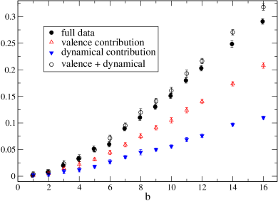
Figure 7: Relative increment of the average of the $\rho_{u}(0)$ and $\rho_{d}(0)$ as a function of the magnetic field. We report separately $\tilde{r}(B),\tilde{r}^{val}(B),\tilde{r}^{dyn}(B)$ and $\tilde{r}^{val}(B)+\tilde{r}^{dyn}(B)$.

IV Conclusions

In this study we have approached the issue of magnetic catalysis by numerical lattice simulation of $N_{f}=2$ QCD. We have adopted a rooted standard staggered discretization of the fermion action and a plaquette pure gauge action on a symmetric $16^{4}$ lattice, corresponding to a lattice spacing $a\simeq 0.3$ fm, a (Goldstone) pion mass $m_{\pi}\simeq 200$ MeV and a temperature well below the deconfinement/chiral restoring one ($T\sim 40$ MeV). We have studied the breaking of chiral symmetry as a function of a constant and uniform magnetic field directed along the $\hat{z}$ axis. Explored magnetic fields, allowed by the toroidal geometry and for which distortion (saturation) effects due to the lattice discretization are not significant, range from $|e|B\sim(180\ {\rm MeV})^{2}$ to $|e|B\sim(700\ {\rm MeV})^{2}$.

We have shown that, in the range of explored fields, it is possible to divide magnetic catalysis into a contribution coming from the modified distribution of non-Abelian gauge fields, induced by dynamical quark loop effects, that we have called dynamical contribution, and a valence contribution, determined by measuring the condensate on gauge configurations sampled with the unmodified distribution. The first term, which is missed by quenched or partially quenched studies, accounts for about 40% of the total increase in the quark condensate. Results obtained for the density of zero modes looks quite similar.

Regarding the dependence of the condensate on the magnetic field, we have shown that a quadratic behavior, which is expected in the limit of small magnetic fields, describes well our data for $|e|B$ up to $\sim$ (500 MeV)². The $\chi$PT prediction of Ref. Cohen:2007bt fits data over a wider range, but only if the pion decay constant is treated as an independent free parameter.

Our investigation can be improved in several respects. Lattice artifacts may affect our results in various different ways, ranging from the presence of a distorted meson spectrum in the adopted rooted staggered fermion formulation, to residual renormalization effects and possible residual saturation effects in the explored range of fields. An improved lattice formulation and a finer spacing $a$ would allow to check for such artifacts, to test the correct scaling to the continuum limit of our results and to explore larger values of the magnetic field. A larger spatial volume would instead allow for a finer quantization of $|e|B$ and a better investigation of the small field region. It would be also interesting to explore different choices of the quark mass spectrum, in order to see how the separation of magnetic catalysis into a dynamical and a valence contribution depends on the dynamical quark masses. We plan to address such issues in future studies.

- (1) T. Vachaspati, Phys. Lett. B 265, 258 (1991).
- (2) D. E. Kharzeev, L. D. McLerran and H. J. Warringa, Nucl. Phys. A 803, 227 (2008).
- (3) V. Skokov, A. Y. Illarionov and V. Toneev, Int. J. Mod. Phys. A 24, 5925 (2009).
- (4) D. E. Kharzeev, L. D. McLerran and H. J. Warringa, Nucl. Phys. A 803, 227 (2008).
- (5) K. Fukushima, D. E. Kharzeev and H. J. Warringa, Phys. Rev. D 78, 074033 (2008).
- (6) B. I. Abelev et al. [STAR Collaboration], Phys. Rev. Lett. 103, 251601 (2009).
- (7) R. C. Duncan and C. Thompson, Astrophys. J. 392, L9 (1992).
- (8) S. Mereghetti, Astron. Astrophys. Rev. 15, 225-287 (2008). [arXiv:0804.0250 [astro-ph]].
- (9) A. Salam and J. A. Strathdee, Nucl. Phys. B 90, 203 (1975).
- (10) A. D. Linde, Phys. Lett. B 62, 435 (1976).
- (11) S. Kawati, G. Konisi, H. Miyata, Phys. Rev. D28, 1537-1541 (1983).
- (12) S. P. Klevansky and R. H. Lemmer, Phys. Rev. D 39, 3478 (1989).
- (13) H. Suganuma and T. Tatsumi, Annals Phys. 208, 470 (1991).
- (14) K. G. Klimenko, Z. Phys. C 54, 323 (1992).
- (15) S. Schramm, B. Muller, A. J. Schramm, Mod. Phys. Lett. A7, 973-982 (1992).
- (16) K. G. Klimenko, B. V. Magnitsky, A. S. Vshivtsev, Nuovo Cim. A107, 439-452 (1994).
- (17) V. P. Gusynin, V. A. Miransky and I. A. Shovkovy, Phys. Rev. Lett. 73, 3499 (1994) [Erratum-ibid. 76, 1005 (1996)] [arXiv:hep-ph/9405262].
- (18) V. P. Gusynin, V. A. Miransky and I. A. Shovkovy, Phys. Lett. B 349, 477 (1995).
- (19) I. A. Shushpanov and A. V. Smilga, Phys. Lett. B 402, 351 (1997).
- (20) A. Y. .Babansky, E. V. Gorbar, G. V. Shchepanyuk, Phys. Lett. B419, 272-278 (1998). [hep-th/9705218].
- (21) D. Ebert, K. G. Klimenko, M. A. Vdovichenko and A. S. Vshivtsev, Phys. Rev. D 61, 025005 (2000).
- (22) A. Goyal, M. Dahiya, Phys. Rev. D62, 025022 (2000). [hep-ph/9906367].
- (23) N. O. Agasian and I. A. Shushpanov, Phys. Lett. B 472, 143 (2000) [arXiv:hep-ph/9911254].
- (24) D. Ebert, V. V. Khudyakov, V. C. Zhukovsky, K. G. Klimenko, Phys. Rev. D65, 054024 (2002). [hep-ph/0106110].
- (25) D. N. Kabat, K. -M. Lee, E. J. Weinberg, Phys. Rev. D66, 014004 (2002). [hep-ph/0204120].
- (26) V. A. Miransky and I. A. Shovkovy, Phys. Rev. D 66, 045006 (2002).
- (27) T. D. Cohen, D. A. McGady and E. S. Werbos, Phys. Rev. C 76, 055201 (2007).
- (28) C. V. Johnson and A. Kundu, JHEP 0812, 053 (2008) [arXiv:0803.0038 [hep-th]].
- (29) E. Rojas, A. Ayala, A. Bashir, A. Raya, Phys. Rev. D77, 093004 (2008). [arXiv:0803.4173 [hep-ph]].
- (30) O. Bergman, G. Lifschytz and M. Lippert, Phys. Rev. D 79, 105024 (2009) [arXiv:0806.0366 [hep-th]].
- (31) A. V. Zayakin, JHEP 0807, 116 (2008).
- (32) N. Evans, T. Kalaydzhyan, K. y. Kim and I. Kirsch, JHEP 1101, 050 (2011) [arXiv:1011.2519 [hep-th]].
- (33) A. J. Mizher, E. S. Fraga, M. N. Chernodub, [arXiv:1103.0954 [hep-ph]].
- (34) S. -i. Nam, C. -W. Kao, [arXiv:1103.6057 [hep-ph]].
- (35) N. O. Agasian and S. M. Fedorov, Phys. Lett. B 663, 445 (2008).
- (36) E. S. Fraga and A. J. Mizher, Phys. Rev. D 78, 025016 (2008);
- (37) D. P. Menezes, M. Benghi Pinto, S. S. Avancini, A. Perez Martinez, C. Providencia, Phys. Rev. C79, 035807 (2009). [arXiv:0811.3361 [nucl-th]].
- (38) A. Ayala, A. Bashir, A. Raya, A. Sanchez, Phys. Rev. D80, 036005 (2009). [arXiv:0904.4533 [hep-ph]].
- (39) J. K. Boomsma and D. Boer, Phys. Rev. D 81, 074005 (2010).
- (40) K. Fukushima, M. Ruggieri and R. Gatto, arXiv:1003.0047 [hep-ph].
- (41) A. J. Mizher, M. N. Chernodub, E. S. Fraga, Phys. Rev. D82, 105016 (2010). [arXiv:1004.2712 [hep-ph]].
- (42) M. D’Elia, S. Mukherjee, F. Sanfilippo, Phys. Rev. D82, 051501 (2010). [arXiv:1005.5365 [hep-lat]].
- (43) R. Gatto, M. Ruggieri, Phys. Rev. D82, 054027 (2010). [arXiv:1007.0790 [hep-ph]].
- (44) I. E. Frolov, V. C. .Zhukovsky, K. G. Klimenko, Phys. Rev. D82, 076002 (2010). [arXiv:1007.2984 [hep-ph]].
- (45) S. .Fayazbakhsh, N. Sadooghi, Phys. Rev. D83, 025026 (2011). [arXiv:1009.6125 [hep-ph]].
- (46) R. Gatto, M. Ruggieri, Phys. Rev. D83, 034016 (2011). [arXiv:1012.1291 [hep-ph]].
- (47) F. Preis, A. Rebhan, A. Schmitt, [arXiv:1012.4785 [hep-th]].
- (48) P. Cea and L. Cosmai, JHEP 0508, 079 (2005).
- (49) P. Cea, L. Cosmai and M. D’Elia, JHEP 0712, 097 (2007).
- (50) M. N. Chernodub, Phys. Rev. D82, 085011 (2010). [arXiv:1008.1055 [hep-ph]].
- (51) M. N. Chernodub, [arXiv:1101.0117 [hep-ph]].
- (52) N. Callebaut, D. Dudal, H. Verschelde, [arXiv:1102.3103 [hep-ph]].
- (53) P. V. Buividovich, M. N. Chernodub, E. V. Luschevskaya and M. I. Polikarpov, Phys. Lett. B 682, 484 (2010), Nucl. Phys. B 826, 313 (2010).
- (54) V. V. Braguta, P. V. Buividovich, T. Kalaydzhyan, S. V. Kuznetsov, M. I. Polikarpov, PoS LATTICE2010, 190 (2010). [arXiv:1011.3795 [hep-lat]].
- (55) T. Banks, A. Casher, Nucl. Phys. B169, 103 (1980).
- (56) P. V. Buividovich, M. N. Chernodub, E. V. Luschevskaya and M. I. Polikarpov, Phys. Rev. D 80, 054503 (2009).
- (57) M. Abramczyk, T. Blum, G. Petropoulos and R. Zhou, arXiv:0911.1348 [hep-lat].
- (58) P. V. Buividovich, M. N. Chernodub, D. E. Kharzeev, T. Kalaydzhyan, E. V. Luschevskaya and M. I. Polikarpov, arXiv:1003.2180 [hep-lat].
- (59) M. H. Al-Hashimi and U. J. Wiese, Annals Phys. 324, 343 (2009).
- (60) S. Ejiri et al., Phys. Rev. D 80, 094505 (2009) [arXiv:0909.5122 [hep-lat]].
- (61) D.J. Wallace and R.K.P. Zia, Phys. Rev. B 12, 5340 (1975).
- (62) P. Hasenfratz and H. Leutwyler, Nucl. Phys. B 343, 241 (1990),
- (63) A. V. Smilga, Phys. Lett. B 318, 531 (1993); A. V. Smilga and J. J. M. Verbaarschot, Phys. Rev. D 54, 1087 (1996).
- (64) N. O. Agasian, I. A. Shushpanov, JHEP 0110, 006 (2001). [hep-ph/0107128].
- (65) J. Gasser, H. Leutwyler, Annals Phys. 158, 142 (1984); Nucl. Phys. B250 (1985) 465.