Bethe-Salpeter approach to the collective-mode spectrum of a superfluid Fermi gas in a moving optical lattice

Abstract

We have derived the Bethe-Salpeter (BS) equations for the collective-mode spectrum of a mixture of fermion atoms of two hyperfine states loaded into a moving optical lattice. The collective excitation spectrum exhibits rotonlike minimum and the Landau instability takes place when the energy of the rotonlike minimum hits zero. The BS approach is compared with the other existing methods for calculating the collective-mode spectrum. In particular, it is shown that the spectrum obtained by the BS equations in an excellent agreement with corresponding spectrum obtained by the perturbation theory, while the Green’s function formalism provides slightly different results for the collective excitations.

I Introduction

Ultracold atoms loaded in optical lattices are ideal systems to simulate and study many different problems of correlated quantum systems because near the Feshbach resonance the atom-atom interaction can be manipulated in a controllable way by changing the scattering length $a_{s}$ from the Bardeen-Cooper-Schrieffer (BCS) side (negative values) to the BEC side (positive values) reaching very large values close to resonance. On Bose-Einstein condensation (BEC) side of the resonance the spin-up and spin-down atoms can form diatomic molecules, and these bosonic molecules can undergo a BEC at low enough temperature. BEC1 ; BEC2 ; BEC3 ; BEC4 We focus our attention on the BCS side where BCS superfluidity is expected analogous to superconductivity.

In what follows we examine the spectrum of the single-particle excitations and the spectrum of the collective excitations of a balanced mixture of atomic Fermi gas of two hyperfine states with contact interaction loaded into an optical lattice. The two hyperfine states are described by pseudospins $\sigma=\uparrow,\downarrow$. There are $M$ atoms distributed along $N$ sites, and the corresponding filling factors $f=M/N$ are assumed to be smaller than unity. If the lattice potential is sufficiently deep such that the tight-binding approximation is valid, the system is well described by the single-band attractive Hubbard model:

$$H=-J\sum_{<i,j>,\sigma}\psi^{\dagger}_{i,\sigma}\psi_{j,\sigma}-\mu\sum_{i,\sigma}\widehat{n}_{i,\sigma}+U\sum_{i}\widehat{n}_{i,\uparrow}\widehat{n}_{i,\downarrow}.$$ (1)

Here, the Fermi operator $\psi^{\dagger}_{i,\sigma}$ ($\psi_{i,\sigma}$) creates (destroys) a fermion on the lattice site $i$ with pseudospin $\sigma$ and $\widehat{n}_{i,\sigma}=\psi^{\dagger}_{i,\sigma}\psi_{i,\sigma}$ is the density operator on site $i$ with a position vector $\textbf{r}_{i}$. $\mu$ is the corresponding chemical potential, and the symbol $\sum_{<ij>}$ means sum over nearest-neighbor sites. $J$ is the tunneling strength of the atoms between nearest-neighbor sites, and $U$ is the on-site interaction. On the BCS side the interaction parameter $U$ is negative (the atomic interaction is attractive). We assume $\hbar=1$, Boltzmann constant $k_{B}=1$, $J=1$ and the lattice constant $a=1$.

In the case when the periodic array of microtraps is generated by counter propagating laser beams with different frequencies the optical lattice potential is moving with a velocity $-\textbf{v}$ (in the laboratory frame) which magnitude is proportional to the relative frequency detuning of the two laser beams. In a frame fixed with respect to the lattice potential the fermion atoms flows with a constant quasimomentum $\textbf{p}=m\textbf{v}$, where $m$ is the mass of the loaded atoms. For balance Fermi gases the order parameter field $\Phi_{j}(u)=-|U|<\psi_{j,\downarrow}(u)\psi_{j,\uparrow}(u)>$ (or $\Phi^{*}_{j}(u)=-|U|<\psi^{\dagger}_{j,\uparrow}(u)\psi^{\dagger}_{j,\downarrow}(u)>$) in the mean-field approximation varies as $\Phi_{j}\propto\Delta_{0}\exp\left[2\imath\textbf{p.}\textbf{r}_{j}\right]$. Here, the symbol $<>$ means ensemble average, and $\Delta$ is a real quantity which depends on the lattice velocity.Gam ; Yosh In a moving lattice the formation of a BCS superfluidity is possible, but due to the presence of quasimomentum p the superflow can break down. The stability of balance superfluid Fermi gases loaded into a moving optical lattice has been recently studied using the second-order time-dependent perturbation theory Gam , and the Green’s function formalism. Yosh The superfluid state could be destabilized at a critical flow momentum via two different mechanisms: depairing (pair-breaking) at $\textbf{p}_{pb}$ and Landau instabilities at $\textbf{p}_{cr}$. The depairing takes place when the single fermionic excitations are broken, while the Landau instability is related to the rotonlike structure of the spectrum of the collective excitations. The superfluid state becomes unstable when the energy of the rotonlike minimum reaches zero at a given quasimomentum. The numerical solution of the number, gap and the collective-mode equations shows that at a zero temperature the Landau instability appears before the depearing mechanism.Yosh

Generally speaking, there exist three methods that can be used to calculate the spectrum of the collective excitations of Hamiltonian (1) in a stationary (or moving) optical lattice in generalized random phase approximation (GRPA). The first approach uses the Green’s function method,CGexc ; CCexc ; CG1 ; ZKexc ; Com ; ZGK ; ZK1 the second one is based on the Anderson-Rickayzen equations,PA ; R ; BR while the third employs the perturbation technique.Gam

Decades ago, the Green’s function approach has been used to obtain the collective excitations in the exciton problem CGexc ; CCexc and in the s-wave layered superconductors. CG1 In both cases we have deal with a system of interacting electrons, where two different interactions exist: the Coulomb interaction $v(\textbf{r})=e^{2}/|\textbf{r}|$ and a short-range attractive interaction $g(\textbf{r})$ between electrons. In the GRPA the collective-mode spectrum can be obtained by the poles of: (i) the vertex $\Gamma$ from the corresponding BS equation for $\Gamma$, CCexc ; Com (ii) the two-particle Green’s function $K$ by solving the BS equation for the BS amplitudes, ZKexc ; ZGK ; ZK1 and (iii) the density and spin response functions.CGexc ; CG1 It is worth mentioning that in the exciton problem the BS vertex equation CCexc and the BS equation $K^{-1}=K^{(0)-1}-I_{d}-I_{exc}$ (here $K^{(0)}$ is the free two-particle propagator, and $I_{d}$ takes into account the direct interaction between the electrons, while $I_{exc}$ describes their exchange interactionZKexc ), both provide the same collective-mode spectrum, while in the case of superconductivity, the vertex equation obtained in Ref. [Com, ] in for the collective-mode dispersion (see Eq. (14) in Ref. [Com, ]) is incorrect because the exchange interaction has been neglected (the incorrect equation follows from our secular determinant (9) assuming a stationary lattice and neglecting all elements with $\widetilde{\gamma}$ and $m$ indices).

Côté and Griffin CGexc ; CG1 have obtained the collective excitation spectrum from the poles of the density and spin response functions using the Baym and Kadanoff formalism. BK They have ignored the long-range Coulomb interaction keeping in the direct interaction only the ladder diagrams involving the short-range interaction. The exchange interaction involves bubble diagrams with respect to both the unscreened Coulomb interaction $v(\textbf{r})$ and the short-range attractive interaction $g(\textbf{r})$. Thus, Eq. (2.33) in Ref. [CG1, ] corresponds to the BS equation $\widetilde{K}^{-1}=K^{(0)-1}-I_{d}$, and Eq. (2.32) in Ref. [CG1, ] corresponds to the BS equation $K=\widetilde{K}+\widetilde{K}I_{exc}K$. The Côté and Griffin Green’s function formalism was employed in Ref. [Yosh, ] to study the collective-mode spectrum in moving optical lattices by obtaining the poles of the density response function. In what follows we will see that the BS approach provides collective-mode spectrum which lies slightly below the one obtained in Ref. [Yosh, ] if the both methods use the same gap and chemical potential. The most important advantage of the BS formalism over the Green s function approach is that within the BS approach we can obtain the poles of density and spin response functions in a uniform manner, i.e. one secular determinant provides not only the poles of the density response function, but the poles of the spin response function as well.

The second method BR that can be used to obtain the collective excitation spectrum of Hamiltonian (1) starts from the Anderson-Rickayzen equations, which in the GRPA were reduced to a set of three coupled equations and the collective-mode spectrum is obtained by solving the secular equation $Det|A|=0$, where

$$A=\left(\begin{array}[]{ccc}|U|^{-1}+I_{l,l}&J_{\gamma,l}&I_{l,m}\\ I_{\gamma,l}&|U|^{-1}+I_{\gamma,\gamma}&J_{\gamma,m}\\ I_{l,m}&J_{\gamma,m}&|U|^{-1}+I_{m,m}\end{array}\right).$$ (2)

In a stationary lattice, the quantities $I$ and $J$ are defined in Sec. II by Eqs. (10) when $\textbf{p}=0$. As can be seen, the BS secular determinant provides an equation for the collective-mode dispersion that depends on all four coherence factors and the associated determinant is $4\times 4$, while the determinant (2) does not depend on the fourth coherence factor $\widetilde{\gamma}$, so that the corresponding determinant is only $3\times 3$.

Recently, Ganesh et al.Gam have used a perturbation approach which in the case of a moving optical lattice provides the following $3\times 3$ secular determinant (see Eqs. (B8) in Ref. [Gam, ], where there is a negative sign in front of the sum in the definition of $\chi_{0}^{2,3}$):

$$D=\left(\begin{array}[]{ccc}|U|^{-1}+I^{\textbf{p}}_{m,m}&(J^{\textbf{p}}_{\gamma,m}-I^{\textbf{p}}_{lm})/2&-(J^{\textbf{p}}_{\gamma,m}+I^{\textbf{p}}_{l,m})/2\\ I^{\textbf{p}}_{l,m}-J^{\textbf{p}}_{\gamma,m}&|U|^{-1}+(I^{\textbf{q}}_{l,l}+I^{\textbf{p}}_{\gamma,\gamma}-2J^{\textbf{p}}_{\gamma,l})/2&(I^{\textbf{p}}_{\gamma,\gamma}-I^{\textbf{p}}_{l,l})/2\\ -I^{\textbf{p}}_{l,m}-J^{\textbf{p}}_{\gamma,m}&(I^{\textbf{p}}_{\gamma,\gamma}-I^{\textbf{p}}_{l,l})/2&|U|^{-1}+(I^{\textbf{p}}_{l,l}+I^{\textbf{p}}_{\gamma,\gamma}+2J^{\textbf{p}}_{\gamma,l})/2\end{array}\right).$$ (3)

Since $Det|D|=det|A^{\textbf{p}}|$, where

$$A^{\textbf{p}}=\left|\begin{array}[]{cccc}|U|^{-1}+I^{\textbf{p}}_{\gamma,\gamma}&J^{\textbf{p}}_{\gamma,l}&J^{\textbf{p}}_{\gamma,m}\\ J^{\textbf{p}}_{\gamma,l}&|U|^{-1}+I^{\textbf{p}}_{l,l}&I^{\textbf{p}}_{l,m}\\ J^{\textbf{p}}_{\gamma,m}&I^{\textbf{p}}_{l,m}&|U|^{-1}+I^{\textbf{p}}_{m,m}\end{array}\right|,$$ (4)

one can say that the perturbation method is a generalization of the Belkhir and Randeria method to the case of moving optical lattice.

This paper is organized as follows. In Sec. II, we derive the BS equations for the dispersion of the collective excitations of imbalanced mixture of fermionic atoms loaded in a moving optical lattice. In Sec. III, we compare our approach with the other existing methods, and we discuss the stability of balance gases loaded in a moving lattice. It turns out that the BS approach and the second-order time-dependent perturbation theoryGam provide essentially the same spectrum of the collective excitations, while the spectrum obtained by the Green’s function methodYosh differs from the corresponding dispersion obtained by the BS approach. But, the Green’s function method and the BS approach, both predict that as the quasimomentum p increases, the rotonlike minimum reaches zero before the pair-breaking mechanism takes place.

II Bethe-Salpeter equation for the spectrum of the collective modes

A basic approximation in our approach is that the single-particle excitations in the system will be calculated in the mean-field approximation, i.e. our single-particle Green’s function in the momentum and frequency space is the following $2\times 2$ matrix $\widehat{G}=\left(\begin{array}[]{cc}G^{\uparrow,\uparrow}&G^{\uparrow,\downarrow}\\ G^{\downarrow,\uparrow}&G^{\downarrow,\downarrow}\end{array}\right)$. The the corresponding matrix elements are defined as follows:

$$G^{ij}_{\textbf{p}}(\textbf{k},\imath\omega_{m})=\frac{A^{ij}_{\textbf{p}}(\textbf{k})}{\imath\omega_{m}-E_{+}(\textbf{k};\textbf{p})}+\frac{B^{ij}_{\textbf{p}}(\textbf{k})}{\imath\omega_{m}-E_{-}(\textbf{k};\textbf{p})},$$

where

$$\begin{split}&\widehat{A}_{\textbf{p}}(\textbf{k})=\left(\begin{array}[]{cc}u^{2}_{\textbf{p}}(\textbf{k})&u_{\textbf{p}}(\textbf{k})v_{\textbf{p}}(\textbf{k})\\ u_{\textbf{p}}(\textbf{k})v_{\textbf{p}}(\textbf{k})&v^{2}_{\textbf{p}}(\textbf{k})\end{array}\right)\\ &\widehat{B}_{\textbf{p}}(\textbf{k})=\left(\begin{array}[]{cc}v^{2}_{\textbf{p}}(\textbf{k})&-u_{\textbf{p}}(\textbf{k})v_{\textbf{p}}(\textbf{k})\\ -u_{\textbf{p}}(\textbf{k})v_{\textbf{p}}(\textbf{k})&u^{2}_{\textbf{p}}(\textbf{k})\end{array}\right).\end{split}$$

The symbol $\omega_{m}$ denotes $\omega_{m}=(2\pi/\beta)(m+1/2);\beta=T^{-1}$, $T$ is the temperature, and $m=0,\pm 1,\pm 2,...$. Here, $u_{\textbf{p}}(\textbf{k})=\sqrt{\frac{1}{2}\left[1+\chi(\textbf{k};\textbf{p})/E_{\textbf{p}}(\textbf{k})\right]}$ and $v_{\textbf{p}}(\textbf{k})=\sqrt{\frac{1}{2}\left[1-\chi(\textbf{k};\textbf{p})/E_{\textbf{p}}(\textbf{k})\right]}$ are the coherent factors, and we have introduced the following notations $\chi(\textbf{k};\textbf{p})=\frac{1}{2}\left[\xi(\textbf{p}+\textbf{k})+\xi(\textbf{k}-\textbf{p})\right]$, $\eta(\textbf{k};\textbf{p})=\frac{1}{2}\left[\xi(\textbf{p}+\textbf{k})-\xi(\textbf{k}-\textbf{p})\right]$, $E_{\pm}(\textbf{k};\textbf{p})=\eta(\textbf{k};\textbf{p})\pm E_{\textbf{p}}(\textbf{k})$, and $E_{\textbf{p}}(\textbf{k})=\sqrt{\chi^{2}(\textbf{k};\textbf{p})+\Delta^{2}}$. The tight-binding form of the electron energy is $\xi(\textbf{k})=2J\left(1-\sum_{\nu}\cos k_{\nu}\right)-\mu$. As can be seen, the single-particle excitations in the mean-field approximation are coherent combinations of electronlike $E_{+}$ and holelike $E_{-}$ fermionic excitations.

The thermodynamic potential in a mean-field approximation can be evaluated as a summation of quasiparticles with energy $E_{\pm}(\textbf{k})$:

$$\begin{split}&\Omega=\frac{\Delta^{2}}{|U|}+\frac{1}{N}\sum_{\textbf{k}}\{\chi(\textbf{k};\textbf{p})-E_{\textbf{p}}(\textbf{k})\\ &-\frac{1}{\beta}\ln\left(\left[1+\exp\left(-\beta E_{+}(\textbf{k};\textbf{p})\right)\right]\left[1+\exp\left(\beta E_{-}(\textbf{k};\textbf{p})\right)\right]\right)\}.\end{split}$$

In the case of balance population of fermionic atoms the gap and particle number equations can be obtained by minimizing the free energy $F(\Delta,f)=\Omega+\mu f$ with respect to $\mu$ and $\Delta$:

$$\begin{split}&f=\frac{2}{N}\sum_{\textbf{k}}\left[u_{\textbf{p}}^{2}(\textbf{k})f(E_{+}(\textbf{k};\textbf{p})+v_{\textbf{p}}^{2}(\textbf{k})f(E_{-}(\textbf{k};\textbf{p})\right],\\ &1=\frac{|U|}{N}\sum_{\textbf{k}}\frac{f(E_{-}(\textbf{k};\textbf{p}))-f(E_{+}(\textbf{k};\textbf{p}))}{2E_{\textbf{p}}(\textbf{k})},\end{split}$$ (5)

where $f(x)=\left[\exp\left(\beta x\right)+1\right]^{-1}$ is the Fermi distribution function.

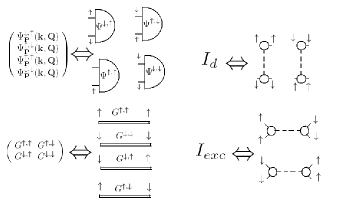
Figure 1: Diagrammatic representation of the Bethe-Salpeter amplitude, the single-particle Green’s function, the direct and exchange interactions.

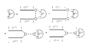
Figure 2: Diagrammatic representation of the Bethe-Salpeter equation for the amplitude $\Psi_{\textbf{p}}^{\downarrow,\uparrow}(\textbf{k},\textbf{Q})$.

Next, we derive the BS equations for the spectrum of the collective modes in a moving lattice. The collective mode energies $\omega_{\textbf{p}}(\textbf{Q})$ and the corresponding BS amplitude $\widehat{\Psi}_{\textbf{p}}(\textbf{k},\textbf{Q})=\left(\begin{array}[]{c}\Psi_{\textbf{p}}^{\downarrow,\uparrow}(\textbf{k},\textbf{Q})\\ \Psi_{\textbf{p}}^{\uparrow,\downarrow}(\textbf{k},\textbf{Q})\\ \Psi_{\textbf{p}}^{\uparrow,\uparrow}(\textbf{k},\textbf{Q})\\ \Psi_{\textbf{p}}^{\downarrow,\downarrow}(\textbf{k},\textbf{Q})\\ \end{array}\right)$ in a moving optical lattice and spin-polarized systems can be derived in a similar manner as in a stationary lattice. Our approach is based on the fact that the Hubbard model with on-site attractive interaction can be transformed to a model in which the narrow-band free electrons are coupled to a boson field due to some spin-dependent mechanism.ZGK ; ZK1 We first use the Hubbard-Stratonovich transformation to transform the quartic Hubbard term in (1) to a quadratic form. Thus, the quartic problem of interacting electrons is transformed to a quadratic problem of non-interacting Nambu fermion fields coupled to a Bose field and therefore, we arrive at the problem of the linear response of many-fermion systems under a weak bosonic field when a transition to a quantum condensed phase is possible. We have similar problem in exciton physics when the BEC of excitons can be described by applying the powerful arsenal of quantum field theory to obtain exact equations for the single-particle Green’s function, mass operator and the BS equation for the two-particle Green’s function.CGexc ; CCexc ; ZKexc As in the exciton problem, the mass operator is a sum of two terms: the Fock $\Sigma_{F}$ and Hartree $\Sigma_{H}$ terms. The Hartree term is diagonal with respect to the spin indices and it generates the exchange interaction $I_{exc}=\delta\Sigma_{H}/\delta G$ in the BS equation for the spectrum of the collective excitations, while the direct interaction $I_{d}=\delta\Sigma_{F}/\delta G$ in the kernel of the BS equation originates from the Fock term. In Fig. 1 we have shown the diagrammatic representations of the leading terms of the direct and exchange interactions. In this approximation the BS equation for the BS amplitude is $\Psi=K^{(0)}\left[I_{d}+I_{exc}\right]\Psi$, where $K^{(0)}$ is a product of two single-particle Green’s functions in the mean-field approximation. In Fig. 2 we have shown the BS equation for $\Psi_{\textbf{p}}^{\downarrow,\uparrow}(\textbf{k},\textbf{Q})$. The other three equations for $\Psi_{\textbf{p}}^{\uparrow,\downarrow}(\textbf{k},\textbf{Q})$, $\Psi_{\textbf{p}}^{\uparrow,\uparrow}(\textbf{k},\textbf{Q})$ and $\Psi_{\textbf{p}}^{\downarrow,\downarrow}(\textbf{k},\textbf{Q})$ are similar to that one. We can write all four BS equations as a single matrix equation:

$$\widehat{\Psi}_{\textbf{p}}(\textbf{k},\textbf{Q})=-\frac{|U|}{2N}\widehat{D}_{\textbf{p}}(\textbf{k},\textbf{Q},\imath\omega_{p})\sum_{\textbf{q}}\widehat{\Psi}_{\textbf{p}}(\textbf{q},\textbf{Q})+\frac{|U|}{2N}\widehat{M}_{\textbf{p}}(\textbf{k},\textbf{Q},\imath\omega_{p})\sum_{\textbf{q}}\widehat{\Psi}_{\textbf{p}}(\textbf{q},\textbf{Q}).$$ (6)

Here,

$$\widehat{D}=\left(\begin{array}[]{cccc}K_{\textbf{p}}^{\left(\downarrow,\downarrow,\uparrow,\uparrow\right)}(\textbf{k},\textbf{Q},\imath\omega_{p}),&K_{\textbf{p}}^{\left(\downarrow,\uparrow,\downarrow,\uparrow\right)}(\textbf{k},\textbf{Q},\imath\omega_{p})&0&0\\ K_{\textbf{p}}^{\left(\uparrow,\downarrow,\uparrow,\downarrow\right)}(\textbf{k},\textbf{Q},\imath\omega_{p}),&K_{\textbf{p}}^{\left(\uparrow,\uparrow,\downarrow,\downarrow\right)}(\textbf{k},\textbf{Q},\imath\omega_{p})&0&0\\ K_{\textbf{p}}^{\left(\uparrow,\downarrow,\uparrow,\uparrow\right)}(\textbf{k},\textbf{Q},\imath\omega_{p}),&K_{\textbf{p}}^{\left(\uparrow,\uparrow,\downarrow,\uparrow\right)}(\textbf{k},\textbf{Q},\imath\omega_{p})&0&0\\ K_{\textbf{p}}^{\left(\downarrow,\downarrow,\uparrow,\downarrow\right)}(\textbf{k},\textbf{Q},\imath\omega_{p}),&K_{\textbf{p}}^{\left(\downarrow,\uparrow,\downarrow,\downarrow\right)}(\textbf{k},\textbf{Q},\imath\omega_{p})&0&0\end{array}\right),\widehat{M}=\left(\begin{array}[]{cccc}0&0&K_{\textbf{p}}^{\left(\downarrow,\downarrow,\downarrow,\uparrow\right)}(\textbf{k},\textbf{Q},\imath\omega_{p}),&K_{\textbf{p}}^{\left(\downarrow,\uparrow,\uparrow,\uparrow\right)}(\textbf{k},\textbf{Q},\imath\omega_{p})\\ 0&0&K_{\textbf{p}}^{\left(\uparrow,\downarrow,\downarrow,\downarrow\right)}(\textbf{k},\textbf{Q},\imath\omega_{p}),&K_{\textbf{p}}^{\left(\uparrow,\uparrow,\uparrow,\downarrow\right)}(\textbf{k},\textbf{Q},\imath\omega_{p})\\ 0&0&K_{\textbf{p}}^{\left(\uparrow,\downarrow,\downarrow,\uparrow\right)}(\textbf{k},\textbf{Q},\imath\omega_{p}),&K_{\textbf{p}}^{\left(\uparrow,\uparrow,\uparrow,\uparrow\right)}(\textbf{k},\textbf{Q},\imath\omega_{p})\\ 0&0&K_{\textbf{p}}^{\left(\downarrow,\downarrow,\downarrow,\downarrow\right)}(\textbf{k},\textbf{Q},\imath\omega_{p}),&K_{\textbf{p}}^{\left(\downarrow,\uparrow,\uparrow,\downarrow\right)}(\textbf{k},\textbf{Q},\imath\omega_{p})\end{array}\right),$$

and the terms $|U|\widehat{D}=K^{(0)}I_{d}$ and $|U|\widehat{M}=K^{(0)}I_{exc}$ represent the contributions due to the direct and exchange interactions, respectively. The two-particle propagator $K_{\textbf{p}}^{\left(i,j,k,l\right)}(\textbf{k},\textbf{Q},\imath\omega_{p})$ is:

$$\begin{split}&K_{\textbf{p}}^{\left(i,j,k,l\right)}(\textbf{k},\textbf{Q},\imath\omega_{p}\rightarrow\omega+\imath 0^{+})=\sum_{\omega_{m}}G_{\textbf{p}}^{i,j}(\textbf{k}+\textbf{Q};\imath\omega_{p}+\imath\omega_{m})G_{\textbf{p}}^{k,l}(\textbf{k};\imath\omega_{m})|_{\imath\omega_{p}\rightarrow\omega+\imath 0^{+}}=\\ &\widetilde{A}^{ij}_{\textbf{p}}A^{kl}_{\textbf{p}}\frac{f(E_{+}(\textbf{k};\textbf{p}))-f(E_{+}(\textbf{k}+\textbf{Q};\textbf{p}))}{\omega-\left[E_{+}(\textbf{k}+\textbf{Q};\textbf{p})-E_{+}(\textbf{k};\textbf{p})\right]+\imath 0^{+}}+\widetilde{B}^{ij}_{\textbf{p}}B^{kl}_{\textbf{p}}\frac{f(E_{-}(\textbf{k};\textbf{p}))-f(E_{-}(\textbf{k}+\textbf{Q};\textbf{p}))}{\omega-\left[E_{-}(\textbf{k}+\textbf{Q};\textbf{p})-E_{-}(\textbf{k};\textbf{p})\right]+\imath 0^{+}}\\ &+\widetilde{A}^{ij}_{\textbf{p}}B^{kl}_{\textbf{p}}\frac{f(E_{-}(\textbf{k};\textbf{p}))-f(E_{+}(\textbf{k}+\textbf{Q};\textbf{p}))}{\omega-\left[E_{+}(\textbf{k}+\textbf{Q};\textbf{p})-E_{-}(\textbf{k};\textbf{p})\right]+\imath 0^{+}}+A^{ij}_{\textbf{p}}\widetilde{B}^{kl}_{\textbf{p}}\frac{f(E_{+}(\textbf{k};\textbf{p}))-f(E_{-}(\textbf{k}+\textbf{Q};\textbf{p}))}{\omega-\left[E_{-}(\textbf{k}+\textbf{Q};\textbf{p})-E_{+}(\textbf{k};\textbf{p})\right]+\imath 0^{+}}\end{split}$$ (7)

Here $i,j,k,l=\{\uparrow,\downarrow\}$ and $\omega_{p}=(2\pi/\beta)p;p=0,\pm 1,\pm 2,...$ is a Bose frequency, $A^{ij}_{\textbf{p}}=A^{ij}_{\textbf{p}}(\textbf{k})$, $B^{ij}_{\textbf{p}}=B^{ij}_{\textbf{p}}(\textbf{k})$ , $\widetilde{A}^{ij}_{\textbf{p}}=A^{ij}_{\textbf{p}}(\textbf{k}+\textbf{Q})$ and $\widetilde{B}^{ij}_{\textbf{p}}=B^{ij}_{\textbf{p}}(\textbf{k}+\textbf{Q})$. To solve the BS equations we introduce a new matrix $\widehat{\Phi}_{\textbf{p}}(\textbf{k},\textbf{Q})=\widehat{T}\widehat{\Psi}_{\textbf{p}}(\textbf{k},\textbf{Q})$, where $\widehat{T}=\left(\begin{array}[]{cc}\sigma_{x}+\sigma_{z}&0\\ 0&\sigma_{x}+\sigma_{z}\\ \end{array}\right)$ and $\sigma_{x}$ and $\sigma_{z}$ are the Pauli matrices. By means of $\widehat{\Phi}_{\textbf{p}}(\textbf{k},\textbf{Q})$ we obtain the following equations for collective modes:

$$\frac{1}{N}\sum_{\textbf{k}}\widehat{\Phi}_{\textbf{p}}(\textbf{k},\textbf{Q})=-\frac{|U|}{2N}\sum_{\textbf{k}}\widehat{T}\left[\widehat{D}_{\textbf{p}}(\textbf{k},\textbf{Q},\imath\omega_{p})-\widehat{M}_{\textbf{p}}(\textbf{k},\textbf{Q},\imath\omega_{p})\right]\widehat{T}^{-1}\frac{1}{N}\sum_{\textbf{q}}\widehat{\Phi}_{\textbf{p}}(\textbf{q},\textbf{Q}).$$

The condition for existing a non-trivial solution leads to the vanishing of the following secular determinant:

$$Z=\left|\begin{array}[]{cccc}|U|^{-1}+\left(I_{\gamma,\gamma}-L_{\widetilde{\gamma},\widetilde{\gamma}}\right)&\left(J_{\gamma,l}-K_{m,\widetilde{\gamma}}\right)&\left(I_{\gamma,\widetilde{\gamma}}+L_{\gamma,\widetilde{\gamma}}\right)&\left(J_{\gamma,m}+K_{l,\widetilde{\gamma}}\right)\\ \left(J_{\gamma,l}-K_{m,\widetilde{\gamma}}\right)&|U|^{-1}+\left(I_{l,l}-L_{m,m}\right)&\left(J_{l,\widetilde{\gamma}}+K_{m,\gamma}\right)&\left(I_{l,m}+L_{l,m}\right)\\ \left(I_{\gamma,\widetilde{\gamma}}+L_{\gamma,\widetilde{\gamma}}\right)&\left(J_{l,\widetilde{\gamma}}+K_{m,\gamma}\right)&-|U|^{-1}+\left(I_{\widetilde{\gamma},\widetilde{\gamma}}-L_{\gamma,\gamma}\right)&\left(J_{\widetilde{\gamma},m}-K_{\gamma,l}\right)\\ \left(J_{\gamma,m}+K_{l,\widetilde{\gamma}}\right)&\left(I_{l,m}+L_{l,m}\right)&\left(J_{\widetilde{\gamma},m}-K_{\gamma,l}\right)&|U|^{-1}+\left(I_{m,m}-L_{l,l}\right)\end{array}\right|,$$ (8)

where the following symbols have been introduced:

$$\begin{split}&I_{a,b}=\frac{1}{2N}\sum_{\textbf{k}}a^{\textbf{p}}_{\textbf{k},\textbf{Q}}b^{\textbf{p}}_{\textbf{k},\textbf{Q}}\left[\frac{f\left(E_{-}(\textbf{k};\textbf{p})\right)-f\left(E_{+}(\textbf{k}+\textbf{Q};\textbf{p})\right)}{\omega+\Omega_{\textbf{p}}(\textbf{k},\textbf{Q})-\varepsilon_{\textbf{p}}(\textbf{k},\textbf{Q})}-\frac{f\left(E_{-}(\textbf{k}+\textbf{Q};\textbf{p})\right)-f\left(E_{+}(\textbf{k};\textbf{p})\right)}{\omega+\Omega_{\textbf{p}}(\textbf{k},\textbf{Q})+\varepsilon_{\textbf{p}}(\textbf{k},\textbf{Q})}\right],\\ &J_{a,b}=\frac{1}{2N}\sum_{\textbf{k}}a^{\textbf{p}}_{\textbf{k},\textbf{Q}}b^{\textbf{p}}_{\textbf{k},\textbf{Q}}\left[\frac{f\left(E_{-}(\textbf{k};\textbf{p})\right)-f\left(E_{+}(\textbf{k}+\textbf{Q};\textbf{p})\right)}{\omega+\Omega_{\textbf{p}}(\textbf{k},\textbf{Q})-\varepsilon_{\textbf{p}}(\textbf{k},\textbf{Q})}+\frac{f\left(E_{-}(\textbf{k}+\textbf{Q};\textbf{p})\right)f\left(E_{+}(\textbf{k};\textbf{p})\right)}{\omega+\Omega_{\textbf{p}}(\textbf{k},\textbf{Q})+\varepsilon_{\textbf{p}}(\textbf{k},\textbf{Q})}\right],\\ &K_{a,b}=\frac{1}{2N}\sum_{\textbf{k}}a^{\textbf{p}}_{\textbf{k},\textbf{Q}}b^{\textbf{p}}_{\textbf{k},\textbf{Q}}\left[\frac{f\left(E_{-}(\textbf{k}+\textbf{Q};\textbf{p})\right)-f\left(E_{-}(\textbf{k};\textbf{p})\right)}{\omega+\Omega_{\textbf{p}}(\textbf{k},\textbf{Q})+\epsilon_{\textbf{p}}(\textbf{k},\textbf{Q})}-\frac{f\left(E_{+}(\textbf{k}+\textbf{Q};\textbf{p})\right)-f\left(E_{+}(\textbf{k};\textbf{p})\right)}{\omega+\Omega_{\textbf{p}}(\textbf{k},\textbf{Q})-\epsilon_{\textbf{p}}(\textbf{k},\textbf{Q})}\right],\\ &L_{a,b}=\frac{1}{2N}\sum_{\textbf{k}}a^{\textbf{p}}_{\textbf{k},\textbf{Q}}b^{\textbf{p}}_{\textbf{k},\textbf{Q}}\left[\frac{f\left(E_{-}(\textbf{k}+\textbf{Q};\textbf{p})\right)-f\left(E_{-}(\textbf{k};\textbf{p})\right)}{\omega+\Omega_{\textbf{p}}(\textbf{k},\textbf{Q})+\epsilon_{\textbf{p}}(\textbf{k},\textbf{Q})}+\frac{f\left(E_{+}(\textbf{k}+\textbf{Q};\textbf{p})\right)-f\left(E_{+}(\textbf{k};\textbf{p})\right)}{\omega+\Omega_{\textbf{p}}(\textbf{k},\textbf{Q})-\epsilon_{\textbf{p}}(\textbf{k},\textbf{Q})}\right].\end{split}$$

Here, $\varepsilon_{\textbf{p}}(\textbf{k},\textbf{Q})=E_{\textbf{p}}(\textbf{k}+\textbf{Q})+E_{\textbf{p}}(\textbf{k})$, $\epsilon_{\textbf{p}}(\textbf{k},\textbf{Q})=E_{\textbf{p}}(\textbf{k}+\textbf{Q})-E_{\textbf{p}}(\textbf{k})$, $\Omega_{\textbf{p}}(\textbf{k},\textbf{Q})=\eta_{\textbf{p}}(\textbf{k})-\eta_{\textbf{p}}(\textbf{k}+\textbf{Q})$, and $a$ and $b$ are one of the following form factors:

$$\begin{split}&\gamma^{\textbf{p}}_{\textbf{k},\textbf{Q}}=u_{\textbf{p}}(\textbf{k})u_{\textbf{p}}(\textbf{k}+\textbf{Q})+v_{\textbf{p}}(\textbf{k})v_{\textbf{p}}(\textbf{k}+\textbf{Q}),\\ &l^{\textbf{p}}_{\textbf{k},\textbf{Q}}=u_{\textbf{p}}(\textbf{k})u_{\textbf{p}}(\textbf{k}+\textbf{Q})-v_{\textbf{p}}(\textbf{k})v_{\textbf{p}}(\textbf{k}+\textbf{Q}),\\ &\widetilde{\gamma}_{\textbf{p}}{\textbf{k},\textbf{Q}}=u_{\textbf{p}}(\textbf{k})v_{\textbf{p}}(\textbf{k}+\textbf{Q})-v_{\textbf{p}}(\textbf{k})u_{\textbf{p}}(\textbf{k}+\textbf{Q}),\\ &m^{\textbf{p}}_{\textbf{k},\textbf{Q}}=u_{\textbf{p}}(\textbf{k})v_{\textbf{p}}(\textbf{k}+\textbf{Q})+v_{\textbf{p}}(\textbf{k})u_{\textbf{p}}(\textbf{k}+\textbf{Q}).\end{split}$$

As $\textbf{Q}\rightarrow 0$ in accordance with the well-known Goldstone theorem, there exists a solution $\omega\rightarrow 0$. In this case all $J$, $K$ and $L$ vanishes, and the secular equation reduces to the gap equation written as $0=1+|U|I_{\gamma=1,\gamma=1}$.

At a zero temperature, before the pair breaking sets in, we have $E_{+}(\textbf{k};\textbf{p})>0$, $E_{-}(\textbf{k};\textbf{p})=-E_{+}(\textbf{k};\textbf{p})$, and the secular determinant (8) assumes the form

$$\left|\begin{array}[]{cccc}|U|^{-1}+I^{\textbf{p}}_{\gamma,\gamma}&J^{\textbf{p}}_{\gamma,l}&I^{\textbf{p}}_{\gamma,\widetilde{\gamma}}&J^{\textbf{q}}_{\gamma,m}\\ J^{\textbf{p}}_{\gamma,l}&|U|^{-1}+I^{\textbf{p}}_{l,l}&J^{\textbf{p}}_{l,\widetilde{\gamma}}&I^{\textbf{p}}_{l,m}\\ I^{\textbf{p}}_{\gamma,\widetilde{\gamma}}&J^{\textbf{p}}_{l,\widetilde{\gamma}}&-|U|^{-1}+I^{\textbf{p}}_{\widetilde{\gamma},\widetilde{\gamma}}&J^{\textbf{p}}_{\widetilde{\gamma},m}\\ J^{\textbf{p}}_{\gamma,m}&I^{\textbf{p}}_{l,m}&J^{\textbf{p}}_{\widetilde{\gamma},m}&|U|^{-1}+I^{\textbf{p}}_{m,m}\end{array}\right|.$$ (9)

Here we have introduced symbols $I^{\textbf{p}}_{a,b}$ and $J^{\textbf{p}}_{a,b}$:

$$\begin{split}&I^{\textbf{p}}_{a,b}=\frac{1}{N}\sum_{\textbf{k}}\frac{a^{\textbf{p}}_{\mathbf{k},\mathbf{Q}}b^{\textbf{p}}_{\mathbf{k},\mathbf{Q}}\varepsilon_{\textbf{p}}(\textbf{k},\textbf{Q})}{\left[\omega+\Omega_{\textbf{p}}(\textbf{k},\textbf{Q})\right]^{2}-\varepsilon^{2}_{\textbf{p}}(\textbf{k},\textbf{Q})},\\ &J^{\textbf{p}}_{a,b}=\frac{1}{N}\sum_{\textbf{k}}\frac{a^{\textbf{p}}_{\mathbf{k},\mathbf{Q}}b^{\textbf{p}}_{\mathbf{k},\mathbf{Q}}\left[\omega+\Omega_{\textbf{p}}(\textbf{k},\textbf{Q})\right]}{\left[\omega+\Omega_{\textbf{p}}(\textbf{k},\textbf{Q})\right]^{2}-\varepsilon^{2}_{\textbf{p}}(\textbf{k},\textbf{Q})},\end{split}$$ (10)

and the quantities $a^{\textbf{p}}_{\mathbf{k},\mathbf{Q}}$ and $b^{\textbf{p}}_{\mathbf{k},\mathbf{Q}}$ could be one of the four form factors: $l^{\textbf{p}}_{\mathbf{k},\mathbf{Q}},m^{\textbf{p}}_{\mathbf{k},\mathbf{Q}},\gamma^{\textbf{p}}_{\mathbf{k},\mathbf{Q}}$ or $\widetilde{\gamma}^{\textbf{p}}_{\mathbf{k},\mathbf{Q}}$.

The vanishing of the secular determinant (9) provides the spectrum of the collective excitations $\omega(\textbf{Q})$. $I^{\textbf{p}}_{a,b}$ and $J^{\textbf{p}}_{a,b}$ will display singularities if $\omega(\textbf{Q})=E_{+}(\textbf{k}_{0};\textbf{p})+E_{+}(\textbf{Q}-\textbf{k}_{0};\textbf{p})$ at a particular $\textbf{k}_{0}$. This means that the superfluid state is not stable because the Cooper pairs break into two fermionic excitations.Com For fixed p and different Q the expression $E_{+}(\textbf{k};\textbf{p})+E_{+}(\textbf{Q}-\textbf{k};\textbf{p})$ is bounded from below by the threshold line $\omega^{th}_{\textbf{p}}(\textbf{Q})=(min_{\textbf{k}}\left[E_{+}(\textbf{k};\textbf{p})+E_{+}(\textbf{Q}-\textbf{k};\textbf{p})\right]$. Our numerical calculations in 1D, 2D and 3D show that the threshold line $\omega^{th}_{\textbf{p}}(\textbf{Q})$ is above the spectrum of the collective excitations $\omega(\textbf{Q})$, and therefore, the rotonlike minimum will reach zero before the pair breaking sets in, i.e. the superfluid state is destabilized due to the Landau mechanism.

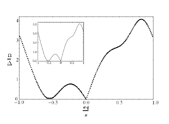
Figure 3: Collective-mode spectrum $\Omega(q)$ in 1D optical lattices for quasimomentum $p=0.21$ calculated by using the secular determinant (9). We set $f=0.5$ and $|U|=2J$. The superfluid gap and chemical potential are $\Delta=0.419J$ and $\mu=0.655J$. The insert shows the results from FIG. 4b in Ref. [Yosh, ], but calculated with $\Delta=0.420J$ and $\mu=0.624J$.

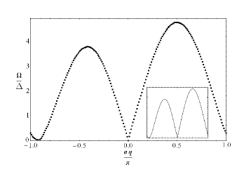
Figure 4: Collective-mode spectrum $\Omega(q)$ in 1D optical lattices for quasimomentum $p=0.12$ calculated by using determinant (9). We set $f=0.9$ and $|U|=2J$. The superfluid gap and chemical potential are $\Delta=0.351J$ and $\mu=1.697J$. The insert shows the results from FIG. 6b in Ref. [Yosh, ], but calculated with $\Delta=0.350J$ and $\mu=1.690J$.

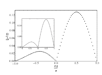
Figure 5: Collective-mode spectrum $\Omega(q)$ in 2D optical lattices for quasimomentum $\textbf{p}=(p,p)$, where $p=0.6502/\pi\sqrt{2}$ calculated by using the secular determinant (9). We set $f=0.5$ and $|U|=12J$. The superfluid gap and chemical potential are $\Delta=4.9699J$ and $\mu=0.7455J$. The insert shows the results from FIG. 9d in Ref. [Yosh, ] with the same $\Delta$ and $\mu$.

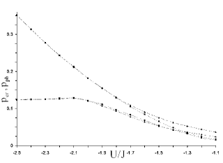
Figure 6: Critical $p_{cr}$ (lower curves) and pair-breaking $p_{pb}$ (upper curves) quasimomenta in units [$\pi/a$] as a functions of $U/J$ in 1D lattices and $f=0.9$. The dashed curves represent our calculations, while the dotted curves are the results presented in Fig. 7 in Ref. [Yosh, ]).

III Comparison with other approximations

Our numerical calculations show that there is an excellent agreement between the dispersions obtained by Ganesh et al. in Ref. [Gam, ] by using determinant (3), and by our secular determinant (9) not only in the case of a stationary lattice (see the conclusion section in Ref. [ZK1, ]), but in the case of a moving lattice as well. This is due to the fact that the terms with index $\widetilde{\gamma}$ in the secular determinant (9) are very small. This is due to the fact that the terms with index $\widetilde{\gamma}$ in the secular determinant (9) are very small.

In Fig. 3 and Fig. 4 we have compared the collective mode spectrum in 1D lattices obtained by the BS approach and by the Green’s function method.Yosh It is worth mentioning that in the 1D case our chemical potentials and gaps obtained from Eqs. (5) are not the same as in Ref. [Yosh, ], and therefore, the direct comparison between the corresponding dispersion curves is not correct, but the curves are quite similar. When using the same values for the chemical potential and the gap, our dispersion curve is slightly below the corresponding curve obtained in Ref. [Yosh, ] (see Fig. 5).

In Fig. 6 we have presented the critical $p_{cr}$ (lower curves) and pair-breaking $p_{pb}$ (upper curves) quasimomenta in 1D lattices as functions of $U/J$. The Green’s function and BS methods provide similar results for $-2.5<U/J<-1.8$, but in the interval $-1.7<U/J<-1.1$, both the pair-breaking and the critical quasimomentum curves differ from the corresponding curves presented in Fig. 7, Ref. [Yosh, ]. The differences between the pair-breaking curves are probably due to the different solutions of gap and number equations, but the differences between the critical momentum curves are most like due to the different techniques employed to obtain the collective-mode spectrum. It can be seen that according to our curves the Landau instability is still the mechanism which destabilized the superfluid states.

It is interesting to compare the analytical results for the speed of sound in a weak-coupling regime in 1D optical lattices obtained by both approaches. In a stationary lattice we follow the calculations by Belkhir and RanderiaBR to reduce our secular determinant (9) to the following $2\times 2$ determinant:

$$\left|\begin{array}[]{cc}-\frac{Q^{2}\alpha(\mu^{2}-4J\mu+\Delta^{2})}{4\Delta^{2}}-\frac{\omega^{2}\alpha}{4\Delta^{2}}&-\frac{\omega\alpha}{2\Delta}\\ -\frac{\omega\alpha}{2\Delta}&1-\alpha\end{array}\right|=0,$$ (11)

where $\alpha=|U|/(\pi\sqrt{4J\mu-\mu^{2}}$. The solution $\omega(Q)=cQ$ provides the speed of sound which in a stationary lattice is $c_{s}=\sqrt{1-\alpha}\sqrt{V_{F}^{2}-\Delta^{2}}$, where the Fermi velocity is $V_{F}=\sqrt{4J\mu-\mu^{2}}$. Using the same steps as in a stationary lattice, we have obtained the following $2\times 2$ determinant in 1D moving optical lattices:

$$\left|\begin{array}[]{cc}a_{11}&-\frac{\omega\alpha}{2\Delta}+\frac{(2J-\mu)Q\alpha\tan(p)}{2\Delta}\\ -\frac{\omega\alpha}{2\Delta}+\frac{(2J-\mu)Q\alpha\tan(p)}{2\Delta}&1-\alpha\end{array}\right|=0.$$ (12)

where $\alpha=|U|/(\pi\sqrt{4J^{2}\cos^{2}(p)-(2J-\mu)^{2}})$ and

$$a_{11}=-\frac{Q^{2}\alpha(\mu^{2}-4J\mu+\Delta^{2})}{4\Delta^{2}\cos^{2}(p)}-\frac{\omega^{2}\alpha}{4\Delta^{2}}+\frac{(2J-\mu)Q\alpha\omega\tan(p)}{2\Delta^{2}}-\frac{1}{4}Q^{2}\tan^{2}(p)-\frac{[2J^{2}-\Delta+4J^{2}\cos(2p)]Q^{2}\alpha\tan^{2}(p)}{2\Delta^{2}}.$$ (13)

The last determinant provides the following expression for the phononlike dispersion in the long-wavelength limit:

$$\begin{split}&c_{s}=(2J-\mu)\tan(p)+\sqrt{1-\alpha}\sqrt{V^{2}_{F}-\Delta^{2}\left[1+\frac{1-\alpha}{\alpha}\tan^{2}(p)\right]},\\ &V_{F}=\sqrt{4J^{2}\cos^{2}(p)-(2J-\mu)^{2}+4J^{2}\left[2-3\cos^{2}(p)\right]\tan^{2}(p)}.\end{split}$$ (14)

The speed of sound obtained in Ref. [Yosh, ] is

$$\begin{split}&c_{s}=(2J-\mu)\tan(p)+\sqrt{1-\alpha}\sqrt{V^{2}_{F}-\Delta^{2}\left[1+\frac{1-\alpha}{\alpha^{2}}\tan^{2}(p)\right]},\\ &V_{F}=\sqrt{4J^{2}\cos^{2}(p)-(2J-\mu)^{2}}.\end{split}$$ (15)

It should be mentioned that in the case when $\Delta/J<1$, the term $4J^{2}\left[2-3\cos^{2}(p)\right]\tan^{2}(p)$ is more important than the term $\Delta^{2}(1-\alpha)\tan^{2}(p)/\alpha$ in (14) and the term $\Delta^{2}(1-\alpha)\tan^{2}(p)/\alpha^{2}$ in (15).

IV Summary

In conclusion, we have derived the BS equation in GRPA for the collective-mode spectrum of superfluid Fermi gases in moving optical lattices assuming that the system is described by the attractive Hubbard model. We have compared collective excitation spectrum obtained by the BS approach with the corresponding spectrum obtained by applying the Green s function formalism and by the perturbation theory. The BS results are in an excellent agreement with the results obtained by perturbation theory, while the Green s function formalism provides slightly different results.

References

• (1) M. Greiner, C. A. Regal, and D. S. Jin, Nature (London) 426, 537 (2003).
• (2) S. Jochim, M. Bartenstein, A. Altmeyer, G. Hendl, S. Riedl, C. Chin, J. Hecker Denschlag, and R. Grimm, Science 302, 2101 (2003).
• (3) M. W. Zwierlein, C. A. Stan, C. H. Schunck, S. M. F. Raupach, S. Gupta, Z. Hadzibabic, and W. Ketterle, Phys. Rev. Lett. 91, 250401 (2003).
• (4) T. Bourdel, L. Khaykovich, J. Cubizolles, J. Zhang, F. Chevy, M. Teichmann, L. Tarruell, S. J. J. M. F. Kokkelmans, and C. Salomon, Phys. Rev. Lett. 93, 050401 (2004).
• (5) R. Ganesh, A. Paramekanti, and A. A. Burkov, Phys. Rev. A 80, 043612 (2009).
• (6) Y. Yunomae, D. Yamamoto, I. Danshita, N. Yokoshi, and S. Tsuchiya, Phys. Rev. A 80, 063627 (2009).
• (7) R. CotΓͺ and A. Griffin,, Phys. Rev. B 37, 4539 (1988).
• (8) H. Chu and Y. C. Chang, Phys. Rev. B 54, 5020 (1996).
• (9) R. CotΓͺ and A. Griffin, Phys. Rev. B, 48, 10404 (1993).
• (10) Z. Koinov, Phys. Rev. B 72, 085203 (2005).
• (11) R. Combescot, M. Yu. Kagan, and S. Stringari, Phys. Rev. A 74, 042717 (2006).
• (12) Z. G. Koinov, Physica Status Solidi (B), 247 ,140 (2010); Physica C 407, 470 (2010).
• (13) Z. G. Koinov, Ann. Phys. (Berlin) 522, 693 (2010).
• (14) P. W. Anderson, Phys. Rev. 112, 1900 (1958).
• (15) G. Rickayzen, Phys. Rev. 115, 795 (1959).
• (16) L. Belkhir and M. Randeria, Phys. Rev. B 49, 6829 (1994).
• (17) G. Baym and L. P. Kadanoff, Phys. Rev., 124, 287 (1961).