High-temperature surface superconductivity in topological flat-band systems

Abstract

We show that the topologically protected flat band emerging on a surface of a nodal fermionic system promotes the surface superconductivity due to an infinitely large density of states associated with the flat band. The critical temperature depends linearly on the pairing interaction and can be thus considerably higher than the exponentially small bulk critical temperature. We discuss an example of surface superconductivity in multilayered graphene with rhombohedral stacking.

Normal Fermi liquid is the generic form of a system of interacting fermions. Fermi liquid has a finite density of states (DOS) at zero energy, which may lead to instabilities at low $T$ with formation of broken symmetry states with smaller DOS. However, there is a class of fermionic systems with diverging DOS: the systems with a dispersionless spectrum that has exactly zero energy, i.e., the flat band. Historically this was first discussed in the context of Landau levels. However, flat bands may emerge also without a magnetic field, for example in strongly interacting condensed matter systems Khodel1990 ; NewClass ; Shaginyan2010 ; Gulacsi2010 , in layered systems with integer-valued pseudospin Dora2011 , in 2+1 dimensional quantum field theory dual to a gravitational theory in the anti-de Sitter background Sung-SikLee2009 , etc. In some cases the flat band is protected by topology in the momentum space: topologically protected zero modes emerge in cores of quantized vortices KopninSalomaa1991 ; Volovik2011 ; HeikkilaKopninVolovik10 , on surfaces of gapless topological media such as nodal superconductorsRyu2002 ; SchnyderRyu2010 ; HeikkilaKopninVolovik10 and multilayered grapheneGuineaCNPeres06 ; MakShanHeinz2010 ; HeikkilaVolovik10-1 ; HeikkilaKopninVolovik10 , as well as at the edges of graphene sheets Ryu2002 ; HeikkilaKopninVolovik10 .

In this report we consider a three dimensional (3D) system where the topologically protected flat band with its singular DOS appears on the surface giving rise to the 2D surface superconductivity. This property is generic and does not depend much on the details of the system. For illustration we use the multilayered graphene with rhombohedral stacking, where a surface flat band appears in the limit of large number of layers. We show that the superconducting critical temperature depends linearly on the pairing interaction strength and can be thus considerably higher than the usual exponentially small critical temperature in the bulk. This may open a new route to room-temperature superconductivity HeikkilaKopninVolovik10 . Formation of surface superconductivity is enhanced already for a system having $N\geq 3$ layers where the normal-state spectrum has a power-law dispersion $\xi_{p}\propto|{\bf p}|^{N}$ as a function of the in-plane momentum ${\bf p}$. The DOS $\nu(\xi_{p})\propto\xi_{p}^{(2-N)/N}$ has a singularity at zero energy which results in a drastic enhancement of the critical temperature. We also demonstrate that doping leads to a suppression of the surface critical temperature, contrary to its effect on the bulk superconductivity where the critical temperature is increased CastroNeto05 ; KopninSonin08 .

The model.

We consider multilayered graphene structure of $N$ layers in the discrete representation with respect to the interlayer coupling. We choose the rhombohedral stacking configuration considered in GuineaCNPeres06 ; MakShanHeinz2010 ; HeikkilaVolovik10-1 ; HeikkilaKopninVolovik10 and assume for simplicity that the most important are jumps between the atoms belonging to different sublattices parameterized by a single hopping energy $t$. More general form of the multilayered Hamiltonian can be found in Refs. McClure69 ; CastroNeto-review . In the superconducting case the Hamiltonian has the form of a matrix in the Nambu space. The Bogoliubov–de Gennes (BdG) equations are

$$\sum_{j=1}^{N}\left(\begin{array}[]{cc}\hat{H}_{ij}-\mu_{i}\delta_{ij}&\Delta_{i}\delta_{ij}\\ \Delta_{i}^{*}\delta_{ij}&-\hat{H}_{ij}+\mu_{i}\delta_{ij}\end{array}\right)\left(\begin{array}[]{c}\hat{u}_{j}\\ \hat{v}_{j}\end{array}\right)=E\left(\begin{array}[]{c}\hat{u}_{i}\\ \hat{v}_{i}\end{array}\right),$$

where the sum runs over the layers. The normal-state Hamiltonian HeikkilaVolovik10-1

$$\hat{H}_{ij}=v_{F}(\hat{\bm{\sigma}}\cdot{\bf p})\delta_{i,j}-t\hat{\sigma}_{+}\delta_{i,j+1}-t\hat{\sigma}_{-}\delta_{i,j-1}\ ,$$ (1)

$\hat{\bm{\sigma}}=(\hat{\sigma}_{x},\ \hat{\sigma}_{y})$, $\hat{\sigma}_{\pm}=(\hat{\sigma}_{x}\pm i\hat{\sigma}_{y})/2$, and $\hat{u}_{i},\ \hat{v}_{i}$ are matrices and spinors in the pseudo-spin space associated with two sublattices. This Hamiltonian acts on the envelope function of the in-plane momentum ${\bf p}$ taken near one of the Dirac points, i.e., for $|{\bf p}|\ll\hbar/a$ where $a$ is the interatomic distance within a layer; $v_{F}=3t_{0}a/2\hbar$ where $t_{0}$ is the the hopping energy between nearest-neighbor atoms belonging to different sublattices on a layer. The particle-like, $\hat{u}_{i}$, and hole-like, $\hat{v}_{i}$, wave functions near the Dirac point are coupled via the superconducting order parameter $\Delta_{i}$ that can appear in the presence of a pairing interaction. Here we do not specify the nature of pairing which can be either due to the electron-phonon interaction or due to other interactions that have been suggested as a source for intrinsic superconductivity in graphene, see Refs. pairing . As a reasonable starting point we assume $s$-wave symmetry of the order parameter and neglect fluctuations for simplicity, though they could, in principle, be relevant for 2D superconductivity. The excitation energy for particles and holes is measured upwards or downwards, respectively, from the Fermi level which can be shifted with respect to the Dirac point. We assume that the shifts at the outermost layers may be different from the bulk chemical potential due to the presence of a surface charge, i.e., $\mu_{i}=\mu$ for $i\neq 0,N$ while $\mu_{1,N}=\mu+\delta\mu_{1,N}$. The order parameter and the Fermi level shifts $\mu_{i}$ are scalars in the pseudo-spin space. We assume that $\Delta_{i}$ and $\mu_{i}$ are much smaller than the inter-layer coupling energy $t>0$, which in turn is $t\ll t_{0}$. Usually, $t\sim 0.1\,t_{0}$ where $t_{0}\sim 3$ eV CastroNeto-review .

Spectrum.

We decompose the wave function

$$\left(\begin{array}[]{c}\hat{u}_{n}\\ \hat{v}_{n}\end{array}\right)=\left[\left(\begin{array}[]{c}\alpha_{n}^{+}\\ \beta_{n}^{+}\end{array}\right)\otimes\hat{\Psi}^{+}+\left(\begin{array}[]{c}\alpha_{n}^{-}\\ \beta_{n}^{-}\end{array}\right)\otimes\hat{\Psi}^{-}\right]$$ (2)

into the spinor functions localized at each sublattice

$$\hat{\Psi}_{j}^{+}=\left(\begin{array}[]{c}1\\ 0\end{array}\right)\ ,\;\hat{\Psi}_{j}^{-}=\left(\begin{array}[]{c}0\\ 1\end{array}\right)\ .$$

The BdG equations take the form

$$\check{\tau}_{3}\left[v_{F}(p_{x}-ip_{y})\check{\alpha}_{n}^{-}-t\check{\alpha}_{n-1}^{-}-\mu\check{\alpha}_{n}^{+}\right]=E\check{\alpha}_{n}^{+},\;n\neq 1,\quad$$ (3)

$$\check{\tau}_{3}\left[v_{F}(p_{x}+ip_{y})\check{\alpha}_{n}^{+}-t\check{\alpha}_{n+1}^{+}-\mu\alpha_{n}^{-}\right]=E\check{\alpha}_{n}^{-},\;n\neq N.\quad$$ (4)

We introduce matrices and vectors in the Nambu space

$$\check{\tau}_{3}=\left(\begin{array}[]{lr}1&0\\ 0&-1\end{array}\right)\ ,\;\check{\Delta}_{n}=\left(\begin{array}[]{lr}0&\Delta_{n}\\ \Delta^{*}_{n}&0\end{array}\right)\ ,\;\check{\alpha}_{n}^{\pm}=\left(\begin{array}[]{c}\alpha_{n}^{\pm}\\ \beta_{n}^{\pm}\end{array}\right)\ .$$

In Eqs. (3) and (4) we assume that $\Delta_{n}\neq 0$ only at the outermost layers, while $\Delta_{n}=0$ for $n\neq 1,N$. The arguments supporting this model are given below. We also neglect $\Delta_{n}$ as compared to $t$ in Eqs. (3) and (4) for $n=N$ and $n=1$, respectively, as they lead to higher-order corrections in $\Delta/t$. The particle and hole channels are thus decoupled if $n\neq 1,N$ which determines the coefficients $\check{\alpha}_{n}^{\pm}=\check{A}^{\pm}e^{ip_{z}dn}$ and the energy in terms of the transverse momentum $p_{z}$ ($d$ is the interlayer distance) HeikkilaVolovik10-1

$$E^{2}=v_{F}^{2}p^{2}-2tv_{F}p\cos(p_{z}d-\phi)+t^{2}$$ (5)

where $p=\sqrt{p_{x}^{2}+p_{y}^{2}}$ and $e^{i\phi}=(p_{x}+ip_{y})/p$.

A finite order parameter $\Delta$ couples the particle and hole channels at the outermost layers, $i=1$ and $i=N$,

$$\check{\tau}_{3}v_{F}(p_{x}-ip_{y})\check{\alpha}_{1}^{-}-\check{\tau}_{3}\mu_{1}\check{\alpha}_{1}^{+} = E\check{\alpha}_{1}^{+}-\check{\Delta}_{1}\check{\alpha}_{1}^{+}\ ,$$ (6)

$$\check{\tau}_{3}v_{F}(p_{x}+ip_{y})\check{\alpha}_{N}^{+}-\check{\tau}_{3}\mu_{N}\check{\alpha}_{N}^{-} = E\check{\alpha}_{N}^{-}-\check{\Delta}_{N}\check{\alpha}_{N}^{-}\ .$$ (7)

Boundary conditions (6), (7) select $p_{z}$ and determine $2N$ particle and hole branches of the energy spectrum. Looking for the branches that belong to the surface states with energies of the order of $\Delta$ and $\mu$, we solve these equations for $E\ll t$. Since Eqs. (3), (4) do not contain $\Delta$, one can use the coefficients as obtained in Ref. HeikkilaVolovik10-1

$$\check{\alpha}^{+}_{n} = \frac{C}{\sqrt{2}}\left[\left(\frac{v_{F}p}{t}\right)^{n-1}\check{A}^{+}\right.$$

$$+\left.\left(\frac{v_{F}p}{t}\right)^{N-n}\frac{v_{F}p(\check{\tau}_{3}E+\mu)}{v_{F}^{2}p^{2}-t^{2}}\check{A}^{-}\right]e^{i(n-1-\frac{N}{2})\phi}\ ,$$

$$\check{\alpha}^{-}_{n} = \frac{C}{\sqrt{2}}\left[\left(\frac{v_{F}p}{t}\right)^{N-n}\check{A}^{-}\right.$$

$$+\left.\left(\frac{v_{F}p}{t}\right)^{n-1}\frac{v_{F}p(\check{\tau}_{3}E+\mu)}{v_{F}^{2}p^{2}-t^{2}}\check{A}^{+}\right]e^{i(n-\frac{N}{2})\phi}\ .$$

Here $C$ is a normalization constant. We include the first-order corrections in energy. Having an imaginary momentum $p_{z}$ for $v_{F}p<t$, these solutions decay away from the surfaces and thus they describe the surface states. The vectors $\check{A}^{\pm}=\left(A^{\pm},\,B^{\pm}\right)^{T}$ do not depend on $n$. Equations (6) and (7) yield

$$\check{\tau}_{3}\xi_{p}\check{A}^{-}=(\tilde{E}+\check{\tau}_{3}\tilde{\mu}_{1})\check{A}^{+}-\check{\Delta}_{1}\check{A}^{+}\ ,$$ (8)

$$\check{\tau}_{3}\xi_{p}\check{A}^{+}=(\tilde{E}+\check{\tau}_{3}\tilde{\mu}_{N})\check{A}^{-}-\check{\Delta}_{N}\check{A}^{-}\ ,$$ (9)

where $\xi_{p}=t\left(v_{F}p/t\right)^{N}$, $\tilde{\mu}_{1,N}=\tilde{\mu}+\delta\mu_{1,N}$, and

$$E=\tilde{E}(1-v_{F}^{2}p^{2}/t^{2}),\;\mu=\tilde{\mu}(1-v_{F}^{2}p^{2}/t^{2})\ .$$ (10)

Equations (8), (9) provide the surface-state spectrum

$$\left[\tilde{E}^{2}-\tilde{\mu}_{N}^{2}-|\Delta_{N}|^{2}\right]\left[\tilde{E}^{2}-\tilde{\mu}_{1}^{2}-|\Delta_{1}|^{2}\right]+\xi_{p}^{4}$$

$$-\xi_{p}^{2}\left[2\tilde{E}^{2}+2\tilde{\mu}_{1}\tilde{\mu}_{N}-\Delta_{1}^{*}\Delta_{N}-\Delta_{1}\Delta_{N}^{*}\right]=0\ .$$ (11)

Figure 1: (Color online): Spectrum of surface states for different numbers of layers. Left: $N=5$ and right: $N=50$. The symbols have been calculated by exact diagonalization and solid lines are computed from Eq. (12) up to the point where the approximation in it is valid. The three cases are: normal case with $\mu_{n}\equiv 0$ (blue circles), $\Delta=0.05t,\mu_{n}\equiv 0$ (red squares), and $\Delta=0.05t,\mu_{1}=\mu_{N}=0.03t$ (magenta crosses).

If $\Delta_{1}=\Delta_{N}$ we have from Eq. (11)

$$\tilde{E}^{2}_{\pm}=\left[\tilde{\mu}_{0}\mp\sqrt{\xi_{p}^{2}+(\delta\mu)^{2}}\right]^{2}+|\Delta|^{2}\ ,$$ (12)

where $\delta\mu=(\mu_{1}-\mu_{N})/2$ and $\tilde{\mu}_{0}=(\tilde{\mu}_{1}+\tilde{\mu}_{N})/2$. Equations (8), (9) determine four independent states. If $\mu=\delta\mu=0$ they are (i) $\tilde{E}_{1}=\tilde{E}$ and $A_{1}^{\pm}=u$, $B_{1}^{\pm}=v$, (ii) $\tilde{E}_{2}=-\tilde{E}$ and $A_{2}^{\pm}=v$, $B_{2}^{\pm}=-u$, (iii) $\tilde{E}_{3}=\tilde{E}_{0}$ and $A_{3}^{\pm}=\pm v$, $B_{3}^{\pm}=\pm u$, (iv) $\tilde{E}_{4}=-\tilde{E}$ and $A_{4}^{\pm}=\pm u$, $B_{1}^{\pm}=\mp v$. Here $\tilde{E}=\sqrt{\xi_{p}^{2}+\Delta^{2}}$ and

$$u=\frac{1}{\sqrt{2}}\left[1+\xi_{p}/\tilde{E}\right]^{\frac{1}{2}},\;v=\frac{1}{\sqrt{2}}\left[1-\xi_{p}/\tilde{E}\right]^{\frac{1}{2}}\ .\;$$ (13)

The overall normalization requires $d\sum_{n=1}^{N}[|\alpha^{+}_{n}|^{2}+|\beta^{+}_{n}|^{2}+|\alpha^{-}_{n}|^{2}+|\beta^{-}_{n}|^{2}]=1$. For $\xi_{p}\ll t$ this gives

$$|C|^{2}=d^{-1}[1-(v_{F}p/t)^{2}]\ .$$ (14)

Note that Eqs. (11)–(14) hold for $\xi_{p}\ll t$. The spectrum is plotted in Fig. 1.

If $N\to\infty$ and $\xi_{p}\to 0$ for any $v_{F}p/t<1$, the surface-state part localized at $n=N$ (with the coefficients $\check{A}^{-}$) decouples from that (with $\check{A}^{+}$) which is localized at $n=1$. For a “flat band” $\xi_{p}\to 0$, Eq. (11) yields

$$\tilde{E}^{2}_{+}=\tilde{\mu}_{N}^{2}+|\Delta_{N}|^{2}~{}{\rm or}~{}\tilde{E}^{2}_{-}=\tilde{\mu}_{1}^{2}+|\Delta_{1}|^{2}\ .$$ (15)

This shows that the definite signs in Eq. (12) belong to the surface states localized at the corresponding layers.

Flat band; zero doping.

The gap at a layer $N$ is

$$\Delta_{N} = \int\frac{d^{2}p}{(2\pi\hbar)^{2}}\sum_{k=1}^{N}V_{{\bf p},p_{z}(k)}{\rm Tr}\,[\hat{u}_{N}({\bf p},k)\hat{v}^{*}_{N}({\bf p},k)]$$

$$\times[1-2f(E_{{\bf p},k})],$$

where $f(E)$ is the Fermi distribution function. We assume that the cut-off momentum $p_{c}$ of the pairing potential $V$ is larger than $p_{\rm FB}=t/v_{F}$. The sum includes one $n=N$ surface state which we label by $k=0$ and the bulk states specified by the transverse momenta $p_{z}(k)$, where $k=1,2,\ldots,N-1$ with the spectrum of Eq. (5). Therefore, $\Delta_{N}=\Delta_{S}+\Delta_{B}$ where the surface contribution comes from the flat band area $p<p_{\rm FB}$,

$$\Delta_{S} = V\int_{p<p_{\rm FB}}\frac{d^{2}p}{(2\pi\hbar)^{2}}{\rm Tr}\,[\hat{u}_{N}({\bf p},0)\hat{v}^{*}_{N}({\bf p},0)]$$ (16)

$$\times[1-2f(E_{{\bf p},0})].\$$

The bulk contribution comes from the momenta $p>p_{\rm FB}$. For such momenta, the surface state $k=0$ will also extend to the bulk giving rise to (for $T=0$)

$$\Delta_{B}=V\int_{p_{\rm FB}<p<p_{c}}\frac{d^{2}p}{(2\pi\hbar)^{2}}\left\{{\rm Tr}\,[\hat{u}_{N}({\bf p},0)\hat{v}^{*}_{N}({\bf p},0)]\right.$$

$$+\left.\sum_{k=1}^{N-1}{\rm Tr}\,[\hat{u}_{N}({\bf p},k)\hat{v}^{*}_{N}({\bf p},k)]\right\}\ .$$ (17)

All the bulk states with $p>p_{\rm FB}$ are normalized to the sample width $W=dN$, i.e., $u^{*}(z)\sim 1/\sqrt{W}$. According to Eq. (5), $E\sim v_{F}p>t$ in Eq. (17). Therefore,

$$\Delta_{B}\approx\frac{Vp_{c}^{2}}{4\pi\hbar^{2}}\frac{N}{W}\left[\frac{\Delta}{v_{F}p_{c}}-{\cal O}\left(\frac{\Delta}{v_{F}p_{c}}\right)^{3}\right]\ .$$

If there was only the bulk contribution ($\Delta\equiv\Delta_{B}=\Delta_{N}$), the gap equation would have a nonzero solution only for a potential strength higher than a certain critical value $Vp_{c}/4\pi\hbar^{2}v_{F}d>1$, as is the case in the usual single-layer graphene with zero doping CastroNeto05 ; KopninSonin08 .

The surface states for $p<p_{\rm FB}$ are normalized according to Eq. (14). We find from Eq. (16)

$$\Delta_{S}=2V\int_{p<p_{\rm FB}}\frac{d^{2}p}{(2\pi\hbar)^{2}}|C|^{2}uv\tanh\frac{E}{2k_{B}T}\ .$$ (18)

For simplicity we assume that $V$ is constant up to the cut-off momentum $p_{c}$. Here $u$ and $v$ are determined by Eqs. (13), (14). In the case of a flat band $uv=1/2$ while $E=\Delta(1-v_{F}^{2}p^{2}/t^{2})$. For $T=0$ it gives

$$\Delta_{S}=\Delta_{0}\equiv g/8\pi\ ,$$ (19)

where $g=\tilde{V}p_{\rm FB}^{2}/\hbar^{2}$ is the characteristic pairing energy, $\tilde{V}=V/d$ is the two-dimensional pairing potential.

The ratio of the order parameter in the bulk to that on surface is of the order $(\Delta/t)(v_{F}p_{c}/t)$. Since $\Delta\ll t$, the contribution from the bulk states with $E>t$ can be neglected if the cut-off momentum of the interaction $p_{c}$ does not considerably exceed $t/v_{F}$. We thus arrive at the central result of our paper, namely that the surface superconductivity in the presence of a flat band dominates over the bulk superconductivity. This follows from an infinitely large density of states associated with the flat band. The critical temperature is determined by Eq. (19) with $\Delta\to 0$, which gives $\Delta_{0}=3k_{B}T_{c}$. Due to its linear dependence on the interaction strength, the critical temperature is proportional to the area of the flat band and can be essentially higher than that in the bulk.

For a flat band $\xi_{p}=0$ with $p_{c}=p_{\rm FB}$ the only characteristic values in the superconducting surface state are the energy $\Delta$ and the momentum $p_{\rm FB}$. Therefore, the coherence length should be of the order of the only available length scale, $\xi_{0}\sim\hbar/p_{\rm FB}$. It is much larger than the interatomic distance, $\xi_{0}\gg a$, since $p_{\rm FB}\ll p_{0}\sim\hbar/a$.

Doping destroys the surface superconductivity. This can be seen from Eq. (18) with $uv=\Delta/2\tilde{E}_{+}$ and $E=(1-v_{F}^{2}p^{2}/t^{2})\tilde{E}_{+}$ where $\tilde{E}_{+}$ is taken from Eq. (15). The critical temperature is found by putting $\Delta=0$. For example, if $\mu$ and $\mu_{N}$ have the same sign, both $\Delta_{0}$ and $T_{c}$ vanish at the critical doping level that satisfies

$$1=\frac{\tilde{V}}{4\pi\hbar^{2}|\mu_{N}-\mu|}\left|\frac{1}{2}-\frac{\mu}{\mu_{N}-\mu}+\frac{\mu^{2}}{(\mu_{N}-\mu)^{2}}\ln\frac{\mu_{N}}{\mu}\right|\ .$$

If $\mu_{N}=\mu$ the critical doping is $|\mu|=2k_{B}T_{c}$.

Surface superconductivity in a finite array.

Since the normal-state DOS defined as

$$\nu(\xi_{p})=\frac{p}{2\pi\hbar^{2}}\,\frac{dp}{d\xi_{p}}=\frac{t(\xi_{p}/t)^{\frac{2-N}{N}}}{2\pi\hbar^{2}Nv_{F}^{2}}\$$ (20)

has a low-energy singularity for $N>2$, the surface superconductivity is favorable already for a system with a finite number of layers $N\geq 3$. A simple expression for the zero-temperature gap can be obtained if $N\geq 5$. For a finite $N$, the value $\xi_{p}$ can reach values larger than $\Delta$. We use Eqs. (12) - (14) for zero doping in Eq. (18) where the upper limit of integration $p_{c}$ is now such that $\xi_{c}=t(v_{F}p_{c}/t)^{N}\gg\Delta$. Transforming to the energy integral with the normal-state DOS Eq. (20) we see that, for $N>4$, the integral converges at $\xi_{p}\sim\Delta$ or $p\sim p_{\Delta}=p_{\rm FB}(\Delta/t)^{\frac{1}{N}}$. The zero-temperature gap is

$$\Delta_{0}=t\left(\frac{g}{4\pi t}\left[\alpha(N)-\frac{1}{2}\left(\Delta_{0}/t\right)^{\frac{2}{N}}\alpha(N/2)\right]\right)^{\frac{N}{N-2}}$$ (21)

where

$$\alpha(N)=\int_{0}^{\infty}\frac{x^{\frac{N+2}{N}}\,dx}{\sqrt{x^{2}+1}^{3}}=\frac{1}{\sqrt{\pi}}\Gamma\left(\frac{N-2}{2N}\right)\Gamma\left(\frac{N+1}{N}\right)\ .$$

For $N\gg 1$ we have $\alpha_{N}=1$. The flat-band result, Eq. (19), is recovered if the number of layers is $N\gg 2\ln(t/\Delta_{0})$. The coherence length for a finite system is $\xi_{0}\sim\hbar/p_{\Delta}$. It approaches $\hbar/p_{\rm FB}$ for $N\to\infty$.

The gap obtained by numerical integration of Eq. (18) with a cut-off $p_{c}$ is plotted in Fig. 2, left panel. The right panel of Fig. 2 shows the order parameter as a function of the transverse coordinate. It extends into the bulk only over a few interlayer distances due to a decay of the wave functions. Taking this into account we have chosen the model, Eqs. (3)–(7), in which the order parameter is nonzero only on the outermost layers.

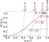
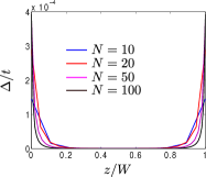
Figure 2: (Color online) Left panel: Zero-temperature gap as a function of the momentum cutoff $p_{c}$ for various $N$ (solid lines). The gap saturates at $p_{c}\sim p_{\Delta}$ and approaches Eq. (19) for $N\to\infty$. The dashed lines show the dispersion $\xi_{p}$ for each $N$. Right panel: the self-consistently calculated $\Delta(z)$ profile at different layers, $z=nd$. On both panels $g=0.01t$.

Conclusion.

The flat band with infinite DOS emerges in semi-metals with topologically protected nodal lines. The flat band promotes surface superconductivity with $T_{c}$ proportional to the pairing interaction strength and to the area of the flat band in the momentum space which is determined by the projection of the nodal line onto the surface. The critical temperature can thus be considerably higher than the exponentially small $T_{c}$ in the bulk. Formation of surface superconductivity is enhanced already for a system with a number of layers $N\geq 3$ where the normal DOS has a singularity at zero energy. Topologically protected flat bands may also appear on interfaces, twin boundaries and grain boundaries in bulk 3D topological materials leading to an enhanced bulk $T_{c}$. Indications towards surface superconductivity have been seen in experiments on graphiteKopelevich01 ; Esquinazi08 . The enhanced superconducting density has been reported on twin boundaries in Ba(Fe_1-xCo_x)₂As₂ Moler2010 . These observations might be explicable with our theory. Our predictions may be used for search or for artificial fabrication of layered and/or twinned systems with high- and even room-temperature superconductivity.

References

• (1) V.A. Khodel and V.R. Shaginyan, JETP Lett. 51, 553 (1990).
• (2) G.E. Volovik, JETP Lett. 53, 222 (1991).
• (3) V.R. Shaginyan, M.Ya. Amusia, A.Z. Msezane, K.G. Popov, Phys. Rep. 492, 31–109 (2010).
• (4) Z. Gulacsi, A. Kampf and D. Vollhardt, Phys. Rev. Lett. 105, 266403 (2010).
• (5) B. Dora, J. Kailasvuori and R. Moessner, arXiv:1104.0416.
• (6) Sung-Sik Lee, Phys. Rev. D 79, 086006 (2009).
• (7) N.B. Kopnin and M.M. Salomaa, Phys. Rev. B 44, 9667–9677 (1991).
• (8) G.E. Volovik, JETP Lett. 93, 66–69 (2011).
• (9) T.T. Heikkilä, N.B. Kopnin, and G.E. Volovik, arXiv:1012.0905.
• (10) S. Ryu and Y. Hatsugai, Phys. Rev. Lett. 89, 077002 (2002).
• (11) A.P. Schnyder and Shinsei Ryu, arXiv:1011.1438; P.M.R. Brydon, A.P. Schnyder, and C. Timm, arXiv:1104.2257.
• (12) F. Guinea, A.H. Castro Neto, and N.M.R. Peres, Phys. Rev. B 73, 245426 (2006).
• (13) T.T. Heikkilä and G.E. Volovik, JETP Lett. 93, 59–65 (2011).
• (14) Kin Fai Mak, Jie Shan, and T.F. Heinz, Phys. Rev. Lett. 104, 176404 (2010).
• (15) B. Uchoa, G.G. Cabrera, and A.H. Castro Neto, Phys. Rev. B, 71, 184509 (2005).
• (16) N.B. Kopnin and E.B. Sonin, Phys. Rev. Lett. 100, 246808 (2008).
• (17) J.W. McClure, Carbon 7, 425 (1969).
• (18) A.H. Castro Neto, F. Guinea, N.M.R. Peres, K.S. Novoselov, and A.K. Geim, Rev. Mod. Phys. 81, 109, 2009.
• (19) B. Uchoa and A. H. Castro Neto, Phys. Rev. Lett. 98, 146801 (2007); A. M. Black-Schaffer and S. Doniach, Phys. Rev. B, 75, 134512 (2007); C. Honerkamp, Phys. Rev. Lett. 100, 146404 (2008); see also review V.N. Kotov, B. Uchoa, V.M. Pereira, A.H. Castro Neto, and F. Guinea, arXiv: 1012.3484, and references therein.
• (20) R. Ricardo da Silva, J.H.S. Torres, and Y. Kopelevich, Phys. Rev. Lett. 87 147001, (2001).
• (21) P. Esquinazi, N. García, J. Barzola-Quiquia, P. Rödiger, K. Schindler, J.-L. Yao, and M. Ziese, Phys. Rev. B 78, 134516 (2008); S. Dusari, J. Barzola-Quiquia and P. Esquinazi, arXiv:1005.5676.
• (22) B. Kalisky, J.R. Kirtley, J.G. Analytis, Jiun-Haw Chu, A. Vailionis, I.R. Fisher, K.A. Moler, Phys. Rev. B 81, 184513 (2010).