Emergence of double scaling law in complex system

Abstract

We introduce a stochastic model to explain a double power-law distribution which exhibits two different Paretian behaviors in the upper and the lower tail and widely exists in social and economic systems. The model incorporates fitness consideration and noise fluctuation. We find that if the number of variables (e.g. the degree of nodes in complex networks or people’s incomes) grows exponentially, normal distributed fitness coupled with exponentially increasing variable is responsible for the emergence of the double power-law distribution. Fluctuations do not change the result qualitatively but contribute to the second-part scaling exponent. The evolution of Chinese airline network is taken as an example to show a nice agreement with our stochastic model.

1 Introduction

Power law behaviors are now pervasive in various kinds of studies [12, 3, 4, 11, 5, 6, 7, 1, 8, 2, 9, 10, 13, 14], which give an important class of complex networks, namely the scale-free networks. However, in some cases, such a single property is insufficient to describe the distributions in real-world systems in which scaling law is absent in some regions or, even more peculiar, changed at some critical points [15, 16]. In contrast to the typical power law, distribution including two different power-law regions is called double power-law whose cumulative distribution, namely the probability that variable $K$ is larger than a specific value $k$, is given by [16]:

$$P(K>k)=\{_{k^{-\gamma_{2}}\\ \\ ,~{}~{}k>k_{c}}^{k^{-\gamma_{1}}\\ \\ ,~{}~{}k<k_{c};}$$ (1)

where $\gamma_{1}$ and $\gamma_{2}$ are two scaling exponents while $k_{c}$ is the turning point. This kind of property exists widely in social and economic systems such as the degree distribution of airline network, word network or scientist collaboration network and the distribution of people’s incomes [16, 17, 18, 19, 20].

Some works related to double power law concentrate on how to fit such distribution by a uniform function rather than treat two power separately. Non-extensive statistical theory and the combination of different power-law functions were applied to the problem [22, 23]. However these works cannot tell us how this nontrivial property comes to its being. To understand its underlying mechanism, Reed proposed a model based on geometric Brownian motion [19]. He proved that such process coupled with exponential distributed evolution time causes, as he called, a double Pareto-lognormal distribution which has a lognormal body but power-law behaviour in both tails. This distribution is shown to provide an excellent fit to observed data on incomes and earnings. Dorogovtsev and Mendes proposed another different model aiming to explain the double power-law degree distribution in word network [24]. The model is constructed by two mechanisms: the preferential attachment and the creation of new links between old nodes which increases with evolution time. By continues approach, they show the degree distribution has two different scaling exponents, $-1.5$ for upper tail and $-3$ for lower tail.

Although the above two models can explain incomes and word network respectively, both of them have limitations. In word network model the scaling exponents are fixed. Thus it cannot explain the distributions with distinct scaling exponents. While in Reed’s model, the relative increase rate of incomes is assumed to be the same for all people. This is far from our knowledge that persons have heterogeneous ability of making money. Therefore fitness character must be taken into account to generalize the model. Besides, although the previous models reproduced some characters, the evolution of the real-world systems have not been investigated to support their model assumptions.

In this Letter, a general stochastic model is developed to explain the double power-law distribution. The model incorporates fitness consideration and noise fluctuation, which is general to describe many real-world system evolution. We find normal distributed fitness coupled with exponentially increasing variables is responsible for the emergence of the double power-law distribution while fluctuation does not change the result qualitatively but contribute to the scaling exponent. We also investigate the evolution of CAN to provide evidence for the proposed model.

2 Generalized model for double power law

Let’s denote $k_{i}(t,t^{\prime})$ the value at time $t$ of the $i$-th variable which comes into the system at time $t^{\prime}$ and denote $N(t)$ the number of the total variables in the system at time $t$. Regardless of the specific meaning of $k_{i}(t,t^{\prime})$, its evolution pattern usually shares common features. For an example, the increasing rate of $k_{i}$ is proportional to $k_{i}$ itself. This is probably caused by the preferential attachment (also called the rich get richer) that widely exists in self-organized complex systems [4]. Besides, it is natural to assume that the increasing rate is proportional to some of its own attributes which is called fitness, denoted as $\eta_{i}$ [25]. In reality fitness can be interpreted as, for examples, capital, social skills, activity levels of individuals and population or Gross Domestic Product (GDP) of cities. The increasing rate can also be influenced by other ingredients which can be normalized to be a time-dependent factors. But as the first step, let us focus on the simplest case where such factors are treated as constants. In this context, the evolution equation of $k_{i}(t,t^{\prime})$ is given by:

$$\frac{dk_{i}}{dt}=\eta_{i}k_{i}.$$ (2)

Thus $k_{i}$ grows exponentially as $k_{i}(t,t^{\prime})=e^{\eta_{i}(t-t^{\prime})}$ (assuming $k_{i}(t^{\prime},t^{\prime})=1$). This directly restricts the form of $N(t)$ in some systems such as node degree evolution in a network. Limited by its structure, the exponentially growing degree $k_{i}$ requires the exponentially growing $N(t)$ (or even faster). Although in some cases such as people’s incomes $N(t)$ does not encounter this problem, it has also been assumed to increase exponentially [19]. Therefore we assume

$$N(t)\propto e^{c_{n}t}.$$ (3)

The distribution of fitness $\eta_{i}$ is critical in our model. As we will analyze, normal distributed $\eta_{i}$ is essential to produce the double power-law distribution. Note that when we choose the specific parameters for $\eta_{i}$ in a network-structured system, we meet with the similar problem to $N(t)$. Since degree of a node can not exceed $n(t)-1$, to keep a long time evolution $\eta_{i}$ should be restricted so that the mean value of $\eta_{i}$, denoted as $\mu_{\eta}$, cannot be far larger than $c_{n}$ while the standard variance, denoted as $\sigma_{\eta}$, should be bounded properly.

Now let us turn to analyze the distribution under the above-mentioned condition. Using equation $p(k_{i}(t,t^{\prime}))dk_{i}(t,t^{\prime})=f(\eta_{i})d\eta_{i}$, the distribution of $k_{i}(t,t^{\prime})$ is easily derived to follow a lognormal distribution. Since the variables are added exponentially, their lifetime, defined as $T=t-t^{\prime}$, follows exponential distribution. Therefore the value of $k_{i}$ we actually examined is lognormal $k_{i}(T)$ mixed by exponentially distributed $T$. Thus the distribution reads:

$$p(k)=\int_{0}^{t_{c}}\frac{1}{\sqrt{2\pi}\sigma_{\eta}kT}e^{-\frac{(\ln(k)-\mu_{\eta}T)^{2}}{2\sigma_{\eta}^{2}T^{2}}}e^{-c_{n}T}dT,$$ (4)

where $t_{c}$ is the time when we examine $p(k)$. If $\sigma_{\eta}\rightarrow 0$, $\frac{1}{\sqrt{2\pi}\sigma_{\eta}kT}e^{-\frac{(\ln(k)-\mu_{\eta}T)^{2}}{2\sigma_{\eta}^{2}T^{2}}}\rightarrow\delta(T-\frac{\ln(k)}{\mu_{\eta}})$ and Eq.(4) gives:

$$p(k)\propto k^{-(1+\frac{c_{n}}{\mu_{\eta}})}\zeta(k-e^{\mu_{\eta}t_{c}}),$$ (5)

where $\zeta(k)=\{_{0\\ \\ ,~{}~{}k>0}^{1\\ \\ ,~{}~{}k\leq 0}$. The variables $k_{i}$ follow a power-law distribution with a cut-off at $k_{c}=e^{\mu_{\eta}t_{c}}$ which is the maximum value. On the other hand, $\frac{1}{\sqrt{2\pi}\sigma_{\eta}kT}e^{-\frac{(\ln(k)-\mu_{\eta}T)^{2}}{2\sigma_{\eta}^{2}T^{2}}}\rightarrow 0$ if $\sigma_{\eta}\rightarrow\infty$ and the integral becomes $k$ independent, indicating a uniform distribution. However this never happens in a network-structured system since $\sigma_{\eta}$ is limited as we have discussed.

For a finite $\sigma_{\eta}>0$, it is difficult to derive analytical result from Eq.(4). Therefore numerical experiments are applied to analyze the problem. The simulation is carried out by the following instructions. At each time step new variables increasing exponentially are added by initial value 1 and are assigned fitness chosen from a normal distribution. Then each variable increases its value according to Eq.(2). We simulate the cumulative distribution for different $\sigma_{\eta}$ as shown in Fig. 1. When $\sigma_{\eta}=0$, the distribution follows a power-law form with a cut-off at $e^{\mu_{\eta}t_{c}}$, as we have discussed above. With the increase of $\sigma_{\eta}$, the second part of the distributions decreases more and more slowly while their shapes seem to be a power law. It is noteworthy that the turning point occurs at about $k_{c}=e^{\mu_{\eta}t_{c}}$ which is exact the point at which the cut-off occurs for $\sigma_{\eta}=0$. Therefore the turning point is expected to increase with the evolution time $t_{c}$ as $k_{c}\sim e^{\mu_{\eta}t_{c}}$, as well demonstrated in Fig. 2.

Figure 1: Simulation of the cumulative distribution of variable $k_{i}$. The simulation is carried out with $\mu_{\eta}=0.15$, $N(t)=50e^{0.088t}$ and $t_{c}=30$. For other $\mu_{\eta}$ and exponential increasing $N(t)$, similar results can be obtained. The study is averaged over $50$ realizations.

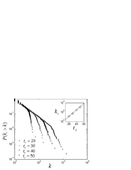
Figure 2: Simulation of the cumulative distribution of $k_{i}$ at different $t_{c}$. The simulation is carried out with $\mu_{\eta}=0.15$, $N(t)=50e^{0.088t}$ and $\sigma_{\eta}=0.02$. Inset: the correlation of $k_{c}$ and $t_{c}$. The fitted line (solid line) represents $y=0.6e^{0.15x}$, which illustrates that the turning point $k_{c}$ increases with $t_{c}$ as $k_{c}\sim e^{\mu_{\eta}t_{c}}$.

Another interesting discovery is that with the increase of $\sigma_{\eta}$, the first part of the distributions does not change significantly. From Fig. 1, we see that all the first part of the curves superpose the distribution of $\sigma_{\eta}=0$ well. Thus the first part of $p(k)$ must follow the same power-law distribution as the $p(k)$ of $\sigma_{\eta}=0$ with exponent $\gamma_{1}=\frac{c_{n}}{\mu_{\eta}}$ which is independent of $\sigma_{\eta}$. However $p(k)$ will finally become uniform distribution when $\sigma_{\eta}\rightarrow\infty$. There must have a transition point $\sigma_{tr}$ at which the first part of the distribution starts to change. By extensive numerical experiments, the transition point is determined to be $\sigma_{tr}\approx\frac{\mu_{\eta}}{2}$. The distributions of $\sigma_{\eta}>\sigma_{tr}$ are not studied since we only concern small $\sigma_{\eta}$. When $\sigma_{\eta}=\sigma_{tr}$, the second part of the distribution, as seen in Fig. 1, still decreases faster than $k^{-\frac{c_{n}}{\mu_{\eta}}}$. This result indicates that for all the $\sigma_{\eta}\leq\sigma_{tr}$, the second part of the distributions has an upper bound.

Now let us prove that the second part of $p(k)$ has a lower bound. It is easy to examine that when $\ln(k)>(\sigma_{\eta}\sqrt{\frac{\ln(t)}{t-1}}+\mu_{\eta})t$, the following inequality is valid:

$$\frac{1}{\sqrt{2\pi}\sigma_{\eta}kT}e^{-\frac{(\ln(k)-\mu_{\eta}T)^{2}}{2\sigma_{\eta}^{2}T^{2}}}e^{-c_{n}T}>$$

$$\frac{1}{\sqrt{2\pi T}\sigma_{\eta}k}e^{-\frac{(\ln(k)-\mu_{\eta}T)^{2}}{2\sigma_{\eta}^{2}T}}e^{-c_{n}T}.$$ (6)

Since $\sigma_{\eta}$ is usually very small, the above inequality is approximately considered to be valid when $\ln(k)>\mu_{\eta}T$. Therefore for any $k>e^{\mu_{\eta}t_{c}}$ (namely the second part of $p(k)$. The following discussion is restricted to this condition), the integral of the left term in Eq.(6) from 0 to $t_{c}$ must be larger than that of the right term. The integral of the left term is exactly the degree distribution $p(k)$ while the integral of the right term, according to Ref. [10], follows asymptotically a power-law function with the exponents related to $\mu_{\eta}$, $\sigma_{\eta}$ and $c_{n}$. Thus for a specific group of above exponents, $p(k)$ has a lower bound.

If $p(k)$ is not oscillatory, the existence of the upper and the lower bound allows $\frac{\ln(p(k))}{\ln(k)}$ to have a limitation. Assuming it to be $-\gamma$, then $p(k)$ is written as $p(k)\propto l(k)k^{-\gamma}$, where $l(k)\sim o(k^{\beta})$ and $k^{-\beta}\sim o(l(k))$ are valid for any $\beta>0$ when $k\rightarrow\infty$. Therefore for large $k$, given any constant $u>1$, we have the following inequality:

$$\frac{(uk)^{-\beta}}{k^{-\beta}}<\frac{l(uk)}{l(k)}<\frac{(uk)^{\beta}}{k^{\beta}}.$$ (7)

Let $\beta\rightarrow 0$, then we have

$$\lim_{k\rightarrow\infty}\frac{l(uk)}{l(k)}=1.$$ (8)

Note that Eq.(8) is also valid for any constant $0<u\leq 1$. This property of $l(k)$ follows directly from the requirement that $p(k)$ is asymptotically scale invariant. Thus, the form of $l(k)$ only controls the finite extent of the lower tail and will not affect its scaling exponent significantly. So the second part of the $p(k)$ is also power law. For further study, numerical simulation is applied to determine the exponent of the second part of $p(k)$, denoted as $\gamma_{2}$. It is found that

$$\gamma_{2}\sim\frac{1}{\sigma_{\eta}}.$$ (9)

The result is well demonstrated by the simulation as shown in Fig. 3. It is noteworthy that $\sigma_{\eta}\rightarrow 0$ leads to $\gamma_{2}\rightarrow\infty$. The second part of $p(k)$ degenerates naturally to be a cut-off. The exact formulation of $\gamma_{2}$ may also be related to $c_{n}$ and $\mu_{\eta}$, but extensive simulations indicate that $\gamma_{2}$ is much less sensitive to $c_{n}$(or $\mu_{\eta}$) than to parameter $\sigma_{\eta}$.

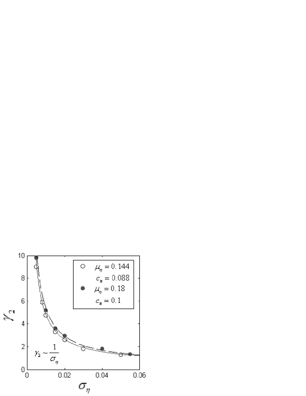
Figure 3: Numerical studies of $\gamma_{2}$. The evolution time $t_{c}$ is selected properly to keep the number of variables at about 1000 while the initial number of variables equals to 50. The fitted lines (solid line for $\mu_{\eta}=0.15$, $c_{n}=0.088$ and dashed line for $\mu_{\eta}=0.18$, $c_{n}=0.1$) is given by $\gamma_{2}=0.46+\frac{0.044}{\sigma_{\eta}}$ and $\gamma_{2}=0.44+\frac{0.05}{\sigma_{\eta}}$, respectively. The study is averaged over 50 realizations. For other $\mu_{\eta}$ and $c_{n}$, similar results can be obtained.

So far we have provided a possible model to produce double power-law distribution. However real complex systems such as the Internet or WWW usually include fluctuations that may be essential to describe the dynamics of its evolution [10, 21]. Therefore, a general model must be able to describe this feature. The generalization can be carried out by modifying Eq.(2):

$$\ d{k_{i}}=\rho\eta_{i}k_{i}dt+(1-\rho)(\mu_{\eta}dt+\sigma dw)k_{i},$$ (10)

where $dw$ is white noise of standard normal distribution and $\sigma$ is the standard variance of fluctuations. $\rho\in[0,1]$ is a parameter representing the relative contribution of the noise and the fitness, which can be considered as a measure of the degree of the disorder in real-world systems. Note that if $\rho=1$, Eq.(10) becomes Eq.(2) while if $\rho=0$, it leads to the geometric Brownian motion. Fluctuation described by the term $\sigma k_{i}dw$ is based on a general fact that in real systems such as WWW, site with large number of connections are likely to lose or gain more links than the site with small one. The solution of Eq.(10) is solved to be $e^{\rho\eta_{i}t}e^{(1-\rho)[(\mu_{\eta}-0.5\sigma^{2})t+\sigma w]}$ which follows lognormal distribution with logarithmic mean $\rho\mu_{\eta}t+(1-\rho)(\mu_{\eta}-0.5\sigma^{2})t$ and logarithmic variance $(\rho\sigma_{\eta}t)^{2}+(1-\rho)^{2}\sigma^{2}t$. By the similar methods used above, one can verify the distribution is still a double power law but the second scaling exponent is controlled by parameter $\rho$. In Fig. 4 we show the cumulative distribution for different $\rho$. It is found that the first part power-law behavior is still independent of $\rho$, leading to $\gamma_{1}=\frac{c_{n}}{\mu_{\eta}}$, but the second power-law exponent decreases with $\rho$. Therefore noise fluctuations do not change the distribution qualitatively but contribute to the second scaling exponent.

The present model (Eq.(10)) indicates that evolution of a complex system may be characterized by two parts: a leading ingredient influencing the evolution and noise fluctuations. This will be interpreted as follow. Since there are usually various ingredients related to the evolution of complex system, practically we cannot take all of them into account. A feasible method is to consider the most important ingredient as the fitness while all other minor ones as contributions to fluctuations. Then parameter $\rho$ represents how much the leading ingredient contributes to the evolution. If the evolution is totally governed by the leading ingredient, then $\rho\rightarrow 1$, indicating a deterministic pattern. On the other hand, if there is no apparent leading ingredient, it leads to $\rho\rightarrow 0$, indicating a random picture. Therefore our model is general to describe various real-world systems which evolve between order and disorder, and provide a better understanding on their evolution. As we will see in the following section, CAN is a typical example that follows such an evolution mechanism.

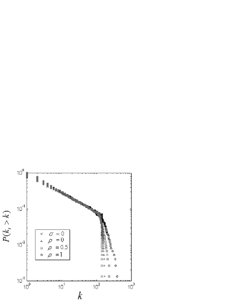
Figure 4: Numerical studies of the cumulative distribution for different $\rho$. The simulation is carried out with $\mu_{\eta}=0.17$, $N(t)=50e^{0.088t}$ and $t_{c}=30$. ’$\times$’ represents $\sigma_{\eta}=\sigma=0$ and the others represent $\sigma_{\eta}=\sigma=0.02$. When $\sigma_{\eta}=\sigma=0$ the distribution is a power law independent of $\rho$. When $\sigma_{\eta}=\sigma>0$, the first-part scaling exponent does not change while the second-part exponent decreases with $\rho$. The study is averaged over 50 realizations.

3 An example: Evolution of CAN

In this section, we will analyze the evolution of CAN to provide evidence for our proposed model.

Chinese airline system can be modeled as a complex network with cities representing nodes and flights representing edges. The degree of a node is defined as the sum of the airlines connecting to it. The degree distribution of CAN has been investigated by several studies which all indicate a double power-law behavior [16, 17, 22]. Here we will report some useful information. First we have analyzed the total number of nodes $N(t)$ existing at time $t$. It grows as $N(t)\propto e^{c_{n}t}$ with $c_{n}\approx 0.088$, which is consistent with our assumption that nodes increases exponentially. The number of edges $M(t)$ also increases exponentially with time as $M(t)\propto e^{c_{m}t}$ with $c_{m}\approx 0.154$. We have also measured the parameters of the degree distribution of CAN from 1999 to 2003 and a single year 2008, summarized in Table. 1. The exponent $\gamma_{1}$ stabilizes at about 0.51 while $\gamma_{2}$ fluctuates from 2.1 to 2.7. Note that the stabilization of $\gamma_{1}$ is indicated by our model where $\gamma_{1}$ is independent of fluctuations. The turning point $k_{c}$ shows an increase from 18 to 30, which is also consistent with our result that the turning point increases with evolution time.

In the present paper the evolution of CAN is studied by investigating the correlation between GDP and degree. The economic growth such as the size of tertiary industry has been recently demonstrated to be a leading ingredient in shaping the topology of CAN [26]. According to the discussion in the last section, we consider GDP relates to the fitness of the corresponding nodes. Note that the evolution of degree can also be studied by directly measuring the logarithmic ratio of the degree of successive two years. But this method can neither help to distinguish the identity of the fitness nor provide useful information of the corresponding parameters which is important in our analysis. As shown in Fig. 5, we found that the degree forms a linear function with its corresponding GDP ($R^{2}>0.62$) while the fluctuations are obvious. Despite the continuing evolution of both GDP and degree, this correlation has maintained for at least six years ($1998-2003$) since it has been first observed in $1998$. Therefore it provides some key information about the evolution of degree in CAN and cannot be viewed as just a coincidence.

Considering the time evolution, the correlation can be described as:

$$k_{i}(t)=D(t)G_{i}(t),$$ (11)

where $G_{i}(t)$ is the GDP of city $i$ at year $t$. It grows exponentially as $G_{i}(t)\propto e^{\lambda_{i}t}$ where $\lambda_{i}$ follows normal distribution with the mean of $0.18$ and the standard variance of 0.02. The strong positive correlation confirms that economy may govern the evolution of the degree in CAN while the fluctuations, as we mentioned previously, are considered to result from some minor ingredients (such as population density, public administration, geographical constraints, etc). Both the two aspects contribute to $D(t)$, leading to an expression given by $D(t)=e^{a(t)}e^{\varepsilon(t)}$, where term $e^{a(t)}$ is the time-dependent slope and the term $e^{\varepsilon(t)}$ represents the fluctuations.

Table 1: Two scaling exponents ($\gamma_{1}$ and $\gamma_{2}$) and the turning point ($k_{c}$) of cumulative degree distribution in CAN

	1999	2000	2001	2002	2003	2008
$\gamma_{1}$	0.46	0.51	0.52	0.51	0.51	0.51
$\gamma_{2}$	2.2	2.1	2.5	2.3	2.7	2.7
$k_{c}$	18	18	20	21	22	30

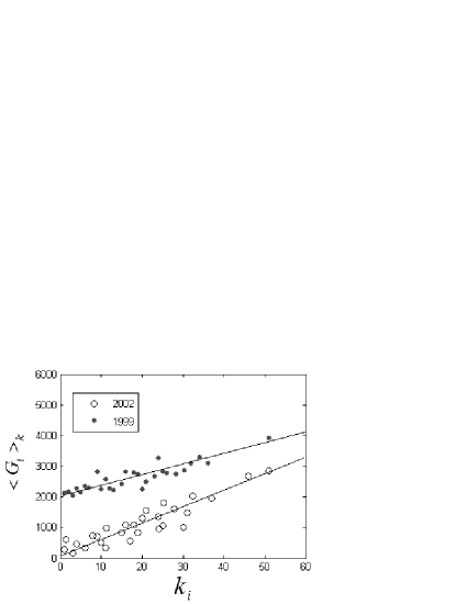
Figure 5: The correlation of degree and its corresponding GDP for year 1999 and year 2002. Both of them exhibit linear correlation. $\langle G_{i}(t)\rangle_{k}$ is an average over all the nodes with the same degree $k$. Note that the data of the two years are not drawn for better visualization. ($G_{i}(1999)$ here increases 2000 from the origin data.) The correlation does not change from 1998 to 2003.

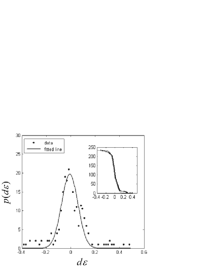
Figure 6: The distribution of the increment of $\varepsilon(t)$ for all the five years. The data is binned into classes. The fitted line is $p(d\varepsilon)=19.4e^{(-\frac{(d\varepsilon)^{2}}{2*0.09^{2}})}$. Therefore it follows normal distribution with mean 0 and standard variance 0.09. Inset: The cumulative distribution of $d\varepsilon(t)$. It is well fitted by $P(d\varepsilon(t)>d\varepsilon)=116erfc(\frac{d\varepsilon}{0.127})$ where $erfc(x)=\frac{2}{\sqrt{\pi}}\int_{x}^{\infty}e^{-x^{2}}dx$.

The specific form of $a(t)$ is easy to be evaluated. Summing Eq.(11) for all nodes we get $\langle D(t)\rangle=e^{a(t)}=\frac{2M(t)}{\sum_{i}G_{i}(t)}\sim e^{-0.036t}$, where $\sum_{i}G_{i}(t)$ is measured to be proportional to $e^{0.19t}$. Thus $a(t)=-0.036t$. Then $\varepsilon(t)$ can be investigated from data by calculating $\varepsilon(t)=\ln(\frac{k_{i}(t)}{G_{i}(t)})-a(t)$. However what we concern here is the increment of $\varepsilon(t)$, defined as $d\varepsilon(t)=\varepsilon(t)-\varepsilon(t-1)$. In Fig. 6 we plot the distribution of $d\varepsilon(t)$ for all the five years. It follows a normal distribution with the mean of 0 and the standard variance of 0.09. Furthermore we calculate the self-correlation function of $d\varepsilon(t)$, defined as $\langle d\varepsilon(t)d\varepsilon(t+\tau)\rangle=\frac{1}{N(t)}\sum_{i}d\varepsilon_{i}(t)d\varepsilon_{i}(t+\tau)$ ($\tau$ is the time interval). As listed in Table. 2, it exhibits very weak correlation (correlation coefficient $<0.1$) when $\tau\neq 0$. Therefore $d\varepsilon(t)$ can be regarded as white noise and expressed as $d\varepsilon(t)=0.09dw$. Then $D(t)$ is written as $D(t)\sim e^{0.09w-0.036t}$. Substituting it into Eq.(11) and applying differentiation we have [27]

$$dk_{i}=(\lambda_{i}-0.036)k_{i}dt+0.09k_{i}dw.$$ (12)

Eq.(12) is exact the form of our model which can give rise to double power-law distribution. To further demonstrate its agreement with the real evolution of CAN, we simulate the degree distribution according to Eq.(12). We obtained $\gamma_{1}=0.61$ (it can also be calculated from $\gamma_{1}=\frac{c_{n}}{\mu_{\eta}}=\frac{c_{n}}{\langle\lambda_{i}\rangle-0.036}=0.61$), comparable to the first exponent 0.51 while $\gamma_{2}=2.84$, good agreement with the second exponent 2.7.

Table 2: The self-correlation function $\langle d\varepsilon(t)d\varepsilon(t+\tau)\rangle$

	1999	2000	2001	2002	2003
$1999$	1	0.041	-0.019	-0.02	-0.01
$2000$	0.041	1	-0.06	-0.023	0.06
$2001$	-0.019	-0.06	1	-0.1	0.01
$2002$	-0.02	-0.023	-0.1	1	-0.035
$2003$	-0.01	0.06	0.01	-0.035	1

4 Conclusion

We have proposed a general model to explain the emergence of the double power-law distribution. The model incorporates fitness consideration and noise fluctuation which indicates that evolution of a complex system may be characterized by two parts: a leading ingredient and noise fluctuations. We find that normal distributed fitness coupled with exponentially increasing variables is responsible for the emergence of the double power-law distribution. Fluctuations do not change the result qualitatively but contribute to the value of scaling exponent. We have also studied empirically the CAN which turns out to follow the same evolution pattern as our proposed model.

We have only discussed the behavior of our model when $\sigma_{\eta}<\frac{\mu_{\eta}}{2}$. If $\sigma_{\eta}$ is not much larger than $\frac{\mu_{\eta}}{2}$, the distribution still decays like a double power-law but both the exponents are different from previous ones. With the continuing increasing of $\sigma_{\eta}$, the double power-law behavior turns out to be unconspicuous. It results from that the second scaling exponent is gradually close to the first one and finally becomes indistinguishable.

Finally, we would like to mention that we have done tests for six usual distributions, namely exponential distribution, uniform distribution, power-law distribution, Poisson distribution, Rayleigh distribution and Weibull distribution for the fitness instead of normal distribution, the results show that none of them is able to achieve double power-law distribution. Therefore we believe that normal distribution of fitness is a key ingredient responsible for the double power-law distribution.

5 Acknowledgements

This work was partially supported by National Nature Science Foundation of China under Grant numbers 11075057, 11035009 and 10979074, and the Shanghai Development Foundation for Science and Technology under contract No. 09JC1416800.

References

- [1] Cohen R., Erez K., ben-Avraham D. and Havlin S., Phys. Rev. Lett. 85 (2000) 4626.
- [2] Cohen R. and Havlin S., Complex Networks: Structure, Robustness and Function (Cambridge University Press, Cambridge) 2010.
- [3] Clauset A, Shalizi C R, Newman M E J, SIAM Review 51 (2009) 661; Newman M E J, Contemporary Physics 46 (2005) 323
- [4] Barabási A L, Albert RScience 286 509; Barabási A L, Albert R, Jeong H, Physica A 272 (1999) 173
- [5] Semboloni F, Eur. Phys. J. B 63 (2008) 295
- [6] Ebel H, Mielsch L I, Bornholdt S, Phys. Rev. E 66 (2002) 035103
- [7] Amaral L A N, Scala A, Barthélémy M and Stanley H E, Proc. Natl. Acad. Sci. U.S.A., 97 (2000) 11149.
- [8] Callaway D S, Newman M E J, Strogatz S H and Watts D J, Phys. Rev. Lett. 85 (2000) 5468.
- [9] Lo’opez E., Buldyrev S V, Havlin S, and Stanley H E, Phys. Rev. Lett. 94 (2005) 248701; Wu Z, Braunstein L A, Havlin S, and Stanley H E, Phys. Rev. Lett. 96 (2006) 148702
- [10] Goh K I, Kahng B, Kim D, Phys. Rev. Lett. 88 (2002) 108701
- [11] Ma Y G, Phys. Rev. Lett., 83 (1999) 3617; Ma Y G et al., Phys. Rev. C 71 (2005) 054606.
- [12] Han D D, Liu J G, Ma Y G, Cai X Z, Shen W Q Chin. Phy. Lett. 21 (2004) 1855; Han D D, Liu J G, Ma Y G Chin. Phy. Lett. 25 (2008) 765
- [13] Qian J H, Han D D, Physica A 388 (2009) 4248
- [14] Newman M E J, SIAM Rev. 45 (2003) 167
- [15] Mossa S, Barthélémy M, Stanley H E, and Amaral L A N, Phys. Rev. Lett. 88 (2002) 138701
- [16] Li W, Cai X, Phy. Rev. E 69 (2004) 04610; Chi L P, Wang R, Su H, Xu X P, Zhao J S, Li W, Cai X, Chin. Phy. Lett. 20 (2003) 1393
- [17] Liu H K, Zhou T, Acta. Phys. Sin. 56 (2007) 0106
- [18] Newman M E J, Phys. Rev. E 64 (2001) 016131
- [19] Reed W J, Physica A 319 (2002) 469
- [20] Han D D, Qian J H, Liu J , Physica A 388 (2009) 71
- [21] Huuberman B A, Adamic L A, Nature 401 (1999) 131
- [22] Li W, Wang Q A, Nivanen L, Le Méhauté A Physica A 368 (2006) 262
- [23] Scarfone A M, Physica A 382 (2007) 271
- [24] Dorogovtsev S N, Mendes J F FProc. Royal Soc. London B 268 (2001) 2603
- [25] Jeong H, Néda Z, Barabási A L, Europhys. Lett. 61 (2003) 567
- [26] Liu H K, Zhang X L, Cao L, Wang B H, Zhou T, Sci. China Ser G 39 (2009) 935
- [27] Actually as well as defined here is time-discrete, therefore Eq.(12) is better to be expressed as a difference equation. However we omit rigor, for simplicity.