STOCHASTIC EXPONENTIAL INTEGRATORS FOR FINITE ELEMENT DISCRETIZATION OF SPDEs FOR MULTIPLICATIVE & ADDITIVE NOISE

Abstract

We consider the numerical approximation of a general second order semi–linear parabolic stochastic partial differential equation (SPDEs) driven by space-time noise, for multiplicative and additive noise. We examine convergence of exponential integrators for multiplicative and additive noise. We consider noise that is in trace class and give a convergence proof in the root mean square $L^{2}$ norm. We discretize in space with the finite element method and in our implementation we examine both the finite element and the finite volume methods. We present results for a linear reaction diffusion equation in two dimensions as well as a nonlinear example of two-dimensional stochastic advection diffusion reaction equation motivated from realistic porous media flow. Parabolic stochastic partial differential equation, finite element, exponential integrators, strong numerical approximation, multiplicative noise, additive noise.

1 Introduction

We analyse the strong numerical approximation of an Ito stochastic partial differential equation defined in $\Omega\subset\mathbb{R}^{d}$. Boundary conditions on the domain $\Omega$ are typically Neumann, Dirichlet or some mixed conditions. We consider

$$dX=(AX+F(X))dt+B(X)dW,\qquad X(0)=X_{0},\qquad t\in[0,T],\qquad T>0$$ (1.1)

in a Hilbert space $H$. Here $A$ is the generator of an analytic semigroup $S(t):=e^{tA},t\geq 0$ not neccessary self adjoint. The functions $F$ and $B$ are nonlinear of $X$ and the noise term $W(x,t)$ is a $Q$-Wiener process defined on a filtered probability space $(\mathbb{D},\mathcal{F},\mathbf{P},\left\{F_{t}\right\}_{t\geq 0})$, that is white in time. The noise can be represented as a series in the eigenfunctions of the covariance operator $Q$ given by

$$W(x,t)=\underset{i\in\mathbb{N}^{d}}{\sum}\sqrt{q_{i}}e_{i}(x)\beta_{i}(t),$$ (1.2)

where $(q_{i},e_{i})$, $i\in\mathbb{N}^{d}$ are the eigenvalues and eigenfunctions of the covariance operator $Q$ and $\beta_{i}$ are independent and identically distributed standard Brownian motions. Precise assumptions on $A$, $F$,$B$ and $W$ are given in Section 2 and under these type of technical assumptions it is well known, see [1, 2, 3] that the unique mild solution of (1.1) is given by

$$X(t)=S(t)X_{0}+\int_{0}^{t}S(t-s)F(X(s))ds+\int_{0}^{t}S(t-s)B(X(s))dW(s).$$ (1.3)

Typical examples of the above type of equation are stochastic (advection) reaction diffusion equations arising, for example, in pattern formation in physics and mathematical biology. We illustrate our work with both a simple reaction diffusion equation where we can construct an exact solution

$$dX=\left(\nabla\cdot\mathbf{D}\nabla X-\lambda X\right)dt+dW$$ (1.4)

as well as the stochastic advection reaction diffusion equation

$$dX=\left(\nabla\cdot\mathbf{D}\nabla X-\nabla\cdot(\mathbf{q}X)-\frac{X}{|X|+1}\right)dt+XdW,$$ (1.5)

where $\mathbf{D}$ is the diffusion tensor, $\mathbf{q}$ is the Darcy velocity field [4] and $\lambda$ is a constant depending of the reaction function. The study of numerical solutions of SPDEs is an active research area and there is an extensive literature on numerical methods for SPDEs (1.1). For temporal discretizations the linear implicit Euler scheme is often used [25, 29], spatial discretizations are usually achieved with finite element [30, 31, 27], finite difference [25, 29] or spectral Galerkin method [22, 5, 6, 7, 8].

In the special case with additive noise, new schemes using linear functionals of the noise have recently been considered [5, 6, 7, 8, 9, 10]. The finite element method is used for the spatial discretization in [9, 10] and the spectral Galerkin in [5, 6, 7, 8]. Our schemes here are based on using the finite element method (or finite volume method) for space discretization so that we gain the flexibility of theses methods to deal with complex boundary conditions and we can apply well developed techniques such as upwinding to deal with advection. One of our schemes is the non–diagonal version of the stochastic scheme presented in [22, 32] and the other is the extension of the deterministic exponential time differencing of order one [39] to stochastic exponential scheme. Comparing to the schemes presented in [9, 10] on additive noise, the results here are more general since the linear operator $A$ does not need to be self adjoint and we do not need information about eigenvalues and eigenfunctions of the linear operator $A$. Furthermore we examine here convergence for Ito multiplicative noise for the exponential integrators, which has not so far been considered for SPDEs for these integrators. As in [10], schemes presented here are based on exponential matrix computation, which is a notorious problem in numerical analysis [11]. However, new developments for both Léja points and Krylov subspace techniques [12, 13, 14, 15, 16, 17] have led to efficient methods for computing matrix exponentials. The convergence proof given below is similar to one in [28] for a finite element discretization in space and backward Euler based method in time. The paper is organised as follows. In Section 2 we present the two numerical schemes based on the exponential integrators and our assumptions on (1.1). We also present and comment on our convergence results. Section 3 contains the proofs of our convergence theorems. We conclude in Section 4 by presenting some simulations and discuss implementation of these methods.

2 Mild solution, numerical schemes and main results

2.1 The abstract setting and mild solution

Let us start by presenting briefly the notation for the main function spaces and norms that we use in the paper. We denote by $\|\cdot\|$ the norm associated to the inner product $(\cdot,\cdot)$ of the Hilbert space $H$. For a Banach space $\mathcal{V}$ we denote by $\|.\|_{\mathcal{V}}$ the norm of $\mathcal{V}$, $L(\mathcal{V})$ the set of bounded linear mapping from $\mathcal{V}$ to $\mathcal{V}$ and by $L_{2}(\mathbb{D},\mathcal{V})$ the space defined by

$$L_{2}(\mathbb{D},\mathcal{V}):=\left\{v\;\text{random variable with value in}\;\mathcal{V}:\;\mathbf{E}\|v\|_{\mathcal{V}}^{2}=\int_{\mathbb{D}}\|v(\omega)\|_{\mathcal{V}}^{2}d\mathbf{P}(\omega)<\infty\right\}.$$ (2.1)

Let $Q:H\rightarrow H$ be a trace class operator. We introduce the spaces and notation we need to define the $Q$-Wiener process. An operator $T\in L(H)$ is Hilbert-Schmidt if

$$\|T\|_{HS}^{2}:=\underset{i\in\mathbb{N}^{d}}{\sum}\|Te_{i}\|^{2}<\infty,$$

where $(e_{i})$ is an orthonormal basis in H. The sum in $\|.\|_{HS}^{2}$ is independent of the choice of the orthonormal basis in $H$. We denote the space of Hilbert–Schmidt operators from $Q^{1/2}(H)$ to $H$ by $L_{2}^{0}:=HS(Q^{1/2}(H),H)$ and the corresponding norm $\|.\|_{L_{2}^{0}}$ by

$$\|T\,\|_{L_{2}^{0}}:=\|TQ^{1/2}\|_{HS}=\left(\underset{i\in\mathbb{N}^{d}}{\sum}\|TQ^{1/2}e_{i}\|^{2}\right)^{1/2},\qquad\ T\in L_{2}^{0}.$$

Let $\varphi$ be a $L_{2}^{0}-$ process, we have the following equality using the Ito’s isometry [1]

$$\mathbf{E}\|\int_{0}^{t}\varphi dW\|^{2}=\int_{0}^{t}\mathbf{E}\|\varphi\|_{L_{2}^{0}}^{2}ds=\int_{0}^{t}\mathbf{E}\|\varphi Q^{1/2}\|^{2}_{HS}ds,\qquad\qquad t\in[0,T].$$

Let us give some assumptions required both for the existence and uniqueness of the solution of equation (1.1) and for our convergence proofs below.

Assumption 2.1

The operator $A$ is the generator of an analytic semigroup $S(t)=e^{tA},\quad t\geq 0$.

In the Banach space $\mathcal{D}((-A)^{\alpha/2})$, $\alpha\in\mathbb{R}$, we use the notation $\|(-A)^{\alpha/2}.\|=:\|.\|_{\alpha}$. We recall some basic properties of the semigroup $S(t)$ generated by $A$.

Proposition 2.2

[Smoothing properties of the semigroup [18]]
Let $\alpha>0,\;\beta\geq 0$ and $0\leq\gamma\leq 1$, then there exist $C>0$ such that

$$\|(-A)^{\beta}S(t)\|_{L(H)} \leq Ct^{-\beta}\;\;\;\;\;\text{for }\;\;\;t>0$$

$$\|(-A)^{-\gamma}(\text{I}-S(t))\|_{L(H)} \leq Ct^{\gamma}\;\;\;\;\;\text{for }\;\;\;t\geq 0.$$

In addition,

$$(-A)^{\beta}S(t) = S(t)(-A)^{\beta}\quad\text{on}\quad\mathcal{D}((-A)^{\beta})$$

$$\text{If}\;\;\;\beta \geq \gamma\quad\text{then}\quad\mathcal{D}((-A)^{\beta})\subset\mathcal{D}((-A)^{\gamma}),$$

$$\|D_{t}^{l}S(t)v\|_{\beta} \leq Ct^{-l-(\beta-\alpha)/2}\,\|v\|_{\alpha},\;\;t>0,\;v\in\mathcal{D}((-A)^{\alpha/2})\;\;l=0,1,$$

where $D_{t}^{l}:=\dfrac{d^{l}}{dt^{l}}$.

We describe now in detail the assumptions that we make on the nonlinear terms $F$,$B$ and the noise $W$.

Assumption 2.3

[Assumption on the drift term $F$] There exists a positive constant $L>0$ such that $F$ is continuous in $H$ and satisfies the following Lipschitz condition

$$\|F(Z)-F(Y)\|\leq L\|Z-Y\|\qquad\forall\quad Z,\;Y\in H.$$

As a consequence, there exists a constant $C>0$ such that

$$\|F(Z)\| \leq \|F(0)\|+\|F(Z)-F(0)\|\leq\|F(0)\|+L\|Z\|\leq C(1+\|Z\|)\qquad\qquad Z\in H.$$

Assumption 2.4

[Assumption on the noise and the diffusion term $B$]
The covariance operator $Q$ is in reace class i.e. Tr($Q)<\infty$, and there exists a positive constant $L>0$ such that $B$ is continuous in $H$ and satisfies the following condition

$$\|B(Z)-B(Y)\|_{L_{2}^{0}}\leq L\|Z-Y\|\qquad\forall Z,Y\in H.$$

As a consequence, there exists a constant $C>0$ such that

$$\|B(Z)\|_{L_{2}^{0}} \leq \|B(0)\|_{L_{2}^{0}}+\|B(Z)-B(0)\|_{L_{2}^{0}}\leq\|B(0)\|_{L_{2}^{0}}+L\|Z\|\leq C(1+\|Z\|)\qquad\qquad Z\in H.$$

Theorem 2.5

[Existence and uniqueness [1]]
Assume that the initial solution $X_{0}$ is an $F_{0}-$measurable $H-$valued random variable and Assumption 2.3, Assumption 2.4 are satisfied. There exists a mild solution $X$ to (1.1) unique, up to equivalence among the processes, satisfying

$$P\left(\int_{0}^{T}\|X(s)\|^{2}ds<\infty\right).$$ (2.2)

For any $p\geq 2$ there exists a constant $C=C(p,T)>0$ such that

$$\underset{t\in[0,T]}{\sup}\mathbf{E}\|X(t)\|^{p}\leq C\left(1+\mathbf{E}\|X_{0}\|^{p}\right).$$ (2.3)

For any $p>2$ there exists a constant $C_{1}=C_{1}(p,T)>0$ such that

$$\mathbf{E}\underset{t\in[0,T]}{\sup}\|X(t)\|^{p}\leq C_{1}\left(1+\mathbf{E}\|X_{0}\|^{p}\right).$$ (2.4)

The following theorem proves a regularity result of the mild solution $X$ of (1.1).

Theorem 2.6

Assume that Assumption 2.3 and Assumption 2.4 hold. Let $X$ be the mild solution of (1.1) given in (1.3). If $X_{0}\in L_{2}(\mathbb{D},\mathcal{D}((-A)^{\beta/2})),\,\beta\in[0,1)$ then for all $t\in[0,T],\,X(t)\in L_{2}(\mathbb{D},\mathcal{D}((-A)^{\beta/2}))$ with

$$\left(\mathbf{E}\|X(t)\|_{\beta}^{2}\right)^{1/2}\leq C\left(1+\left(\mathbf{E}\|X_{0}\|_{\beta}^{2}\right)^{1/2}+\left(1+\mathbf{E}\|X_{0}\|^{2}\right)^{1/2}\right).$$

Proof Recall that if $X$ is the mild solution of (1.1), according to (2.1) we need to estimate $\left(\mathbf{E}\|X(t)\|_{\beta}^{2}\right)^{1/2}$ and check that

$$\left(\mathbf{E}\|X(t)\|_{\beta}^{2}\right)^{1/2}<\infty.$$

Recall that the mild solution is given by

$$X(t)=S(t)X_{0}+\int_{0}^{t}S(t-s)F(X(s))ds+\int_{0}^{t}S(t-s)B(X(s))dW(s)$$

then

$$\left(\mathbf{E}\|X(t)\|_{\beta}^{2}\right)^{1/2} \leq \left(\mathbf{E}\|S(t)X_{0}\|_{\beta}^{2}\right)^{1/2}+\left(\mathbf{E}\|\int_{0}^{t}S(t-s)F(X(s))ds\|_{\beta}^{2}\right)^{1/2}+\left(\mathbf{E}\|\int_{0}^{t}S(t-s)B(X(s))dW(s)\|_{\beta}^{2}\right)^{1/2}$$

$$= I+II+III.$$

Since $X_{0}\in L_{2}(\mathbb{D},\mathcal{D}((-A)^{\beta/2})),\,\beta\in[0,1)$, we obviouly have

$$I=\left(\mathbf{E}\|S(t)X_{0}\|_{\beta}^{2}\right)^{1/2}\leq C\,\left(\mathbf{E}\|X_{0}\|_{\beta}^{2}\right)^{1/2}.$$

As a consequence of Assumption 2.3 and the semigroup properties in Proposition 2.2 we have

$$II=\left(\mathbf{E}\|\int_{0}^{t}S(t-s)F(X(s))ds\|_{\beta}^{2}\right)^{1/2} \leq \int_{0}^{t}\left(\mathbf{E}\|S(t-s)F(X(s))\|_{\beta}^{2}\right)^{1/2}ds$$

$$\leq \int_{0}^{t}\left(\mathbf{E}\|(-A)^{\beta/2}S(t-s)F(X(s))\|^{2}\right)^{1/2}ds$$

$$\leq C\left(\int_{0}^{t}\|(-A)^{\beta/2}S(t-s)\|_{L(L^{2}(\Omega))}ds\right)\left(\underset{0\leq s\leq t}{\sup}\left(\mathbf{E}\left(1+\|X(s)\|\right)^{2}\right)^{1/2}\right)$$

$$\leq C\left(\int_{0}^{t}(t-s)^{-\frac{\beta}{2}}ds\right)\left(1+\underset{0\leq s\leq t}{\sup}\left(\mathbf{E}\|X(s)\|^{2}\right)^{1/2}\right)$$

$$\leq C\,\left(1+\underset{0\leq s\leq t}{\sup}\left(\mathbf{E}\|X(s)\|^{2}\right)^{1/2}\right).$$

Finally, Ito’s isometry and the consequence of Assumption 2.4 yields

$$III^{2} = \mathbf{E}\|\int_{0}^{t}S(t-s)B(X(s))dW(s)\|_{\beta}^{2}$$

$$= \int_{0}^{t}\mathbf{E}\|(-A)^{\beta/2}S(t-s)B(X(s))\|_{L_{2}^{0}}^{2}ds$$

$$\leq C\left(\int_{0}^{t}\|(-A)^{\beta/2}S(t-s)\|_{L(L^{2}(\Omega))}^{2}ds\right)\left(1+\underset{0\leq s\leq t}{\sup}\mathbf{E}\|X(s)\|^{2}\right)$$

$$\leq C\left(1+\underset{0\leq s\leq t}{\sup}\mathbf{E}\|X(s)\|^{2}\right),$$

thus

$$III\leq C\left(1+\left(\underset{0\leq s\leq t}{\sup}\mathbf{E}\|X(s)\|^{2}\right)^{1/2}\right).$$

Then, using (2.3) with $p=2$ yields

$$\left(\mathbf{E}\|X(t)\|_{\beta}^{2}\right)^{1/2} \leq C\,\left(1+\left(\mathbf{E}\|X_{0}\|_{\beta}^{2}\right)^{1/2}+\underset{0\leq s\leq t}{\sup}\left(\mathbf{E}\|X(s)\|^{2}\right)^{1/2}\right)$$

$$\leq C\,\left(1+\left(\mathbf{E}\|X_{0}\|_{\beta}^{2}\right)^{1/2}+\left(1+\mathbf{E}\|X_{0}\|^{2}\right)^{1/2}\right),$$

$$< \infty.$$

Then, if $X_{0}\in L_{2}(\mathbb{D},\mathcal{D}((-A)^{\beta/2})),\,\beta\in[0,1)$ then for all $t\in[0,T],\,X(t)\in L_{2}(\mathbb{D},\mathcal{D}((-A)^{\beta/2}))$.

More results about the regularity of the mild solution $X$ can be found in [40, 41].

2.2 Application to the second order semi–linear parabolic SPDEs

We assume that $\Omega$ has a smooth boundary or is a convex polygon of $\mathbb{R}^{d},\;d=1,2,3$. In the sequel of this paper, for convenience of presentation, we take $A$ to be a second order operator as this simplifies the convergence proof.

More precisely we take $H=L^{2}(\Omega)$ and consider the general second order semi–linear parabolic stochastic partial differential equation given by

$$dX(t,x)=\left(\nabla\cdot\textbf{D}\nabla X(t,x)-\mathbf{q}\cdot\nabla X(t,x)+f(x,X(t,x))\right)dt+b(x,X(t,x))dW(t,x),$$ (2.5)

$x\in\Omega,t\in[0,T]$ where $f,b:\Omega\times\mathbb{R}\rightarrow\mathbb{R}$ are two continuously differentiable functions with globally bounded derivatives.

In the abstract form given in (1.1), the linear operator is defined by

$$A = \underset{i,j=1}{\sum^{d}}\dfrac{\partial}{\partial x_{i}}\left(D_{i,j}\dfrac{\partial}{\partial x_{j}}\right)-\underset{i=1}{\sum^{d}}q_{i}\dfrac{\partial}{\partial x_{i}},$$ (2.6)

where we assume that $D_{i,j}\in L^{\infty}(\Omega),q_{i}\in L^{\infty}(\Omega)$ and that there exists a positive constant $c_{1}>0$ such that

$$\underset{i,j=1}{\sum^{d}}D_{i,j}(x)\xi_{i}\xi_{j}\geq c_{1}|\xi|^{2}\;\;\;\;\;\;\forall\xi\in\mathbb{R}^{d}\;\;\;x\in\overline{\Omega}\;\;\;c_{1}>0,$$ (2.7)

and $F:H\rightarrow H$, $B:H\rightarrow HS(Q^{1/2}(H),H)$ are defined by

$$(F(v))(x)=f(x,v(x)),\qquad(B(v)u)(x)=b(x,v(x))\cdot u(x),$$ (2.8)

for all $x\in\Omega,\;v\in H,\;u\in Q^{1/2}(H)$, with $H=L^{2}(\Omega)$. As the functions $f$ and $b$ are two continuously differentiable functions with globally bounded derivatives, the Nemytskii operator $F$ corresponding to $f$ and the multiplication operator $B$ defined in (2.8) satisfy Assumptions 2.3–2.4 for appropriate eigenfunctions such that $\underset{i\in\mathbb{N}^{d}}{\sup}\left[\underset{x\in\Omega}{\sup}|e_{i}(x)|\right]<\infty$ (see [40, Section 4 ]).

Notice that by the definitions of the operator $B$ and $\|.\|_{L_{2}^{0}}$, for $Y\in H=L^{2}(\Omega)$

$$\|B(Y)\|_{L_{2}^{0}}^{2}=\underset{i\in\mathbb{N}^{d}}{\sum}\|b(Y)Q^{1/2}e_{i}\|^{2},$$ (2.9)

where $b(Y)$ is the Nemytskii operator defined by

$$b(Y)(x)=b(x,Y(x))\qquad\qquad x\in\Omega.$$ (2.10)

We introduce two spaces $\mathbb{H}$ and $V$ where $\mathbb{H}\subset V$ that depend on the choice of the boundary conditions for the domain of the operator $A$ and the corresponding bilinear form. For Dirichlet boundary conditions we let

$$V=\mathbb{H}=H_{0}^{1}(\Omega)=\{v\in H^{1}(\Omega):v=0\;\;\text{on}\;\;\partial\Omega\},$$

and for Robin boundary conditions, Neumann boundary being a special case, we take $V=H^{1}(\Omega)$ and

$$\mathbb{H}=\left\{v\in H^{1}(\Omega):\partial v/\partial\nu_{A}+\alpha_{0}v=0\quad\text{on}\quad\partial\Omega\right\},\qquad\alpha_{0}\in\mathbb{R}.$$

See [19] for details. The corresponding bilinear form of $-A$ is given by

$$a(u,v)=\int_{\Omega}\left(\underset{i,j=1}{\sum^{d}}D_{i,j}\dfrac{\partial u}{\partial x_{j}}\dfrac{\partial v}{\partial x_{i}}+\underset{i=1}{\sum^{d}}q_{i}\dfrac{\partial u}{\partial x_{j}}v\right)dx\;\;\;\;\;\;\;u,v\in V$$ (2.11)

for Dirichlet and Neumann boundary conditions, and by

$$a(u,v)=\int_{\Omega}\left(\underset{i,j=1}{\sum^{d}}D_{i,j}\dfrac{\partial u}{\partial x_{j}}\dfrac{\partial v}{\partial x_{i}}+\underset{i=1}{\sum^{d}}q_{i}\dfrac{\partial u}{\partial x_{j}}v\right)dx+\int_{\partial\Omega}\alpha_{0}u\,v\,dx\;\;\;\;\;\;\;u,v\in V,$$ (2.12)

for Robin boundary conditions. According to Gårding’s inequality (see [23, 19]), there exists two positive constants $c_{0}$ and $\lambda_{0}$ such that

$$a(v,v)+c_{0}\|v\|^{2}\geq\lambda_{0}\|v\|_{H^{1}(\Omega)}^{2}\;\;\;\quad\quad\forall v\in V.$$ (2.13)

By adding and subtracting $c_{0}Xdt$ on the right hand side of (1.1), we have a new operator that we still call $A$ corresponding to the new bilinear form that we still call $a$ such that the following coercivity property holds

$$a(v,v)\geq\;\lambda_{0}\|v\|_{H^{1}(\Omega)}^{2}\;\;\;\;\;\forall v\in V.$$ (2.14)

Note that the expression of the nonlinear term $F$ has changed as we include the term $-c_{0}X$ in a new nonlinear term that we still denote by $F$. The coercivity property (2.14) implies that $A$ is a sectorial on $L^{2}(\Omega)$ i.e. there exists $C_{1},\,\theta\in(\frac{1}{2}\pi,\pi)$ such that

$$\|(\lambda I-A)^{-1}\|_{L(L^{2}(\Omega))}\leq\dfrac{C_{1}}{|\lambda|}\;\quad\quad\lambda\in S_{\theta},$$ (2.15)

where $S_{\theta}=\left\{\lambda\in\mathbb{C}:\lambda=\rho e^{i\phi},\;\rho>0,\;0\leq|\phi|\leq\theta\right\}$ (see [18, 19]). Then $A$ is the infinitesimal generator of bounded analytic semigroups $S(t):=e^{tA}$ on $L^{2}(\Omega)$ such that

$$S(t):=e^{tA}=\dfrac{1}{2\pi i}\int_{\mathcal{C}}e^{t\lambda}(\lambda I-A)^{-1}d\lambda,\;\;\;\;\;\;\;\;t>0,$$ (2.16)

where $\mathcal{C}$ denotes a path that surrounds the spectrum of $A$.

Functions in $\mathbb{H}$ satisfy the boundary conditions and with $\mathbb{H}$ in hand we can characterize the domain of the operator $(-A)^{r/2}$ and have the following norm equivalence [36, 37] for $r=1,2$

$$\|v\|_{H^{r}(\Omega)}\equiv\|(-A)^{r/2}v\|=:\|v\|_{r},\qquad\forall v\in\mathcal{D}((-A)^{r/2})=\mathbb{H}\cap H^{r}(\Omega).$$

2.3 Numerical schemes

We consider the discretization of the spatial domain by a finite element triangulation. Let $\mathcal{T}_{h}$ be a set of disjoint intervals of $\Omega$ (for $d=1$), a triangulation of $\Omega$ (for $d=2$) or a set of tetrahedra (for $d=3$) with maximal length $h$. Let $V_{h}\subset V$ denote the space of continuous functions that are piecewise linear over the triangulation $\mathcal{T}_{h}$. To discretize in space we introduce the projection $P_{h}$ from $L^{2}(\Omega)$ onto $V_{h}$ defined for $u\in L^{2}(\Omega)$ by

$$(P_{h}u,\chi)=(u,\chi)\qquad\forall\;\chi\in V_{h}.$$ (2.17)

The discrete operator $A_{h}:V_{h}\rightarrow V_{h}$ is defined by

$$(A_{h}\varphi,\chi)=(A\varphi,\chi)=-a(\varphi,\chi)\qquad\varphi,\chi\in V_{h}.$$ (2.18)

Like the operator $A$, the discrete operator $A_{h}$ is also the generator of an analytic semigroup $S_{h}:=e^{tA_{h}}$.

The semi–discrete in space version of the problem (1.1) is to find the process $X^{h}(t)=X^{h}(.,t)\in V_{h}$ such that for $t\in[0,T]$,

$$dX^{h}=(A_{h}X^{h}+P_{h}F(X^{h}))dt+P_{h}B(X^{h})dW,\qquad X^{h}(0)=P_{h}X_{0}.$$ (2.19)

The mild solution of (2.19) at time $t_{m}=m\Delta t,\;\;\Delta t>0\;$ is given by

$$X^{h}(t_{m}) = S_{h}(t_{m})P_{h}X_{0}+\int_{0}^{t_{m}}S_{h}(t_{m}-s)P_{h}F(X^{h}(s))ds$$ (2.20)

$$+\int_{0}^{t_{m}}S_{h}(t_{m}-s)P_{h}B(X^{h})dW(s).$$

Then, given the mild solution at the time $t_{m}$, we can construct the corresponding solution at $t_{m+1}$ as

$$X^{h}(t_{m+1}) = S_{h}(\Delta t)X^{h}(t_{m})+\int_{0}^{\Delta t}S_{h}(\Delta t-s)P_{h}F(X^{h}(s+t_{m}))ds$$

$$+\int_{t_{m}}^{t_{m+1}}S_{h}(t_{m+1}-s)P_{h}B(X^{h})dW(s).$$

To build the first numerical scheme, we use the following approximations

$$S_{h}(\Delta t-s)F(X^{h}(t_{m}+s)) \approx S_{h}(\Delta t)F(X^{h}(t_{m}))\;\;\;\;\;\;\;\;\;\;s\in[0,\;\Delta t],$$

$$S_{h}(t_{m+1}-s)P_{h}B(X^{h}(s)) \approx S_{h}(\Delta t)P_{h}B(X^{h}(t_{m}))\;\;\;s\in[t_{m},t_{m+1}].$$

We can define our approximation $Y_{m}^{h}$ of $X(m\Delta t)$ by

$$Y_{m+1}^{h} = e^{\Delta tA_{h}}\left(Y_{m}^{h}+P_{h}F(Y_{m}^{h})+P_{h}B(Y_{m}^{h})\Delta W_{m}\right)$$ (2.21)

$$= \varphi_{0}(\Delta tA_{h})\left(Y_{m}^{h}+P_{h}F(Y_{m}^{h})+P_{h}B(Y_{m}^{h})\Delta W_{m}\right),$$

where

$$\varphi_{0}(\Delta tA_{h}) := e^{\Delta tA_{h}},$$

$$\Delta W_{m} := W_{m+1}-W_{m}=\sqrt{\Delta t}\underset{i\in\mathbb{N}^{d}}{\sum}\sqrt{q_{i}}R_{i,m}e_{i},$$

with $R_{i,m}$ are independent, standard normally distributed random variables with means $0$ and variance $1$. We call the scheme in (2.21) SETDM0. To build the second numerical scheme, we use the following approximations

$$F(X^{h}(t_{m}+s)) \approx F(X^{h}(t_{m}))\;\;\;\;\;\;\;\;\;\;s\in[0,\;\Delta t],$$

$$S_{h}(t_{m+1}-s)P_{h}B(X^{h}(s)) \approx S_{h}(\Delta t)P_{h}B(X^{h}(t_{m}))\;\;\;s\in[t_{m},t_{m+1}].$$

We can define our approximation $X_{m}^{h}$ of $X(m\Delta t)$ by

$$X_{m+1}^{h}=e^{\Delta tA_{h}}X_{m}^{h}+A_{h}^{-1}\left(e^{\Delta tA_{h}}-I\right)P_{h}F(X_{m}^{h})+e^{\Delta tA_{h}}P_{h}B(X_{m}^{h})\left(W_{m+1}-W_{m}\right).$$ (2.22)

For efficiency we can rewrite the scheme (2.22) as

$$X_{m+1}^{h}=X_{m}^{h}+\Delta t\varphi_{1}(\Delta tA_{h})\left(A_{h}\left(X_{m}^{h}+P_{h}B(X_{m}^{h})\Delta W_{m}\right)+P_{h}F(X_{m}^{h})\right),$$

where

$$\varphi_{1}(\Delta tA_{h})=(\Delta t\,A_{h})^{-1}\left(e^{\Delta tA_{h}}-I\right)=\frac{1}{\Delta t}\int_{0}^{\Delta t}e^{(\Delta t-s)A_{h}}ds.$$

We call the scheme in (2.22) SETDM1. This scheme is also used in [24] with the Fourier method to solve fourth order stochastic problems.

2.4 Main result

Throughout the paper we take $t_{m}=m\Delta t\in(0,T]$, where $T=M\Delta t$ for $m,M\in\mathbb{N}$. We take $C$ to be a constant that may depend on $T$ and other parameters but not on $\Delta t$ or $h$. Our result is a strong convergence result in $L^{2}$ for schemes SETDM1 and SETDM0.

Theorem 2.7

Let $X(t_{m})$ be the mild solution of equation (1.1) at time  $t_{m}=m\Delta t,\;\Delta t>0$ represented by (1.3). Let $\zeta_{m}^{h}$ be the numerical approximations through (2.22) or (2.21) ($\zeta_{m}^{h}=X_{m}^{h}$ for scheme SETDM1 and $\zeta_{m}^{h}=Y_{m}^{h}$ for scheme SETDM0) and $0<\gamma<1$. Assume that $b(L_{2}(\mathbb{D},\mathcal{D}((-A)^{\alpha})))\subset L_{2}(\mathbb{D},\mathcal{D}((-A)^{\alpha}))$ for $\alpha\in(0,\gamma/10)$ small enough. The following estimates hold.

If $X_{0}\in L_{2}(\mathbb{D},\mathcal{D}((-A)^{\gamma})),\;0<\gamma\leq 1/2$ then

$$\left(\mathbf{E}\|X(t_{m})-\zeta_{m}^{h}\|^{2}\right)^{1/2} \leq C\left(t_{m}^{(-1+2\gamma)/2}h+\Delta t^{\gamma/2}\right).$$

If $X_{0}\in L_{2}(\mathbb{D},\mathcal{D}((-A)^{\gamma})),\;1/2\leq\gamma<1$ then

$$\left(\mathbf{E}\|X(t_{m})-\zeta_{m}^{h}\|^{2}\right)^{1/2} \leq C\left(h+\Delta t^{\gamma/2}\right).$$

Suppose that $F(L_{2}(\mathbb{D},\mathcal{D}((-A)^{\alpha^{\prime}})))\subset L_{2}(\mathbb{D},\mathcal{D}((-A)^{\alpha^{\prime}})),\;\alpha^{\prime}\in(0,\gamma/10)$ small enough:

If $X_{0}\in L_{2}(\mathbb{D},\mathcal{D}((-A)^{\gamma}))$ then

$$\left(\mathbf{E}\|X(t_{m})-\zeta_{m}^{h}\|^{2}\right)^{1/2} \leq C\left(t_{m}^{(-1+\gamma)}h^{2}+\Delta t^{\gamma/2}\right).$$

If $X_{0}\in L_{2}(\mathbb{D},\mathcal{D}(-A))$ and $b(L_{2}(\mathbb{D},\mathcal{D}(-A)))\subset L_{2}(\mathbb{D},\mathcal{D}(-A))$ then

$$\left(\mathbf{E}\|X(t_{m})-\zeta_{m}^{h}\|^{2}\right)^{1/2} \leq C\left(h^{2}+\Delta t^{(1/2-\epsilon)}\right).$$

$\epsilon\in(0,1/2)$, small enough.

Remark 2.8

In the proof of Theorem 2.7, the assumptions $b(L_{2}(\mathbb{D},\mathcal{D}((-A)^{\alpha})))\subset L_{2}(\mathbb{D},\mathcal{D}((-A)^{\alpha}))$ for $\alpha\in(0,\gamma/10)$ and $F(L_{2}(\mathbb{D},\mathcal{D}((-A)^{\alpha^{\prime}})))\subset L_{2}(\mathbb{D},\mathcal{D}((-A)^{\alpha^{\prime}})),\;\alpha^{\prime}\in(0,\gamma/10)$ are enough. We only need that $b(X(t))\in L_{2}(\mathbb{D},\mathcal{D}((-A)^{\alpha})),\;\alpha\in(0,\gamma/10)$ and $F(X(t))\in L_{2}(\mathbb{D},\mathcal{D}((-A)^{\alpha^{\prime}})),\;\ \alpha^{\prime}\in(0,\gamma/10),\;\;\forall\;t\in[0,T]$, where $X$ is the mild solution of equation (1.1).

Although we have taken the linear operator $A$ to be a second order operator, similar results will hold, for higher order operators. Computationaly, the noise given by (1.2) is truncated to $N$ terms. Therefore the corresponding approximated solutions become $X_{m}^{h,N}$ for SETDM1 and $Y_{m}^{h,N}$ for scheme SETDM0. For noise where the eigenvalues of the covariance operator have a strong exponential decay, $X_{m}^{h,N}$ and $Y_{m}^{h,N}$ are close to $X_{m}^{h}$ and $Y_{m}^{h}$ respectively. In the case of additive noise, it has been proved in [31] that with the truncation to $N$ terms of the noise (1.2) the corresponding discrete mild solution $X^{h,N}$ in (2.20) has the same order of accuracy respect to $h$ as $X^{h}$.

We also note that smooth noise improves the accuracy in Theorem 2.7 for additive noise (see [32] and Figure 1 in Section 4).

3 Proofs of the main results

3.1 Some preparatory results

We introduce the Riesz representation operator $R_{h}:V\rightarrow V_{h}$ defined by

$$(-AR_{h}v,\chi)=(-Av,\chi)=a(v,\chi)\qquad\qquad v\in V,\;\forall\chi\in V_{h}.$$

Under the regularity assumptions on the triangulation and in view of $V-$ellipticity (2.7), it is well known (see [19, 38]) that the following error bounds holds

$$\|R_{h}v-v\|+h\|R_{h}v-v\|_{H^{1}(\Omega}\leq Ch^{r}\|v\|_{H^{r}(\Omega)},\qquad v\in V\cap H^{r}(\Omega),\;\;r\in\{1,2\}.$$ (3.1)

We start by examining the deterministic linear problem. Find $u\in V$ such that such that

$$u^{\prime}=Au\qquad\text{given}\quad u(0)=v,\qquad t\in(0,T].$$ (3.2)

The corresponding semi-discretization in space is : Find $u_{h}\in V_{h}$ such that

$$u_{h}^{\prime}=A_{h}u_{h}$$

where $u_{h}^{0}=P_{h}v$. Define the operator

$$T_{h}(t):=S(t)-S_{h}(t)P_{h}=e^{tA}-e^{tA_{h}}P_{h}$$ (3.3)

so that $u(t)-u_{h}(t)=T_{h}(t)v$.

Lemma 3.1

The following estimate holds on the semi-discrete approximation of(3.2). If $v\in\mathcal{D}((-A)^{\beta/2})$

$$\|u(t)-u_{h}(t)\| = \|T_{h}(t)v\|\leq Ch^{r}t^{-(r-\beta)/2}\|v\|_{\beta}\;\;\;\;\;r\in\left\{1,2\right\}\;\;\beta\leq r,$$ (3.4)

where $r$ is related to (3.1).

Proof

The proof for $r=2$ and $\beta=0$ can be found in [[19], Theorem 7.1, page 817].
Set

$$u_{h}(t)-u(t)=\left(u_{h}(t)-R_{h}u(t)\right)+\left(R_{h}u(t)-u(t)\right)\equiv\theta(t)+\rho(t).$$ (3.5)

It is well known [36] that $A_{h}R_{h}=P_{h}A$. Indeed for $v\in\mathcal{D}(A),\;\chi\in V_{h}$ we have

$$(P_{h}Av,\chi) = (Av,\chi)\qquad\qquad\qquad\qquad\;\;\;(\text{by definition of $P_{h}$})$$

$$= (AR_{h}v,\chi)\qquad\qquad\qquad\qquad(\text{by definition of $R_{h}$})$$

$$= (A_{h}R_{h}v,\chi)\qquad\qquad\qquad\qquad(\text{since $R_{h}v\in V_{h}$})$$

thus $A_{h}R_{h}=P_{h}A$. We therefore have the following equation in $\theta$

$$\theta_{t}=A_{h}\theta-P_{h}D_{t}\rho.$$

Hence

$$\theta(t)=S_{h}(t)\theta(0)-\int_{0}^{t}S_{h}(t-s)P_{h}D_{s}\rho ds.$$

Splitting the integral up into two intervals and integration by parts over the first interval yields

$$\theta(t)=S_{h}(t)\theta(0)+S_{h}(t)P_{h}\rho(0)-S_{h}(t/2)P_{h}\rho(t/2)+\int_{0}^{t/2}\left(D_{s}S_{h}(t-s)\right)P_{h}\rho(s)ds-\int_{t/2}^{t}S_{h}(t-s)P_{h}D_{s}\rho(s)ds,$$

with $D_{s}=\partial/\partial s$. Since $\theta(t)\in V_{h}$ we therefore have $P_{h}\theta(t)=\theta(t)$, then

$$\theta(t)=S_{h}(t)P_{h}T_{h}(0)v-S_{h}(t/2)P_{h}\rho(t/2)+\int_{0}^{t/2}\left(D_{s}S_{h}(t-s)\right)P_{h}\rho(s)ds-\int_{t/2}^{t}S_{h}(t-s)P_{h}D_{s}\rho(s)ds.$$

Since

$$P_{h}T_{h}(0)v=P_{h}(v-P_{h}v)=0,$$

we therefore have

$$\theta(t)=-S_{h}(t/2)P_{h}\rho(t/2)+\int_{0}^{t/2}D_{s}S_{h}(t-s)P_{h}\rho(s)ds-\int_{t/2}^{t}S_{h}(t-s)P_{h}D_{s}\rho(s)ds.$$

Using the fact that $S_{h}$ and $P_{h}$ are uniformly bounded independently of $h$ with the smoothing property of $S_{h}$ in Proposition 2.2 yields

$$\|\theta(t)\|\leq C\left(\|\rho(t/2)\|+\int_{0}^{t/2}(t-s)^{-1}\|\rho(s)\|ds+\int_{t/2}^{t}\|D_{s}\rho(s)\|ds\right).$$

The estimate (3.1) with the smoothing property of $S(t)$ in Proposition 2.2 yields

$$\left\{\begin{array}[]{l}\|\rho(t)\|\leq Ch^{r}\|u\|_{r}\leq Ch^{r}t^{-(r-\beta)/2}\|v\|_{\beta}\\ \newline \\ \|D_{s}\rho(t)\|\leq Ch^{r}\|D_{s}u\|_{r}\leq Ch^{r}t^{-1-(r-\beta)/2}\|v\|_{\beta},\;\;\;\ r\in\left\{1,2\right\},\;\;\beta\leq r,\;\;\;v\in\mathcal{D}((-A)^{\beta/2}).\end{array}\right.$$

Then

$$\|\theta(t)\|\leq Ch^{r}t^{-(r-\beta)/2}\|v\|_{\beta}+Ch^{r}\|v\|_{\beta}\left(\int_{0}^{t/2}(t-s)^{-1}s^{-(r-\beta)/2}ds+\int_{t/2}^{t}s^{-1-(r-\beta)/2}ds\right).$$

Since

$$\int_{0}^{t/2}(t-s)^{-1}s^{-(r-\beta)/2}ds+\int_{t/2}^{t}s^{-1-(r-\beta)/2}ds\leq Ct^{-(r-\beta)/2},$$

we therefore have

$$\|T_{h}(t)v\|\leq\|\theta(t)\|+\|\rho(t)\|\leq Ch^{r}\;t^{-(r-\beta)/2}\|v\|_{\beta}.$$

Our second preliminary lemma concerns the mild solution SPDE of (1.1).

Lemma 3.2

Let $X$ be the mild solution given in (1.3). Suppose that Assumption 2.3 and Assumption 2.4 hold. Let $0\leq\gamma<1$, $t_{1},t_{2}\in[0,T]$ be so that $t_{1}<t_{2}$. If $X_{0}\in L_{2}(\mathbb{D},\mathcal{D}((-A)^{\gamma}))$ then we have the following estimate,

$$\mathbf{E}\|X(t_{2})-X(t_{1})\|^{2} \leq C(t_{2}-t_{1})^{\gamma}\left(\mathbf{E}\|X_{0}\|_{\gamma}^{2}+\mathbf{E}\left(\underset{0\leq s\leq T}{\sup}\left(1+\|X(s)\|\right)\right)^{2}+\left(\underset{0\leq s\leq t_{1}}{\sup}\mathbf{E}\left(1+\|X(s)\|\right)^{2}\right)\right).$$

Proof Consider the difference

$$X(t_{2})-X(t_{1})$$

$$= \left(S(t_{2})-S(t_{1})\right)X_{0}+\left(\int_{0}^{t_{2}}S(t_{2}-s)F(X(s))ds-\int_{0}^{t_{1}}S(t_{1}-s)F(X(s))ds\right)$$

$$+\left(\int_{0}^{t_{2}}S(t_{2}-s)B(X)dW(s)-\int_{0}^{t_{1}}S(t_{1}-s)B(X)dW(s)\right)$$

$$= I+II+III,$$

so that $\mathbf{E}\|X(t_{2})-X(t_{1})\|^{2}\leq 3(\mathbf{E}\|I\|^{2}+\mathbf{E}\|II\|^{2}+\mathbf{E}\|III\|^{2}).$ We estimate each of the terms $I,II$ and $III$. Estimation of the terms $I$ and $II$ are similar to ones in [[9, 10], Lemma 3.2] with additive noise. Using Proposition 2.2 as in [9, 10] yields

$$\|I\| = \|S(t_{1})(-A)^{-\gamma/2}(\text{I}-S(t_{2}-t_{1}))(-A)^{\gamma/2}X_{0}\|\quad\leq\quad C(t_{2}-t_{1})^{\gamma/2}\|X_{0}\|_{\gamma}.$$

and

$$\mathbf{E}\|II\|^{2}\leq C(t_{2}-t_{1})^{2\gamma}\mathbf{E}\left(\underset{0\leq s\leq T}{\sup}(1+\|X(s)\|)\right)^{2}.$$

For term $III$, we have

$$III = \int_{0}^{t_{1}}\left(S(t_{2}-s)-S(t_{1}-s)\right)B(X)dW(s)+\int_{t_{1}}^{t_{2}}S(t_{2}-s)B(X)dW(s)\quad=\quad III_{1}+III_{2}.$$

Using the Ito isometry property yields

$$\mathbf{E}\|III_{1}\|^{2} = \mathbf{E}\|\int_{0}^{t_{1}}\left(S(t_{2}-s)-S(t_{1}-s)\right)B(X)dW(s)\|^{2}$$

$$= \int_{0}^{t_{1}}\mathbf{E}\|\left(S(t_{2}-s)-S(t_{1}-s)\right)B(X)Q^{1/2}\|_{HS}^{2}ds.$$

Using Assumption 2.4 and Proposition 2.2 yields

$$\mathbf{E}\|III_{1}\|^{2} \leq C\left(\int_{0}^{t_{1}}\|(S(t_{2}-s)-S(t_{1}-s))\|_{L(L^{2}(\Omega))}^{2}ds\right)\left(\underset{0\leq s\leq t_{1}}{\sup}\mathbf{E}\left(1+\|X(s)\|\right)^{2}\right)$$

$$= C\left(\int_{0}^{t_{1}}\|S(t_{1}-s)(-A)^{\gamma/2}(-A)^{-\gamma/2}(\textbf{I}-S(t_{2}-t_{1}))\|_{L(L^{2}(\Omega))}^{2}ds\right)\left(\underset{0\leq s\leq t_{1}}{\sup}\mathbf{E}\left(1+\|X(s)\|\right)^{2}\right)$$

$$= C\left(\int_{0}^{t_{1}}\|(-A)^{\gamma/2}S(t_{1}-s)(-A)^{-\gamma/2}(\textbf{I}-S(t_{2}-t_{1}))\|_{L(L^{2}(\Omega))}^{2}ds\right)\left(\underset{0\leq s\leq t_{1}}{\sup}\mathbf{E}\left(1+\|X(s)\|\right)^{2}\right)$$

$$\leq C(t_{2}-t_{1})^{\gamma}\left(\int_{0}^{t_{1}}(t_{1}-s)^{-\gamma}ds\right)\left(\underset{0\leq s\leq t_{1}}{\sup}\mathbf{E}\left(1+\|X(s)\|\right)^{2}\right)$$

$$\leq C(t_{2}-t_{1})^{\gamma}\left(\underset{0\leq s\leq t_{1}}{\sup}\mathbf{E}\left(1+\|X(s)\|\right)^{2}\right).$$

Let us estimate $\mathbf{E}\|III_{2}\|$. The Ito isometry again, with the boundedness of $S$ and Assumption 2.4 yields

$$\mathbf{E}\|III_{2}\|^{2} = \mathbf{E}\|\int_{t_{1}}^{t_{2}}S(t_{2}-s))B(X)dW(s)\|^{2}$$

$$= \int_{t_{1}}^{t_{2}}\mathbf{E}\|S(t_{2}-s))B(X(s))\|_{L_{0}^{2}}^{2}ds$$

$$= \;\int_{t_{1}}^{t_{2}}\|S(t_{2}-s)\|_{L(L^{2}(\Omega))}\,ds\left(\underset{0\leq s\leq t_{1}}{\sup}\mathbf{E}\left(1+\|X(s)\|\right)^{2}\right)$$

$$\leq \;C(t_{2}-t_{1})\left(\underset{0\leq s\leq t_{1}}{\sup}\mathbf{E}\left(1+\|X(s)\|\right)^{2}\right).$$

Hence

$$\mathbf{E}\|III\|^{2}\leq 2(\mathbf{E}\|III_{1}\|^{2}+\mathbf{E}\|III_{2}\|^{2})\leq C(t_{2}-t_{1})^{\gamma}.$$

Combining our estimates of $\mathbf{E}\|I\|^{2},\mathbf{E}\|II\|^{2}$ and $\mathbf{E}\|III\|^{2}$ ends the lemma.

3.2 Proof of Theorem 2.7 for the scheme SETDM1

Proof Set

$$X(t_{m}) = S(t_{m})X_{0}+\underset{k=0}{\sum^{m-1}}\int_{t_{k}}^{t_{k+1}}S(t_{m}-s)F(X(s))ds+\int_{0}^{t_{m}}S(t_{m}-s)B(X(t_{m}))dW(s)$$

$$= \overline{X}(t_{m})+O(t_{m}).$$

Recall that

$$X_{m}^{h} = e^{\Delta tA_{h}}X_{m-1}^{h}+A_{h}^{-1}\left(e^{\Delta tA_{h}}-I\right)P_{h}F(X_{m-1}^{h})+\int_{t_{m-1}}^{t_{m}}e^{(t_{m}-s)A_{h}}P_{h}B(X_{m-1}^{h})dW(s)$$

$$= e^{\Delta tA_{h}}X_{m-1}^{h}+\int_{0}^{\Delta t}e^{(\Delta t-s)A_{h}}P_{h}F(X_{m-1}^{h})ds+\int_{t_{m-1}}^{t_{m}}e^{(t_{m}-s)A_{h}}P_{h}B(X_{m-1}^{h})dW(s)$$

$$= S_{h}(t_{m})P_{h}X_{0}+\underset{k=0}{\sum^{m-1}}\left(\int_{t_{k}}^{t_{k+1}}S_{h}(t_{m}-s)P_{h}F(X_{k}^{h})ds+\int_{t_{k}}^{t_{k+1}}S_{h}(t_{m}-s)P_{h}B(X_{k}^{h})dW(s)\right)$$

$$= S_{h}(t_{m})P_{h}X_{0}+\underset{k=0}{\sum^{m-1}}\left(\int_{t_{k}}^{t_{k+1}}S_{h}(t_{m}-s)P_{h}F(X_{k}^{h})ds\right)+\underset{k=0}{\sum^{m-1}}\int_{t_{k}}^{t_{k+1}}S_{h}(t_{m}-s)P_{h}B(X_{k}^{h})dW(s)$$

$$= Z_{m}^{h}+O_{m}^{h},$$

with

$$Z_{m}^{h} = S_{h}(t_{m})P_{h}X_{0}+\underset{k=0}{\sum^{m-1}}\left(\int_{t_{k}}^{t_{k+1}}S_{h}(t_{m}-s)P_{h}F(X_{k}^{h})ds\right).$$

We examine the error

$$X(t_{m})-X_{m}^{h} = \overline{X}(t_{m})+O(t_{m})-X_{m}^{h}$$ (3.7)

$$= \overline{X}(t_{m})+O(t_{m})-\left(Z_{m}^{h}+O_{m}^{h}\right)$$

$$= \left(\overline{X}(t_{m})-Z_{m}^{h}\right)+\left(O(t_{m})-O_{m}^{h}\right)$$

$$= I+II,$$

thus

$$\mathbf{E}\|X(t_{m})-X_{m}^{h}\|^{2}\leq 2\left(\mathbf{E}\|I\|^{2}+\mathbf{E}\|II\|^{2}\right).$$ (3.8)

We follow the approach in [10]. Let us estimate the first term $\textbf{E}\|I\|^{2}$. Using the definition of $T_{h}$ from (3.3), the first term $I$ can be expanded

$$I = T_{h}X_{0}+\underset{k=0}{\sum^{m-1}}\int_{t_{k}t}^{t_{k+1}}S(t_{m}-s)F(X(s))-S_{h}(t_{m}-s)P_{h}F(X_{k}^{h})ds$$ (3.9)

$$= T_{h}X_{0}+\underset{k=0}{\sum^{m-1}}\int_{t_{k}}^{t_{k+1}}S_{h}(t_{m}-s)P_{h}(F(X(t_{k}))-F(X_{k}^{h})))ds$$

$$+\underset{k=0}{\sum^{m-1}}\int_{t_{k}}^{t_{k+1}}S_{h}(t_{m}-s)P_{h}(F(X(s))-F(X(t_{k})))ds$$

$$+\underset{k=0}{\sum^{m-1}}\int_{t_{k}}^{t_{k+1}}(S(t_{m}-s)-S_{h}(t_{m}-s)P_{h})F(X(s))ds$$

$$= I_{1}+I_{2}+I_{3}+I_{4}.$$

Then

$$\mathbf{E}\|I\|^{2}\leq 4\left(\mathbf{E}\|I_{1}\|^{2}+\mathbf{E}\|I_{2}\|^{2}+\mathbf{E}\|I_{3}\|^{2}+\mathbf{E}\|I_{4}\|^{2}\right).$$

Let us estimate $I_{1}$, for $0\leq\gamma<1$ with $2\gamma\leq r$ and $r\in\left\{1,2\right\}$, if $X_{0}\in L_{2}(\mathbb{D},\mathcal{D}((-A)^{\gamma}))$, Lemma 3.1 with $\beta=2\gamma$ yields

$$\mathbf{E}\|I_{1}\|^{2}\leq Ct_{m}^{-(r-2\gamma)}h^{2r}\left(\textbf{E}\|X_{0}\|_{2\gamma}^{2}\right),$$

and if $X_{0}\in\mathcal{D}(-A)$ we have

$$\mathbf{E}\|I_{1}\|^{2}\leq Ch^{4}\textbf{E}\|X_{0}\|_{2}^{2}.$$

For $I_{2}$, using Assumption 2.3, triangle inequality as well as the fact that $S_{h}(t)$ and $P_{h}$ are bounded operators with Fubini’s theorem yields

$$\mathbf{E}\|I_{2}\|^{2} \leq Cm\underset{k=0}{\sum^{m-1}}\mathbf{E}\|\int_{t_{k}}^{t_{k+1}}S_{h}(t_{m}-s)P_{h}\left(F(X(t_{k}))-F(X_{k}^{h})\right)ds\|^{2}$$

$$\leq Cm\underset{k=0}{\sum^{m-1}}\mathbf{E}\left(\int_{t_{k}}^{t_{k+1}}\|F(X(t_{k}))-F(X_{k}^{h})\|ds\right)^{2}$$

$$\leq Cm\,\Delta t\,\underset{k=0}{\sum^{m-1}}\int_{t_{k}}^{t_{k+1}}\left(\mathbf{E}\|X(t_{k})-X_{k}^{h}\|^{2}\right)ds$$

$$\leq C\underset{k=0}{\sum^{m-1}}\int_{t_{k}}^{t_{k+1}}\left(\mathbf{E}\|X(t_{k})-X_{k}^{h}\|^{2}\right)ds.$$

Once again using the Lipschitz condition, triangle inequality, the fact that $S_{h}$ and $P_{h}$ are bounded but with Lemma 3.2 yields

$$(\mathbf{E}\|I_{3}\|^{2})^{1/2} \leq \underset{k=0}{\sum^{m-1}}\int_{t_{k}}^{t_{k+1}}(\textbf{E}\|S_{h}(t_{m}-s)P_{h}(F(X(s))-F(X(t_{k}))\|^{2})^{1/2}ds$$

$$\leq C\underset{k=0}{\sum^{m-1}}\int_{t_{k}}^{t_{k+1}}(\textbf{E}\|F(X(s))-F(X(t_{k}))\|)^{1/2}ds$$

$$\leq C\left(\underset{k=0}{\sum^{m-1}}\int_{t_{k}}^{t_{k+1}}(s-t_{k})^{\gamma/2}ds\right)\;$$

$$\times\left(\mathbf{E}\|X_{0}\|_{\gamma}^{2}+\textbf{E}\left(\underset{0\leq s\leq T}{\sup}(1+\|X(s)\|)\right)^{2}+\left(\underset{0\leq s\leq T}{\sup}\textbf{E}\left(1+\|X(s)\|\right)^{2}\right)\right)^{1/2}$$

$$\leq C\Delta t^{\gamma/2}\left(\textbf{E}\|X_{0}\|_{\gamma}^{2}+\textbf{E}\left(\underset{0\leq s\leq T}{\sup}(1+\|X(s)\|)\right)^{2}+\left(\underset{0\leq s\leq T}{\sup}\textbf{E}\left(1+\|X(s)\|\right)^{2}\right)\right)^{1/2},$$

thus

$$\mathbf{E}\|I_{3}\|^{2}\leq C\Delta t^{\gamma}.$$

If $X_{0}\in L_{2}\left(\mathbb{D},\mathcal{D}(-A)\right)$ we obviously have $\mathbf{E}\|I_{3}\|^{2}\leq C(\Delta t)^{1-\epsilon}$ by taking $\gamma=1-\epsilon$ in Lemma 3.2, $\epsilon\in(0,1/2)$ small enough. Let us estimate $\left(\textbf{E}\|I_{4}\|^{2}\right)^{1/2}$. For $r=1,\beta=0$, using Lemma 3.1 yields

$$\left(\mathbf{E}\|I_{4}\|^{2}\right)^{1/2} \leq \underset{k=0}{\sum^{m-1}}\int_{t_{k}}^{t_{k+1}}\left(\textbf{E}\|T_{h}(t_{m}-s)F(X(s))\|^{2}\right)^{1/2}ds$$

$$\leq Ch\underset{0\leq s\leq T}{\sup}\left(\textbf{E}\|F(X(s))\|^{2}\right)^{1/2}\left(\int_{0}^{t_{m}}\left(t_{m}-s\right)^{-1/2}\right)$$

$$\leq Ch,$$

thus

$$\mathbf{E}\|I_{4}\|^{2}\leq Ch^{2}.$$

If $F(L_{2}(\mathbb{D},\mathcal{D}((-A)^{\alpha^{\prime}})))\subset L_{2}(\mathbb{D},\mathcal{D}((-A)^{\alpha^{\prime}})),\;\alpha^{\prime}\in(0,\gamma/10)$ small enough, for $r=2,\beta=2\alpha^{\prime}$, using Lemma 3.1 yields

$$\left(\mathbf{E}\|I_{4}\|^{2}\right)^{1/2} \leq \underset{k=0}{\sum^{m-1}}\int_{t_{k}}^{t_{k+1}}\left(\textbf{E}\|T_{h}(t_{m}-s)F(X(s))\|_{\beta}^{2}\right)^{1/2}ds$$

$$\leq Ch^{2}\underset{0\leq s\leq T}{\sup}\left(\mathbf{E}\|F(X(s))\|_{\beta}^{2}\right)^{1/2}\left(\int_{0}^{t_{m}}\left(t_{m}-s\right)^{-1+\beta/2}ds\right)$$

$$\leq Ch^{2},$$

thus

$$\mathbf{E}\|I_{4}\|^{2}\leq Ch^{4}.$$

Combining the previous estimates yields: For $X_{0}\in L_{2}\left(\mathbb{D},\mathcal{D}((-A)^{\gamma})\right),\;\;1/2\leq\gamma<1$

$$\mathbf{E}\|I\|^{2}\leq C\left(h^{2}+\Delta t^{\gamma}+\underset{k=0}{\sum^{m-1}}\int_{t_{k}}^{t_{k+1}}\left(\mathbf{E}\|X(t_{k})-X_{k}^{h}\|^{2}\right)ds\right).$$

For $X_{0}\in L_{2}\left(\mathbb{D},\mathcal{D}((-A)^{\gamma})\right),\;0<\gamma\leq 1/2$

$$\mathbf{E}\|I\|^{2}\leq C\left(t_{m}^{-1+2\gamma}h^{2}+\Delta t^{\gamma}+\underset{k=0}{\sum^{m-1}}\int_{t_{k}}^{t_{k+1}}\left(\mathbf{E}\|X(t_{k})-X_{k}^{h}\|^{2}\right)ds\right).$$

For $X_{0}\in L_{2}\left(\mathbb{D},\mathcal{D}((-A)^{\gamma})\right),\;0\leq\gamma<1$ and if $F(L_{2}(\mathbb{D},\mathcal{D}((-A)^{\alpha^{\prime}})))\subset L_{2}(\mathbb{D},\mathcal{D}((-A)^{\alpha^{\prime}})),\;\alpha^{\prime}\in(0,\gamma/10)$ small enough

$$\mathbf{E}\|I\|^{2}\leq C\left(t_{m}^{-2+2\gamma}h^{4}+\Delta t^{\gamma}+\underset{k=0}{\sum^{m-1}}\int_{t_{k}}^{t_{k+1}}\left(\mathbf{E}\|X(t_{k})-X_{k}^{h}\|^{2}\right)ds\right).$$

For $X_{0}\in L_{2}\left(\mathbb{D},\mathcal{D}(-A)\right)$ and if $F(L_{2}(\mathbb{D},\mathcal{D}((-A)^{\alpha^{\prime}})))\subset L_{2}(\mathbb{D},\mathcal{D}((-A)^{\alpha^{\prime}})),\;\alpha^{\prime}\in(0,\gamma/10)$ small enough,

$$\mathbf{E}\|I\|^{2}\leq C\left(h^{4}+\Delta t^{1-\epsilon}+\underset{k=0}{\sum^{m-1}}\int_{t_{k}}^{t_{k+1}}\left(\mathbf{E}\|X(t_{k})-X_{k}^{h}\|^{2}\right)ds\right),$$

with $\epsilon\in(0,1/2)$ small enough.

Let us estimate $\mathbf{E}\|II\|^{2}$, we follow the same approach as in [28]. Note that in the case of additive noise the estimation is straightforward and smooth noise improve the accuracy (see [32] and Figure 1 in Section 4). For multiplicative noise we have

$$II = \int_{0}^{t_{m}}S(t_{m}-s)B(X(s))dW(s)-\underset{k=0}{\sum^{m-1}}\int_{t_{k}}^{t_{k+1}}S_{h}(t_{m}-t_{k})P_{h}B(X_{k}^{h})dW(s)$$ (3.10)

$$= \underset{k=0}{\sum^{m-1}}\int_{t_{k}}^{t_{k+1}}S_{h}(t_{m}-t_{k})P_{h}\left(B(X(t_{k}))-B(X_{k}^{h}))\right)dW(s)$$

$$+\underset{k=0}{\sum^{m-1}}\int_{t_{k}}^{t_{k+1}}S_{h}(t_{m}-t_{k})P_{h}(B(X(s))-B(X(t_{k})))dW(s)$$

$$+\underset{k=0}{\sum^{m-1}}\int_{t_{k}}^{t_{k+1}}(S(t_{m}-t_{k})-S_{h}(t_{m}-t_{k})P_{h})B(X(s))dW(s)$$

$$+\underset{k=0}{\sum^{m-1}}\int_{t_{k}}^{t_{k+1}}\left(S(t_{m}-s)-S(t_{m}-t_{k}))B(X(s))\right)dW(s)$$

$$= II_{1}+II_{2}+II_{3}+II_{4}.$$

Then

$$\mathbf{E}\|II\|^{2}\leq 4\left(\mathbf{E}\|II_{1}\|^{2}+\mathbf{E}\|II_{2}\|^{2}+\mathbf{E}\|II_{3}\|^{2}+\mathbf{E}\|II_{4}\|^{2}\right).$$

Let us estimate each term. Using the Ito isometry, the boundedness of $S_{h}$ and $P_{h}$, and Assumption 2.4 yields

$$\mathbf{E}\|II_{1}\|^{2} = \mathbf{E}\|\underset{k=0}{\sum^{m-1}}\int_{t_{k}}^{t_{k+1}}S_{h}(t_{m}-t_{k})P_{h}\left(B(X(t_{k}))-B(X_{k}^{h})\right)dW(s)\|^{2}$$

$$= \underset{k=0}{\sum^{m-1}}\mathbf{E}\|\int_{t_{k}}^{t_{k+1}}S_{h}(t_{m}-t_{k})P_{h}\left(B(X(t_{k}))-B(X_{k}^{h})\right)dW(s)\|^{2}$$

$$\leq C\underset{k=0}{\sum^{m-1}}\int_{t_{k}}^{t_{k+1}}\mathbf{E}\|B(X(t_{k}))-B(X_{k}^{h})\|_{L_{0}^{2}}ds$$

$$\leq C\underset{k=0}{\sum^{m-1}}\int_{t_{k}}^{t_{k+1}}\mathbf{E}\|X(t_{k})-X_{k}^{h}\|^{2}ds.$$

For $X_{0}\in L_{2}\left(\mathbb{D},\mathcal{D}\left((-A)^{\gamma}\right)\right)$, using Lemma 3.2 and Assumption 2.4 yields

$$\mathbf{E}\|II_{2}\|^{2} = \mathbf{E}\|\underset{k=0}{\sum^{m-1}}\int_{t_{k}}^{t_{k+1}}S_{h}(t_{m}-t_{k})P_{h}(B(X(s))-B(X(t_{k})))dW(s)\|^{2}$$

$$= \underset{k=0}{\sum^{m-1}}\int_{t_{k}}^{t_{k+1}}\mathbf{E}\|S_{h}(t_{m}-t_{k})P_{h}(B(X(s))-B(X(t_{k})))\|_{L_{2}^{0}}^{2}ds$$

$$\leq C\underset{k=0}{\sum^{m-1}}\int_{t_{k}}^{t_{k+1}}\mathbf{E}\|X(s)-X(t_{k})\|^{2}ds$$

$$\leq C\left(\underset{k=0}{\sum^{m-1}}\int_{t_{k}}^{t_{k+1}}(s-t_{k})^{\gamma}ds\right)$$

$$\times\left(\mathbf{E}\|X_{0}\|_{\gamma}^{2}+\mathbf{E}\left(\underset{0\leq s\leq T}{\sup}(1+\|X(s)\|)\right)^{2}+\left(\underset{0\leq s\leq T}{\sup}\mathbf{E}\|\left(1+X(s)\|\right)^{2}\right)\right)$$

$$\leq C\Delta t^{\gamma}.$$

For $X_{0}\in L_{2}\left(\mathbb{D},\mathcal{D}(-A)\right)$, taking $\gamma=1-\epsilon$, with $\epsilon$ small enough yields

$$\mathbf{E}\|II_{2}\|^{2}\leq C\Delta t^{1-\epsilon}.$$

Let us estimate $\mathbf{E}\|II_{3}\|^{2}$. By Ito’s isometry and Lemma 3.1, we have

$$\mathbf{E}\|II_{3}\|^{2} = \mathbf{E}\|\underset{k=0}{\sum^{m-1}}\int_{t_{k}}^{t_{k+1}}(S(t_{m}-t_{k})-S_{h}(t_{m}-t_{k})P_{h})B(X(s))dW(s)\|^{2}$$

$$= \underset{k=0}{\sum^{m-1}}\int_{t_{k}}^{t_{k+1}}\mathbf{E}\|(S(t_{m}-t_{k})-S_{h}(t_{m}-t_{k})P_{h})B(X(s))\|_{L_{0}^{2}}^{2}ds$$

$$= \underset{k=0}{\sum^{m-1}}\int_{t_{k}}^{t_{k+1}}\mathbf{E}\|T_{h}(t_{m}-t_{k})B(X(s))\|_{L_{0}^{2}}^{2}ds.$$

Indeed using Lemma 3.1 and Assumption 2.4, for $b(L_{2}(\mathbb{D},\mathcal{D}((-A)^{\alpha})))\subset L_{2}(\mathbb{D},\mathcal{D}((-A)^{\alpha})),\;\alpha\in(0,\gamma/10)$ small enough, we have

$$\|T_{h}(t_{m}-t_{k})B(X(s))\|_{L_{0}^{2}}^{2} = \underset{i\in\mathbb{N}}{\sum^{\infty}}\|T_{h}(t_{m}-t_{k})b(X(s))Q^{1/2}e_{i}\|^{2}$$

$$\leq \underset{i\in\mathbb{N}}{\sum^{\infty}}\|T_{h}(t_{m}-t_{k})b(X(s))\|^{2}\|Q^{1/2}e_{i}\|^{2}$$

$$\leq Ch^{2}(t_{m}-t_{k})^{-1+\alpha}\|b(X(s))\|_{\alpha}^{2}\mathbf{Tr}(Q),$$

thus

$$\mathbf{E}\|II_{3}\|^{2}\leq Ch^{2}\mathbf{Tr}(Q)\underset{0\leq s\leq T}{\sup}\mathbf{E}\|b(X(s))\|_{\alpha}^{2}\left(\Delta t^{\alpha}\underset{k=0}{\sum^{m-1}}(m-k)^{-1+\alpha}\right),$$

since

$$\underset{k=0}{\sum^{m-1}}(m-k)^{-1+\alpha},$$

is the discrete form of

$$\Delta t^{\alpha}\int_{0}^{m-1}(m-s)^{-1+\alpha}ds\leq\Delta t^{\alpha}M^{\alpha}=T^{\alpha},$$

we therefore have

$$\mathbf{E}\|II_{3}\|^{2}\leq Ch^{2}\mathbf{Tr}(Q)\underset{0\leq s\leq T}{\sup}\mathbf{E}\|b(X(s))\|_{\alpha}^{2}.$$

For $b(L_{2}(\mathbb{D},\mathcal{D}((-A))))\subset L_{2}(\mathbb{D},\mathcal{D}((-A)))$, we obviously have using Lemma 3.1

$$\mathbf{E}\|II_{3}\|^{2}\leq Ch^{4}\mathbf{Tr}(Q)\underset{0\leq s\leq T}{\sup}\mathbf{E}\|b(X(s))\|_{2}^{2}.$$

Let us estimate $\mathbf{E}\|II_{4}\|^{2}$, by our assumption on $b$ the following estimation holds

$$\mathbf{E}\|II_{4}\|^{2} = \underset{k=0}{\sum^{m-1}}\int_{t_{k}}^{t_{k+1}}\mathbf{E}\|(S(t_{m}-s)-S(t_{m}-t_{k}))B(X(s))\|_{L^{2}_{0}}^{2}ds$$

$$\leq \mathbf{Tr}(Q)\left(\underset{k=0}{\sum^{m-1}}\int_{t_{k}}^{t_{k+1}}\|(-A)^{-\alpha/2}(S(t_{m}-s)-S(t_{m}-t_{k}))\|_{L(L^{2}(\Omega))}^{2}ds\right)\left(\underset{0\leq s\leq T}{\sup}\mathbf{E}\|b(X(s))\|_{\alpha}^{2}\right),$$

since

$$\|(-A)^{-\alpha/2}(S(t_{m}-s)-S(t_{m}-t_{k}))\|_{L(L^{2}(\Omega))}^{2} = \|(-A)^{(1-\alpha)/2}S(t_{m}-s)(-A)^{(-1/2)}(\mathbf{I}-S(s-t_{k}))\|_{L(L^{2}(\Omega))}^{2}$$

$$\leq C(s-t_{k})(t_{m}-s)^{(\alpha-1)},$$

thus

$$\mathbf{E}\|II_{4}\|^{2} \leq C\left(\underset{k=0}{\sum^{m-1}}\int_{t_{k}}^{t_{k+1}}(s-t_{k})(t_{m}-s)^{(\alpha-1)}ds\right)\left(\underset{0\leq s\leq T}{\sup}\mathbf{E}\|b(X(s))\|_{\alpha}^{2}\right)$$

$$\leq \Delta t\left(\underset{0\leq s\leq T}{\sup}\mathbf{E}\|b(X(s))\|_{\alpha}^{2}\right)).$$

Combining the estimates related to $II$ yields the following.

That for $X_{0}\in L_{2}\left(\mathbb{D},\mathbf{D}(-A)^{\gamma}\right)$ and $b(L_{2}(\mathbb{D},\mathcal{D}((-A)^{\alpha})))\subset L_{2}(\mathbb{D},\mathcal{D}((-A)^{\alpha})),\;\alpha\in(0,\gamma/10)$ small enough,

$$\mathbf{E}\|II\|^{2}\leq C\left(h^{2}+\Delta t^{\gamma}+\underset{k=0}{\sum^{m-1}}\int_{t_{k}}^{t_{k+1}}\mathbf{E}\|X(t_{k})-X_{k}^{h}\|^{2}ds\right).$$

For $X_{0}\in L_{2}\left(\mathbb{D},\mathbf{D}(-A)^{\gamma}\right)$ and $b(L_{2}\left(\mathbb{D},\mathcal{D}(-A)\right))\subset L_{2}\left(\mathbb{D},\mathcal{D}(-A)\right)$

$$\mathbf{E}\|II\|^{2}\leq C\left(h^{4}+\Delta t^{\gamma}+\underset{k=0}{\sum^{m-1}}\int_{t_{k}}^{t_{k+1}}\mathbf{E}\|X(t_{k})-X_{k}^{h}\|^{2}ds\right).$$

Combining the estimates of $\mathbf{E}\|I\|^{2}$ and $\mathbf{E}\|II\|^{2}$ and applying the discrete Gronwall lemma ends the proof.

3.3 Proof of Theorem 2.7 for the scheme SETDM0

We just give a sketch of the mains steps. Recall that

$$Y_{m}^{h} = e^{\Delta tA_{h}}\left(Y_{m-1}^{h}+\Delta tP_{h}F(Y_{m-1}^{h})\right)+\int_{t_{m-1}}^{t_{m}}e^{\Delta tA_{h}}P_{h}B(Y_{m-1}^{h})dW(s)$$

$$= e^{\Delta tA_{h}}Y_{m-1}^{h}+\int_{0}^{\Delta t}e^{(\Delta t)A_{h}}P_{h}F(Y_{m-1}^{h})ds+\int_{t_{m-1}}^{t_{m}}e^{\Delta A_{h}}P_{h}B(Y_{m-1}^{h})dW(s)$$

$$= S_{h}(t_{m})P_{h}X_{0}+\underset{k=0}{\sum^{m-1}}\left(\int_{t_{k}}^{t_{k+1}}S_{h}(t_{m}-t_{k})P_{h}F(Y_{k}^{h})ds+\int_{t_{k}}^{t_{k+1}}S_{h}(t_{m}-t_{k})P_{h}B(Y_{k}^{h})dW(s)\right)$$

$$= S_{h}(t_{m})P_{h}X_{0}+\underset{k=0}{\sum^{m-1}}\left(\int_{t_{k}}^{t_{k+1}}S_{h}(t_{m}-t_{k})P_{h}F(Y_{k}^{h})ds\right)+\underset{k=0}{\sum^{m-1}}\int_{t_{k}}^{t_{k+1}}S_{h}(t_{m}-t_{k})P_{h}B(Y_{k}^{h})dW(s)$$

$$= z_{m}^{h}+o_{m}^{h}.$$

We can therefore put the estimation of the error in the form of equation 3.7. The estimate of the corresponding $\mathbf{E}\|I\|^{2}$ is the same as in Theorem 2.7 with the extra term

$$I_{5}=\underset{k=0}{\sum^{m-1}}\int_{t_{k}}^{t_{k+1}}(S(t_{m}-s)-S(t_{m}-t_{k}))F(X(s))ds.$$

This is estimated in [9] Theorem 2.6 as

$$\left(\mathbf{E}\|I_{5}\|^{2}\right)^{1/2}\leq C\left(\Delta t+\Delta t|\ln(\Delta t)|\right)\leq C\Delta t^{\gamma/2}.$$

The estimation of $\mathbf{E}\|II\|^{2}$ is the same as for the scheme SETDM0.

4 Simulations

Efficient implementation of $\varphi_{i},\;i=0,1$ can be achieved by either the real fast Léja points technique in [15, 16, 17, 10] or the Krylov subspace technique in  [12, 13, 10]. In the first example we apply the scheme to linear problem where we can construct the exact solution for the truncated noise. The finite element method is used for space discretization. In this example we use the real fast Léja point technique to compute the exponential functions $\varphi_{i},\;i=0,1$. We use noise with exponential correlation (see below) which is obviously a trace class noise. In the second example we apply the scheme to nonlinear stochastic flow with multiplicative noise in a heterogeneous media. To deal with high Péclet number flow, we use the finite volume method for the space discretization. In this case we use the Krylov subspace technique to compute the exponential functions $\varphi_{i},\;i=0,1$, implemented in the matlab functions expv.m and phiv.m of the package Expokit [13]. We compute the exponential matrix functions $\varphi_{i}$ with the Krylov subspace technique with dimension $m=6$ and the absolute tolerance $10^{-6}$.

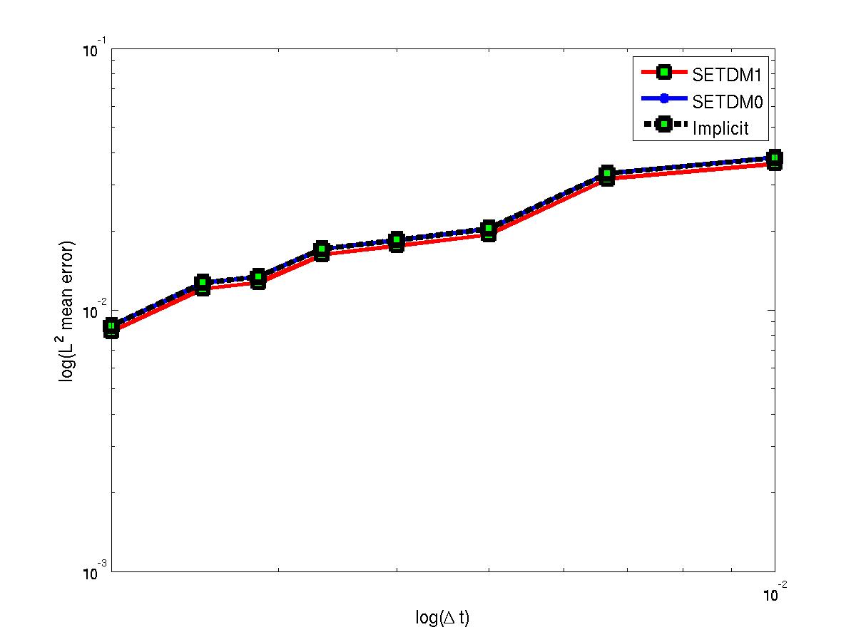
In the legends of our graphs, “SETDM1” denotes results from the SETDM1 scheme, “SETDM0 ” denotes results from the SETDM0 scheme with “Implicit” denotes results from the standard semi-implicit Euler-Maruyama scheme.

As a simple example consider the reaction diffusion equation with additive noise in the time interval $[0,T]$ with diffusion coefficient $D>0$

$$dX=(D\varDelta X-0.5X)dt+dW\;\;\;\;\;\;\;\;\;\;\;\;\;\;X(0)=X_{0},\;\;\;\;\;\;\Omega=[0,L_{1}]\times[0,L_{2}]\;\$$

with homogeneous Neumann boundary condition. As the exact solution is known for comparison, we take $f$ in the equation (2.5) to be linear here

$$f(u)=-0.5u.$$ (4.1)

The corresponding Nemytskii operator $F$ is obtained from (2.8). Of course, in general, $F$ will be nonlinear. $F$ verifies obviously Assumption 2.3. Here $b(x,u)=1,\;x\in\Omega,\;u\in\mathbb{R}$.

We consider the covariance operator $Q$ with the following covariance function (kernel) which has strong exponential decay

$$C_{r}((x_{1},y_{1});(x_{2},y_{2}))=\dfrac{\Gamma}{4b_{1}b_{2}}\exp\left(-\dfrac{\pi}{4}\left[\dfrac{\left(x_{2}-x_{1}\right)^{2}}{b_{1}^{2}}+\dfrac{\left(y_{2}-y_{1}\right)^{2}}{b_{2}^{2}}\right]\right),$$

where $b_{1},b_{2}$ are spatial correlation lengths in $x-$ axis and y- axis respectively and $\Gamma>0$.
It is well known that the eigenfunctions $\{e_{i}^{(1)}e_{j}^{(2)}\}_{i,j\geq 0}$ of the operator $A=D\varDelta$ is given by

$$\left\{\begin{array}[]{l}e_{0}^{(l)}=\sqrt{\dfrac{1}{L_{l}}},\;\;\;\lambda_{0}^{(l)}=0,\;\;\;e_{i}^{(l)}=\sqrt{\dfrac{2}{L_{l}}}\cos(\lambda_{i}^{(l)}x),\;\;\;\lambda_{i}^{(l)}=\dfrac{i\,\pi}{L_{l}}\\ \newline \\ l\in\left\{1,2\right\}\;\;\;i=1,2,3,\cdots\end{array}\right.$$ (4.5)

with the corresponding eigenvalues $\{\lambda_{i,j}\}_{i,j\geq 0}$ given by

$$\lambda_{i,j}=(\lambda_{i}^{(1)})^{2}+(\lambda_{j}^{(2)})^{2}.$$

The corresponding values of $\left\{q_{i,j}\right\}_{i+j>0}$ in the representation (1.2) are given by

$$q_{i,j}=\Gamma\exp\left[-\dfrac{1}{2\pi}\left((\lambda_{i}^{(1)}b_{1})^{2}+(\lambda_{j}^{(2)}b_{2})^{2}\right)\right],$$

see [23] for details and [25, 26]. We compute the exponential functions $\varphi_{i},\;i=0,1$ with the real fast Léja point technique and the absolute tolerance $10^{-6}$. In our simulation we take $L_{1}=L_{2}=1$ and the finite element triangulation is contructed with the rectangular grid with size $\Delta x=\Delta y=1/150$. Figure 1 shows the time convergence of SETDM1,SETDM0 and semi-implict schemes. The three methods have the same order of accuracy. The temporal order of convergence that we observe is $0.9$ for all the schemes. This is higher than the predicted theoretical order of comvergence $0.5$ in Theorem 2.7. The noise is regular and this order agrees with that in [22].

Figure 1: (a) Convergence of the root mean square $L^{2}$ norm at $T=1$ as a function of $\Delta t$ with 10 realizations with $X_{0}=0,\;\Gamma=1,\;D=1$. The noise is white in time and with exponential correlation in space with lengths $b_{1}=b_{2}=0.2$. The temporal order of convergence in time is $0.9$ for all schemes. In (b) we plot a sample true solution.

As a more challenging example we consider the stochastic advection diffusion reaction SPDE with multiplicative noise

$$dX = \left(\nabla\cdot\mathbf{D}\nabla X-\nabla\cdot(\mathbf{q}X)-\frac{X}{|X|+1}\right)dt+XdW,\qquad X_{0}=0\qquad\Omega=[0,1]\times[0,1]$$ (4.6)

$$\mathbf{D} = \left(\begin{array}[]{cc}10^{-2}&0\\ 0&10^{-3}\end{array}\right)$$ (4.9)

with mixed Neumann-Dirichlet boundary conditions. The Dirichlet boundary condition is $X=1$ at $x=0$ and we use the homogeneous Neumann boundary conditions elsewhere. According to Theorem 2.6, we need to take the initial data

$X_{0}\in L_{2}(\mathbb{D},\mathcal{D}((-A)^{\beta})),\;\beta>0$ to have a regular solution such that $XdW$ make sense. For our simulation we take $X_{0}=0$. For a homogeneous medium, we use the constant velocity $\mathbf{q}=(1,0)$. In terms of equation (2.5) the nonlinear terms $f$ and $b$ are given by

$$f(x,u)=-\frac{u}{(|u|+1)},\qquad b(x,u)=u,\quad u\in\mathbb{R},\;x\in\Omega,$$ (4.10)

and the corresponding Nemytskii operators $F$ and $B$ are obtained from (2.8) and clearly satisfy Assumption 2.3 (if the domain of $f$ is restricted to $\mathbb{R}^{+}$) and Assumption 2.4 (see [40, Section 4]) respectively, where (4.5) is used in the noise representation (1.2). The linear operator is given by

$$A=\nabla\cdot\mathbf{D}\nabla(.)-\nabla\cdot\mathbf{q}(.).$$ (4.11)

For a heterogeneous medium we used three parallel high permeability streaks. This could represent for example a highly idealized fracture pattern. We obtain the Darcy velocity field $\mathbf{q}$ by solving the system

$$\left\{\begin{array}[]{l}\nabla\cdot\mathbf{q}=0\\ \mathbf{q}=-\dfrac{k(\mathbf{x})}{\mu}\nabla p,\end{array}\right.$$ (4.14)

with Dirichlet boundary conditions $\Gamma_{D}^{1}=\left\{0,1\right\}\times\left[0,1\right]\text{and Neumann boundary}\quad\Gamma_{N}^{1}=\left(0,1\right)\times\left\{0,1\right\}$ such that

$$p = \left\{\begin{array}[]{l}1\quad\text{in}\quad\left\{0\right\}\times\left[0,1\right]\\ 0\quad\text{in}\quad\left\{1\right\}\times\left[0,1\right]\end{array}\right.$$

and

$$-k\,\nabla p(\mathbf{x},t)\,\cdot\mathbf{n}=0\quad\text{in}\quad\Gamma_{N}^{1},$$

where $p$ is the pressure, $\mu$ is dynamical viscosity and $k$ the permeability of the porous medium. We have assumed that rock and fluids are incompressible and sources or sinks are absent, thus the equation

$$\nabla\cdot\mathbf{q}=\nabla\cdot\left[\dfrac{k(\mathbf{x})}{\mu}\nabla p\right]=0$$ (4.16)

comes from mass conservation. As in [34, 32], we take the following values for $\left\{q_{i,j}\right\}_{i+j>0}$ in the representation (1.2)

$$q_{i,j}=1/\left(i+j\right)^{r},\qquad r>0.$$ (4.17)

Note that to have a trace class noise we need $r>2$. In our simulation we use $r=2.01$. To deal with high Péclet flows we discretize in space using finite volumes. We can write the semi-discrete finite volume discretization of (4.6) as

$$dX^{h}=(A_{h}X^{h}+P_{h}F(X^{h}))+P_{h}B(X^{h})dW,$$ (4.18)

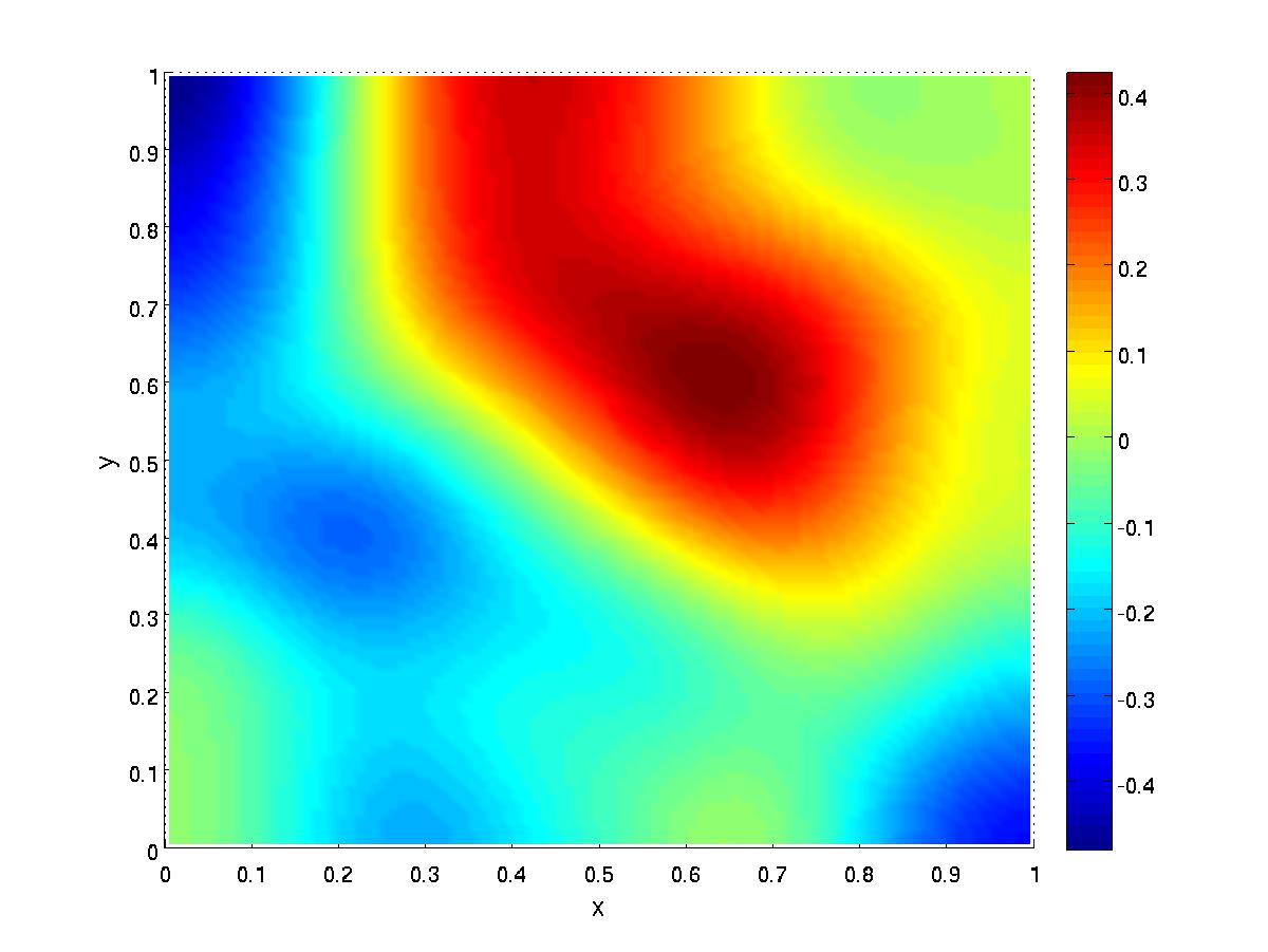
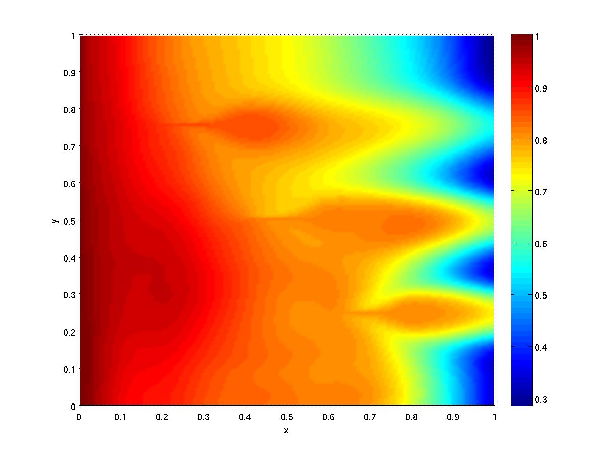
(see [33, 23]). Figure 2 shows the convergence of SETDM0, SETDM1 and semi-implicit schemes for the homogeneous porous medium. The scheme SETDM1 seems to be more accurate for large time steps but for large time steps it has the same order of accuracy as the semi-implicit and SETDM0 schemes. The temporal order is $0.54$ for SETDM1 scheme, $0.58$ for SETDM0 scheme and the semi-implicit scheme. We used 200 realizations and the convergence order is close to the $0.5$, the predicted order of convergence in Theorem 2.7. A sample the ’true solution’ is shown in Figure 2 with $\Delta t=1/1600$ while the mean of the ”true solution” for 200 realizations is shown in Figure 2.

Figure 2: (a) Convergence of the root mean square $L^{2}$ norm at $T=1$ as a function of $\Delta t$ with 200 realizations with $\Delta x=\Delta y=1/150$, $X_{0}=0$ for the homogeneous medium. The noise is white in time with (4.17) and $r=2.01$. The temporal orders of convergence in time are $0.54$ for SETDM1 and $0.58$ for SETDM0 semi-implicit schemes. In (b) we plot a sample of the ’true solution’ for $r=2.01$ with $\Delta t=1/1600$ while (c) shows the mean of the “true solution“ for 200 realizations.

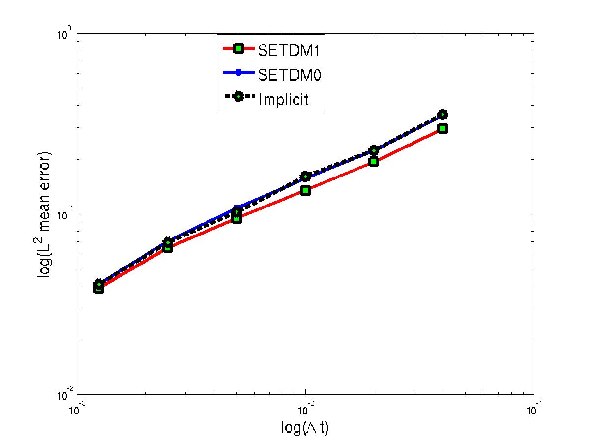
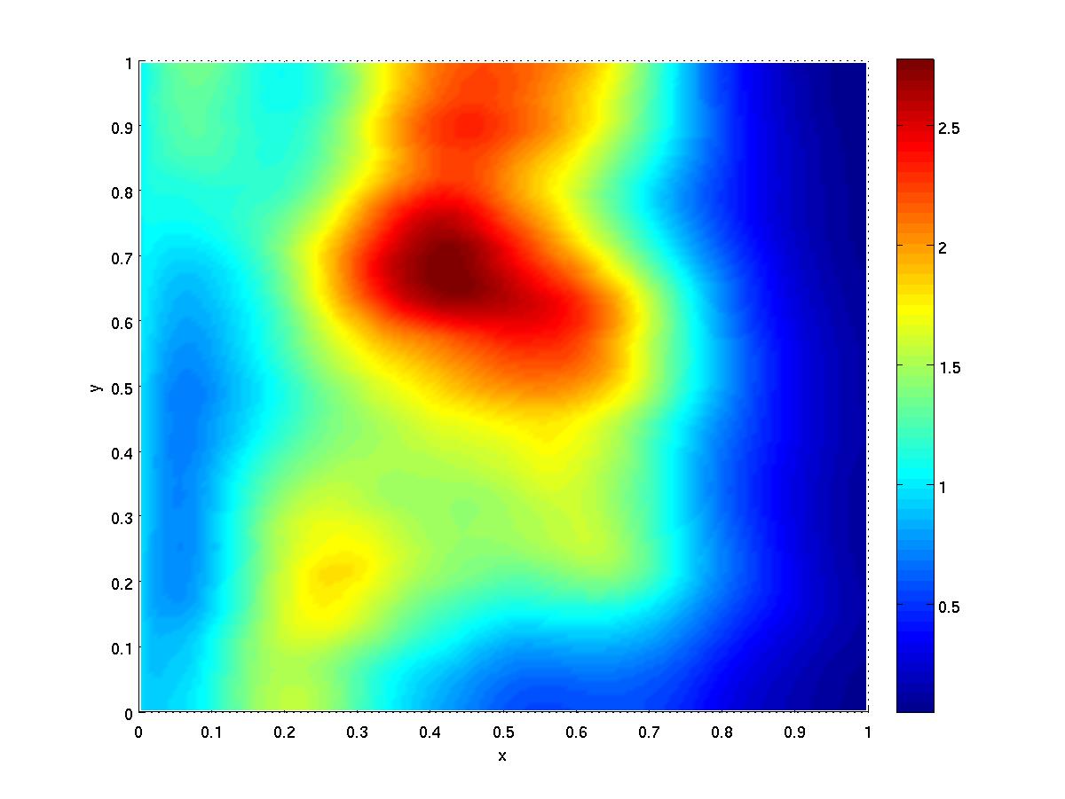
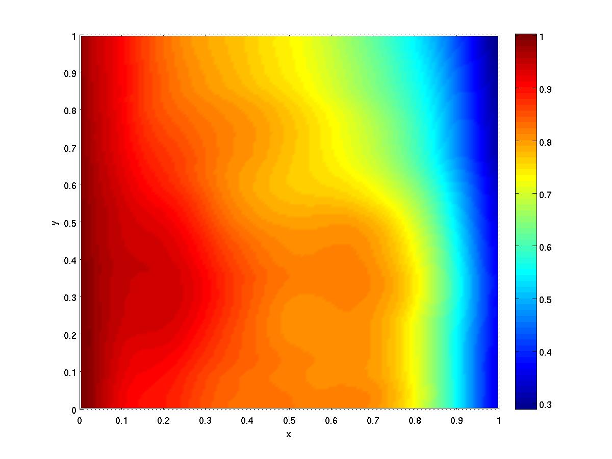
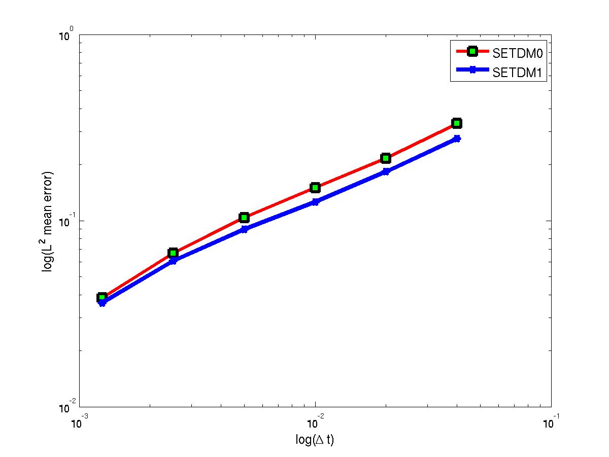
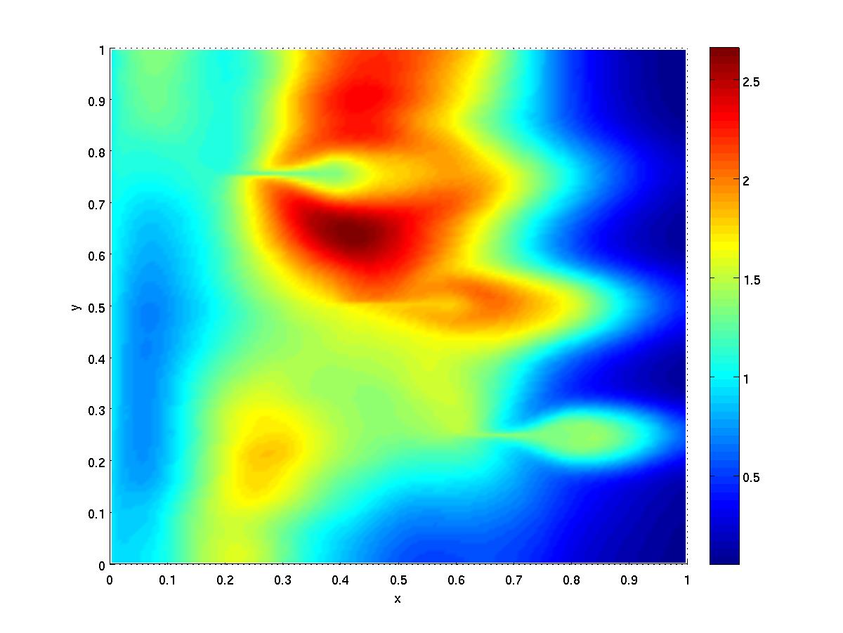
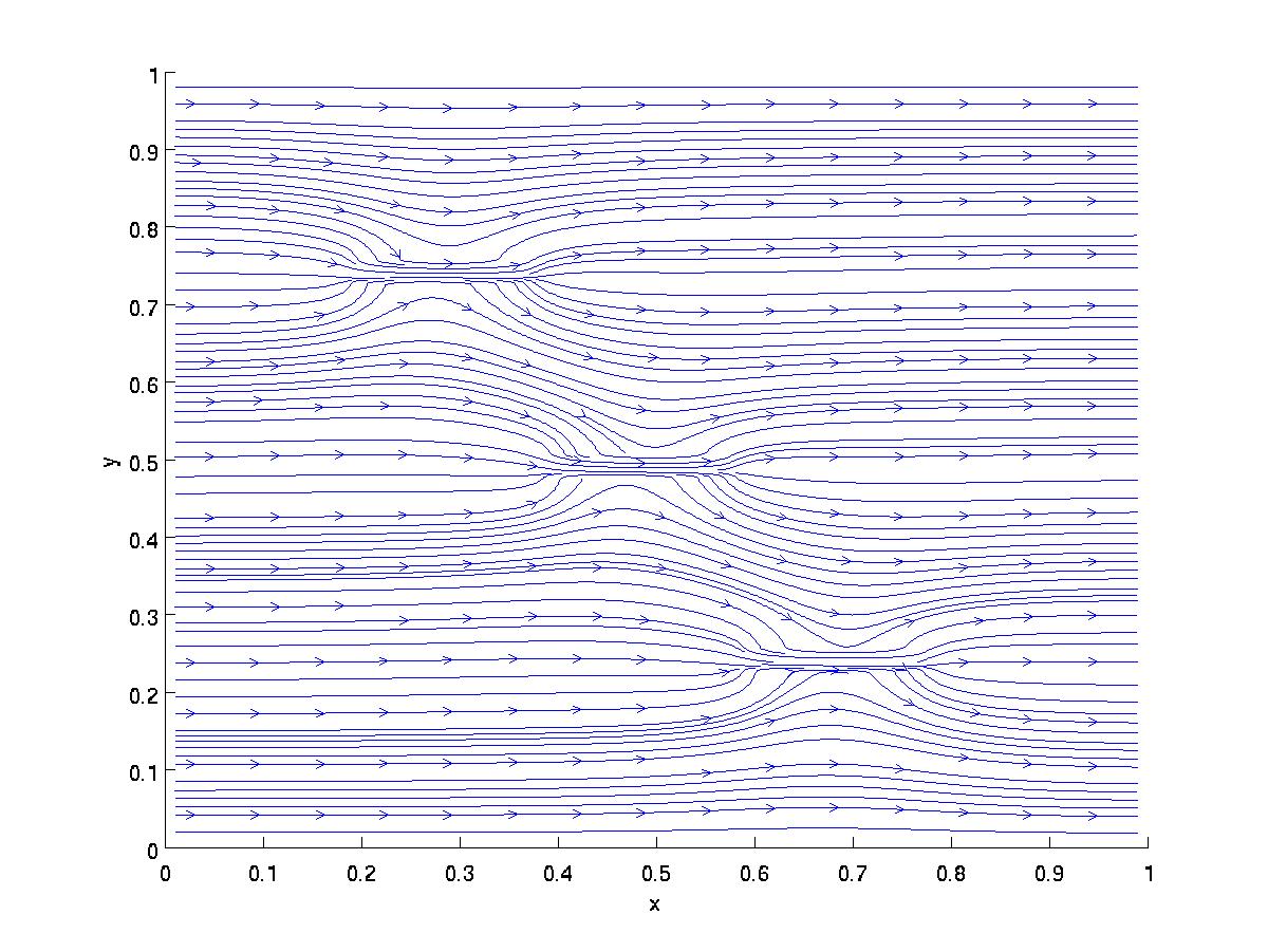
Figure 3 shows the convergence of SETDM0 and SETDM1 schemes for the heterogeneous porous medium. It also shows that SETDM1 is more accurate than SETDM0 scheme for high time step size. The observed temporal order is $0.54$ for SETDM1 scheme and $0.58$ for SETDM0 scheme. Figure 3 shows the streamline of the velocity field. A sample the “true solution“ is shown in Figure 3 with $\Delta t=1/1600$ while the mean of the ”true solution” for 200 realizations is shown in Figure 3.

To conclude we have proved the errors estimates for the exponential based integrators and observed the predicted rate of convergence in the simulations.

Figure 3: (a) Convergence of the root mean square $L^{2}$ norm at $T=1$ as a function of $\Delta t$ with 200 realizations with $\Delta x=\Delta y=1/150$, $X_{0}=0$ for the heterogeneous medium. The noise is white in time with (4.17) and $r=2.01$. The temporal orders of convergence in time are $0.54$ for SETDM1 scheme and $0.58$ for SETDM0. In (b) we plot a sample ’true solution’ for $r=2.01$ with $\Delta t=1/1600$. In (c) we plot the streamline of the velocity field while (d) shows the mean of the “true solution“ for 200 realizations.

References

- [1] G. Da Prato and J. Zabczyk. Stochastic Equations in Infinite Dimensions, volume 44 of Encyclopedia of Mathematics and its Applications. Cambridge University Press, Cambridge, 1992.
- [2] Claudia Prévôt and Michael Röckner. A Concise Course on Stochastic Partial Differential Equations. Springer, 2007. ISBN-10: 3540707808.
- [3] P-L. Chow. Stochastic Partial Differential Equations. Applied Mathematics and nonlinear Science. Chapman & Hall / CRC, 2007. ISBN-1-58488-443-6.
- [4] P. B. Bedient, H. S. Rifai, and C. J. Newell. Ground water contamination: Transport and remediation. Prentice Hall PTR , Englewood Cliffs, New Jersey 07632, 1994.
- [5] A. Jentzen. High order pathwise numerical approximations of SPDEs with additive noise. unpublished manuscript, 2009.
- [6] A. Jentzen. Pathwise numerical approximations of SPDEs . Potential Analysis, 31(4):375–404, 2009.
- [7] A. Jentzen and P. E. Kloeden. Overcoming the order barrier in the numerical approximation of SPDEs with additive space-time noise. Proc. R. Soc. A, 465(2102):649–667, 2009.
- [8] A. Jentzen, P. E. Kloeden, and G. Winkel. Efficient simulation of nonlinear parabolic SPDEs with additive noise. Annals of Applied Probability, In review, 2009.
- [9] G. J. Lord and A. Tambue. A modified semi–implict Euler-Maruyama scheme for finite element discretization of SPDEs. arXiv:1004.1998v1,2010.
- [10] G. J. Lord and A. Tambue. Stochastic Exponential Integrators for finite element discretization of SPDEs with Additive Noise. http://arxiv.org/abs/1005.5315, 2010.
- [11] C. Moler and C. Van Loan. Ninteen dubious ways to compute the exponential of a matrix, twenty–five years later. SIAM Review, 45(1), pp. 3–49, 2003.
- [12] M. Hochbruck and C. Lubich. On Krylov subspace approximations to the matrix exponential operator. SIAM J. Numer. Anal., 34(5), pp. 1911–1925., 1997.
- [13] R. B. Sidje. Expokit: A software package for computing matrix exponentials. ACM Trans. Math. Software, 24(1), pp.130–156, 1998.
- [14] A. Tambue, G. J. Lord, and S. Geiger. An exponential integrator for advection-dominated reactive transport in heterogeneous porous media. Journal of Computational Physics, 229(10):3957 – 3969, 2010.
- [15] M. Vianello, M. Caliari and L. Bergamaschi. Interpolating discrete advection diffusion propagators at Léja sequences. J. Comput. Appl. Math., 172(1), pp. 79–99, 2004.
- [16] D. Calvetti, J. Baglama and L. Reichel. Fast Léja points. Electron. Trans. Num. Anal., 7, pp.124–140, 1998.
- [17] M. Caliari, L. Bergamaschi and M. Vianello. The RELPM exponential integrator for FE discretizations of advection-diffusion equations. in: M. Bubak, G. D. Van Albada, P. Sloot (Eds.),Lecture Notes in Computer Sciences Volume 3039, Springer Verlag, Berlin Heidelberg, pp. 434-442, 2004.
- [18] D. Henry. Geometric theory of semilinear parabolic equations. Number 840 in Lecture notes in mathematics. Springer, 1981.
- [19] H. Fujita and T. Suzuki. Evolutions problems (part1). in: P. G. Ciarlet, J. L. Lions (Eds.) Handbook of Numerical Analysis, vol II, North-Holland, Amsterdam, pp. 789–928, 1991.
- [20] V.Thomée. Galerkin finite element methods for parabolic problems. Springer Series in Computational Mathematics, 1997.
- [21] B. Skaflestad H. Berland and W. Wright. A matlab package for exponential integrators. ACM Trans. Math. Software, 33(1), Article No. 4, 2007.
- [22] G. J. Lord and J. Rougemont. A numerical scheme for stochastic PDEs with Gevrey regularity. IMA J. Num. Anal.,24(4)(2004) 587–604 .
- [23] A. Tambue. Efficient Numerical Methods for Porous Media Flow. PhD thesis, Department of Mathematics, Heriot–Watt University, 2010.
- [24] I. B. Adamu. Numerical simulations of stochastic differential equations & the stochastic Swift-Hohenberg equation. . PhD thesis, Department of Mathematics, Heriot–Watt University, In preparation.
- [25] T. Shardlow. Numerical simulation of stochastic PDEs for excitable media. J. Comput. Appl. Math., 175(2):429–446, March 2005.
- [26] J. Garcí-Ojalvo and J. M. Sancho. Noise in spatially extended systems. Institute for Nonlinear Science. Springer-Verlag, New York, 1999.
- [27] Y. Yan. Semidiscrete Galerkin approximation for a linear stochastic parabolic partial differential equation driven by an additive noise. BIT, 44(4) (2004) 829–847.
- [28] Y. Yan. Galerkin Finite Element Methods for Stochastic Parabolic Partial Differential Equations. SIAM J. Num. Anal., 43(4) (2005) 1363–1384.
- [29] E. Hausenblas. Approximation for semilinear stochastic evolution equations. Potential Analysis, 18(2)(2003) 141–186.
- [30] E. J. Allen, and S. J. Novosel, and Z. Zhang. Finite element and difference approximation of some linear stochastic partial differential equations. Stochastics Stochastics Rep., 64(1-2)(1998) 117–142.
- [31] M. Kovács, S. Larsson, and F. Lindgren. Strong convergence of the finite element method with truncated noise for semilinear parabolic stochastic equations with additive noise. Numer. Algor. , 53 (2010) 309–320.
- [32] P. Kloeden, G. J. Lord, A. Neuenkirch and T. Shardlow. The exponential integrator scheme for stochastic partial differential equations: Pathwise error bounds. Accepted to J. Comp. A. Math., 2009.
- [33] R. Eymard, T. Gallouet, and R. Herbin, Finite volume methods, in: P. G. Ciarlet, J. L. Lions (Eds.), Handbook of Numerical Analysis Volume 7, North-Holland, Amsterdam, 2000, pp. 713–1020.
- [34] G. J. Lord and T. Shardlow. Postprocessing for stochastic parabolic partial differential equations. SIAM J. Numer. Anal., 45(2)(2007) 870–889.
- [35] D. J. Higham. An Algorithmic Introduction to Numerical Simulation of Stochastic Differential Equations. SIAM REVIEW , 43(3)(2001) 525–546.
- [36] S. Larsson. Nonsmooth data error estimates with applications to the study of the long-time behavior of finite element solutions of semilinear parabolic problems. Preprint 1992-36, Department of Mathematics, Chalmers University of Technology, available at http://www.math.chalmers.se/stig/papers/index.html .
- [37] C. M. Elliott and S. Larsson. Error estimates with smooth and nonsmooth data for a finite element method for the Cahn-Hilliard equation. Math. Comp. , 58 (1992) 603–630.
- [38] P. G. Ciarlet. The Finite Element Method for Elliptic Problems. North-Holland, 1978.
- [39] S. M. Cox and P. C. Matthews, Exponential time differencing for stiff systems, J. Comput. Phys. 176(2) (2002) 430–455.
- [40] A. Jentzen and M. Röckner. Regularity Analysis for Stochastic Partial Differential Equations with Nonlinear Multiplicative Trace Class Noise. http://arxiv.org/abs/1005.4095v1, 2010.
- [41] G. Da Prato and J. Zabczyk. Second Order Partial Differential Equations in Hilbert Spaces. London Mathematical Society, Lecture Notes, 293, Cambridge University Press, 2002.