Existence of a Center Manifold in a Practical Domain around $L_{1}$ in the Restricted Three Body Problem

Abstract

We give a proof of existence of centre manifolds within large domains for systems with an integral of motion. The proof is based on a combination of topological tools, normal forms and rigorous-computer-assisted computations. We apply our method to obtain an explicit region in which we prove existence of a center manifold in the planar Restricted Three Body Problem.

1 Introduction

Center manifolds are an important tool for the local analysis of dynamical systems. In this paper we develop a methodology to prove the existence of center manifolds in a “large” neighbourhood of the equilibrium point. The method involves the use of normal forms, topological results, and computer assisted computations. The novelty of our approach is that it provides explicit rigorous bounds on the size and location of the manifold for a given dynamical system. Moreover, under appropriate hypothesis we prove that the manifold is unique.

In contrast, the classical center manifold theorems show existence of a manifold in some neighbourhood, but they do not readily provide information on the size of this neighbourhood. Also, the classical normal form theorems construct an accurate approximation to the dynamics in a neighbourhood, but the normal form is usually not convergent. Sometimes the normal form does converge, but we lack information on its domain of convergence.

To show the power of our methodology, in the second part of this paper we prove existence and uniqueness of the center manifold in a practical domain around an equilibrium point of the celebrated Restricted Three Body Problem (RTBP). By practical we mean that such domain possibly could be used for realistic space mission design, since it is not too small. To our knowledge, this is the first proof of existence of the center manifold in a practical domain for the RTBP.

For the rest of this introduction, we define the center manifold and mention some previous results related to this paper. Finally we explain how this paper is organized into sections.

Definition 1.

Consider a differential equation on ${\mathbb{R}}^{n}$

$$\dot{x}=Ax+f(x),$$ (1)

where $A$ is linear and $f$ has no constant or linear terms. The origin is a fixed point. Let ${\mathbb{R}}^{n}=E^{c}\oplus E^{u}\oplus E^{s}$ be the usual decomposition into the center, unstable, and stable invariant subspaces with respect to $A$.

A center manifold $W^{c}$ is an invariant manifold of the flow of (1), tangent to $E^{c}$ at the origin, and of the form

$$W^{c}=\{(\theta,\chi(\theta))\colon\ \theta\in U\},$$

where $\chi\colon\ E^{c}\rightarrow E^{u}\oplus E^{s}$ is a $C^{k}$ function, and $U$ is an open neighborhood of $0$ in $E^{c}$.

We are naturally lead to study the flow in the center manifold. The center manifold approach has the advantage that this reduced problem is a dynamical system on a lower-dimensional manifold (of the same dimension as $E^{c}$). The reduced problem contains crucial information of the full problem (1). The qualitative behavior of the flow on the center manifold completely determines the behavior of the full flow around the fixed point [Car]. Also, every center manifold contains all globally bounded solutions (e.g. fixed points and periodic orbits) which are close enough to the origin [Sij].

Let us now mention some results related to this paper. The existence of center manifolds is discussed in many dynamical systems books, for instance in [GH, CH], and the monograph [Car]. The subtle properties of center manifolds such as (non)-uniqueness, tangency, limited differentiability, and (non)-analyticity are discussed in [Sij].

Lyapunov [L] studied the case in which the linear operator $A$ in equation (1) has a simple pair of eigenvalues $\pm\omega i$. He proved the existence of a center manifold filled with an analytic one-parameter family of periodic orbits. The main hypothesis are the presence of an integral of motion and a nonresonance condition. Such situation arises for the equilibrium point of the Restricted Three Body Problem that we study in the second part of this paper. Lyapunov’s theorem applies to the Restricted Three Body Problem (cf. [SM] §18), but again is only local and does not readily provide estimates on its domain of validity.

Normal forms make a very powerful and general technique to approximate local dynamics, including the center manifold, and stable/unstable manifolds of a fixed point. It is also a classical subject discussed in many dynamical system books, for instance [MH] (Hamiltonian systems), [CH] (general differential equations), [GH], and the monograph [Mu].

Given their usefulness, normal forms have been applied to approximate the center manifold around the equilibrium points of the planar Restricted Three Body Problem [CM, CDMR], and the spatial RTBP [JM, DMR]. In particular, our implementation of normal forms is based on [J]. This technique has important applications in space mission design [GJSM, GKLMMR] and diffusion estimates [JS, JV].

Regarding the planar RTBP, we would also like to mention the numerical explorations of Broucke [B], where he performed an extensive study of different families of periodic orbits. In particular, he finds a family of numerical periodic orbits around the same equilibrium point that we study in this paper. The family extends up to a very large neighborhood of the equilibrium point (much larger than our rigorous result).

The paper is organized as follows. In Section 2 we give the setup of the problem and state our main theorem (Theorem 5). Assumptions of the theorem are based on estimates on the derivatives of the vector field within the investigated region. Based on these the existence of an invariant manifold is established. In Section 3 we give a topological proof of the existence of an invariant manifold for maps with saddle-center-type properties. In Section 4 we use the result obtained for maps to prove Theorem 5. In Section 5 we apply our Theorem 5 to prove the existence of a center manifold around an equilibrium point $L_{1}$ in the RTBP. To do so we first introduce the problem and present a procedure of transforming the system into a normal form. We then discuss how normal forms provide very accurate approximations of center manifolds. Finally we combine Theorem 5 and normal forms with rigorous interval arithmetic based computer assisted computations to prove the existence of the manifold. Section 6 contains concluding remarks and an outline of future work.

2 Setup

We will consider the following problem. Let $F:\mathbb{R}^{n}\rightarrow\mathbb{R}^{n}$ and

$$\mathbf{x}^{\prime}=F(\mathbf{x})$$ (2)

be an ODE (we impose the usual assumptions implying existence and uniqueness of solutions) with a fixed point $\mathbf{x}_{0}$ and an integral of motion $H:\mathbb{R}^{n}\rightarrow\mathbb{R}$. By this we mean that for any solution $q(t)$ of (2) we have

$$H(q(t))=c,$$ (3)

where $c$ is some constants dependent on the initial condition $q(0)$. Since in our applications we shall deal with the restricted three body problem, which is a Hamiltonian system where $H$ is the Hamiltonian, we shall refer to $H$ as the energy from now on. We shall use a notation $\Phi(t,\mathbf{x})$ for the flow induced by (2).

2.1 Well aligned coordinates

We will investigate the dynamics of (2) in some compact set $D$, contained in an open subset $U$ of ${\mathbb{R}}^{n}$, such that the fixed point $\mathbf{x}_{0}\in D$, and whose image by a diffeomorphism

$$\phi:U\rightarrow\phi(U)\subset\mathbb{R}^{n}$$ (4)

is

$$\phi(D)=D_{\phi}=\bar{B}_{c}^{R}\times\bar{B}_{u}^{r}\times\bar{B}_{s}^{r},$$ (5)

where $\bar{B}_{i}^{r}$ (for $i\in\{c,u,s\}$) stand for $i$-dimensional closed balls around zero of radius $r$. We assume that $n=c+u+s$. We will refer to $p=\phi(\mathbf{x})$ as the aligned coordinates. In these coordinates we will use a notation $p=(\theta,x,y)$ with $\theta\in\bar{B}_{c}^{R},$ $x\in\bar{B}_{u}^{r}$ and $y\in\bar{B}_{s}^{r}$. We will refer to $\theta$ as the central coordinate, to $x$ as the unstable coordinate and to $y$ as the stable coordinate (the subscripts $c,u,s$ standing for central, unstable and stable respectively).

The motivation behind the above setup is the following. We will search for a center manifold of (2) homeomorphic to a $c$-dimensional disc inside the set $D$. Such manifolds have associated stable and unstable vector bundles, which in the coordinate system $\phi$ are given approximately by the coordinates of the balls $\bar{B}_{s}^{r}$ and $\bar{B}_{u}^{r}$ respectively. We do not assume though that the coordinates $x$ and $y$ align exactly with directions of hyperbolic expansion and contraction. It will turn out that it is enough that they point roughly in these directions. The remaining coordinates $\theta$ are the central coordinates of our system. We need to have a good guess on where the center manifold is. This guess is given by $\phi^{-1}(\bar{B}_{c}^{R}\times\{0\})\subset\mathbb{R}^{n}$. The change of coordinates $\phi$ can be obtained from some non-rigorous numerical computation (in our application for the RTBP - normal forms). It is important to emphasise that we will not assume that $\phi^{-1}(\bar{B}_{c}^{R}\times\{0\})$ is invariant under the flow (2). Allowing for errors, we expect the true manifold to lie in $\phi^{-1}(\bar{B}_{c}^{R}\times\bar{B}_{u}^{r}\times\bar{B}_{s}^{r}).$ This means that we take an enclosure of radius $r$ of our initial guess and look for the invariant manifold in this enclosure.

We will search for the part of the center manifold with energy $H\leq h$ for some $h\in\mathbb{R}$. We assume that the center coordinate is well aligned with the energy $H$ in the sense that we have

$$H(\phi^{-1}(\bar{B}_{c}^{R-v}\times\bar{B}_{u}^{r}\times\bar{B}_{s}^{r}))<h<H\left(\phi^{-1}(\partial\bar{B}_{c}^{R}\times\bar{B}_{u}^{r}\times\bar{B}_{s}^{r})\right),$$ (6)

for some $v>0$ (here we use a notation $\partial A$ to denote the boundary of a set $A$).

Our detection of the center manifold in the RTBP is going to be carried out in two stages. First we obtain $\phi$ as a change of coordinates into a normal form, after which we shall employ our topological theorem (Theorem 5) to prove the existence of the manifold.

2.2 Local bounds on the vector field and the statement of the main result

We are now ready to state the main assumptions needed for our method. These will be expressed in terms of local bounds on the derivative of the vector field (2). First let us introduce a notation $F^{\phi}$ for the vector field in the aligned coordinates i.e.

$$F^{\phi}(p)=D\phi(\phi^{-1}(p))F(\phi^{-1}(p)),$$ (7)

and a notation $[dF^{\phi}(N)]$ for an interval enclosure of the derivative on a set $N\subset D_{\phi}$

$$[dF^{\phi}(N)]=\left\{A\in\mathbb{R}^{n\times n}|A_{ij}\in\left[\inf_{p\in N}\frac{dF_{i}^{\phi}}{dp_{j}},\sup_{p\in N}\frac{dF_{i}^{\phi}}{dp_{j}}\right],\text{ for all }i,j=1,\ldots,n\right\}.$$

For any point $p=(\theta,0,0)$ from $\bar{B}_{c}^{R}\times\{0\}\times\{0\}$ we define a set

$$N_{p}:=\bar{B}_{c}(\theta,\rho)\times\bar{B}_{u}^{r}\times\bar{B}_{s}^{r}\cap D_{\phi},$$ (8)

where $\bar{B}_{c}(\theta,\rho)$ is a $c$ dimensional ball of radius $\rho>0\$centred at $\theta$. We introduce the following notations for the bound on the derivatives of $F^{\phi}$ on the sets $N_{p}$

$$[dF^{\phi}(N_{p})]\subset\left(\begin{array}[c]{ccc}\mathbf{C}&\boldsymbol{\varepsilon}_{c}&\boldsymbol{\varepsilon}_{c}\\ \boldsymbol{\varepsilon}_{m}&\mathbf{A}&\boldsymbol{\varepsilon}_{u}\\ \boldsymbol{\varepsilon}_{m}&\boldsymbol{\varepsilon}_{s}&\mathbf{B}\end{array}\right).$$ (9)

Here $\mathbf{A,B,C,}\boldsymbol{\varepsilon}_{c},\boldsymbol{\varepsilon}_{m},\boldsymbol{\varepsilon}_{s}$ and $\boldsymbol{\varepsilon}_{u}$ are interval matrices, that is matrices with interval coefficients. Here we slightly abuse notations since the pairs of matrices $\boldsymbol{\varepsilon}_{c}$ and $\boldsymbol{\varepsilon}_{m}$ need not be equal; they even have different dimension when $u\neq s$. We use the same notation since later on we shall assume uniform bounds for both of matrices $\boldsymbol{\varepsilon}_{c}$ and both $\boldsymbol{\varepsilon}_{m}$. Let us also note that the bounds $\mathbf{A,B,C,}\boldsymbol{\varepsilon}_{c},\boldsymbol{\varepsilon}_{m},\boldsymbol{\varepsilon}_{s}$ and $\boldsymbol{\varepsilon}_{u}$ may be different for different $p.$ We do not indicate this in our notations to keep them relatively simple.

Remark 2.

If the system possesses a center manifold and the adjusted coordinates are well aligned in the sense of section 2.1, then the interval matrices $\boldsymbol{\varepsilon}_{i}$ in (9), with $i\in\{c,m,s,u\}$ should turn out to be small. The matrices $\mathbf{A,B,C}$ are the bounds on derivatives of the vector field in the unstable, stable and central directions respectively. If the alignment of our coordinates is correct then we expect the contraction/expansion rates associated with $\mathbf{C}$ to be weaker than for $\mathbf{A}$ and $\mathbf{B.}$

We will use the following notations to express our assumptions about $[dF^{\phi}(N_{p})].$ Let $\delta^{u},\delta^{s},c^{u},c^{s},\varepsilon_{i}>0$ denote contraction/expansion rates, such that for any matrix $A\in\mathbf{A}$, $B\in\mathbf{B,}$ $e_{i}\in\boldsymbol{\varepsilon}_{i}$ for $i\in\{m,c,u,s\}$, we have

$$\inf\{x^{T}Ax:||x||=1\}>\delta^{u},$$ (10)

$$\sup\{y^{T}By:||y||=1\}<-\delta^{s},$$ (11)

$$c^{s}<\inf\{\theta^{T}C\theta:||\theta||=1\}\leq\sup\{\theta^{T}C\theta:||\theta||=1\}<c^{u},$$ (12)

$$||e_{i}||<\varepsilon_{i}\quad\text{for }i\in\{m,c,u,s\}.$$ (13)

Once again, $\varepsilon_{i},c^{s},c^{u},\mu,\delta^{u}$ and $\delta^{s}$ can depend on $p$.

Let $\gamma,\alpha_{h},\alpha_{v},\beta_{h},\beta_{v}>0$ be constants such that

$$\alpha_{h}>\alpha_{v}\quad\text{and}\quad\beta_{v}>\beta_{h},$$ (14)

and such that the radius $\rho$ considered for the central part of the sets $N_{p}$ satisfies

$$\rho>r\sqrt{\frac{\alpha_{h}}{\gamma}},\quad\quad\rho>r\sqrt{\frac{\beta_{v}}{\gamma}},\qquad$$ (15)

where $r$ is the radius of the balls $\bar{B}_{u}^{r}$ and $\bar{B}_{s}^{r}$ in (5). Let us define the following constants

$$\kappa_{c}^{\text{forw}} :=c^{u}+\frac{1}{2}\left(\frac{\alpha_{h}}{\gamma}\varepsilon_{m}+\frac{\beta_{h}}{\gamma}\varepsilon_{m}+2\varepsilon_{c}\right),$$

$$\kappa_{u}^{\text{forw}} :=\delta^{u}-\frac{1}{2}\left(\varepsilon_{m}+\varepsilon_{u}+\frac{\gamma}{\alpha_{h}}\varepsilon_{c}+\frac{\beta_{h}}{\alpha_{h}}\varepsilon_{s}\right),$$ (16)

$$\kappa_{s}^{\text{forw}} :=-\delta^{s}+\frac{1}{2}\left(\varepsilon_{m}+\frac{\alpha_{h}}{\beta_{h}}\varepsilon_{u}+\frac{\gamma}{\beta_{h}}\varepsilon_{c}+\varepsilon_{s}\right),$$

$$\kappa_{c}^{\text{back}} :=c^{s}-\frac{1}{2}\left(\varepsilon_{m}\frac{\alpha_{v}}{\gamma}+\varepsilon_{m}\frac{\beta_{v}}{\gamma}+2\varepsilon_{c}\right),$$

$$\kappa_{u}^{\text{back}} :=\delta^{u}-\frac{1}{2}\left(\varepsilon_{m}+\varepsilon_{u}+\frac{\gamma}{\alpha_{v}}\varepsilon_{c}+\frac{\beta_{v}}{\alpha_{v}}\varepsilon_{s}\right),$$ (17)

$$\kappa_{s}^{\text{back}} :=-\delta^{s}+\frac{1}{2}\left(\varepsilon_{m}+\frac{\alpha_{v}}{\beta_{v}}\varepsilon_{u}+\frac{\gamma}{\beta_{v}}\varepsilon_{c}+\varepsilon_{s}\right).$$

The superscripts ”forw” and ”back” in the above constants come from the fact that they shall be associated with estimates on the dynamics induced by the vector field (7), for forward and backward evolution in time respectively. At this stage the subscripts $v$ and $h$ in constants $\alpha$ and $\beta$ do not have an intuitive meaning. During the course of the proof they shall be associated with horizontal and vertical slopes of constructed invariant manifolds (hence $h$ for ”horizontal” and $v$ for ”vertical”), and then their meaning will become more natural.

Remark 3.

Even though coefficients (16), (17) are technical in nature, they have a quite natural interpretation in terms of the dynamics of the system. The estimates $\kappa_{c}^{i},\kappa_{u}^{i},\kappa_{s}^{i}$ for $i\in\{$forw,back$\}$ are essentially estimates on the contraction/expansion rates associated with the center, unstable and stable coordinates respectively. These estimates take into account errors $\varepsilon_{i}$ for $i\in\{s,u,c,m\}$ in the setup of coordinates. Note that when our coordinates are perfectly aligned with the dynamics, then $\varepsilon_{i}=0$ for $i\in\{s,u,c,m\},$ and in turn

$$\kappa_{s}^{\text{forw}}=\kappa_{s}^{\text{back}}=-\delta^{s},\quad\quad\kappa_{c}^{\text{back}}=c^{s},\quad\quad\kappa_{c}^{\text{forw}}=c^{u},\quad\quad\kappa_{u}^{\text{forw}}=\kappa_{u}^{\text{back}}=\delta^{u},$$

which are the bounds on the derivative of the vector field in the unstable, stable and center directions given in (10), (11), (12). The key assumptions of Theorem 5 are (18) and (19). In particular, these assumptions imply

$$\kappa_{s}^{\text{back}}<\kappa_{c}^{\text{back}}\quad\quad\kappa_{c}^{\text{forw}}<\kappa_{u}^{\text{forw}},$$

which is equivalent to assuming that the dynamics in the center coordinate is weaker than dynamics in the stable and unstable directions. These are classical assumptions for center manifold theorems (See [GH], for instance).

Remark 4.

We have certain freedom of choice for the constants $\gamma$, $\alpha_{h}$, $\alpha_{v}$, $\beta_{h}$, $\beta_{v}$. They offer flexibility when verifying assumptions of Theorem 5. During the course of the proof of Theorem 5 it will turn out that they also give Lipschitz type bounds $L_{c}=\sqrt{\frac{2\gamma}{\min(\alpha_{h}-\alpha_{v},\beta_{v}-\beta_{h})}},$ $L_{s}=\sqrt{\frac{1}{\alpha_{h}}\max(\gamma,\beta_{h})},$ $L_{u}=\sqrt{\frac{1}{\beta_{v}}\max(\gamma,\alpha_{v})}$ for our center, stable and unstable manifolds respectively (for more details see Corollary 20).

We are now ready to state our main tool for detection of center manifolds.

Theorem 5.

(Main Theorem) Let $h\in\mathbb{R}.$ Assume that (6) holds for some $v>0.$ Assume also that for any $p\in\bar{B}_{c}^{R}\times\{0\}\times\{0\},$ for the constants $\kappa_{c}^{\text{forw}}$, $\kappa_{u}^{\text{forw}}$, $\kappa_{s}^{\text{forw}}$, $\kappa_{c}^{\text{back}}$, $\kappa_{u}^{\text{back}}$, $\kappa_{s}^{\text{back}}$, $\varepsilon_{u}$, $\varepsilon_{s}$, $\delta^{u}$, $\delta^{s}$ computed on a set $N_{p}$ (defined by (8)) the following inequalities hold:

$$\kappa_{c}^{\text{forw}},\kappa_{s}^{\text{forw}} <\kappa_{u}^{\text{forw}},\hskip 56.9055pt0<\kappa_{u}^{\text{forw}},$$ (18)

$$\kappa_{s}^{\text{back}} <0,\hskip 56.9055pt\kappa_{s}^{\text{back}}<\kappa_{c}^{\text{back}},\kappa_{u}^{\text{back}},$$ (19)

and also that there exist $E_{u},E_{s}>0$ such that for any $q\in N_{p}\cap(\bar{B}_{c}^{R}\times\{0\}\times\{0\})$

$$||\pi_{x}F^{\phi}(q)||<rE_{u},\quad\text{\quad}||\pi_{y}F^{\phi}(q)||<rE_{s},$$ (20)

and

$$E_{u}+\varepsilon_{u} <\delta^{u},$$ (21)

$$E_{s}+\varepsilon_{s} <\delta^{s}.$$ (22)

If above assumptions hold, then there exists a $C^{0}$ function

$$\chi:\bar{B}_{c}^{R-v}\rightarrow D_{\phi}$$

such that

1. For any $\theta\in\bar{B}_{c}^{R-v}$ we have $\pi_{\theta}\chi(\theta)=\theta$ and

   $$\Phi(t,\phi^{-1}(\chi(\theta)))\in D\quad\text{for all }t\in\mathbb{R}.$$

2. If for some $\mathbf{x}\in\phi^{-1}(\bar{B}_{c}^{R-v}\times\bar{B}_{u}^{r}\times\bar{B}_{s}^{r})$ we have

   $$\Phi(t,\mathbf{x})\in D\quad\text{for all }t\in\mathbb{R}$$

   then there exists a $\theta\in\bar{B}_{c}^{R-v}$ such that $\mathbf{x}=\phi^{-1}(\chi(\theta))$.

In subsequent sections we shall present a proof of this theorem building up auxiliary results along the way. Before we move on to these results let us make a couple of comments on the result.

Remark 6.

Theorem 5 establishes uniqueness of the invariant manifold. This is not a typical scenario in case of center manifolds which are usually not unique. Uniqueness in our case follows from condition (6), which by our construction will ensure that for any point from our center manifold a trajectory starting from it cannot leave the set $D$. This means that dynamics on the center manifold with $H\leq h$ is contained in a compact set. This is the underlying reason that allows us to obtain uniqueness.

Remark 7.

The main strength of our result lies in the fact that it allows us to easily obtain explicit bounds for the position and size of the manifold. The center manifold is contained in $D=\phi^{-1}(\bar{B}_{c}^{R}\times\bar{B}_{u}^{r}\times\bar{B}_{s}^{r})$. Since the manifold is a graph of $\chi,$ from point 1. of Theorem 5 we know that it is of the form $\phi^{-1}\left\{\left(\theta,\pi_{x,y}\chi(\theta)\right)|\theta\in\bar{B}_{c}^{R-v}\right\},$ which ensures that it ”fills in” the set $D$ nontrivially. In contrast, the classical center manifold theorem does not provide such explicit bounds.

Remark 8.

In principle, one could derive some explicit analytic bounds using e.g. the “method of majorands” explained in the book of Siegel–Moser [SM]. However, to guarantee existence of the center manifold in a neighborhood of the equilibrium point that is not too small, one would require a substantial amount of very careful estimates.

Remark 9.

It is important to remark that our result only establishes continuity (together with Lipschitz type conditions) of the center manifold. The center manifold theorem clearly indicates that in a sufficiently small neighbourhoods of a saddle-center fixed point we should have higher order smoothness. We believe though that similar in spirit assumptions to those of Theorem 5 should imply higher order smoothness. This will be the subject of forthcoming work. The result obtained so far should be regarded as a first step towards this end.

In our application for the RTBP, in a neighbourhood sufficiently close to the equilibrium point, our manifold shall inherit all regularity which follows from the center manifold theorem (see Remark 21).

Let us finish the section with a final comment. In order to verify assumptions of Theorem 5 it is sufficient to consider some finite covering $\{\bigcup_{i\in I}U_{i}\}$ of the set $D_{\phi}$ and to verify bounds on local derivatives on sets $U_{i}.$ It is not necessary to consider an infinite number of points $p$ and their associated sets $N_{p},$ as long as for any $p\in\bar{B}_{c}^{R}\times\{0\}\times\{0\}$ we have $N_{p}\subset U_{i}$ for some $i\in I.$ This makes assumptions of Theorem 5 verifiable in practice using rigorous computer assisted tools.

3 Topological approach to centre manifolds for maps

In this section we will state some preliminary results, which will next be used for the proof of Theorem 5 in Section 4. The results will be stated for maps instead of flows. In Section 4 we will take a time shift along a trajectory map for the flow generated by (2) and apply the results to it. The main result of this section is Theorem 16. The result is in the spirit of versions of normally hyperbolic invariant manifold theorems obtained in [Ca], [CZ] and [CS]. The main difference is that we do not deal with a normally hyperbolic manifold without boundary, but with a selected part of a centre manifold (homeomorphic to a disc) with a boundary. In this section the fact that the dynamics does not diffuse through the boundary along the centre coordinate is imposed by assumption. This assumption will later follow from assuming that (3), (6) hold for (2).

We now give the setup for maps. Let $D\subset U\subset\mathbb{R}^{n}$, the change of coordinates $\phi:U\rightarrow\phi(U)$, and $D_{\phi}=\phi(D)$, be as in Section 2.1. We consider a dynamical system given by a smooth invertible map $f:U\rightarrow U.$ In adjusted coordinates we denote the map as $f_{\phi}:=\phi\circ f\circ\phi^{-1}$, $f_{\phi}:\phi(U)\rightarrow\mathbb{R}^{n}.$ We assume that

$$H(p)=H(f(p))$$ (23)

for all $p\in D_{\phi}$ and also that for some $v>0$ condition (6) holds.

We introduce the following sets

$$D_{\phi}^{-} =\bar{B}_{c}^{R}\times\partial\bar{B}_{u}^{r}\times\bar{B}_{s}^{r},$$ (24)

$$D_{\phi}^{+} =\bar{B}_{c}^{R}\times\bar{B}_{u}^{r}\times\partial\bar{B}_{s}^{r}.$$

We now introduce a number of definitions. The first is a definition of a covering relation.

Fig. 1: A map $f$ which satisfies covering conditions. The set $D_{\phi}$ is contracted in coordinate $y$ and expanded in coordinate $x$. Note that in the $\theta$ coordinate the set may be simply shifted, expanded or contracted, just as long as conditions (25),…,(29) are satisfied.

Definition 10.

We say that a map $f:U\rightarrow U$ satisfies covering conditions in $D$ if

$$\pi_{x}(f_{\phi}(D_{\phi}^{-}))\cap\bar{B}_{u}^{r} =\emptyset,$$ (25)

$$\pi_{y}(f_{\phi}^{-1}(D_{\phi}^{+}))\cap\bar{B}_{s}^{r} =\emptyset,$$ (26)

$$\pi_{y}(f_{\phi}(D_{\phi}))\cap\left(\mathbb{R}^{s}\setminus\bar{B}_{s}^{r}\right) =\emptyset,$$ (27)

$$\pi_{x}(f_{\phi}^{-1}(D_{\phi}))\cap\left(\mathbb{R}^{u}\setminus\bar{B}_{u}^{r}\right) =\emptyset,$$ (28)

and for any point $p\in\bar{B}_{c}^{R}\times\{0\}$,

$$\pi_{(x,y)}f_{\phi}(p),\,\pi_{(x,y)}f_{\phi}^{-1}(p)\in\mathrm{int}\left(\bar{B}_{u}^{r}\times\bar{B}_{s}^{r}\right).$$ (29)

Conditions (27) and (26) mean that, in the $y$ (stable) projection, $f_{\phi}$ contracts the set $D_{\phi}$ strictly inside $\bar{B}_{s}^{r}$. Conditions (28) and (25) mean that, in the $x$ (unstable) projection, $f_{\phi}$ expands the set $D_{\phi}$ strictly outside $\bar{B}_{s}^{r}$. The final assumption (29) is needed to ensure that the image of $D_{\phi}$ by $f_{\phi}$ intersects $D_{\phi}$. Without assumption (29), all other assumptions (25),…,(28) could easily follow from having image of $D$ disjoint with $D$.

Covering relations are tools which can be used to ensure existence of an invariant set in $D$. To prove that this set is a manifold we shall need additional assumptions. These shall be expressed by “cone conditions”. To introduce these conditions, first we need some notations.

Let $Q_{h},Q_{v}:\mathbb{R}^{c}\times\mathbb{R}^{s}\times\mathbb{R}^{u}\rightarrow\mathbb{R}$ be functions defined by

$$Q_{h}(\theta,x,y) =-\gamma||\theta||^{2}+\alpha_{h}||x||^{2}-\beta_{h}||y||^{2},$$ (30)

$$Q_{v}(\theta,x,y) =-\gamma||\theta||^{2}-\alpha_{v}||x||^{2}+\beta_{v}||y||^{2},$$

with $\gamma,\alpha_{h},\alpha_{v},\beta_{h},\beta_{v}>0$ and

$$\alpha_{h}>\alpha_{v}\quad\text{and}\quad\beta_{v}>\beta_{h}.$$ (31)

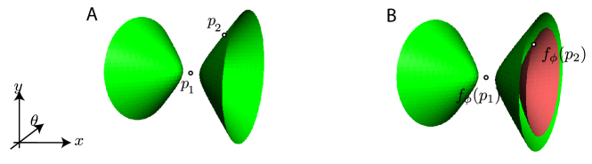
Fig. 2: An example of a function $f$, which satisfies cone conditions: A. Two points $p_{1},p_{2}$ for which $Q_{h}(p_{1}-p_{2})=c>0$. B. Difference of the images of the points lie on a cone $Q_{h}(f_{\phi}(p_{1})-f_{\phi}(p_{2}))>mc$. Similar condition (but with reversed roles of the $x$ and $y$ coordinates) needs to hold for the inverse map.

Definition 11.

We say that a map $f:U\rightarrow U$ satisfies cone conditions in $D$ if there exists an $m>1$ such that

1. for any two points $p_{1},p_{2}\in D_{\phi}$ satisfying $p_{1}\neq p_{2}$ and $Q_{h}(p_{1}-p_{2})\geq 0$ we have

   $$Q_{h}(f_{\phi}(p_{1})-f_{\phi}(p_{2}))>mQ_{h}(p_{1}-p_{2}),$$ (32)

2. for any two points $p_{1},p_{2}\in D_{\phi}$ satisfying $p_{1}\neq p_{2}$ and $Q_{v}(p_{1}-p_{2})\geq 0$ we have

   $$Q_{v}(f_{\phi}^{-1}(p_{1})-f_{\phi}^{-1}(p_{2}))>mQ_{v}(p_{1}-p_{2}).$$ (33)

Definition 11 intuitively states that if we have two points that lie horizontally with respect to each other, then their images are going to be pulled apart in the horizontal, $x$ coordinate (see Figure 2). If on the other have we have two points that lie vertically with respect to each other, then their pre-images are going to be pulled apart in the vertical, $y$ coordinate.

We now give definitions of horizontal discs and vertical discs. These will be building blocks in our construction of invariant manifolds.

Definition 12.

We say that a continuous monomorphism $\mathbf{h}:\bar{B}_{u}^{r}\rightarrow D_{\phi}$ is a horizontal disc if $\pi_{x}\mathbf{h}(x)=x$ and for any $x_{1},x_{2}\in\bar{B}_{u}^{r}$

$$Q_{h}(\mathbf{h}(x_{1})-\mathbf{h}(x_{2}))\geq 0.$$ (34)

Thus, to any point $x$ in the graph $\mathbf{h}(x)$ we can attach a horizontal cone, so that the graph always remains entirely inside the cone (see Figure 3).

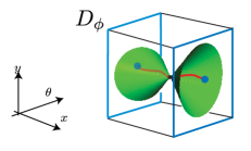
Fig. 3: A horizontal disc in $D_{\phi}$.

Definition 13.

We say that a continuous monomorphism $\mathbf{v}:\bar{B}_{s}^{r}\rightarrow D_{\phi}$ is a vertical disc if $\pi_{y}\mathbf{v}(y)=y$ and for any $y_{1},y_{2}\in\bar{B}_{s}^{r}$

$$Q_{v}(\mathbf{v}(y_{1})-\mathbf{v}(y_{2}))\geq 0.$$

Thus, to any point $y$ in the graph $\mathbf{v}(y)$ we can attach a vertical cone, so that the graph always remains entirely inside the cone.

The following lemma is a key auxiliary result for the proof of Theorem 16, which is the main result of this section. Roughly speaking, it states that under appropriate conditions, an image of a horizontal disc is a horizontal disc.

Lemma 14.

Let $\mathbf{h}_{1}$ be a horizontal disc. If $f$ satisfies covering and cone conditions in $D$, then there exists a horizontal disc $\mathbf{h}_{2}$ such that

$$\{p:\pi_{x,y}p\in\bar{B}_{u}^{r}\times\bar{B}_{s}^{r}\}\cap f_{\phi}(\mathbf{h}_{1}(\bar{B}_{u}^{r}))=\mathbf{h}_{2}(\bar{B}_{u}^{r}).$$

Moreover, if $H(\phi^{-1}(\mathbf{h}_{1}(\bar{B}_{u}^{r})))<h$, and for any $p\in D_{\phi}$ such that $H(\phi^{-1}(p))<h$ we have

$$\pi_{\theta}(f_{\phi}(p))\in\bar{B}_{c}^{R},$$ (35)

then

$$\mathbf{h}_{2}(\bar{B}_{u}^{r})\subset D_{\phi}\quad\text{and\quad}H(\phi^{-1}(\mathbf{h}_{2}(\bar{B}_{u}^{r})))<h.$$

Proof.

Without loss of generality we can assume that $\phi$ is equal to identity. Thus we can set $D_{\phi}=D$ and $f_{\phi}=f$.

Let $\mathbf{h}$ be any horizontal disc, then by (30), (34) and (32) for $x_{1}\neq x_{2}$

$$\alpha_{h}\left\|\pi_{x}f(\mathbf{h}(x_{1}))-\pi_{x}f(\mathbf{h}(x_{2}))\right\|^{2} \geq Q_{h}(f(\mathbf{h}(x_{1}))-f(\mathbf{h}(x_{2})))$$ (36)

$$>mQ_{h}(\mathbf{h}(x_{1})-\mathbf{h}(x_{2}))$$

$$\geq 0,$$

which means that $\pi_{x}\circ f\circ\mathbf{h}$ is injective.

Let us define a function $F:\bar{B}_{u}^{r}\rightarrow\mathbb{R}^{u}$ as follows

$$F(x):=\pi_{x}(f(\mathbf{h}_{1}(x))).$$

We shall first show that there exists an $x_{0}\in\bar{B}_{u}$ such that $F(x_{0})\in\bar{B}_{u}^{r}$. Using notations $\mathbf{h}_{1}(x)=(h_{\theta}(x),x,h_{y}(x))$ we can define a family of horizontal discs $\mathbf{h}_{\alpha}(x)=(\alpha h_{\theta}(x),x,\alpha h_{y}(x)).$ We define a function $l:[0,1]\times\bar{B}_{u}^{r}\rightarrow\mathbb{R}^{u}$ as

$$l(\alpha,x):=\pi_{x}\circ f\circ\mathbf{h}_{\alpha}(x).$$

By (24) and (25), since $\mathbf{h}_{\alpha}(\partial\bar{B}_{u}^{r})\subset D^{-},$ for any $\alpha\in[0,1]$ we have $l(\alpha,\partial\bar{B}_{u}^{r})\cap\bar{B}_{u}^{r}=\emptyset.$ Since, as shown at the beginning of the proof,

$$l(\alpha,\cdot):=\pi_{x}\circ f\circ\mathbf{h}_{\alpha}:\bar{B}_{u}^{r}\rightarrow\mathbb{R}^{u}$$

is a continuous monomorphism, we either have $l(\alpha,\bar{B}_{u}^{r})\cap\bar{B}_{u}^{r}=\emptyset$ or $\bar{B}_{u}^{r}\subset\mathrm{int}(l(\alpha,\bar{B}_{u}^{r})).$ This also means that

$$\inf\{\left\|l(\alpha,0)-x\right\|:x\in\partial\bar{B}_{u}^{r}\}>0,$$

and thus the function $\delta:[0,1]\rightarrow\mathbb{R}$ defined as

$$\delta(\alpha):=\left\{\begin{array}[c]{lll}0&&l(\alpha,0)\in\bar{B}_{u}^{r}\\ 1&&l(\alpha,0)\notin\bar{B}_{u}^{r},\end{array}\right.$$

is continuous. We have

$$\pi_{x}\mathbf{h}_{\alpha=0}(0) =0,$$

$$\pi_{y}\mathbf{h}_{\alpha=0}(0) =0,$$

so condition (29) implies $l(0,0)=\pi_{x}\circ f(\mathbf{h}_{\alpha=0}(0))\in B_{u}^{r},$ hence $\delta(0)=0.$ Suppose, to obtain a contradiction, that $F(x)\notin\bar{B}_{u}^{r}$ for all $x\in\bar{B}_{u}^{r}$. This would mean that in particular $F(0)=l(1,0)\notin\bar{B}_{u}^{r}$, hence $\delta(1)=1.$ This contradicts the fact that $\delta(0)=0$ and $\delta$ is continuous.

We have shown that there exists an $x_{0}\in\bar{B}_{u}^{r}$ such that $F(x_{0})\in\bar{B}_{u}^{r}.$ From (25) follows that $F(\partial\bar{B}_{u}^{r})\cap\bar{B}_{u}^{r}=\emptyset.$ We also know that $F=\pi_{x}\circ f\circ\mathbf{h}_{1}$ is continuous and injective. Putting these facts together gives $\bar{B}_{u}^{r}\subset F(\bar{B}_{u}^{r}).$ This means that for any $v\in\bar{B}_{u}^{r}$ there exists a unique $x=x(v)\in B_{u}^{r}$ such that $F(x)=v.$ We define

$$\mathbf{h}_{2}(v)=(h_{2,\theta}(v),v,h_{2,y}(v)):=(\pi_{\theta}\circ f\circ\mathbf{h}_{1}(x(v)),v,\pi_{y}\circ f\circ\mathbf{h}_{1}(x(v))).$$

For any $v_{1}\neq v_{2}$, $v_{1},v_{2}\in\overline{B}_{u}$, by (34) and (32) we have

$$Q_{h}\left(\mathbf{h}_{2}(v_{1})-\mathbf{h}_{2}(v_{2})\right) =Q_{h}(f\circ\mathbf{h}_{1}(x(v_{1}))-f\circ\mathbf{h}_{1}(x(v_{2})))$$ (37)

$$>mQ_{h}(\mathbf{h}_{1}(x(v_{1}))-\mathbf{h}_{1}(x(v_{2})))$$

$$\geq 0.$$

Since $Q_{h}\left(\mathbf{h}_{2}(v_{1})-\mathbf{h}_{2}(v_{2})\right)>0,$

$$\alpha_{h}\left\|v_{1}-v_{2}\right\| >\beta_{h}\left\|h_{2,y}(v_{1})-h_{2,y}(v_{2})\right\|^{2}+\gamma\left\|h_{2,\theta}(v_{1})-h_{2,\theta}(v_{2})\right\|^{2}$$

$$\geq\min(\beta_{h},\gamma)\left\|(h_{2,\theta},h_{2,y})(v_{1})-(h_{2,\theta},h_{2,y})(v_{2})\right\|^{2},$$

and therefore $\mathbf{h}_{2}$ is continuous.

Finally let us note that (23) and $\mathbf{h}_{2}(v)=f\circ\mathbf{h}_{1}(x(v))$ implies $H(\mathbf{h}_{2}(\bar{B}_{u}^{r}))=H(\mathbf{h}_{1}(\bar{B}_{u}^{r}))<h.$ This by (35) implies that $\mathbf{h}_{2}(\bar{B}_{u}^{r})\subset D$. ∎

Next lemma follows from mirror arguments.

Lemma 15.

Let $\mathbf{v}_{1}$ be a vertical disc. If $f$ satisfies covering and cone conditions in $D$, then there exists a vertical disc $\mathbf{v}_{2}$ such that

$$\{p:\pi_{x,y}p\in\bar{B}_{u}^{r}\times\bar{B}_{s}^{r}\}\cap f_{\phi}(\mathbf{v}_{1}(\bar{B}_{s}^{r}))=\mathbf{v}_{2}(\bar{B}_{s}^{r}).$$

Moreover, if $H(\phi^{-1}(\mathbf{v}_{1}(\bar{B}_{s}^{r})))<h$, and for any $p\in D_{\phi}$ such that $H(\phi^{-1}(p))<h$ we have

$$\pi_{\theta}(f_{\phi}^{-1}(p))\in\bar{B}_{c}^{R},$$ (38)

then

$$\mathbf{v}_{2}(\bar{B}_{s}^{r})\subset D_{\phi}\quad\text{and\quad}H(\phi^{-1}(\mathbf{v}_{2}(\bar{B}_{s}^{r})))<h.$$

We are now ready to state our main result for maps, which will be the main tool for the proof of Theorem 5.

Theorem 16.

If $f$ satisfies covering and cone conditions in $D$, and in addition for any $p\in D_{\phi}$ with $H(\phi^{-1}(p))<h$ we have

$$\pi_{\theta}f_{\phi}(p)\in\bar{B}_{c}^{R}\quad\text{and}\quad\pi_{\theta}f_{\phi}^{-1}(p)\in\bar{B}_{c}^{R},$$ (39)

then there exists a $C^{0}$ function $\chi:\bar{B}_{c}^{R-v}\rightarrow D_{\phi}$ such that

1. For any $\theta\in\bar{B}_{c}^{R-v}$ we have $\pi_{\theta}\chi(\theta)=\theta$ and

   $$f^{n}(\phi^{-1}(\chi(\theta)))\in D\quad\text{for all }n\in\mathbb{Z}.$$

2. If for some $p\in\phi^{-1}(\bar{B}_{c}^{R-v}\times\bar{B}_{u}^{r}\times\bar{B}_{s}^{r})$ we have

   $$f^{n}(p)\in D\quad\text{for all }n\in\mathbb{Z,}$$

   then there exists a $\theta\in\bar{B}_{c}^{R-v}$ such that $p=\phi^{-1}(\chi(\theta))$.

Proof.

Without loss of generality we assume that $\phi$ is equal to identity, which means that $D_{\phi}=D$ and $f_{\phi}=f$.

Let $\theta_{0}\in\bar{B}_{c}^{R-v}$ and $y_{0}\in\bar{B}_{s}^{r}$. Let $\mathbf{h}_{1}:\bar{B}_{u}^{r}\rightarrow D$ be a horizontal disc defined by

$$\mathbf{h}_{1}(x)=(\theta_{0},x,y_{0}).$$

Clearly $\mathbf{h}_{1}$ satisfies cone conditions and also by (6), $H(\phi^{-1}(\mathbf{h}_{1}(\bar{B}_{u}^{r})))<h$. Applying inductively Lemma 14 we obtain a sequence of horizontal discs $\mathbf{h}_{1},\mathbf{h}_{2},\ldots$ such that

$$f(\mathbf{h}_{i-1}(\bar{B}_{u}^{r}))\cap D=\mathbf{h}_{i}(\bar{B}_{u}^{r})\quad\text{and\quad}H(\mathbf{h}_{i}(\bar{B}_{u}^{r}))<h.$$

This by compactness of $\bar{B}_{u}^{r}$ ensures existence of a point $x_{0}^{\ast}\in\bar{B}_{u}^{r}$ such that for all $n\in\mathbb{N}$

$$f^{n}(\mathbf{h}_{1}(x_{0}^{\ast}))\in D.$$ (40)

Suppose that we have two points $x_{0}^{1}$ and $x_{0}^{2}$ which satisfy (40). Then by (37) we have

$$\alpha_{h}r^{2} \geq\alpha_{h}\left\|\pi_{x}\left(f^{n}(\mathbf{h}_{1}(x_{0}^{1}))-f^{n}(\mathbf{h}_{1}(x_{0}^{2}))\right)\right\|^{2}$$

$$>Q_{h}\left(f^{n}(\mathbf{h}_{1}(x_{0}^{1}))-f^{n}(\mathbf{h}_{1}(x_{0}^{2}))\right)$$

$$>mQ_{h}\left(f^{n-1}(\mathbf{h}_{1}(x_{0}^{1}))-f^{n-1}(\mathbf{h}_{1}(x_{0}^{2}))\right)$$ (41)

$$\ldots$$

$$>m^{n}Q_{h}\left(\mathbf{h}_{1}(x_{0}^{1})-\mathbf{h}_{1}(x_{0}^{2})\right),$$

which since $m>1$ cannot hold for all $n$. This means that functions $W^{cs}:\bar{B}_{c}^{R-v}\times\bar{B}_{s}^{r}\rightarrow D$, $w^{cs}:\bar{B}_{c}^{R-v}\times\bar{B}_{s}^{r}\rightarrow\bar{B}_{u}^{r}$ given as

$$W^{cs}(\theta_{0},y_{0})=(\theta_{0},w^{cs}(\theta_{0},y_{0}),y_{0}):=(\theta_{0},x_{0}^{\ast},y_{0}),$$

are properly defined. Note that by a similar argument to (41), for any $(\theta_{1},y_{1})\neq(\theta_{2},y_{2})$ we must have

$$0>Q_{h}(W^{cs}(\theta_{2},y_{2})-W^{cs}(\theta_{1},y_{1})).$$ (42)

This gives

$$\max(\gamma,\beta_{h})\left\|(\theta_{2},y_{2})-(\theta_{1},y_{1})\right\|^{2} \geq\gamma||\theta_{2}-\theta_{1}||^{2}+\beta_{h}||y_{2}-y_{1}||^{2}$$

$$>\alpha_{h}||w^{cs}(\theta_{2},y_{2})-w^{cs}(\theta_{2},y_{2})||^{2},$$

which means that $w^{cs}$ is Lipschitz with a constant

$$L_{s}=\sqrt{\frac{\max(\gamma,\beta_{h})}{\alpha_{h}}}.$$ (43)

Mirror arguments, involving Lemma 15, give existence of functions $W^{cu}:\bar{B}_{c}^{R-v}\times\bar{B}_{u}^{r}\rightarrow D$, $w^{cu}:\bar{B}_{c}^{R-v}\times\bar{B}_{u}^{r}\rightarrow\bar{B}_{s}^{r}$

$$W^{cu}(\theta,x)=(\theta,x,w^{cu}(\theta,y)),$$

such that for any point $(\theta,x)\in\bar{B}_{c}^{R-v}\times\bar{B}_{u}^{r}$ and all $n\in\mathbb{N}$

$$f^{-n}(W^{cu}(\theta,x))\in D.$$

Also $w^{cu}$ is Lipschitz with a constant

$$L_{u}=\sqrt{\frac{\max(\gamma,\alpha_{v})}{\beta_{v}}}.$$ (44)

We shall show that for any $\theta\in\bar{B}_{c}^{R-v}$ the sets $W^{cs}(\theta,\bar{B}_{s}^{r})$ and $W^{cu}(\theta,\bar{B}_{u}^{r})$ intersect. Let us define $P_{\theta}:\bar{B}_{u}^{r}\times\bar{B}_{s}^{r}\rightarrow\bar{B}_{u}^{r}\times\bar{B}_{s}^{r}$ as

$$P_{\theta}(x,y):=\left(\pi_{x}W^{cs}(\theta,y),\pi_{y}W^{cu}(\theta,x)\right).$$

Since $P_{\theta}$ is continuous, by the Brouwer fixed point theorem there exists an $(x_{0},y_{0})$ such that $P_{\theta}(x_{0},y_{0})=\left(x_{0},y_{0}\right).$ This means that

$$W^{cs}(\theta,y_{0})=\left(\theta,w^{cs}(\theta,y_{0}),y_{0}\right)=\left(\theta,x_{0},w^{cu}(\theta,y_{0})\right)=W^{cu}(\theta,x_{0}).$$

Now we shall show that for any given $\theta\in\bar{B}_{c}^{R-v}$ there exists only a single point of such intersection. Suppose that for some $\theta\in\bar{B}_{c}^{R-v}$ there exist $\left(x_{1},y_{1}\right),\left(x_{2},y_{2}\right)\in\bar{B}_{u}^{r}\times\bar{B}_{s}^{r}$, $\left(x_{1},y_{1}\right)\neq\left(x_{2},y_{2}\right)$ such that

$$W^{cs}(\theta,y_{1})=W^{cu}(\theta,x_{1})\quad\text{and\quad}W^{cs}(\theta,y_{2})=W^{cu}(\theta,x_{2}).$$

We would then have $W^{cs}(\theta,y_{m})=W^{cu}(\theta,x_{m})=(\theta,x_{m},y_{m})$ for $m=1,2.$

From (42) follows that

$$0>Q_{h}\left(W^{cs}(\theta,y_{1})-W^{cs}(\theta,y_{2})\right)=Q_{h}\left((\theta,x_{1},y_{1})-(\theta,x_{2},y_{2})\right),$$

and by mirror argument

$$0>Q_{v}\left(W^{cu}(x_{1},\lambda)-W^{cu}(x_{2},\lambda)\right)=Q_{v}\left((\theta,x_{1},y_{1})-(\theta,x_{2},y_{2})\right)$$

which implies that

$$0>(\alpha_{h}-\alpha_{v})\left\|x_{1}-x_{2}\right\|^{2}+\left(\beta_{v}-\beta_{h}\right)\left\|y_{1}-y_{2}\right\|^{2},$$

which contradicts (31).

We now define $\chi(\theta)=(\theta,\chi_{x,y}(\theta)):=(\theta,x_{0},y_{0})$ for $x_{0}=x_{0}(\theta),$ $y_{0}=y_{0}(\theta)$ such that $W^{cs}(\theta,y_{0})=W^{cu}(\theta,x_{0}).$ By previous arguments we know that $\chi$ is properly defined. We need to show continuity. Let us take any $\theta_{1},\theta_{2}\in\bar{B}_{c}^{R-v}$. From (42) follows that

$$Q_{h}\left(\chi(\theta_{1})-\chi(\theta_{2})\right)=Q_{h}\left(W^{cs}(\theta_{1},y_{0}(\theta_{1}))-W^{cs}(\theta_{2},y_{0}\left(\theta_{2}\right))\right)<0,$$ (45)

and by mirror argument

$$Q_{v}\left(\chi(\theta_{1})-\chi(\theta_{2})\right)=Q_{v}\left(W^{cu}(\theta_{1},x_{0}(\theta_{1}))-W^{cu}(\theta_{2},x_{0}\left(\theta_{2}\right))\right)<0.$$ (46)

From (45), (46) follows that

$$\alpha_{h}\left\|x_{0}\left(\theta_{1}\right)-x_{0}\left(\theta_{2}\right)\right\|^{2}-\beta_{h}\left\|y_{0}\left(\theta_{1}\right)-y_{0}\left(\theta_{2}\right)\right\|^{2} <\gamma\left\|\theta_{1}-\theta_{2}\right\|^{2},$$

$$-\alpha_{v}\left\|x_{0}\left(\theta_{1}\right)-x_{0}\left(\theta_{2}\right)\right\|^{2}+\beta_{v}\left\|y_{0}\left(\theta_{1}\right)-y_{0}\left(\theta_{2}\right)\right\|^{2} <\gamma\left\|\theta_{1}-\theta_{2}\right\|^{2},$$

$$\left(\alpha_{h}-\alpha_{v}\right)\left\|x_{0}\left(\theta_{1}\right)-x_{0}\left(\theta_{2}\right)\right\|^{2}+\left(\beta_{v}-\beta_{h}\right)\left\|y_{0}\left(\theta_{1}\right)-y_{0}\left(\theta_{2}\right)\right\|^{2}<2\gamma\left\|\theta_{1}-\theta_{2}\right\|^{2},$$

which gives

$$\left\|\chi_{x,y}\left(\theta_{1}\right)-\chi_{x,y}\left(\theta_{2}\right)\right\|<\sqrt{\frac{2\gamma}{\min(\alpha_{h}-\alpha_{v},\beta_{v}-\beta_{h})}}\left\|\theta_{1}-\theta_{2}\right\|,$$ (47)

and by (31) implies Lipschitz bounds for $\chi_{x,y}$ and continuity of $\chi$. ∎

4 Proof of the main theorem

In this section we shall show that assumptions of Theorem 5 imply that a map induced as a shift along a trajectory of the flow of (2) for sufficiently small time satisfies covering and cone conditions. This will allow us to apply Theorem 16 to prove Theorem 5.

We start with a lemma which shows that assumptions of Theorem 5 imply covering conditions for a shift along the trajectory of (2).

Lemma 17.

Assume that for any $p\in\bar{B}_{c}^{R-v}\times\{0\}\times\{0\}$ assumptions (21), (22), (20) of Theorem 5 hold, then for sufficiently small $\tau>0$ and all $t\in(0,\tau]$ a function

$$f(\mathbf{x}):=\Phi(t,\mathbf{x})$$

satisfies covering conditions.

Proof.

Without loss of generality we assume that $\phi=id$. Let $q\in B_{c}^{R}\times\{0\}\times\{0\}\cap N_{p}$. By (20), for sufficiently small $t$

$$\left\|\pi_{x}\Phi(t,q)\right\| =\left\|\pi_{x}\left(\Phi(0,q)+\frac{d}{dt}\Phi(0,q)t+o(t)\right)\right\|$$

$$=\left\|0+t\pi_{x}F(q)+o(t)\right\|$$

$$<\left|t\right|rE_{u}.$$ (48)

Analogous computation yields

$$\left\|\pi_{y}\Phi(t,q)\right\|<\left|t\right|rE_{s}.$$ (49)

In later parts of the proof we shall use the fact that for any $q_{1},q_{2}\in N_{p}$

$$F(q_{1})-F(q_{2})=\int_{0}^{1}dF\left(q_{2}+s\left(q_{1}-q_{2}\right)\right)ds\left(q_{1}-q_{2}\right).$$ (50)

Now we shall prove (25). Let $q=(\theta,x,y)\in D_{\phi}^{-}\cap N_{p},$ which means that $\left\|x\right\|=r.$ Using $\frac{d}{dt}\Phi(t,q)|_{t=0}=F(q),$ $\Phi(0,q)=q,$ and (50) we have

$$\frac{d}{dt}\left\|\pi_{x}\left(\Phi(t,q)-\Phi(t,\left(\theta,0,0\right))\right)\right\|^{2}|_{t=0}$$

$$=\frac{d}{dt}\left.\left(\pi_{x}\left(\Phi(t,q)-\Phi(t,\left(\theta,0,0\right))\right)^{T}\pi_{x}\left(\Phi(t,q)-\Phi(t,\left(\theta,0,0\right))\right)\right)\right|_{t=0}$$

$$=2\pi_{x}\left(q-\left(\theta,0,0\right)\right)^{T}\pi_{x}\left(F(q)-F\left(\theta,0,0\right)\right)$$

$$=2x^{T}\pi_{x}\left(\int_{0}^{1}dF\left(\theta,sx,sy\right)ds\left(0,x,y\right)\right)$$

$$=2x^{T}\left(Ax+e_{u}y\right),$$

where

$$A=\int_{0}^{1}\frac{\partial(\pi_{x}F)}{\partial x}\left(\theta,sx,sy\right)ds,\quad\quad e_{u}=\int_{0}^{1}\frac{\partial\left(\pi_{x}F\right)}{\partial y}\left(\theta,sx,sy\right)ds.$$

From bounds (10) and (13) we thus obtain

$$\frac{d}{dt}\left\|\pi_{x}\left(\Phi(t,q)-\Phi(t,\left(\theta,0,0\right))\right)\right\|^{2}|_{t=0}>2\left(r^{2}\delta^{u}-\left\|x\right\|\left\|e_{u}\right\|\left\|y\right\|\right)>2r^{2}\left(\delta^{u}-\varepsilon_{u}\right).$$ (51)

Using the same arguments we can also show that for any $q=(\theta,x,y)\in N_{p}$

$$\frac{d}{dt}\left\|\pi_{y}\left(\Phi(t,q)-\Phi(t,\left(\theta,0,0\right))\right)\right\|^{2}|_{t=0}<2\left\|y\right\|\left(\varepsilon_{s}r-\left\|y\right\|\delta^{s}\right)$$ (52)

Combining (48) (51) and (21), for sufficiently small $t>0$ gives

$$\left\|\pi_{x}f(q)\right\| =\left\|\pi_{x}\Phi(t,q)\right\|$$

$$\geq\left\|\pi_{x}\left(\Phi(t,q)-\Phi(t,(\theta,0,0))\right)\right\|-\left\|\pi_{x}\Phi(t,(\theta,0,0))\right\|$$

$$>\sqrt{\left\|\pi_{x}\left(\Phi(t,q)-\Phi(t,(\theta,0,0))\right)\right\|^{2}}-trE_{u}$$ (53)

$$>\sqrt{\left\|\pi_{x}\left(\Phi(0,q)-\Phi(0,(\theta,0,0))\right)\right\|^{2}+t2\left(\delta^{u}-\varepsilon_{u}r^{2}\right)}-trE_{u}$$

$$=\sqrt{r^{2}+t2r^{2}\left(\delta^{u}-\varepsilon_{u}\right)}-trE_{u}$$

$$>r.$$

This establishes (25). Now we shall show (27). For any $q=(\theta,x,y)\in D_{\phi}$ and sufficiently small $t>0,$ analogous derivation to (53) (for these computations we use estimates (49), (52)) give

$$\left\|\pi_{y}f(q)\right\|<\sqrt{\left\|y\right\|^{2}+t2\left\|y\right\|\left(\varepsilon_{s}r-\left\|y\right\|\delta^{s}\right)}+trE_{s}.$$ (54)

Since $\left\|y\right\|\leq r$ by (22), for sufficiently small $t>0,$ inequality (54) implies that $\left\|\pi_{y}f(q)\right\|<r$ and hence establishes (27).

Proof of (26) and (28) follows from analogous arguments with $t<0$.

Conditions (29) hold for sufficiently small $t.$ This follows from continuity of $\Phi(p,t)$ with respect to $t$ since

$$f(p)=\Phi(t,p)\qquad f^{-1}(p)=\Phi(-t,p),$$

and for $p\in\bar{B}_{c}^{R}\times\{0\}\times\{0\}$

$$\pi_{(x,y)}\Phi(0,p)=\pi_{(x,y)}p=(0,0)\in\mathrm{int}\left(\bar{B}_{u}^{r}\times\bar{B}_{s}^{r}\right).$$

∎

Now we shall show that assumptions of Theorem 5 imply cone conditions for a shift along trajectory of (2). Let us start with a simple technical lemma.

Lemma 18.

Let $C=\left(C_{ij}\right)_{i,j=1,2,3}$ be a $\left(c+u+s\right)\times\left(c+u+s\right)$ matrix. Assume that for $a_{i},b_{i}\in\mathbb{R}$, $i=1,2,3$ we have

$$\inf\{x_{i}^{T}C_{ii}x_{i} :\,\left\|x_{i}\right\|=1\}\geq a_{i},\quad\text{for }i=1,2,3,$$ (55)

$$\sup\{x_{i}^{T}C_{ii}x_{i} :\,\left\|x_{i}\right\|=1\}\leq b_{i}\quad\text{for }i=1,2,3,$$ (56)

then for any $x=\left(x_{1},x_{2},x_{3}\right)\in\mathbb{R}^{c+u+s}$

$$x^{T}Cx \geq\left(a_{1}-c_{1}\right)\left\|x_{1}\right\|^{2}+\left(a_{2}-c_{2}\right)\left\|x_{2}\right\|^{2}+\left(a_{3}-c_{3}\right)\left\|x_{3}\right\|^{2},$$ (57)

$$x^{T}Cx \leq\left(b_{1}+c_{1}\right)\left\|x_{1}\right\|^{2}+\left(b_{2}+c_{2}\right)\left\|x_{2}\right\|^{2}+\left(b_{3}+c_{3}\right)\left\|x_{3}\right\|^{2},$$ (58)

where

$$c_{1} =\frac{1}{2}\left(\left\|C_{21}\right\|+\left\|C_{31}\right\|+\left\|C_{12}\right\|+\left\|C_{13}\right\|\right),$$

$$c_{2} =\frac{1}{2}\left(\left\|C_{21}\right\|+\left\|C_{23}\right\|+\left\|C_{12}\right\|+\left\|C_{32}\right\|\right),$$

$$c_{3} =\frac{1}{2}\left(\left\|C_{31}\right\|+\left\|C_{23}\right\|+\left\|C_{13}\right\|+\left\|C_{32}\right\|\right).$$

Proof.

The estimate (57) follows by direct computation from (55) and the fact that for any $i,j$

$$\pm 2q_{j}^{T}C_{ji}q_{i}\geq-||C_{ji}||\left(||q_{j}||^{2}+||q_{i}||^{2}\right).$$

Similarly (58) follows from (56) and

$$\pm 2q_{j}^{T}C_{ji}q_{i}\leq||C_{ji}||\left(||q_{j}||^{2}+||q_{i}||^{2}\right).$$

∎

Let $I_{k}$ denote a $k\times k$ identity matrix. Let

$$Q_{1} =\mathrm{diag}(-\gamma I_{c},\alpha_{h}I_{u},-\beta_{h}I_{s}),$$

$$Q_{2} =\mathrm{diag}(-\gamma I_{c},-\alpha_{v}I_{u},\beta_{v}I_{s}),$$

be matrices associated with quadratic forms $Q_{h}$ and $Q_{v}$ respectively. Now we are ready to prove that assumptions of Theorem 5 imply cone conditions for a time shift along a trajectory map.

Lemma 19.

Assume that for any $p\in\bar{B}_{c}^{R-v}\times\{0\}\times\{0\}$ assumption (18) of Theorem 5 holds, then for sufficiently small $\tau>0$ and all $t\in(0,\tau]$ a function

$$f(\mathbf{x}):=\Phi(t,\mathbf{x})$$

satisfies cone conditions with a coefficient $m=1+th,$ with some constant $h>0.$.

Proof.

Let $p_{1},p_{2}\in D_{\phi}$ be such that $p_{i}=\left(\theta_{i},x_{i},y_{i}\right)$ for $i=1,2,$ $p_{1}\neq p_{2}$ and $Q_{h}(p_{1}-p_{2})\geq 0$. Let $p=\left(\theta_{1},0,0\right)\in\bar{B}_{c}^{R}\times\{0\}\times\{0\}$. Condition (15) implies that $p_{1},p_{2}\in N_{p}$. We compute

$$\frac{d}{dt}\left((\Phi(t,p_{1})-\Phi(t,p_{2}))^{T}Q_{1}(\Phi(t,p_{1})-\Phi(t,p_{2}))\right)|_{t=0}$$

$$=2(p_{1}-p_{2})^{T}Q_{1}(F(p_{1})-F(p_{2}))$$ (59)

$$=2(p_{1}-p_{2})^{T}Q_{1}B(p_{1}-p_{2}),$$

where

$$B=\int_{0}^{1}dF(p_{2}+t(p_{1}-p_{2}))dt\in[dF(N_{p})].$$

For $C=Q_{1}B,$ from (12), (10), (11) we have

$$\inf\{x_{1}^{T}C_{11}x_{1} :\,\left\|x_{1}\right\|=1\}\geq-\gamma c^{u},$$

$$\inf\{x_{2}^{T}C_{22}x_{2} :\,\left\|x_{2}\right\|=1\}\geq\alpha_{h}\delta^{u},$$ (60)

$$\inf\{x_{3}^{T}C_{33}x_{3} :\,\left\|x_{3}\right\|=1\}\geq\beta_{h}\delta^{s}.$$

Using (57) from Lemma 18 with (60) and (13), for $\kappa_{c}^{\text{forw}},\kappa_{u}^{\text{forw}},\kappa_{s}^{\text{forw}}$ given by (16) and $\mu_{1}\in(\max(\kappa_{c}^{\text{forw}},\kappa_{s}^{\text{forw}}),\kappa_{u}^{\text{forw}})$ we have

$$x^{T}Cx \geq-\kappa_{c}^{\text{forw}}\gamma\left\|x_{1}\right\|^{2}+\kappa_{u}^{\text{forw}}\alpha_{h}\left\|x_{2}\right\|^{2}-\kappa_{s}^{\text{forw}}\beta_{h}\left\|x_{3}\right\|^{2}$$

$$>\mu_{1}\left(-\gamma\left\|x_{1}\right\|^{2}+\alpha_{h}\left\|x_{2}\right\|^{2}-\beta_{h}\left\|x_{3}\right\|^{2}\right)$$

$$=\mu_{1}x^{T}Q_{1}x.$$ (61)

The constant $\mu_{1}\in(\max(\kappa_{c}^{\text{forw}},\kappa_{s}^{\text{forw}}),\kappa_{u}^{\text{forw}})$ can be chosen to be greater than zero thanks to assumption (18). This means that by (59) and (61)

$$\frac{d}{dt}\left((\Phi(t,p_{1})-\Phi(t,p_{2}))^{T}Q_{1}(\Phi(t,p_{1})-\Phi(t,p_{2}))\right)|_{t=0}>2\mu_{2}Q_{h}(p_{1}-p_{2}).$$

For sufficiently small $\tau>0$ and $t\in(0,\tau)$ we therefore have

$$Q_{h}(f(p_{1})-f(p_{2})) =Q_{h}(\Phi(t,p_{1})-\Phi(t,p_{2}))$$

$$=Q_{h}(p_{1}-p_{2})+t\frac{d}{dt}Q_{h}(\Phi(t,p_{1})-\Phi(t,p_{2}))|_{t=0}+o(t)$$

$$>(1+t2\mu_{1})Q_{h}(p_{1}-p_{2}),$$

which establishes (32) with $m=1+t2\mu_{1}>1$.

The proof of (33) is obtained analogously with $m=1+t2\mu_{2}>1$ for some $\mu_{2}<0,$ $\mu_{2}\in\left(\kappa_{s}^{\text{back}},\min(\kappa_{c}^{\text{back}},\kappa_{u}^{\text{back}})\right),$ with negative time $t<0$.

So far the entire argument was done for points in $N_{p}$. We can choose $h_{p}=\min\{2\left|\mu_{1}\right|,2\left|\mu_{2}\right|\}$ so that (32) and (33) hold for any $p_{1},p_{2}\in N_{p}$ with a constant $m=1+\left|t\right|h_{p}$. By compactness of $D_{\phi}$ we can now choose a $h>0$ such that (32) and (33) hold with a constant $m=1+\left|t\right|h$ for all $p_{1},p_{2}\in D_{\phi}.$ ∎

We are now ready for the proof of our main result.

Proof of Theorem 5.

By Lemmas 17 and 19 we know that assumptions of Theorem 5 imply cone and covering conditions for a map induced by the flow by a small time shift. Now we just need to show that for a map

$$f(\mathbf{x}):=\Phi(t,\mathbf{x}),$$

with sufficiently small $t>0,$ for any $p\in D_{\phi}$ with $H(\phi^{-1}(p))<h$ we have (39). This follows from (6) and continuity of $\Phi(t,\mathbf{x})$ with respect to $t.$ The claim now follows from Theorem 16. ∎

By applying Theorem 16 in our proof of Theorem 5 we have established more than just continuity of our center manifold. We have also obtained existence of its stable and unstable manifolds, together with explicit Lipschitz type bounds on their slopes. This is summarised in the following corollary.

Corollary 20.

During the course of the proof of Theorem 16 we have shown that in local coordinates given by $\phi$ the stable, unstable and center manifolds obtained by our argument are given in terms of functions

$$W^{cs} :\bar{B}_{c}^{R-v}\times\bar{B}_{s}^{r}\rightarrow D_{\phi},$$

$$W^{cu} :\bar{B}_{c}^{R-v}\times\bar{B}_{u}^{r}\rightarrow D_{\phi},$$

$$\chi :\bar{B}_{c}^{R-v}\rightarrow D_{\phi},$$

respectively. We have also shown that these functions are of the form

$$W^{cs}(\theta,y) =(\theta,w^{cs}(\theta,y),y),$$

$$W^{cu}(\theta,x) =(\theta,x,w^{cu}(\theta_{0},y)),$$

$$\chi(\theta) =(\theta,\chi_{x,y}(\theta)),$$

with functions $w^{cs}:\bar{B}_{c}^{R-v}\times\bar{B}_{s}^{r}\rightarrow\bar{B}_{u}^{r}$, $w^{cu}:\bar{B}_{c}^{R-v}\times\bar{B}_{u}^{r}\rightarrow\bar{B}_{s}^{r}$ and $\chi_{x,y}:\bar{B}_{c}^{R-v}\rightarrow\bar{B}_{u}^{r}\times\bar{B}_{s}^{r}$ by (43), (44) and (47) satisfying Lipschitz conditions with constants

$$L_{s} =\sqrt{\frac{\max(\gamma,\beta_{h})}{\alpha_{h}}},$$

$$L_{u} =\sqrt{\frac{\max(\gamma,\alpha_{v})}{\beta_{v}}},$$

$$L_{c} =\sqrt{\frac{2\gamma}{\min(\alpha_{h}-\alpha_{v},\beta_{v}-\beta_{h})}}.$$

Thus our method gives explicit Lipschitz type bounds for our invariant manifolds of (2).

5 Centre manifold around $L_{1}$ in the Restricted Three body problem

In the following we specialise our study to the center manifold of the equilibrium point $L_{1}$ in the restricted three body problem, or RTBP for short.

Section 5.1 describes the RTBP and presents its equations of motion and specifies the equilibrium point $L_{1}$ around which we shall later prove existence of the center manifold. A general reference for this section is Szebehely’s book [S]. Section 5.2 constructs “aligned coordinates” (described in Section 2.1) around $L_{1}$ in the RTBP using a suitable normal form procedure. A general reference for this section is the paper by Jorba [J] on computation of normal forms with application to the RTBP. In Section 5.3 we show how normal forms can be used to obtain a very accurate numerical estimate on where the centre manifold is positioned. In Section 5.4 we apply Theorem 5 to obtain a rigorous enclosure of the centre manifold.

5.1 Restricted Three Body Problem

The problem is defined as follows: two main bodies rotate in the plane about their common center of mass on circular orbits under their mutual gravitational influence. A third body moves in the same plane of motion as the two main bodies, attracted by the gravitation of previous two but not influencing their motion. The problem is to describe the motion of the third body.

Usually, the two rotating bodies are called the primaries. We will consider as primaries the Sun and the Earth. The third body can be regarded as a satellite or a spaceship of negligible mass.

We use a rotating system of coordinates centred at the center of mass. The plane $X,Y$ rotates with the primaries. The primaries are on the $X$ axis, the $Y$ axis is perpendicular to the $X$ axis and contained in the plane of rotation.

Fig. 4: Notation for the rotating system of coordinates with origin at the center of mass. The Sun has the mass $1-\mu$ and is fixed at $P_{1}=(\mu,0)$. The Earth has the mass $\mu$ is fixed at $P_{2}=(\mu-1,0)$. The third massless particle moves in the $XY$ plane.

We rescale the masses $\mu_{1}$ and $\mu_{2}$ of the primaries so that they satisfy the relation $\mu_{1}+\mu_{2}=1$. After such rescaling the distance between the primaries is $1$. (See Szebehelly [S], section 1.5).

Let the smaller mass be $\mu_{2}=\mu=3.040423398444176\times 10^{-6}$ and the larger one be $\mu_{1}=1-\mu$, corresponding to the values of the Earth and the Sun respectively. We use a convention in which in the rotating coordinates the Sun is located to the right of the origin at $P_{1}=(\mu,0)$, and the Earth is located to the left at $P_{2}=(\mu-1,0)$.

The equations of motion of the third body are

$$\ddot{X}-2\dot{Y} =\Omega_{X},$$

$$\ddot{Y}+2\dot{X} =\Omega_{Y},$$

where

$$\Omega=\frac{1}{2}(X^{2}+Y^{2})+\frac{1-\mu}{r_{1}}+\frac{\mu}{r_{2}},$$

and $r_{1},r_{2}$ denote the distances from the third body to the larger and the smaller primary, respectively (see Figure 4)

$$r_{1}^{2} =(X-\mu)^{2}+Y^{2},$$

$$r_{2}^{2} =(X-\mu+1)^{2}+Y^{2}.$$

These equations have an integral of motion [S] called the Jacobi integral

$$C=2\Omega-(\dot{X}^{2}+\dot{Y}^{2}).$$

The equations of motion take Hamiltonian form if we consider positions $X$, $Y$ and momenta $P_{X}=\dot{X}-Y$, $P_{Y}=\dot{Y}+X$. The Hamiltonian is

$$H=\frac{1}{2}(P_{X}^{2}+P_{Y}^{2})+YP_{X}-XP_{Y}-\frac{1-\mu}{r_{1}}-\frac{\mu}{r_{2}},$$ (63)

with the vector field given by

$$F =J\nabla H,$$

$$J =\left(\begin{array}[c]{cc}0&\mathrm{id}\\ -\mathrm{id}&0\end{array}\right),\quad\mathrm{id}=\left(\begin{array}[c]{cc}1&0\\ 0&1\end{array}\right).$$

The Hamiltonian and the Jacobi integral are simply related by $H=-\frac{C}{2}$.

Due to the Hamiltonian integral, the dimensionality of the space can be reduced by one. Trajectories of equations (62) stay on the energy surface $M$ given by $H(X,Y,P_{X},P_{Y})=h=constant$, a 3-dimensional submanifold of $\mathbb{R}^{4}$. Equivalently, $M$ is the level surface

$$M\equiv\{C(X,Y,\dot{X},\dot{Y})=c=-2h\}$$ (64)

of the Jacobi integral.

The restricted three body problem in a rotating frame, described by equations (62), has five equilibrium points (see [S]). Three of them, denoted $L_{1},L_{2}$ and $L_{3}$, lie on the X axis and are usually called the ‘collinear’ equilibrium points (see Figure 4). Notice that we denote $L_{1}$ the interior collinear point, located between the primaries.

At this point we would like to make it clear that in this paper we focus only on the equilibrium point $L_{1}$, though other collinear equilibria points could be investigated in the same manner.

The Jacobian of the vector field at $L_{1}$ has two real and two purely imaginary eigenvalues. Since the three body problem is Hamiltonian in can be shown by the Lyapunov-Moser theorem [M] that in a sufficiently small neighbourhood of $L_{1}$ there exists a family of periodic orbits which is parameterised by energy. This family of orbits forms a center manifold. Our aim shall be to prove the existence of this manifold in a neighbourhood which is far from $L_{1}.$ As mentioned before, close to $L_{1}$ the existence of this manifold follows from the center manifold theorem (or in this case also from the Lyapunov-Moser theorem). The hard task is to prove its existence far from the equilibrium point.

Remark 21.

Since the center manifold around $L_{1}$ is foliated by periodic orbits it has to be identical to the invariant manifold obtained through Theorem 5 due to point 2. of the theorem. The Lyapunov-Moser theorem ensures the existence of periodic orbits locally. In such local domain we are guaranteed that the manifold $\chi$ from Theorem 5 inherits all regularity properties which follow from the center manifold theorem. Outside of this domain Theorem 5 establishes only Lipschitz continuity of $\chi$.

5.2 Normal Form

The linearised dynamics around the equilibrium point $L_{1}$ is of type saddle $\times$ centre for all values of $\mu$. In this section we use a normal form procedure to approximate the nonlinear dynamics locally around $L_{1}$.

For the purpose of this paper, the normal form coordinates will be used precisely as the well-aligned coordinates described in section 2.1.

The goal of the normal form procedure is to simplify the Taylor expansion of the Hamiltonian around the equilibrium point using canonical, near-identity changes of variables. This procedure is carried up to a given (finite) degree in the expansion. The resulting Hamiltonian is then truncated to (finite) degree. Such Hamiltonian is said to be in normal form.

We compute a normal form expansion that is as simple as possible, i.e. one that has the minimum number of monomials. This is sometimes called a full, or complete, normal form. The equations of motion corresponding to the truncated normal form can be integrated exactly. As a result, locally the normal form gives a very accurate approximation of the dynamics.

In particular, here we use the normal form to approximate the local center manifold by a 1-parameter family of periodic orbits with increasing energy.

The normal form construction proceeds in three steps. First we perform some convenient translation and scaling of coordinates, and expand the Hamiltonian around $L_{1}$ as a power series. Then we make a linear change of coordinates to put the quadratic part of the Hamiltonian in a simple form, which diagonalises the linear part of equations of motion. Finally we use the so-called Lie series method to perform a sequence of canonical, near-identity transformations that simplify nonlinear terms in the Hamiltonian of successively higher degree.

The transformation to well-aligned coordinates $\phi:U\rightarrow\phi(U)\subset\mathbb{R}^{n}$ is the composition of all the transformations performed during these three steps.

A similar full normal form expansion has been used for the spatial RTBP in a previous paper [DMR]. We refer to the previous paper for the fine details of the normal form construction, which will be left out of the current paper.

5.2.1 Hamiltonian expansion

We start by writing the Hamiltonian (63) as a power series expansion around the equilibrium point $L_{1}$. First we translate the origin of coordinates to the equilibrium point. In order to have good numerical properties for the Taylor coefficients, it is also convenient to scale coordinates [R]. The translation and scaling are given by

$$X=-\gamma x+\mu-1+\gamma,\quad Y=-\gamma y,$$ (65)

where $\gamma$ is the distance from $L_{1}$ to its closest primary (the Earth).

Since scalings are not canonical transformations, we apply this change of coordinates to the equations of motion, to obtain

$$\ddot{x}-2\dot{y} =\Omega_{x}$$

$$\ddot{y}+2\dot{x} =\Omega_{y},$$

where

$$\Omega=\frac{1}{2}(x^{2}+y^{2})-\frac{\mu-1+\gamma}{\gamma}x+\frac{1}{\gamma^{3}}\left(\frac{1-\mu}{r_{1}}+\frac{\mu}{r_{2}}\right)$$

and $r_{1},r_{2}$ denote the (scaled) distances from the third body to the larger and the smaller primary, respectively.

Defining $p_{x}=\dot{x}-y$, $p_{y}=\dot{y}+x$, the libration-point centred equations of motion (66) are Hamiltonian, with Hamiltonian function

$$H=\frac{1}{2}(p_{x}^{2}+p_{y}^{2})+yp_{x}-xp_{y}+\frac{\mu-1+\gamma}{\gamma}x-\frac{1}{\gamma^{3}}\left(\frac{1-\mu}{r_{1}}+\frac{\mu}{r_{2}}\right).$$ (67)

Our first change of coordinates can therefore be summarised as $R:\mathbb{R}^{4}\rightarrow\mathbb{R}^{4}$

$$\left(X,Y,P_{X},P_{Y}\right) =R(x,y,p_{x},p_{y})$$ (68)

$$=\left(-\gamma x+\mu-1+\gamma,-\gamma y,-\gamma p_{x},-\gamma p_{y}+\mu-1+\gamma\right)$$

The Hamiltonian is then rewritten in the form [J, JM]

$$H=\frac{1}{2}(p_{x}^{2}+p_{y}^{2})+yp_{x}-xp_{y}-\sum_{n\geq 2}c_{n}(\mu)\rho^{n}P_{n}\left(\frac{x}{\rho}\right),$$ (69)

where $P_{n}$ is the $n$-th Legendre polynomial, and the coefficients $c_{n}(\mu)$ are given by

$$c_{n}(\mu)=\frac{1}{\gamma^{3}}\left(\mu+(-1)^{n}\frac{(1-\mu)\gamma^{n+1}}{(1-\gamma)^{n+1}}\right).$$

This expansion holds when $\rho<\min{(|P_{1}|,|P_{2}|)}=|P_{2}|=1$, i.e. it is valid in a ball centred at $L_{1}$ that extends up to the Earth.

5.2.2 Linear changes of coordinates

Now we transform the linear part of the system into Jordan form, which is convenient for the normal form procedure. This particular transformation is derived in [J, JM], for instance.

Consider the quadratic part $H_{2}$ of the Hamiltonian (69),

$$H_{2}=\frac{1}{2}(p_{x}^{2}+p_{y}^{2})+yp_{x}-xp_{y}-c_{2}x^{2}+\frac{c_{2}}{2}y^{2},$$ (70)

which corresponds to the linearisation of the equations of motion. It is well-known [JM] that the linearised system has eigenvalues of the form $\pm\lambda,\pm i\nu$, where $\lambda,v$ are real and positive.

One can find ([JM] section 2.1) a symplectic linear change of variables

$$C=\left(\begin{array}[c]{cccc}\frac{2\lambda}{s_{1}}&\frac{-2\lambda}{s_{1}}&0&\frac{2v}{s_{2}}\\ \frac{\lambda^{2}-2c_{2}-1}{s_{1}}&\frac{\lambda^{2}-2c_{2}-1}{s_{1}}&\frac{-v^{2}-2c_{2}-1}{s_{2}}&0\\ \frac{\lambda^{2}+2c_{2}+1}{s_{1}}&\frac{\lambda^{2}+2c_{2}+1}{s_{1}}&\frac{-v^{2}+2c_{2}+1}{s_{2}}&0\\ \frac{\lambda^{3}+(1-2c_{2})\lambda}{s_{1}}&\frac{-\lambda^{3}-(1-2c_{2})\lambda}{s_{1}}&0&\frac{-v^{3}+(1-2c_{2})v}{s_{2}}\end{array}\right)$$

where

$$s_{1} =\sqrt{2\lambda\left(\left(4+3c_{2}\right)\lambda^{2}+4+5c_{2}-6c_{2}^{2}\right)},$$

$$s_{2} =\sqrt{v\left(\left(4+3c_{2}\right)v^{2}-4-5c_{2}+6c_{2}^{2}\right)},$$

that puts the linear terms of the vector field at $L_{1}$ into a Jordan form. This means that the change from position-momenta to new variables $(x_{1},y_{1},x_{2},y_{2})\in{\mathbb{R}}^{4}$,

$$(x,y,p_{x},p_{y})=C(x_{1},y_{1},x_{2},y_{2}),$$ (71)

casts the quadratic part of the Hamiltonian into

$$H_{2}=\lambda x_{1}y_{1}+\frac{\nu}{2}(x_{2}^{2}+y_{2}^{2}).$$ (72)

The linear equations of motion $(\dot{x},\dot{y})=A(x,y)$ associated to (72) decouple into a hyperbolic and a center part

$$(\dot{x}_{1},\dot{y}_{1}) =A_{h}(x_{1},y_{1})$$ (73a)

$$(\dot{x}_{2},\dot{y}_{2}) =A_{c}(x_{2},y_{2}),$$ (73b)

with

$$A_{h}=\begin{pmatrix}\lambda&0\\ 0&-\lambda\end{pmatrix}\qquad\text{and }\qquad A_{c}=\left(\begin{array}[c]{cc}0&v\\ -v&0\end{array}\right).$$

Notice that the matrix $A$ of the linear equations (73) is in block-diagonal form. It is convenient to diagonalise the matrix $A$ over $\mathbb{C.}$ Consider the symplectic change $T^{-1}\colon{\mathbb{R}}^{4}\rightarrow{\mathbb{C}}^{4}$ to complex variables $(q,p)=(q_{1},p_{1},q_{2},p_{2})\in{\mathbb{C}}^{4}$

$$(q_{1},p_{1},q_{2},p_{2}) =T^{-1}(x_{1},y_{1},x_{2},y_{2})$$ (74)

$$=\left(x_{1},y_{1},\frac{1}{\sqrt{2}}(x_{2}-iy_{2}),\frac{1}{\sqrt{2}}(-ix_{2}+y_{2})\right).$$

This change casts the quadratic part of the Hamiltonian into

$$H_{2}=\lambda q_{1}p_{1}+i\nu q_{2}p_{2}.$$ (75)

Equivalently, this change carries $A$ to diagonal form:

$$T^{-1}AT=\Lambda=\mathrm{diag}(\lambda,-\lambda,i\nu,-i\nu).$$

5.2.3 Nonlinear normal form

Assume that the symplectic linear changes of variables (71) and (74) have been performed in the Hamiltonian expansion (69), so that the quadratic part $H_{2}$ is already in the form (75).

Let us thus write the Hamiltonian as

$$H(q,p)=H_{2}(q,p)+H_{3}(q,p)+H_{4}(q,p)+\cdots$$ (76)

with $H_{j}(q,p)$ as homogeneous polynomials of degree $j$ in the variables $(q,p)\in{\mathbb{C}}^{4}$.

As shown in a previous paper [DMR], we can remove most monomials in the series (76) by means of formal coordinate transformations, in order to obtain an integrable approximation to the dynamics close to the equilibrium point.

Proposition 22 (Complete normal form around a saddle$\times$centre).

[DMR] For any integer $N\geq 3$, there exists a neighbourhood $\mathcal{U}^{(N)}$ of the origin and a near-identity canonical transformation

$$\mathcal{T}^{(N)}\colon\ {\mathbb{C}}^{4}\supset\mathcal{U}^{(N)}\mapsto{\mathbb{C}}^{4}$$ (77)

that puts the system (76) in normal form up to order $N$, namely

$$\mathcal{H}^{(N)}:=H\circ\mathcal{T}^{(N)}=H_{2}+\mathcal{Z}^{(N)}+\mathcal{R}^{(N)}$$

where $\mathcal{Z}^{(N)}$ is a polynomial of degree $N$ that Poisson-commutes with $H_{2}$

$$\{\mathcal{Z}^{(N)},H_{2}\}\equiv 0,$$

and $\mathcal{R}^{(N)}$ is small

$$|\mathcal{R}^{(N)}(z)|\leq C_{N}||z||^{N+1}\quad\forall z\in\mathcal{U}^{(N)}.$$

If the elliptic frequencies $\nu,\omega$ are nonresonant to degree $N$,

$$c_{1}\nu+c_{2}\omega\neq 0\qquad\forall(c_{1},c_{2})\in{\mathbb{Z}}^{2},\quad 0<|c_{1}+c_{2}|\leq N,$$

then in the new coordinates, the truncated Hamiltonian $H_{2}+\mathcal{Z}^{(N)}$ depends only on the basic invariants

$$I_{1} =q_{1}p_{1}=x_{1}y_{1}$$ (78a)

$$I_{2} =iq_{2}p_{2}=q_{2}\bar{q}_{2}=\frac{x_{2}^{2}+y_{2}^{2}}{2}.$$ (78b)

The equations of motion associated to the truncated normal form $H_{2}+\mathcal{Z}^{(N)}$ can be integrated exactly.

Remark 23.

The reminder $\mathcal{R}^{(N)}$ is very small in a small neighbourhood of the origin. Hence, close to the origin, the exact solution of the truncated normal form is a very accurate approximate solution of the original system $H$.

Remark 24.

Let $\phi_{1},\phi_{2}$ be the symplectic conjugate variables to $I_{1},I_{2}$, respectively. The basic invariant $I_{2}$ is usually called action variable, and its conjugate variable $\phi_{2}$ is usually called angle variable. They are given in polar variables (78b).

We can now write our function $\phi$ for our change into the well aligned coordinates (4). To do so we compose the inverse transformations given in (68), (71), (74) and (77) which gives us

$$\phi=\left(\mathcal{T}^{(N)}\right)^{-1}\circ T^{-1}\circ C^{-1}\circ R^{-1}.$$ (79)

Remark 25.

The above described method of obtaining normal form coordinates is performed by passing through complex variables. It is possible though to arrange the changes so that the combined change of coordinates (79) passes from real to real coordinates. The change of coordinates $\phi$ is a high order polynomial. It is possible to arrange the normal form change of coordinates so that the coefficient of $\phi$ are real (see [J]). In setting up our change of coordinates for the application of Theorem 5 to the RTBP in Section 5.4 we have adopted such a procedure.

Remark 26.

In practice, one usually computes a normal form of degree $N=16$. In our application to the restricted three body problem in Section 5.4 we use a normal form of degree $N=4$. This turns out to be sufficient, since we investigate a relatively close neighbourhood of the invariant point, where degree of order four gives us a sufficiently good approximation.

5.3 Approximating the center manifold in normal form coordinates

In normal form coordinates given by (79) the Hamiltonian, by Proposition 22, is of the form

$$\mathcal{H}^{(N)}=H_{2}+\mathcal{Z}^{(N)}+\mathcal{R}^{(N)},\qquad\{\mathcal{Z}^{(N)},H_{2}\}\equiv 0.$$ (80)

In this section we shall show that when we neglect the reminder term $\mathcal{R}^{(N)}$, and thus consider an approximation of the system, the normal form coordinates given by (79) give us a very good understanding of where the center manifold is positioned and of the dynamics on it.

Let $U$ be some small neighbourhood of the fixed point (in our discussion for the R3BP this will be $L_{1}$) and let $\phi\colon U\rightarrow\phi(U)\subset{\mathbb{R}}^{4}$ be the transformation to normal form coordinates (79). Consider the normal form (80) up to order $N$ with associated equations of motion

$$\dot{p}=F^{\phi}(p):=J\nabla\mathcal{H}^{(N)}(p).$$ (81)

Consider now the truncated normal form up to order $N$

$$\hat{\mathcal{H}}^{(N)}=H_{2}+\mathcal{Z}^{(N)},$$

with associated equations of motion

$$\dot{p}=\hat{F}^{\phi}(p):=J\nabla\hat{\mathcal{H}}^{(N)}(p).$$ (82)

Recall that the corresponding linearisation around the origin is (73)

$$\dot{p}=Ap,\qquad p=(x_{1},y_{1},x_{2},y_{2})\in{\mathbb{R}}^{4},$$ (83)

where $x_{1},y_{1}$ are the hyperbolic normal form coordinates (78a), and $x_{2},y_{2}$ are the center normal form coordinates (78b). In order to match the notation from section 2, let us denote the center normal form coordinates $x_{2},y_{2}$ as $\theta_{1},\theta_{2}$, the unstable normal form coordinate $x_{1}$ as $x$, and the stable normal form coordinate $y_{1}$ as $y$. Note that to match the notations we need to swap the order in which the coordinates are written out passing from $(x_{1},y_{1},x_{2},y_{2})$ to $(\theta_{1},\theta_{2},x,y)$.

The truncated system $\hat{F}^{\phi}$ has several invariant subspaces. Specifically, the next proposition follows from [Mu], section 5.1.

Proposition 27.

Let

$$E^{c} =\{(\theta_{1},\theta_{2},0,0)\colon\ (\theta_{1},\theta_{2})\in{\mathbb{R}}^{2}\},$$ (84)

$$E^{u} =\{(0,0,x,0)\colon\ x\in{\mathbb{R}}\},$$ (85)

$$E^{s} =\{(0,0,0,y)\colon\ y\in{\mathbb{R}}\}.$$ (86)

Then, $E^{c}$, $E^{u}$ and $E^{s}$ are invariant subspaces of the flow of $\hat{F}^{\phi}$.

Remark 28.

These subspaces are invariant of the nonlinear truncated system (82), not just of the linearised system (83). It is important to stress here though that these subspaces need not be invariant under the full system (81).

Next we claim that $E^{c}$ is approximately equal to the center manifold $W^{c}$ of the full system $F^{\phi}$. This is formulated in the next proposition which follows from [Mu], Section 5.2.

Proposition 29.

For each integer $r$ with $N\leq r<\infty$, there exists a (not necessarily unique) local invariant center manifold $W^{c}$ of $F^{\phi}$ of class $C^{r}$ such that

• $W^{c}$ is expressible as a graph over $E^{c}$, i.e. there exists a neighbourhood $V\subset E^{c}$ and a map $\chi\colon V\to E^{u}\oplus E^{s}$ such that

  $$W^{c}=\{(\theta_{1},\theta_{2},x,y)\in E^{c}\oplus E^{u}\oplus E^{s}\colon\ (\theta_{1},\theta_{2})\in V,\ (x,y)=\chi(\theta_{1},\theta_{2})\}.$$

• $W^{c}$ has $N$-th order contact with $E^{c}$, i.e. $\chi$ and its derivatives up to order $N$ vanish at the origin.

Hence, in normal form coordinates, the center manifold $W^{c}$ of $F^{\phi}$ is approximated very accurately (to order $N$) around the origin by the subspace $E^{c}$.

Remark 30.

When applying Proposition 29 we are faced with a problem that it is usually very hard to obtain a rigorous bound on the size of the set $V$. Moreover, even though we know that up to order $N$ the derivatives of $\chi$ vanish at zero, it is usually very hard to obtain a rigorous bound on the size of the higher order terms of $\chi$ on the set $V,$ and thus obtain a rigorous bound on the position of the true centre manifold.

Let us now briefly discuss the dynamics of the system (82) on $E^{c}.$ To do so we shall use the center normal form coordinates (78b) in action-angle form, i.e. from now on we will use $(I,\varphi)\in{\mathbb{R}}\times{\mathbb{T}}$ for the center part. Proposition 22 states that the truncated Hamiltonian $\hat{\mathcal{H}}^{(N)}$ depends only on the action $I$, and not on the angle $\varphi$. Thus the restriction of $\hat{F}^{\phi}$ to its invariant subspace $E^{c}$ is

$$\dot{I}=0,\qquad\dot{\varphi}=\frac{\partial\hat{\mathcal{H}}^{(N)}}{\partial I}=:\omega(I).$$ (87)

The solutions inside $E^{c}$ with initial condition $I(0)=I_{0}$ and $\varphi(0)=\varphi_{0}$ are $I(t)=I_{0}$, $\varphi(t)=\omega(I_{0})t+\varphi_{0}$. In the case of the restricted three body problem $E^{c}$ is two dimensional and so the dynamics of the truncated system on $E^{c}$ is foliated by invariant circles of increasing action $I$. Notice from equation (72) that $H$ grows linearly with respect to $I$ (close to the origin), so the invariant circles also have increasing energy $H$.

The properties discussed above motivate the use of the normal form coordinates $\theta_{1},\theta_{2},x,y$ as the well-aligned coordinates in the sense of section 2.1. They provide a good guess on the location of the center manifold (locally around the origin). Taking $\bar{B}_{c}^{R}=\{(\theta_{1},\theta_{2})\in{\mathbb{R}}^{2}\colon\ \left\|\theta_{1},\theta_{2}\right\|\leq R\}$ the guess is given by $\phi^{-1}(\bar{B}_{c}^{R}\times\{0\})\subset{\mathbb{R}}^{4}$. Notice also that the center coordinate $I$ is well-aligned with the energy (in sense of (6)). Let

$$C^{R}=\left\{(\theta_{1},\theta_{2})\in{\mathbb{R}}^{2}\colon\ \left\|\theta_{1},\theta_{2}\right\|=R\right\}=\left\{\left(I,\varphi\right)\in{\mathbb{R}}\times{\mathbb{T}}:I=\frac{R^{2}}{2}\right\}$$

be the invariant circle of radius $R$ for the system (82). By (87) we have $\hat{\mathcal{H}}^{(N)}(C^{R_{1}}\times\{0\})<\hat{\mathcal{H}}^{(N)}(C^{R_{2}}\times\{0\})$ whenever $R_{1}<R_{2}$. Hence, given an energy $h$, we can find $R_{1},R_{2}>0$ such that

$$\hat{\mathcal{H}}^{(N)}(C^{R_{1}}\times\{0\})<h<\hat{\mathcal{H}}^{(N)}(C^{R_{2}}\times\{0\}).$$

Taking $R_{1},R_{2}$ sufficiently far (in practice they are still close) from one another and taking sufficiently small $r>0$, since $\hat{\mathcal{H}}^{(N)}$ and $\mathcal{H}^{(N)}$ are close, we expect also that

$$\mathcal{H}^{(N)}(B_{c}^{R_{1}}\times B_{u}^{r}\times B_{s}^{r})<h<\mathcal{H}^{(N)}(C^{R_{2}}\times B_{u}^{r}\times B_{s}^{r}).$$

Since $\mathcal{H}^{(N)}=H\circ\phi^{-1}$, this will mean that that the bound (6) shall be satisfied.

5.4 Application of the main theorem to the center manifold around $L_{1}$

In this section we shall show how to apply Theorem 5 in practice.

As described in Section 5.2 the change of coordinates to well aligned coordinates can be done using a change to normal coordinates (79). We obtain the function $\phi$ using the algorithm of Jorba [J]. The algorithm allows us to obtain $\phi$ as a real polynomial, passing from $\mathbb{R}^{4}$ to $\mathbb{R}^{4}$.

5.4.1 Methodology

To apply Theorem 5 it is enough to derive a rigorous bound on the derivative of $F^{\phi}$. Let us now outline how such a bound can be obtained. Using (7), for any $p\in\mathbb{R}^{4}$ we have

$$D\left(F^{\phi}(p)\right) =D^{2}\phi(\phi^{-1}(p))D(\phi^{-1})(p)F(\phi^{-1}(p))$$ (88)

$$+D\phi(\phi^{-1}(p))DF(\phi^{-1}(p))D(\phi^{-1})(p).$$

In our computer assisted proof we apply the above formula using an interval-arithmetic-based software called CAPD (Computer Assisted Proofs in Dynamics). This software in particular allows for rigorous-interval-enclosure-based computation of high order derivatives of functions on sets. In our application we obtain a global bound for the derivative (9) on the entire set $D_{\phi}$. To compute $[DF^{\phi}(D_{\phi})]$ applying (88) we only requite to compute images of functions, derivatives of functions and a second derivative on a set $D_{\phi}$. All such computations can be performed in CAPD.

Before specifying the size of the set $D_{\phi}$ and giving rigorous-interval-based numerical results, we have to stress one technical problem encountered when applying formula (88). We take our change to well aligned coordinates $\phi$ to be a high order polynomial obtained from non-rigorous computations. To apply formula (88) directly we would need to know its inverse $\phi^{-1}$. Let us stress that one can not use a numerical approximation of an inverse change and use it as $\phi^{-1}$ (such numerical approximate inverse is readily available from algorithms of [J]). To apply (88) directly one would have to use a rigorous, analytic inverse. Since $\phi$ is a polynomial in high dimension and of high order, its analytic inverse is next to impossible to obtain in practice. To remedy this problem we slightly modify (88). Using the fact that $D(\phi^{-1})(p)=\left(D\phi(\phi^{-1}(p))\right)^{-1}$ we can rewrite (88) as

$$DF^{\phi}(p) =D^{2}\phi(\phi^{-1}(p))(D\phi(\phi^{-1}(p)))^{-1}F(\phi^{-1}(p))$$

$$+D\phi(\phi^{-1}(p))DF(\phi^{-1}(p))\left(D\phi(\phi^{-1}(p))\right)^{-1}.$$

This in interval arithmetic notation gives us the following formula for the interval enclosure of $DF^{\phi}$ on some set $\mathbf{I}\subset D_{\phi}$

$$[DF^{\phi}(\mathbf{I})] \subset[D^{2}\phi(\left[\phi^{-1}(\mathbf{I})\right])(D\phi(\left[\phi^{-1}(\mathbf{I})\right]))^{-1}F(\left[\phi^{-1}(\mathbf{I})\right])$$ (89)

$$+D\phi(\left[\phi^{-1}(\mathbf{I})\right])DF(\left[\phi^{-1}(\mathbf{I})\right])\left(D\phi(\left[\phi^{-1}(\mathbf{I})\right])\right)^{-1}]$$

To compute the right hand side of the above equation there is no need to invert the function $\phi.$ It is enough to find a set $\left[\phi^{-1}(\mathbf{I})\right]$ which contains the pre-image of $\mathbf{I}$, i.e.

$$\phi^{-1}(\mathbf{I})\subset\left[\phi^{-1}(\mathbf{I})\right],$$

and for this we do not need to compute the inverse function. For a set $B\subset\mathbb{R}^{4}$ the following lemma can be used to verify that $\phi^{-1}(\mathbf{I})\subset B.$

Lemma 31.

Let $\phi:\mathbb{R}^{n}\rightarrow\mathbb{R}^{n}$ be a homeomorphism and let $\mathbf{I},B\subset\mathbb{R}^{n}$ be two sets homeomorphic to $n$-dimensional balls. If $\phi(\partial B)\cap\mathbf{I}=\emptyset$ and for some point $p\in B$ we have $\phi(p)\in\mathbf{I}$ then

$$\phi^{-1}(\mathbf{I})\subset B.$$

Proof.

This follows from elementary topological arguments. ∎

To apply the lemma in practice it is convenient to first have a non-rigorous guess on the inverse function, let us denote it by $\hat{\phi}^{-1}$. This means that

$$\hat{\phi}^{-1}\phi\approx\mathrm{id.}$$

A function $\hat{\phi}^{-1}$ is readily available from algorithms of Jorba [J]. We can then choose $\lambda>1$ and set $B=\lambda[\hat{\phi}^{-1}(\mathbf{I})]$ (in our application we choose $\lambda=3$ which we find is large enough for our problem). Then we divide the boundary $\partial B$ into smaller sets and verify that the image by $\phi$ of each smaller set is disconnected with $\mathbf{I}$. We also check that for the middle point $p$ in $B$ we have $\phi(p)\in\mathbf{I}$. This by Lemma 31 guarantees that $\phi^{-1}(\mathbf{I})\subset B$.

Remark 32.

Once a set $B$ such that $\phi^{-1}(\mathbf{I})\subset B$ is found, there is a useful trick that can be used to refine this initial guess on the pre-image. One can take a very small set $\mathbf{I}_{0}\subset\mathbf{I}$ and using Lemma 31 find a small set $B_{0}$ such that $\phi^{-1}(\mathbf{I}_{0})\subset B_{0}.$ The set $\left[\phi^{-1}(\mathbf{I})\right]$ can then be chosen as

$$\left[\phi^{-1}(\mathbf{I})\right]=B_{0}+\left[(D\phi(B))^{-1}\right][\mathbf{I-I}_{0}].$$

Such choice guarantees that $\phi^{-1}(\mathbf{I})\subset\left[\phi^{-1}(\mathbf{I})\right].$ It is also usually tighter than the initial guess $B$; which is true especially when the function $\phi$ is close to identity.

Proof.

This follows from the mean value theorem. ∎

In a similar fashion to the method from Remark 32, to compute the energy for a set $\mathbf{I}\subset D^{\phi}$, we take some small set $\mathbf{I}_{0}\subset\mathbf{I}$ and compute

$$[H(\phi^{-1}(\mathbf{I}))]\subset H([\phi^{-1}(\mathbf{I}_{0})])+\left[DH([\phi^{-1}(\mathbf{I})])\right]\left[[\phi^{-1}(\mathbf{I})]-[\phi^{-1}(\mathbf{I}_{0})]\right].$$ (90)

Remark 33.

When applying above tools to compute $[DF^{\phi}(\mathbf{I})]$ using (89), it pays off to use the fact that $\phi$ is composed of linear changes of coordinates, together with a nonlinear change $\mathcal{T}^{(N)}$ which is close to identity. Keeping track of both linear and nonlinear change allows to tighten the interval bounds of computations.

To prove the existence of a fixed point (in case of the RTBP we take the point $L_{1}$) inside of our set $D_{\phi}$ we use the interval Newton method.

Theorem 34.

[A]Let $F:\mathbb{R}^{n}\rightarrow\mathbb{R}^{n}$ be a $C^{1}$ function. Let $\mathbf{I}=\Pi_{i=1}^{n}[a_{i},b_{i}],$ $a_{i}<b_{i}.$ Assume that the interval enclosure of $DF(\mathbf{I})$, denoted by $\left[DF(\mathbf{I})\right]$, is invertible. Let $x_{0}\in\mathbf{I}$ and define

$$N(F,x_{0},\mathbf{I})=-\left[DF\left(\mathbf{I}\right)\right]^{-1}F(x_{0})+x_{0}.$$

If $N(x_{0},\mathbf{I})\subset\mathbf{I}$ then there exists a unique point $x^{\ast}\in\mathbf{I}$ such that $F(x^{\ast})=0.$

5.4.2 Rigorous-interval-based numerical results

For our proof we use a normal form of order $N=4$ change of coordinates (79). At this point we stress once again that $\phi$ obtained by (79) does not need to perfectly align coordinates. A numerically obtained polynomial, provided that it aligns coordinates well enough, is sufficient to prove the existence of a center manifold using our method, provided that assumptions of Theorem 5 can be verified.

We investigate a set

$$D_{\phi}=\bar{B}_{c}^{R}\times\bar{B}_{u}^{r}\times\bar{B}_{s}^{r}$$

with

$$R =\sqrt{2\cdot 155\cdot 10^{-4}}\approx 0.176,$$ (91)

$$r =5\cdot 10^{-4}.$$

 Our choice of $R$ by (78a) implies that we consider actions $I\in[0,0.0155].$

We first prove that we have a fixed point in $D^{\phi}$ applying Theorem 34. We take $\mathbf{I}=\Pi_{i=1}^{4}[-25\cdot 10^{-5},25\cdot 10^{-5}]\subset\mathrm{int}D^{\phi}$ and compute

$$N(F^{\phi},0,\mathbf{I})\subset\\ \subset\mathtt{[-6.24567e-05,6.245664e-05]}\times\mathtt{[-6.24434e-05,6.24435e-05]}\\ \times\mathtt{[-6.24908e-05,6.24908e-05]}\times\mathtt{[-5.33554e-05,5.33554e-05]}.$$

Clearly $N(F^{\phi},0,\mathbf{I})\subset\mathbf{I}$, which establishes that $L_{1}$ is in the interior of $D^{\phi}$.

Next we verify condition (6). We take $v=\sqrt{2\cdot 155\cdot 10^{-4}}-\sqrt{2\cdot 150\cdot 10^{-4}},$ which is equivalent to the ball $B_{c}^{R-v}$ having actions $I\in[0,0.015]$. We subdivide $\bar{B}_{u}^{r}\times\bar{B}_{s}^{r}$ into $9$ pieces and cover $\partial\bar{B}_{c}^{R}$ by $500$ small boxes in $\mathbb{R}^{2}$. Taking the $9\cdot 500$ sets, using (90) we obtain a bound on the energy

$$H(\phi^{-1}(\partial\bar{B}_{c}^{R}\times\bar{B}_{u}^{r}\times\bar{B}_{s}^{r}))>\mathtt{-1.500445781623899.}$$

Taking same type of subdivisions we then show that

$$H(\phi^{-1}(\bar{B}_{c}^{R-v}\times\bar{B}_{u}^{r}\times\bar{B}_{s}^{r}))<\mathtt{-1.500445787982231,}$$

which establishes (6).

To compute $[DF^{\phi}(D_{\phi})],$ we cover $\bar{B}_{c}^{R}$ by $31\,000$ boxes in $\mathbb{R}^{2}$ , $\bar{B}_{c}^{R}\subset{\textstyle\bigcup_{i=1}^{31\,000}}\mathbf{I}_{c,i}.$ Taking $\mathbf{I}_{i}=\mathbf{I}_{c,i}\times\bar{B}_{u}^{r}\times\bar{B}_{s}^{r}$ we compute the bound on $[DF^{\phi}(D_{\phi})]$ as an interval hull of all matrices $[DF^{\phi}(\mathbf{I}_{i})]$ (This means that we take an interval matrix $[DF^{\phi}(D_{\phi})]$ so that $[DF^{\phi}(\mathbf{I}_{i})]\subset[DF^{\phi}(D_{\phi})]$ for $i=1,\ldots,31\,000$). Each interval matrix $[DF^{\phi}(\mathbf{I}_{i})]$ is computed using (89). Thus we obtain a bound for $[DF^{\phi}(D_{\phi})]$ (displayed below with 3-digit rough accuracy; rounded up to ensure true enclosure)

$[DF^{\phi}(D_{\phi})]=$

$$=\left(\begin{array}[c]{llll}[\mathtt{-0.0336,0.0335}]&[\mathtt{2.06,2.11}]&[\mathtt{-0.0526,0.0521}]&[\mathtt{-0.0521,0.0526}]\\ [\mathtt{-2.15,-2.03}]&[\mathtt{-0.0422,0.0422}]&[\mathtt{-0.0826,0.0827}]&[\mathtt{-0.0825,0.0827}]\\ [\mathtt{-0.0783,0.0782}]&[\mathtt{-0.0559,0.0566}]&[\mathtt{2.43,2.64}]&[\mathtt{-0.0974,0.0962}]\\ [\mathtt{-0.0782,0.0783}]&[\mathtt{-0.0559,0.0566}]&[\mathtt{-0.0962,0.0974}]&[\mathtt{-2.64,-2.43}]\end{array}\right)$$ (92)

We take $\alpha_{h}=\beta_{v}=2$ and $\alpha_{v}=\beta_{h}=\gamma=1,$ which clearly satisfy (14). In our application we deal with a single set $N_{p}=N_{0}=D_{\phi}$, which means that for this set $\rho=R.$ With our choice of parameters condition (15) clearly holds.

Based on (92) using (10-13), (16) and (17) we compute the constants $\kappa_{c}^{\text{forw}},$ $\kappa_{u}^{\text{forw}},$ $\kappa_{s}^{\text{forw}},$ $\kappa_{c}^{\text{back}},$ $\kappa_{u}^{\text{back}},$ $\kappa_{s}^{\text{back}},$ $\varepsilon_{u},$ $\varepsilon_{s},$ $\delta^{u},$ $\delta^{s}$ needed for the verification of assumptions of Theorem 5. The computed constants are written out in (94) and (97) in the Appendix.

Finally, using the boxes $\mathbf{I}_{c,i}$ we also compute $[\pi_{x,y}F(\bar{B}_{c}^{R}\times\{0\}\times\{0\})]$ as the interval hull of all $\left[\pi_{x,y}F^{\phi}(\mathbf{I}_{c,i}\times\{0\}\times\{0\})\right]$ for $i=1,\ldots,31\,000$ (displayed below with rough accuracy)

$$[\pi_{x,y}F(\bar{B}_{c}^{R}\times\{0\}\times\{0\})]$$ (93)

$$=[\mathtt{-0.000954908,0.000819660}]\times[\mathtt{-0.0009549120,0.000819658}],$$

from which $E_{u},$ $E_{s}$ are computed using (20) (see (94) in the Appendix). For computation of each $\left[\pi_{x,y}F^{\phi}(\mathbf{I}_{c,i}\times\{0\}\times\{0\})\right]$ we in fact need to further subdivide each box $\mathbf{I}_{c,i}$ into nine parts (this is because $E_{u}$ and $E_{s}$ turn out to be our most sensitive estimates). Based on all the computed constants we verify assumptions (18-22) of Theorem 5.

The computer assisted part of the proof has taken 3 hours and 49 minutes of computation on a standard laptop (it is possible to conduct much shorter proofs, but for less accurate enclosures of the manifold than above). Looking at the constants (94), (97) written out in the Appendix it is apparent that assumptions (18), (19) of Theorem 5 hold by a large margin. The bottleneck lies in conditions (21) and (22). This follows from the fact that the bounds computed in (93) are large in comparison to $r$ (see (20) which binds the two together). This is because far away from the origin the 4-th order normal form no longer gives an accurate enough estimate on the position of the manifold, and hence the vector-field in the expansion/contraction direction becomes noticeably nonzero. A simple remedy would be to use a higher order normal form, which would allow for obtaining a tighter enclosure and also a larger domain. This would require longer computations and use of more capable hardware than a standard laptop. Such computations though can easily be performed on clusters.

Finally let us note that the size of the region in which the manifold is found is not negligible. In Figures 5 and 6 we see our region together with the smaller mass (Earth) in the original coordinates of the system. Our set $D_{\phi}$ is a four dimensional ”flattened disc”, in Figure 5 we can see that the disc is not too thick. On our plot the set $\pi_{X,Y,P_{X}}\left(\phi^{-1}\left(D_{\phi}\right)\right)$ lies between the two coloured flat discs (blue disc below, and green disc above; in this resolution they practically merge with one another).

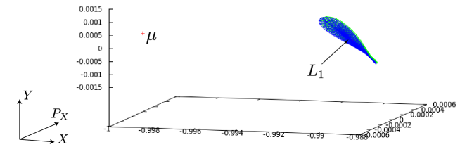
Fig. 5: A rough sketch of $\pi_{X,Y,P_{X}}\phi^{-1}(\bar{B}_{c}^{R-v}\times\bar{B}_{u}^{r}\times\bar{B}_{s}^{r})$, which gives us an idea of the actual size and thickness of the investigated region in which we have proved existence of the center manifold.

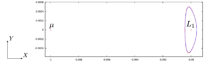
Fig. 6: A rough sketch of $\pi_{X,Y}\left(\phi^{-1}(\partial\bar{B}_{c}^{R-v}\times\bar{B}_{u}^{r}\times\bar{B}_{s}^{r})\right)$ in blue and $\pi_{X,Y}\left(\phi^{-1}(\partial\bar{B}_{c}^{R}\times\bar{B}_{u}^{r}\times\bar{B}_{s}^{r})\right)$ in red. We have proved that the manifold is contained in $\phi^{-1}(\bar{B}_{c}^{R-v}\times\bar{B}_{u}^{r}\times\bar{B}_{s}^{r})$ and that orbits starting from it never leave $\phi^{-1}(\bar{B}_{c}^{R}\times\bar{B}_{u}^{r}\times\bar{B}_{s}^{r})$ when going forwards or backwards in time.

6 Closing remarks, future work

In this paper we have given a method for detection and proof of existence of center manifolds in a practical domain of the system. We have successfully applied the method to the Restricted Three Body Problem. The method is quite general. It can be applied to any system with an integral of motion which allows for a computation of a normal form around a fixed point. The method also works for arbitrary dimension, which makes it a tool which can be applied to a large family of systems.

The strength of our approach lies in the fact that we can investigate and prove existence of manifolds within large domains, and not only locally around a fixed point. The weakness so far is that the method only establishes Lipschitz type continuity of the manifold. In forthcoming work we plan to remedy this deficiency. In our view, since we already have established Lipschitz continuity, similar tools combined with standard cohomology equation arguments can be applied to prove higher order smoothness.

We would also like to mention that the method allows for rigorous enclosure of the associated stable and unstable manifolds through cone conditions used in the proof. This means that the presented method can be used as a starting point for computation of foliations of stable/unstable manifolds, and next a scattering map associated with splitting of separatrices. In our future work we plan to conduct rigorous-computer-assisted computations of the scattering map for the RTBP in the spirit of [DMR]. Such computations can then be used in the study of structural stability or diffusion.

7 Acknowledgements

We would like to express our thanks to Daniel Wilczak for frequent discussions and his assistance in the implementation of higher order computations in the CAPD library (http://capd.ii.uj.edu.pl).

8 Appendix

Here we list the bounds needed for the verification of assumptions of Theorem 5. Below constants were computed using (93), (92) combined with (20), (10), (11) and (13)

$$\begin{array}[c]{lll}E_{u}=\mathtt{1.909815022732472,}&&E_{s}=\mathtt{1.909823931307315,}\\ \delta_{u}=\mathtt{2.434904529896616,}&&\delta_{s}=\mathtt{2.434911565550947,}\\ \varepsilon_{c}=\mathtt{0.09796031906285504,}&&\varepsilon_{m}=\mathtt{0.09656707906887786,}\\ \varepsilon_{u}=\mathtt{0.09737656524499766,}&&\varepsilon_{s}=\mathtt{0.09735689577043023.}\end{array}$$ (94)

Note that $[DF^{\phi}(D_{\phi})]$ and $[\pi_{x,y}F(\bar{B}_{c}^{R}\times\{0\}\times\{0\})]$ in (92), (93) are displayed with very rough accuracy. Above numbers follow from their precise version from the CAPD software.

From (9) we have obtained the bounds $c^{u},c^{s}$ (see (12)) using the following simple estimates. Our matrix $\mathbf{C}$ from (9) is of the form (see (92))

$$\mathbf{C}=\left(\begin{array}[c]{cc}\boldsymbol{\varepsilon}_{1}&\mathbf{r}_{1}\\ \mathbf{r}_{2}&\boldsymbol{\varepsilon}_{2}\end{array}\right).$$

For any matrix $C=\left(\begin{array}[c]{cc}\varepsilon_{1}&r_{1}\\ r_{2}&\varepsilon_{2}\end{array}\right)\in\mathbf{C}$ and any $\theta=\left(\theta_{1},\theta_{2}\right)$ for which $\left\|\theta\right\|=1,$ using

$$-\frac{1}{2}=-\frac{\theta_{1}^{2}+\theta_{2}^{2}}{2}\leq\theta_{1}\theta_{2}\leq\frac{\theta_{1}^{2}+\theta_{2}^{2}}{2}=\frac{1}{2}$$

we have

$$\theta^{T}C\theta$$

$$=\left(r_{1}+r_{2}\right)\theta_{2}\theta_{1}+\varepsilon_{1}\theta_{1}^{2}+\varepsilon_{2}\theta_{2}^{2}$$

$$\in\left[-\max_{r_{1}\in\mathbf{r}_{1},r_{2}\in\mathbf{r}_{2}}\frac{|r_{1}+r_{2}|}{2}+\min_{\varepsilon_{i}\in\boldsymbol{\varepsilon}_{i},i=1,2}\varepsilon_{i},\max_{r_{1}\in\mathbf{r}_{1},r_{2}\in\mathbf{r}_{2}}\frac{|r_{1}+r_{2}|}{2}+\max_{\varepsilon_{i}\in\boldsymbol{\varepsilon}_{i},i=1,2}\varepsilon_{i}\right].$$ (95)

The bound (95) is easily computable using interval arithmetic and (92)

$$\begin{array}[c]{lll}c^{u}=\mathtt{0.08050236551044671,}&&c^{s}=\mathtt{-0.08046115109310353.}\end{array}$$ (96)

Here once again the very rough rounding in (92) is evident when compared with (96).

Estimates (94), (96) give us

$$\begin{array}[c]{lll}\kappa_{c}^{\text{forw}}=\mathtt{\phantom{-}0.3233133031766185,}&&\kappa_{c}^{\text{back}}=\mathtt{-0.3232720887592754,}\\ \kappa_{u}^{\text{forw}}=\mathtt{\phantom{-}2.289103404031357,}&&\kappa_{u}^{\text{back}}=\mathtt{\phantom{-}2.191595652437820,}\\ \kappa_{s}^{\text{forw}}=\mathtt{-2.191592853354867,}&&\kappa_{s}^{\text{back}}=\mathtt{-2.289115357054329.}\end{array}$$ (97)

References

• [A] G. Alefeld, Inclusion methods for systems of nonlinear equations–the interval Newton method and modifications, Proceedings of the IMACS-GAMM International Workshop on Validated Computation, Topics in Validated Computations, Elsevier, Amsterdam, 1994, pp. 7-26.
• [B] Broucke, R. Periodic orbits in the restricted three–body problem with Earth–Moon masses NASA–JPL technical report 32-1168 (1968), available at http://ntrs.nasa.gov/archive/nasa/casi.ntrs.nasa.gov/19680013800_1968013800.pdf
• [CM] Canalias, E. and Masdemont, J. J. Homoclinic and heteroclinic transfer trajectories between planar Lyapunov orbits in the sun-earth and earth-moon systems Discrete Contin. Dyn. Syst. 14 no 2, 261-279 (2006)
• [CDMR] Canalias, E. and Delshams, A. and Masdemont, J. J. and Rold n, P. The scattering map in the planar restricted three body problem Celestial Mech. Dynam. Astronom. 95, 1-4, 155–171 (2006)
• [Ca] M. J. CapiΕ„ski, Covering Relations and the Existence of Topologically Normally Hyperbolic Invariant Sets, Discrete and Continuous Dynamical Systems A. Vol. 23, N. 3, (March 2009), pp 705-725.
• [CS] M. J. CapiΕ„ski, C. SimΓ³, Computer Assisted Proof for Normally Hyperbolic Maniflods, preprint.
• [CZ] M. J. CapiΕ„ski, P. ZgliczyΕ„ski, Cone Conditions and Covering Relations for Normally Hyperbolic Invariant Manifolds, preprint.
• [Car] J Carr, Applications of Centre Manifold Theory. Applied Mathematical Sciences N. 35, Springer-Verlag (1981).
• [CH] Chow, Shui Nee and Hale, Jack K. Methods of bifurcation theory Grundlehren der Mathematischen Wissenschaften [Fundamental Principles of Mathematical Science] New York (1982).
• [DMR] A. Delshams, J. Masdemont, P. RoldΓ‘n, Computing the scattering map in the spatial Hill’s problem. Discrete Contin. Dyn. Syst. Ser. B. Vol. 10, N. 2-3 (2008), pp 455–483.
• [GKLMMR] G mez, G. and Koon, W. S. and Lo, M. W. and Marsden, J. E. and Masdemont, J. and Ross, S. D. Connecting orbits and invariant manifolds in the spatial restricted three-body problem Nonlinearity 17, no 5, 1571–1606
• [GJSM] G mez, G. and Jorba, . and Sim , C. and Masdemont, J. Dynamics and mission design near libration points. Vol. III World Scientific Publishing Co. Inc. (2001)
• [GH] J. Guckenheimer, P. Holmes Nonlinear oscillations, dynamical systems, and bifurcations of vector fields. Springer-Verlag, New York, 1990.
• [Hi] M. Hirsh, Differential Topology, Graduate Texts in Mathematics, No. 33. Springer-Verlag, New York-Heidelberg, 1976
• [J] A. Jorba, A methodology for the numerical computation of normal forms, centre manifolds and first integrals of Hamiltonian systems. Experiment. Math. 8 (1999), no. 2, 155–195.
• [JS] Jorba, Angel and SimΓ³, Carles Effective stability for periodically perturbed Hamiltonian systems Hamiltonian mechanics (ToruΕ„, 1993) NATO Adv. Sci. Inst. Ser. B Phys. 331, 245–252 (1994)
• [JM] A. Jorba, J. Masdemont, Dynamics in the center manifold of the collinear points of the restricted three body problem. Phys. D. Vol. 132, N. 1-2 (1999), pp 189–213.
• [JV] Jorba, ngel and Villanueva, Jordi, Numerical computation of normal forms around some periodic orbits of the restricted three-body problem Phys. D, 114 no. 3-4, 197–229 (1998)
• [L] A. Lyapunov, ProblΓ¨me gΓ©nΓ©ral de la stabilitΓ© du mouvement, Ann. of Math. Studies, No. 17, Princeton Univ. Press, 1949.
• [MH] Meyer, Kenneth R. and Hall, Glen R. and Offin, Dan Introduction to Hamiltonian dynamical systems and the $N$-body problem Applied Mathematical Sciences, Springer, New York (2009)
• [M] J. Moser, On the Generalization of a theorem of A. Liapounoff, Communications on Pure and Applied Mathematics, Vol. xi (1958), 257-278.
• [Mu] J. Murdock, Normal forms and unfoldings for local dynamical systems. Springer Monographs in Mathematics (2003).
• [R] D. L. Richardson, A note on a Lagrangian formulation for motion about the collinear points. Celestial Mech. Vol. 22, N. 3 (1980), pp 231–236.
• [SM] C. L. Siegel, J. K. Moser, Lectures on celestial mechanics. Springer (1995).
• [Sij] J. Sijbrand, Properties of center manifolds. Trans. Amer. Math. Soc. Vol. 289, N. 2 (1985), pp 431–469.
• [S] V. Szebehely, Theory of Orbits, Academic Presss (1967).