Multiple testing via $\mbox{FDR}_{L}$ for large-scale imaging data

Abstract

The multiple testing procedure plays an important role in detecting the presence of spatial signals for large-scale imaging data. Typically, the spatial signals are sparse but clustered. This paper provides empirical evidence that for a range of commonly used control levels, the conventional $\operatorname{FDR}$ procedure can lack the ability to detect statistical significance, even if the $p$-values under the true null hypotheses are independent and uniformly distributed; more generally, ignoring the neighboring information of spatially structured data will tend to diminish the detection effectiveness of the $\operatorname{FDR}$ procedure. This paper first introduces a scalar quantity to characterize the extent to which the “lack of identification phenomenon” ($\operatorname{LIP}$) of the $\operatorname{FDR}$ procedure occurs. Second, we propose a new multiple comparison procedure, called $\operatorname{FDR}_{L}$, to accommodate the spatial information of neighboring $p$-values, via a local aggregation of $p$-values. Theoretical properties of the $\operatorname{FDR}_{L}$ procedure are investigated under weak dependence of $p$-values. It is shown that the $\operatorname{FDR}_{L}$ procedure alleviates the $\operatorname{LIP}$ of the $\operatorname{FDR}$ procedure, thus substantially facilitating the selection of more stringent control levels. Simulation evaluations indicate that the $\operatorname{FDR}_{L}$ procedure improves the detection sensitivity of the $\operatorname{FDR}$ procedure with little loss in detection specificity. The computational simplicity and detection effectiveness of the $\operatorname{FDR}_{L}$ procedure are illustrated through a real brain fMRI dataset.

, and

t1Supported by NSF Grant DMS-07-05209 and Wisconsin Alumni Research Foundation. t2Supported by NIH R01-GM072611 and NSF Grant DMS-07-14554.

1 Introduction

In many important applications, such as astrophysics, satellite measurement and brain imaging, the data are collected at spatial grid points, and a large-scale multiple testing procedure is needed for detecting the presence of spatial signals. For example, functional magnetic resonance imaging (fMRI) is a recent and exciting imaging technique that allows investigators to determine which areas of the brain are involved in a cognitive task. Since an fMRI dataset contains time-course measurements over voxels, the number of which is typically of the order of $10^{4}$–$10^{5}$, a multiple testing procedure plays an important role in detecting the regions of activation. Another example of important application of multiple testing is to the diffusion tensor imaging, which intends to identify brain white matter regions [Le Bihan et al. (2001)].

In the seminal work, Worsley et al. (2002) proposed a Gaussian random field method which approximates the family-wise error rate ($\operatorname{FWER}$) by modeling test statistics over the entire brain as a Gaussian random field. It has been found to be conservative in some cases [Nichols and Hayasaka (2003)]. Nichols and Hayasaka (2003) also discussed the use of permutation tests and their simulation studies showed that permutation tests tended to be more sensitive in finding activated regions. The false discovery rate ($\operatorname{FDR}$) approach has become increasingly popular. The conventional $\operatorname{FDR}$ procedure offers the advantage of overcoming the conservativeness drawback of $\operatorname{FWER}$, requiring fewer assumptions than random field based methods and being computationally less intensive than permutation tests.

Nevertheless, in practical applications to imaging data with a spatial structure, even if the $p$-values corresponding to the true null hypotheses are independent and uniformly distributed, the conventional $\operatorname{FDR}$ procedure may lack the ability to detect statistical significance, for a range of commonly used control levels $\alpha$. It will be seen, in the left panels of Figure 2, that the $\operatorname{FDR}$ procedure for a 2D simulated data declares only a couple of locations to be significant for $\alpha$ ranging from $0$ to about $0.4$. That is, even if we allow $\operatorname{FDR}$ to be controlled at the level $40\%$, one cannot reasonably well identify significant sites. The empirical evidence provided above for the standard $\operatorname{FDR}$ procedure is not pathological. Indeed, similar phenomena arise from commonly used signals plus noise models for imaging data, as will be exemplified by extensive studies in Section 4.2. In statistical literature, while some useful finite-sample and asymptotic results [Storey, Taylor and Siegmund (2004)] have been established for the $\operatorname{FDR}$ procedure, the results could not directly quantify the loss of power and “lack of identification phenomenon” ($\operatorname{LIP}$).

More generally, for spatially structured imaging data, the significant locations are typically sparse, but clustered rather than scattered. It is thus anticipated that a location and its adjacent neighbors fall in a similar type of region, either significant (active) or nonsignificant (inactive). As will be seen in the simulation studies (where the $\operatorname{LIP}$ does not occur) of Section 5, the existing $\operatorname{FDR}$ procedure tends to be less effective in detecting significance. This lack of detection efficiency is due to the information of $p$-values from adjacent neighbors not having been fully taken into account. Due to the popularity of the $\operatorname{FDR}$ procedure in research practices, it is highly desirable to embed the spatial information of imaging data into the $\operatorname{FDR}$ procedure.

This paper aims to quantify the $\operatorname{LIP}$ and to propose a new multiple testing procedure, called $\operatorname{FDR}_{L}$, for imaging data, to accommodate the spatial information of neighboring $p$-values, via a local aggregation of $p$-values. Main results are given in three parts.

• In the first part, statistical inference for the null distribution of locally aggregated $p$-values is studied. See Method I proposed in Section 3.2 and Method II in Section 3.3.

• In the second part, asymptotic properties of the $\operatorname{FDR}_{L}$ procedure are investigated under weak dependence (to be defined in Section 4.1) of $p$-values. See Theorems 4.1–4.3.

• The third part intends to provide a more in-depth discussion of why the $\operatorname{LIP}$ occurs and the extent to which the $\operatorname{FDR}_{L}$ procedure alleviates the $\operatorname{LIP}$. In particular, we introduce a scalar $\alpha_{\infty}$ to quantify the $\operatorname{LIP}$: the smaller the $\alpha_{\infty}$, the smaller control level can be adopted without encountering $\operatorname{LIP}$; $\alpha_{\infty}=0$ rules out the possibility of the $\operatorname{LIP}$. In the particular case of i.i.d. $p$-values, Theorem 4.4 provides verifiable conditions under which $\alpha_{\infty}=0$ and under which $\alpha_{\infty}>0$. Theorem 4.5 demonstrates that under mild conditions, $\alpha_{\infty}$ of the $\operatorname{FDR}_{L}$ procedure is lower than the counterpart of the $\operatorname{FDR}$ procedure. These theoretical results demonstrate that the $\operatorname{FDR}_{L}$ procedure alleviates the extent of the $\operatorname{LIP}$, thus substantially facilitates the selection of user-specified control levels. As observed from the middle and right panels of Figure 2, for control levels close to zero, the $\operatorname{FDR}_{L}$ procedure combined with either Method I or Method II identifies a larger number of true significant locations than the $\operatorname{FDR}$ procedure.

The rest of the paper is arranged as follows. Section 2 reviews the conventional $\operatorname{FDR}$ procedure and introduces $\alpha_{\infty}$ to characterize the $\operatorname{LIP}$. Section 3 describes the proposed $\operatorname{FDR}_{L}$ procedure. Its theoretical properties are established in Section 4, where Section 4.2 explores the extent to which the $\operatorname{FDR}_{L}$ procedure alleviates $\operatorname{LIP}$. Sections 5 and 6 present simulation comparisons of the $\operatorname{FDR}$ and $\operatorname{FDR}_{L}$ procedures in 2D and 3D dependent data, respectively. Section 7 illustrates the computational simplicity and detection effectiveness of the proposed method for a real brain fMRI dataset for detecting the regions of activation. Section 8 ends the paper with a brief discussion. Technical conditions and detailed proofs are deferred to the Appendix.

2 $\operatorname{FDR}$ and lack of identification phenomenon

2.1 Conventional $\operatorname{FDR}$ procedure

We begin with a brief overview of the conventional $\operatorname{FDR}$ procedure that is of particular relevance to the discussion in Sections 3 and 4. For testing a family of null hypotheses, $\{H_{0}(i)\}_{i=1}^{n}$, suppose that $p_{i}$ is the $p$-value of the $i$th test. Table 1 summarizes the outcomes.

=280pt $\bolds{H_{0}(i)}$ retained $\bolds{H_{0}(i)}$ rejected Total $H_{0}(i)$ true $U$ $V$ $n_{0}$ $H_{0}(i)$ false $T$ $S$ $n_{1}$ Total $W$ $R$ $n$

Table 1: Outcomes from testing $n$ (null) hypotheses $H_{0}(i)$ based on a significance rule

Benjamini and Hochberg (1995) proposed a procedure that guarantees the False Discovery Rate ($\operatorname{FDR}$) to be less than or equal to a pre-selected value. Here, the $\operatorname{FDR}$ is the expected ratio of the number of incorrectly rejected hypotheses to the total number of rejected hypotheses with the ratio defined to be zero if no hypothesis is rejected, that is, $\operatorname{FDR}=E(\frac{V}{R\vee 1})$ where $R\vee 1=\max(R,1)$. A comprehensive overview of the development of the research in the area of multiple testing can be found in Benjamini and Yekutieli (2001), Genovese and Wasserman (2002), Storey (2002), Dudoit, Shaffer and Boldrick (2003), Efron (2004), Storey, Taylor and Siegmund (2004), Genovese and Wasserman (2004), Lehmann and Romano (2005), Lehmann, Romano and Shaffer (2005), Genovese, Roeder and Wasserman (2006), Sarkar (2006), Benjamini and Heller (2007) and Wu (2008), among others. Fan, Hall and Yao (2007) addressed the issue on the number of hypotheses that can be simultaneously tested when the $p$-values are computed based on asymptotic approximations.

Storey, Taylor and Siegmund (2004) gave an empirical process definition of $\operatorname{FDR}$, by

$$\operatorname{FDR}(t)=E\biggl{\{}\frac{V(t)}{R(t)\vee 1}\biggr{\}},$$ (1)

where $t$ stands for a threshold for $p$-values. For realistic applications, Storey (2002) proposed the point estimate of $\operatorname{FDR}(t)$ by

$$\widehat{\operatorname}{FDR}(t)=\frac{W(\lambda)t}{\{R(t)\vee 1\}(1-\lambda)},$$ (2)

where $\lambda\in(0,1)$ is a tuning constant, and $W(t)$ is the number of nonrejections with a threshold $t$. The intuition of this will be explained in Section 3.4. The pointwise limit of $\widehat{\operatorname}{FDR}(t)$ under assumptions (7)–(9) of Storey, Taylor and Siegmund (2004) is

$$\widehat{\operatorname{FDR}}^{\infty}(t)=\frac{[\pi_{0}\{1-G_{0}(\lambda)\}+\pi_{1}\{1-G_{1}(\lambda)\}]t}{\{\pi_{0}G_{0}(t)+\pi_{1}G_{1}(t)\}(1-\lambda)},$$ (3)

where $\pi_{0}=\lim_{n\to\infty}n_{0}/n$, $\pi_{1}=1-\pi_{0}$, and $\lim_{n\to\infty}V(t)/n_{0}=G_{0}(t)$ and $\lim_{n\to\infty}S(t)/n_{1}=G_{1}(t)$ are assumed to exist almost surely for each $t\in(0,1]$. For a pre-chosen level $\alpha$, a data-driven threshold for $p$-values is determined by

$$t_{\alpha}(\widehat{\operatorname}{FDR})=\sup\{0\leq t\leq 1\dvtx\widehat{\operatorname}{FDR}(t)\leq\alpha\}.$$ (4)

A null hypothesis is rejected if the corresponding $p$-value is less than or equal to the threshold $t_{\alpha}(\widehat{\operatorname}{FDR})$. Methods (2) and (4) form the basis for the conventional $\operatorname{FDR}$ procedure.

2.2 Proposed measure for lack of identification phenomenon

Recall that the $\operatorname{FDR}$ procedure is essentially a threshold-based approach for multiple testing problems, where the data-driven threshold $t_{\alpha}(\widehat{\operatorname}{FDR})$ plays a key role. It is clearly seen from (4) that $t_{\alpha}(\widehat{\operatorname}{FDR})$ hinges on both the estimates $\widehat{\operatorname}{FDR}(t)$ devised, as well as the control level $\alpha$ specified.

Using (2), we observe that the corresponding $t_{\alpha}(\widehat{\operatorname}{FDR})$ is a nondecreasing function of $\alpha$. This indicates that for the $\operatorname{FDR}$ procedure, as $\alpha$ decreases below $\inf_{0<t\leq 1}\widehat{\operatorname}{FDR}(t)$, the threshold $t_{\alpha}(\widehat{\operatorname}{FDR})$ will drop to zero and accordingly, the $\operatorname{FDR}$ procedure can only reject those hypotheses with $p$-values exactly equal to zero. We call this phenomenon “lack of identification.”

To better quantify the “lack of identification phenomenon” ($\operatorname{LIP}$), the limiting forms of $\widehat{\operatorname}{FDR}(t)$ as $n\to\infty$ will be examined.

Definition 1.

For estimation methods $\widehat{\operatorname}{FDR}(t)$ in (2), define

$$\alpha_{\infty}^{\operatorname{FDR}}=\inf_{0<t\leq 1}\widehat{\operatorname}{FDR}^{\infty}(t),$$

where $\widehat{\operatorname}{FDR}^{\infty}(t)$ is defined in (3). Define the endurance by $E_{\operatorname{FDR}}=1-\alpha_{\infty}^{\operatorname{FDR}}$.

Notice that the existence of $\alpha_{\infty}^{\operatorname{FDR}}>0$ implies the occurrence of the $\operatorname{LIP}$: in real data applications with a moderately large number $n$ of hypotheses, the $\operatorname{FDR}$ procedure loses the identification capability when the control level $\alpha$ is close to or smaller than $\alpha_{\infty}^{\operatorname{FDR}}$. On the other hand, the case $\alpha_{\infty}^{\operatorname{FDR}}=0$ rules out the possibility of the $\operatorname{LIP}$. Henceforth, the smaller the $\alpha_{\infty}^{\operatorname{FDR}}$, the higher endurance of the corresponding $\widehat{\operatorname}{FDR}$, and the less likely the $\operatorname{LIP}$ happens. In other words, an $\operatorname{FDR}$ estimation approach with a higher endurance is more capable of adopting a smaller control level, thus reducing the extent of the $\operatorname{LIP}$ problem. We will revisit this issue in Section 4.2 after introducing the proposed $\operatorname{FDR}_{L}$ procedure.

3 Proposed $\operatorname{FDR}_{L}$ procedure for imaging data

Consider a set of spatial signals $\{\mu(v)\dvtx v\in\mathcal{V}\subseteq\mathbb{Z}^{d}\}$ in a 2D plane ($d=2$) or a 3D space ($d=3$), where $\mu(v)=0$ for $v\in\mathcal{V}_{0}$, $\mu(v)\neq 0$ for $v\in\mathcal{V}_{1}$ and $\mathcal{V}_{0}\cup\mathcal{V}_{1}=\mathcal{V}$. Here $\mathcal{V}_{0}$ and $\mathcal{V}_{1}$ are unknown sets. A common approach for detecting the presence of the spatial signals consists of two stages. In the first stage, test the hypothesis

$$H_{0}(v)\dvtx\mu(v)=0\quad{\mbox{versus}}\quad H_{1}(v)\dvtx\mu(v)\neq 0$$

at each location $v$. The corresponding $p$-value is denoted by $p(v)$. In the second stage, a multiple testing procedure, such as the conventional $\operatorname{FDR}$ procedure, is applied to the collection, $\{p(v)\dvtx v\in\mathcal{V}\subseteq\mathbb{Z}^{d}\}$, of $p$-values.

In the second stage, instead of using the original $p$-value, $p(v)$, at each $v$, we propose to use a local aggregation of $p$-values at points located adjacent to $v$. We summarize the procedure as follows.

Step 1.

Choose a local neighborhood with size $k$.

Step 2.

At each grid point $v$, find the set $N_{v}$ of its neighborhood points, and the set $\{p(v^{\prime})\dvtx v^{\prime}\in N_{v}\}$ of the corresponding $p$-values.

Step 3.

At each grid point $v$, apply a transformation $f\dvtx[0,1]^{k}\mapsto[0,1]$ to the set of $p$-values in Step 2, leading to a “locally aggregated” quantity, $p^{*}(v)=f(\{p(v^{\prime})\dvtx v^{\prime}\in N_{v}\})$.

Step 4.

Determine a data-driven threshold for $\{p^{*}(v)\dvtx v\in\mathcal{V}\subseteq\mathbb{Z}^{d}\}$.

For notational clarity, we denote by $\{p_{i}^{*}\}_{i=1}^{n}$ the collection of “locally aggregated” $p^{*}$-values, $\{p^{*}(v)\dvtx v\in\mathcal{V}\subseteq\mathbb{Z}^{d}\}$. Likewise, the notation $U^{*}(t)$, $V^{*}(t)$, $T^{*}(t)$, $S^{*}(t)$, $W^{*}(t)$ and $R^{*}(t)$ can be defined as in Section 2, with $p_{i}$ replaced by $p_{i}^{*}$. For instance, $V^{*}(t)=\sum_{i=1}^{n}\mathrm{I}\{H_{0}(i)$ is true, and $p_{i}^{*}\leq t\}$ and $R^{*}(t)=\sum_{i=1}^{n}\mathrm{I}(p_{i}^{*}\leq t)$, with $\mathrm{I}(\cdot)$ an indicator function. Accordingly, the false discovery rate based on utilizing the locally aggregated $p_{i}^{*}$-values becomes

$$\operatorname{FDR}_{L}(t)=E\biggl{\{}\frac{V^{*}(t)}{R^{*}(t)\vee 1}\biggr{\}}.$$ (5)

As a comparison, $\operatorname{FDR}(t)$ in (1) corresponds to the use of the original $p$-values.

3.1 Choice of neighborhood and choice of $f$

As in Roweis and Saul (2000), the set of neighbors for each data point can be assigned in a variety of ways, by choosing the $k$ nearest neighbors in Euclidean distance, by considering all data points within a ball of fixed radius or by using some prior knowledge.

For the choice of the transformation function, $f$, one candidate is the median filter, applied to the neighborhood $p$-values, without having to specify particular forms of spatial structure. A discussion on other options for $f$ can be found in Section 8. Unless otherwise stated, this paper focuses on the median filtering.

3.2 Statistical inference for $p^{*}$-values: Method $\mathrm{I}$

Let $G^{*}(\cdot)$ be the cumulative distribution function of a “locally aggregated” $p^{*}$-value corresponding to the true null hypothesis. Let $\widetilde{G}^{*}(\cdot)$ be the sample distribution of $\{p^{*}(v):v\in\mathcal{V}_{0}\}$. Recall that the original $p$-value corresponding to the true null hypothesis is uniformly distributed on the interval $(0,1)$. In contrast, the distribution $G^{*}(\cdot)$ for a “locally aggregated” $p^{*}$-value is typically nonuniform. This indicates that a significance rule based on $p$-values is not directly applicable to the significance rule based on $p^{*}$-values. For the median operation $f$, we propose two methods for estimating $\widetilde{G}^{*}(\cdot)$. Method I is particularly useful for large-scale imaging datasets, whereas Method II is useful for data of limited resolution.

Method I is motivated from the observation: if the original $p$-values are independent and uniformly distributed on the interval $(0,1)$, then the median aggregated $p^{*}$-value follows a Beta distribution. More precisely, if the neighborhood size $k$ is an odd integer, then the median aggregated $p^{*}$-value conforms to the

$$\operatorname{Beta}\bigl{(}(k+1)/2,(k+1)/2\bigr{)}$$ (6)

distribution [Casella and Berger (1990)]. If $k$ is an even integer, the median aggregated $p^{*}$-value is distributed as a random variable $(X+Y)/{2}$, where $(X,Y)$ has the joint probability density function ${k!}/{\{(k/2-1)!\}^{2}}x^{k/2-1}(1-y)^{k/2-1}\mathrm{I}(0<x<y<1)$. Thus, as long as the resolution of the experiment data and imaging technique keeps improving, so that the proportion of boundary grid points (corresponding to those with neighborhood intersected with both $\mathcal{V}_{0}$ and $\mathcal{V}_{1}$) decreases and eventually shrinks to zero, $G^{*}(\cdot)$ will tend to the Beta distribution in (6).

Following this argument, if the original $p$-values corresponding to the true null hypotheses are independent and uniformly distributed [see, e.g., van der Vaart (1998), page 305], the median aggregated $p^{*}$-values corresponding to the true null hypotheses will approximately be symmetrically distributed about $0.5$. Thus, assuming that the number of false null hypothesis with $p_{i}^{*}>0.5$ is negligible, the total number of true null hypotheses, $n_{0}$, is approximately $2\sum_{i=1}^{n}\mathrm{I}(p_{i}^{*}>0.5)+\sum_{i=1}^{n}\mathrm{I}(p_{i}^{*}=0.5)$, and the number of true null hypotheses with $p^{*}$-values smaller than or equal to $t$ could be estimated by $\sum_{i=1}^{n}\mathrm{I}\{p_{i}^{*}\geq(1-t)\}$, for small values of $t$. Here, owing to the symmetry, we use the upper tail to compute the proportion to mitigate the bias caused by the data from the alternative hypotheses. Hence, $\widetilde{G}^{*}(t)$ can be estimated by the empirical distribution function,

$$\widehat{G}^{*}(t)=\cases{\dfrac{\sum_{i=1}^{n}\mathrm{I}\{p_{i}^{*}\geq(1-t)\}}{2\sum_{i=1}^{n}\mathrm{I}(p_{i}^{*}>0.5)+\sum_{i=1}^{n}\mathrm{I}(p_{i}^{*}=0.5)},\vspace*{3pt}\cr\qquad\mbox{if $0\leq t\leq 0.5$},\vspace*{3pt}\cr 1-\dfrac{\sum_{i=1}^{n}\mathrm{I}(p_{i}^{*}>t)}{2\sum_{i=1}^{n}\mathrm{I}(p_{i}^{*}>0.5)+\sum_{i=1}^{n}\mathrm{I}(p_{i}^{*}=0.5)},\vspace*{3pt}\cr\qquad\mbox{if $0.5<t\leq 1$}.}$$ (7)

A modification of the Glivenko–Cantelli theorem shows that ${\sup_{0\leq t\leq 1}}|\widehat{G}^{*}(t)-G^{*}(t)|=o(1)$ almost surely as $n\to\infty$. This method is distribution free, computationally fast and applicable when the $p^{*}$-values under the null hypotheses are not too skewedly distributed.

An alternative approach for approximating $\widetilde{G}^{*}(\cdot)$ is inspired by the central limit theorem. If the neighborhood size $k$ is reasonably large (e.g., $k\geq 5$ if the original $p$-values corresponding to the true null hypotheses are independent and uniformly distributed), then $\widetilde{G}^{*}(\cdot)$ could be approximated by a normal distribution centered at $0.5$. This normal approximation scheme may be exploited in the situation (which rarely occurs, though) when the original $p$-values corresponding to the true null hypotheses are independent but asymmetric about $0.5$ (when the null distribution function of the test statistic is discontinuous).

3.3 Refined method for estimating $\widetilde{G}^{*}(\cdot)$: Method $\mathrm{II}$

More generally, we consider spatial image data of limited resolution. Recall the neighborhood size $k$ of a voxel $v$ in the paper includes one for $v$ itself. Let $\mathsf{n}_{1}(v)$ denote the number of points in $N_{v}$ that belong to $\mathcal{V}_{1}$. Thus for any grid point $v\in\mathcal{V}_{0}$, $\mathsf{n}_{1}(v)$ takes values $\{0,1,\ldots,k-1\}$. Set

$$\theta_{n,j}=P\{\mathsf{n}_{1}(v)=j\},\qquad Q_{j}^{*}(t)=P\{p^{*}(v)\leq t|\mathsf{n}_{1}(v)=j\}.$$

Clearly, $\sum_{j=0}^{k-1}\theta_{n,j}=1$. Therefore, the C.D.F. of $p^{*}(v)$ for a grid point $v\in\mathcal{V}_{0}$ is given by

$$G^{*}(t)=\theta_{n,0}Q_{0}^{*}(t)+\theta_{n,1}Q_{1}^{*}(t)+\cdots+\theta_{n,k-1}Q_{k-1}^{*}(t),$$ (8)

where $Q_{0}^{*}(t)$ corresponds to, for independent tests, the Beta distribution function in (6).

Likewise, we obtain

$$\widetilde{G}^{*}(t)=\sum_{j=0}^{k-1}\widetilde{\theta}_{n,j}\widetilde{Q}_{j}^{*}(t),$$

where $\widetilde{\theta}_{n,j}={\#\mathcal{V}_{0}^{(j)}}/{n_{0}}$ is the proportion of $v\in\mathcal{V}_{0}$ with $j$ neighboring grid points in $\mathcal{V}_{1}$, and $\widetilde{Q}_{j}^{*}(t)={\sum_{v\in\mathcal{V}_{0}^{(j)}}\mathrm{I}\{p^{*}(v)\leq t\}}/{\#\mathcal{V}_{0}^{(j)}}$ is the sample distribution of $\{p^{*}(v):v\in\mathcal{V}_{0}^{(j)}\}$, with $\#A$ denoting the number of elements in a set $A$ and $\mathcal{V}_{0}^{(j)}=\{v\in\mathcal{V}_{0}\dvtx\mathsf{n}_{1}(v)=j\}$. Clearly, if the original $p$-values corresponding to the true null hypotheses are block dependent, then, by the Glivenko–Cantelli theorem, $\sup_{0\leq t\leq 1}|\widetilde{G}^{*}(t)-G^{*}(t)|=o(1)$ almost surely, as $n\to\infty$.

We propose the following Method II to estimate $\widetilde{G}^{*}(t)$:

1. Obtain estimates $\widehat{n}_{0}$ and $\widehat{n}_{1}=n-\widehat{n}_{0}$ of $n_{0}$ and $n_{1}$, respectively. One possible estimator of $n_{0}$ is $\widehat{n}_{0}={\sum_{i=1}^{n}\mathrm{I}(p_{i}^{*}>\lambda)}/\{1-\widehat{G}^{*}(\lambda)\}$, for some tuning parameter $\lambda$.

2. Define $\widehat{\mathcal{V}}_{1}=\{v\in\mathcal{V}\dvtx p^{*}(v)\leq p_{(\widehat{n}_{1})}^{*}\}$, where $\{p_{(i)}^{*}\}_{i=1}^{n}$ denote the order statistics of $\{p_{i}^{*}\}_{i=1}^{n}$. Define $\widehat{\mathcal{V}}_{0}=\{v\in\mathcal{V}\dvtx p^{*}(v)>p_{(\widehat{n}_{1})}^{*}\}$.

3. Set $\widehat{\mathcal{V}}_{0}^{(j)}=\{v\in\widehat{\mathcal{V}}_{0}\dvtx\mathsf{n}_{1}(v)=j\}$. Estimate $\widetilde{\theta}_{n,j}$, $j=0,\ldots,k-1$, by $\widehat{\theta}_{n,j}={\#\widehat{\mathcal{V}}_{0}^{(j)}}/{\widehat{n}_{0}}$.

4. For $j=0$, estimate $\widetilde{Q}_{0}^{*}(t)$ by $\widehat{Q}_{0}^{*}(t)=\widehat{G}^{*}(t)$, the estimator of $\widetilde{G}^{*}(t)$ by Method I in Section 3.2. To estimate $\widetilde{Q}_{j}^{*}(t)$, $j=1,\ldots,k-1$, for each $v\in\widehat{\mathcal{V}}_{0}^{(0)}$, collect its neighborhood $p$-values, randomly exclude $j$ of them and obtain the set $D_{j}(v)$ for the remaining neighborhood $p$-values. Randomly sample $j$ grid points from $\widehat{\mathcal{V}}_{1}$ and collect their corresponding $p$-values in a set $A_{j}(v)$. Compute the median, $\widehat{p}_{j}^{*}(v)$, of $p$-values in $D_{j}(v)\cup A_{j}(v)$. Estimate $\widetilde{Q}_{j}^{*}(t)$ by $\widehat{Q}_{j}^{*}(t)={\sum_{v\in\widehat{\mathcal{V}}_{0}^{(0)}}\mathrm{I}\{\widehat{p}_{j}^{*}(v)\leq t\}}/{\#\widehat{\mathcal{V}}_{0}^{(0)}}$.

5. Combining (8), $\widetilde{G}^{*}(t)$ is estimated by $\widehat{G}_{c}^{*}(t)=\sum_{j=0}^{k-1}\widehat{\theta}_{n,j}\widehat{Q}_{j}^{*}(t)$.

3.4 Significance rule for $p^{*}$-values

Using the locally aggregated $p^{*}$-values, we can estimate $\operatorname{FDR}_{L}(t)$ defined in (5) by either

$$\widehat{\operatorname}{FDR}_{L}(t)=\frac{W^{*}(\lambda)\widehat{G}^{*}(t)}{\{R^{*}(t)\vee 1\}\{1-\widehat{G}^{*}(\lambda)\}},$$ (9)

using Method I, or

$$\widehat{\operatorname}{FDR}_{L}(t)=\frac{W^{*}(\lambda)\widehat{G}_{c}^{*}(t)}{\{R^{*}(t)\vee 1\}\{1-\widehat{G}_{c}^{*}(\lambda)\}},$$ (10)

using Method II. The logic behind this estimate is the following. If we choose $\lambda$ far enough from zero, then the number of nonrejections, $W^{*}(\lambda)$, is roughly $U^{*}(\lambda)$. Using this, we have

$$V^{*}(\lambda)\approx n_{0}\widetilde{G}^{*}(\lambda)\approx\{V^{*}(\lambda)+W^{*}(\lambda)\}\widetilde{G}^{*}(\lambda).$$

Solving the above equation suggests an estimate of $V^{*}(\lambda)$ by ${W^{*}(\lambda)\widetilde{G}^{*}(\lambda)}/\{1-\widetilde{G}^{*}(\lambda)\}$. Now, using $V^{*}(t)/V^{*}(\lambda)\approx\widetilde{G}^{*}(t)/\widetilde{G}^{*}(\lambda)$, we obtain that at a threshold $t$, $V^{*}(t)$ can be estimated by ${W^{*}(\lambda)\widetilde{G}^{*}(t)}/\{1-\widetilde{G}^{*}(\lambda)\}$. This together with the definition of $\operatorname{FDR}_{L}(t)$ in (5) suggests the estimate in (9). Interestingly, in the particular case of $p_{i}^{*}\equiv p_{i}$ and $\widehat{G}^{*}(t)=t$ [or $\widehat{G}_{c}^{*}(t)=t$], $\widehat{\operatorname}{FDR}_{L}(t)$ coincides with $\widehat{\operatorname}{FDR}(t)$ defined in (2).

For a given control level $\alpha$, a null hypothesis is rejected if the associated $p^{*}$-value is smaller than or equal to the threshold,

$$t_{\alpha}(\widehat{\operatorname}{FDR}_{L})\equiv\sup\{0\leq t\leq 1\dvtx\widehat{\operatorname}{FDR}_{L}(t)\leq\alpha\}.$$ (11)

This data-driven threshold for $p^{*}$-values together with the point estimation method (9) [or (10)] for the false discovery rates comprises the proposed $\operatorname{FDR}_{L}$ procedure.

4 Properties of the $\operatorname{FDR}_{L}$ procedure

4.1 Asymptotic behavior

This section explores the asymptotic behavior of the $\operatorname{FDR}_{L}$ procedure under weak dependence of $p$-values. Technical assumptions are given in Condition A in the Appendix, where Conditions A1–A3 are similar to assumptions $(7)$–$(9)$ of Storey, Taylor and Siegmund (2004). Thus the type of dependence in Condition A2 includes finite block dependence, and certain mixing dependence. Theorems 4.1–4.3 can be considered a generalization of Storey, Taylor and Siegmund (2004) from a single $p$-value to locally aggregating a number $k$ of $p$-values with $k>1$.

Theorem 4.1 below reveals that the proposed estimator $\widehat{\operatorname}{FDR}_{L}(t)$ controls the $\operatorname{FDR}_{L}(t)$ simultaneously for all $t\geq\delta$ with $\delta>0$, and in turn supplies a conservative estimate of $\operatorname{FDR}_{L}(t)$.

Theorem 4.1

Assume Condition A in Appendix A. For each $\delta>0$,

$$\lim_{n\to\infty}\inf_{t\geq\delta}\biggl{\{}\widehat{\operatorname}{FDR}_{L}(t)-\frac{V^{*}(t)}{R^{*}(t)\vee 1}\biggr{\}}\geq 0$$

and

$$\lim_{n\to\infty}\inf_{t\geq\delta}\{\widehat{\operatorname}{FDR}_{L}(t)-\operatorname{FDR}_{L}(t)\}\geq 0$$

with probability one.

To show that the proposed $\widehat{\operatorname}{FDR}_{L}(t)$ asymptotically provides a strong control of $\operatorname{FDR}_{L}(t)$, we define

$$\widehat{\operatorname}{FDR}_{L}^{\infty}(t)=\frac{[\pi_{0}\{1-G_{0}^{*}(\lambda)\}+\pi_{1}\{1-G_{1}^{*}(\lambda)\}]G^{*\infty}(t)}{\{\pi_{0}G_{0}^{*}(t)+\pi_{1}G_{1}^{*}(t)\}\{1-G^{*\infty}(\lambda)\}},$$ (12)

which is the pointwise limit of $\widehat{\operatorname}{FDR}_{L}(t)$ under Condition A in Appendix A, where it is assumed that $\pi_{0}=\lim_{n\to\infty}n_{0}/n$, and $\lim_{n\to\infty}{V^{*}(t)}/{n_{0}}=G_{0}^{*}(t)$ and $\lim_{n\to\infty}{S^{*}(t)}/{n_{1}}=G_{1}^{*}(t)$ exist almost surely for each $t\in(0,1]$, and $G^{*\infty}(t)=\lim_{n\to\infty}G^{*}(t)$.

Theorem 4.2

Assume Condition A in Appendix A. If there is a $t\in(0,1]$ such that $\widehat{\operatorname}{FDR}_{L}^{\infty}(t)<\alpha$, then $\limsup_{n\to\infty}\operatorname{FDR}_{L}(t_{\alpha}(\widehat{\operatorname}{FDR}_{L}))\leq\alpha$.

Theorem 4.3 states that the random thresholding rule $t_{\alpha}(\widehat{\operatorname}{FDR}_{L})$ converges to the deterministic rule $t_{\alpha}(\widehat{\operatorname}{FDR}_{L}^{\infty})$.

Theorem 4.3

Assume Condition A in Appendix A. If $\widehat{\operatorname}{FDR}_{L}^{\infty}(\cdot)$ has a nonzero derivative at the point $t_{\alpha}(\widehat{\operatorname}{FDR}_{L}^{\infty})\in(0,1)$, then $\lim_{n\to\infty}t_{\alpha}(\widehat{\operatorname}{FDR}_{L})=t_{\alpha}(\widehat{\operatorname}{FDR}_{L}^{\infty})$ holds almost surely.

4.2 Conditions for lack of identification phenomenon

Definition 2.

For estimation methods $\widehat{\operatorname}{FDR}_{L}(t)$ in (9) [or (10)], define

$$\alpha_{\infty}^{\operatorname{FDR}_{L}}=\inf_{0<t\leq 1}\widehat{\operatorname}{FDR}_{L}^{\infty}(t),$$

where $\widehat{\operatorname}{FDR}_{L}^{\infty}(t)$ is defined in (12).

Theorem 4.4 establishes conditions under which the $\operatorname{LIP}$ does or does not take place with the $\operatorname{FDR}$ and $\operatorname{FDR}_{L}$ procedures. It will be seen that the conditions are characterized by the null and alternative distributions of the test statistics, without relying on the configuration of the neighborhood used in the $\operatorname{FDR}_{L}$ procedure. Theorem 4.5 demonstrates that $\alpha_{\infty}^{\operatorname{FDR}}\geq\alpha_{\infty}^{\operatorname{FDR}_{L}}$ under mild conditions, thus the $\operatorname{FDR}_{L}$ procedure reduces the extent of the $\operatorname{LIP}$. For expository brevity, we assume the test statistics are independent, which can be relaxed.

Theorem 4.4

Let $\{T(v)\dvtx v\in\mathcal{V}\subseteq\mathbb{Z}^{d}\}$ be the set of test statistics for testing the presence of the spatial signals $\{\mu(v)\dvtx v\in\mathcal{V}\subseteq\mathbb{Z}^{d}\}$. Consider the one-sided testing problem,

$$H_{0}(v)\dvtx\mu(v)=0\quad{\mbox{versus}}\quad H_{1}(v)\dvtx\mu(v)>0.$$ (13)

For $j=0$ and $j=1$, respectively, assume that $T(v)$, corresponding to the true $H_{j}(v)$, are i.i.d. random variables having a cumulative distribution function $F_{j}$ with a probability density function $f_{j}$. Assume that the neighborhood size $k\geq 3$ used in the $\operatorname{FDR}_{L}$ procedure is an odd integer and that the proportion of boundary grid points within $\mathcal{V}_{0}$ shrinks to zero, as $n\to\infty$, that is, $\lim_{n\to\infty}{\#\mathcal{V}_{0}^{(0)}}/{n_{0}}=1$, where $\mathcal{V}_{0}^{(0)}=\{v\in\mathcal{V}\dvtx\mu(v^{\prime})=0$ for any $v^{\prime}\in N_{v}\}.$ Assume Condition A1 in Appendix A. Let $x_{0}=F_{0}^{-1}(1)=\inf\{t\dvtx F_{0}(t)=1\}$. [$\mathrm{II}.$]

If $\lim_{x\to x_{0}-}\frac{f_{1}(x)}{f_{0}(x)}=\infty,$ then $\alpha_{\infty}^{\operatorname{FDR}}=0$ and $\alpha_{\infty}^{\operatorname{FDR}_{L}}=0$.

If $\limsup_{x\to x_{0}-}\frac{f_{1}(x)}{f_{0}(x)}<\infty,$ then $\alpha_{\infty}^{\operatorname{FDR}}>0$ and $\alpha_{\infty}^{\operatorname{FDR}_{L}}>0$.

Theorem 4.5

Assume the conditions in Theorem 4.4. Suppose that $f_{0}(\cdot)$ is supported in an interval; $f_{1}(x)\leq f_{0}(x)$ for any $x\leq F_{0}^{-1}(0.5)$; $1-F_{0}(F_{1}^{-1}(0.5))\leq\lambda\leq 0.5$. Then $\alpha_{\infty}^{\operatorname{FDR}}\geq\alpha_{\infty}^{\operatorname{FDR}_{L}}$.

Corollaries 1 and 2 below provide concrete applications of Theorems 4.4 and 4.5. The detailed verifications are omitted.

Corollary 1.

Assume the conditions in Theorem 4.4. Suppose that the distribution $F_{0}$ is $N(0,1)$ and the distribution $F_{1}$ is $N(C,\sigma^{2})$, where $\sigma\in(0,\infty)$ and $C\in(0,\infty)$ are constants. [$\mathrm{II}.$]

If $\sigma\geq 1$, then $\alpha_{\infty}^{\operatorname{FDR}}=0$ and $\alpha_{\infty}^{\operatorname{FDR}_{L}}=0$.

If $0<\sigma<1$, then $\alpha_{\infty}^{\operatorname{FDR}}>0$ and $\alpha_{\infty}^{\operatorname{FDR}_{L}}>0$. Moreover, if $\exp\{-(C/\sigma)^{2}/2\}/\break{\sigma}\leq 1$ and $1-F_{0}(C)\leq\lambda\leq 0.5$, then $\alpha_{\infty}^{\operatorname{FDR}}\geq\alpha_{\infty}^{\operatorname{FDR}_{L}}$.

Corollary 2.

Assume the conditions in Theorem 4.4. Suppose that the distribution $F_{0}$ is that of a Student’s $t_{d_{0}}$ variate with $d_{0}$ degrees of freedom and the distribution $F_{1}$ is that of $C$ plus a Student’s $t_{d_{1}}$ variate with $d_{1}$ degrees of freedom, where $C\in(0,\infty)$ is a constant. [$\mathrm{II}.$]

If $d_{0}>d_{1}$, then $\alpha_{\infty}^{\operatorname{FDR}}=0$ and $\alpha_{\infty}^{\operatorname{FDR}_{L}}=0$.

If $1\leq d_{0}\leq d_{1}$, then $\alpha_{\infty}^{\operatorname{FDR}}>0$ and $\alpha_{\infty}^{\operatorname{FDR}_{L}}>0$. Moreover, if $d_{0}=d_{1}$ and $1-F_{0}(C)\leq\lambda\leq 0.5$, then $\alpha_{\infty}^{\operatorname{FDR}}\geq\alpha_{\infty}^{\operatorname{FDR}_{L}}$.

Remark 1.

For illustrative simplicity, a one-sided testing problem (13) is focused upon. Two-sided testing problems can similarly be treated and we omit the details.

4.3 An illustrative example of $\alpha_{\infty}^{\operatorname{FDR}}>\alpha_{\infty}^{\operatorname{FDR}_{L}}>0$

Consider a pixelated 2D image dataset consisting of $n=50\times 50$ pixels, illustrated in the left panel of Figure 1, where the black rectangles represent the true significant regions $\mathcal{V}_{1}$ with $n_{1}=0.16\times n$ pixels and the white background serves as the true nonsignificant regions $\mathcal{V}_{0}$ with $n_{0}=n-n_{1}$ pixels. The data are simulated from the model,

$$Y(i,j)=\mu(i,j)+\varepsilon(i,j),\qquad i,j=1,\ldots,50,$$

where the signals are $\mu(i,j)=0$ for $(i,j)\in\mathcal{V}_{0}$, and $\mu(i,j)=C$ for $(i,j)\in\mathcal{V}_{1}$ with a constant $C\in(0,\infty)$, and the error terms $\{\varepsilon(i,j)\}$ are i.i.d. following the centered $\operatorname{Exp}(1)$ distribution. At each site $(i,j)$, the observed data $Y(i,j)$ is the (shifted) survival time and used as the test statistic for testing $\mu(i,j)=0$ versus $\mu(i,j)>0$. Clearly, all test statistics corresponding to the true null hypotheses are i.i.d. having the probability density function $f_{0}(x)=\exp\{-(x+1)\}\mathrm{I}(x+1>0)$; likewise, all test statistics in accordance with the true alternative hypotheses are i.i.d. having the density function $f_{1}(x)=\exp\{-(x+1-C)\}\mathrm{I}(x+1>C)$. It is easily seen that $x_{0}=\infty$, and $\limsup_{x\to\infty}{f_{1}(x)}/{f_{0}(x)}=\exp(C)<\infty$. An appeal to Theorem 4.4 yields $\alpha_{\infty}^{\operatorname{FDR}}>0$ and $\alpha_{\infty}^{\operatorname{FDR}_{L}}>0$, and thus both the $\operatorname{FDR}$ and $\operatorname{FDR}_{L}$ procedures will encounter the $\operatorname{LIP}$. Moreover, if $C>\log(2)$, $\exp(-C)/2\leq\lambda\leq 0.5$ and the neighborhood size $k\geq 3$ is an odd integer, then sufficient conditions in Theorem 4.5 are satisfied and hence $\alpha_{\infty}^{\operatorname{FDR}}\geq\alpha_{\infty}^{\operatorname{FDR}_{L}}$.

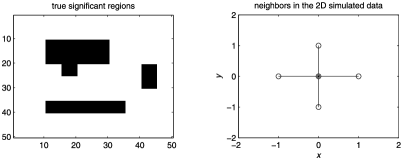
Figure 1: Left panel: the true significant regions for the $\mathrm{2D}$ simulated data sets. Right panel: neighbors of a point at $(x,y)$ used in the $\operatorname{FDR}_{L}$ procedure for $\mathrm{2D}$ simulated data.

Actual computations indicate that in this example, as long as $C>\log(4)$, $\alpha_{\infty}^{\operatorname{FDR}_{L}}$ is considerably smaller than $\alpha_{\infty}^{\operatorname{FDR}}$, indicating that the $\operatorname{FDR}_{L}$ procedure can adopt a control level much smaller than that of the conventional $\operatorname{FDR}$ procedure without excessively encountering the $\operatorname{LIP}$. For example, set $\lambda=0.1$; assume that the neighborhood in the $\operatorname{FDR}_{L}$ procedure is depicted in the right panel of Figure 1, that is, $k=5$. Table 2 compares values of $\alpha_{\infty}^{\operatorname{FDR}}$ and $\alpha_{\infty}^{\operatorname{FDR}_{L}}$ for $C=\log(4j)$, $j=2,\ldots,9$. Refer to (38) and (41) in Appendix C for detailed derivations of $\alpha_{\infty}^{\operatorname{FDR}}$ and $\alpha_{\infty}^{\operatorname{FDR}_{L}}$, respectively.

Table 2: Comparing $\vphantom{{{a^{\sum}}^{\int}}^{\sum}}\alpha_{\infty}^{\operatorname{FDR}}$ and $\alpha_{\infty}^{\operatorname{FDR}_{L}}$

$\bolds{C}$	$\bolds{\log(8)}$	$\bolds{\log(12)}$	$\bolds{\log(16)}$	$\bolds{\log(20)}$	$\bolds{\log(24)}$	$\bolds{\log(28)}$	$\bolds{\log(32)}$	$\bolds{\log(36)}$
$\alpha_{\infty}^{\operatorname{FDR}}$	0.4130	0.3043	0.2471	0.2079	0.1795	0.1579	0.1409	0.1273
$\alpha_{\infty}^{\operatorname{FDR}_{L}}$	0.0103	0.0030	0.0013	0.0007	0.0004	0.0002	0.0002	0.0001

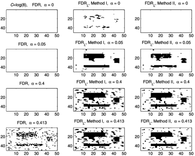
Figure 2: Lack of identification phenomenon when $\alpha$ varies from $0$ to $\alpha_{\infty}^{\operatorname{FDR}}=0.4130$. The sites that are called statistically significant based on the realization are shown in black. Left panels: the $\operatorname{FDR}$ procedure. Middle panels: the $\operatorname{FDR}_{L}$ procedure using Method $\mathrm{I}$. Right panels: the $\operatorname{FDR}_{L}$ procedure using Method $\mathrm{II}$.

To better visualize the $\operatorname{LIP}$ from limited data, Figure 2 compares the regions detected as significant by the $\operatorname{FDR}$ and $\operatorname{FDR}_{L}$ procedures for $C=\log(8)$ based on one realization of the simulated data. It is observed from Figure 2 that for $\alpha$ between $0$ and $0.4$, the $\operatorname{FDR}$ procedure lacks the ability to detect statistical significance; as $\alpha$ increases to $0.413$ (which is the limit $\alpha_{\infty}^{\operatorname{FDR}}=0.413$ as calculated in Table 2) and above, some significant results emerge. In contrast, for $\alpha$ close to $0$, both Method I and Method II for the $\operatorname{FDR}_{L}$ procedure are able to deliver some significant results. Similar plots to those in Figure 2 are obtained with other choices of $C$ and hence are omitted for lack of space.

5 Simulation study: 2D dependent data

5.1 Example $1$

To illustrate the distinction between the $\operatorname{FDR}_{L}$ and the conventional $\operatorname{FDR}$ procedures, we present simulation studies. The true significant regions are displayed as two black rectangles in the top left panel of Figure 3. The data are generated according to the model

$$Y(i,j)=\mu(i,j)+\varepsilon(i,j),\qquad i,j=1,\ldots,258,$$ (14)

where the signals are $\mu(i,j)=0$ for $(i,j)\in\mathcal{V}_{0}$, $\mu(i,j)=4$ in the larger black rectangle and $\mu(i,j)=2$ in the smaller black rectangle. The errors $\{\varepsilon(i,j)\}$ have zero-mean, unit-variance and are spatially dependent, by taking $\varepsilon(i,j)=\{e(i-1,j)+e(i,j)+e(i+1,j)+e(i,j-1)+e(i,j+1)\}/\sqrt{5}$, where $\{e(i,j)\}_{i,j=0}^{259}$ are i.i.d. $N(0,1)$. At each pixel $(i,j)$, $Y(i,j)$ is used as the test statistic for testing $\mu(i,j)=0$ against $\mu(i,j)>0$.

Both $\operatorname{FDR}$ and $\operatorname{FDR}_{L}$ procedures are preformed at a common control level $0.01$, with the tuning constant $\lambda=0.1$. In the $\operatorname{FDR}_{L}$ procedure, the neighborhood of a point at $(x,y)$ is taken as in the right panel of Figure 1. The histogram of the original $p$-values plotted in Figure 3(a) is flat except a sharp rise on the left border. The flatness is explained by the uniform distribution of the original $p$-values corresponding to the true null hypotheses, whereas the sharp rise is caused by the small $p$-values corresponding to the true alternative hypotheses. The histogram of the median aggregated $p^{*}$-values in Figure 3(c) shows a sharp rise at the left end and has a shape symmetric about $0.5$. The approximate symmetry arises from the limit distribution of $p^{*}$-values corresponding to the true null hypotheses [see (6)], whereas the sharp rise is formed by small $p^{*}$-values corresponding to the true alternative hypotheses. Figures 3(b), (d) and (d^′) manifest that the $\operatorname{FDR}$ procedure diminishes the effectiveness in detecting the significant regions than the $\operatorname{FDR}_{L}$ procedure, demonstrating that the $\operatorname{FDR}_{L}$ procedure more effectively increases the true positive rates. As a comparison, Figures 3(e), (f) and (f^′) correspond to using the mean (other than median) filter for aggregating $p$-values. It is seen that the detections by the median and mean filters are very similar; but compared with the mean, the median better preserves the edge of the larger black rectangle between significant and nonsignificant areas. This effect gets more pronounced when $\alpha$ increases, lending support to the “edge preservation property” of the median.

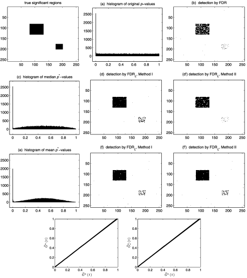
Figure 3: Comparison of the $\operatorname{FDR}$ and $\operatorname{FDR}_{L}$ procedures for Example $1$. In the first row, left: true significant regions shown in black; middle: histogram of the original $p$-values; right: significant regions detected by the $\operatorname{FDR}$ procedure. In the second row, left: histogram of the $p^{*}$-values using the median filter; middle and right: significant regions detected by the $\operatorname{FDR}_{L}$ procedure using Methods $\mathrm{I}$ and $\mathrm{II}$, respectively. In the third row, left: histogram of the $p^{*}$-values using the mean filter; middle and right: significant regions detected by the $\operatorname{FDR}_{L}$ procedure using Methods $\mathrm{I}$ and $\mathrm{II}$, respectively. In the bottom row, left: $\widehat{G}^{*}(t)$ versus $\widetilde{G}^{*}(t)$; right: $\widehat{G}_{c}^{*}(t)$ versus $\widetilde{G}^{*}(t)$; straight line: the $45$ degree reference line. Here $\alpha=0.01$ and $\lambda=0.1$.

To evaluate the performance of Method I and Method II in estimating $\widetilde{G}^{*}(t)$, the bottom panels of Figure 3 display the plots of $\widehat{G}^{*}(t)$ versus $\widetilde{G}^{*}(t)$ and $\widehat{G}^{*}_{c}(t)$ versus $\widetilde{G}^{*}(t)$. The agreement with 45 degree lines well supports both estimation methods.

To examine the overall performance of the estimated $\operatorname{FDR}(t)$ and $\operatorname{FDR}_{L}(t)$ for a same threshold $t\in[0,1]$, we replicate the simulation $100$ times. For notational convenience, denote by $\operatorname{FDP}(t)=V(t)/\{R(t)\vee 1\}$ and $\operatorname{FDP}_{L}(t)=V^{*}(t)/\{R^{*}(t)\vee 1\}$ the false discovery proportions of the $\operatorname{FDR}$ and $\operatorname{FDR}_{L}$ procedures, respectively. The average values (over $100$ data) of $\widehat{\operatorname}{FDR}(t)$ and $\widehat{\operatorname}{FDR}_{L}(t)$ at each point $t$ are plotted in Figure 4(a).

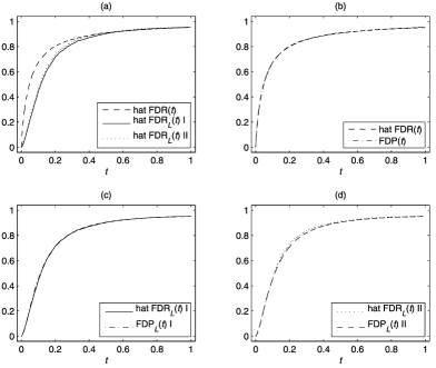
Figure 4: Panel (a): compare the average values of $\widehat{\operatorname}{FDR}(t)$ and those of $\widehat{\operatorname}{FDR}_{L}(t)$ using Methods $\mathrm{I}$ and $\mathrm{II}$. Panel (b): compare the average values of $\widehat{\operatorname}{FDR}(t)$ and those of $\operatorname{FDP}(t)$. Panel (c): compare the average values of $\widehat{\operatorname}{FDR}_{L}(t)$ using Method $\mathrm{I}$ and those of $\operatorname{FDP}_{L}(t)$. Panel (d): compare the average values of $\widehat{\operatorname}{FDR}_{L}(t)$ using Method $\mathrm{II}$ and those of $\operatorname{FDP}_{L}(t)$. Here $\lambda=0.1$.

It is clearly observed that $\widehat{\operatorname}{FDR}_{L}(t)$ using both Methods $\mathrm{I}$ and $\mathrm{II}$ is below $\widehat{\operatorname}{FDR}(t)$, demonstrating that the $\operatorname{FDR}_{L}$ procedure produces the estimated false discovery rates lower than those of the $\operatorname{FDR}$ procedure. Meanwhile, Figure 4 compares the average values of $\operatorname{FDP}(t)$ and those of $\widehat{\operatorname}{FDR}(t)$ in panel (b), and the average values of $\operatorname{FDP}_{L}(t)$ using Methods $\mathrm{I}$ and $\mathrm{II}$ and those of $\widehat{\operatorname}{FDR}_{L}(t)$ in panels (c) and (d), respectively. For each procedure, the two types of estimates are very close to each other, lending support to the estimation procedure in Section 3.4.

5.1.1 Sensitivity and specificity

To further study the relative performance of the $\operatorname{FDR}$ and $\operatorname{FDR}_{L}$ procedures, we adopt two widely used performance measures,

$$\mathrm{sensitivity} \equiv \cases{{S(t_{\alpha}(\widehat{\operatorname}{FDR}))}/{n_{1}},&\quad\mbox{for the $\operatorname{FDR}$ procedure},\cr{S^{*}(t_{\alpha}(\widehat{\operatorname}{FDR}_{L}))}/{n_{1}},&\quad\mbox{for the $\operatorname{FDR}_{L}$ procedure},}$$

$$\mathrm{specificity} \equiv \cases{{U(t_{\alpha}(\widehat{\operatorname}{FDR}))}/{n_{0}},&\quad\mbox{for the $\operatorname{FDR}$ procedure},\cr{U^{*}(t_{\alpha}(\widehat{\operatorname}{FDR}_{L}))}/{n_{0}},&\quad\mbox{for the $\operatorname{FDR}_{L}$ procedure},}$$

for summarizing the discriminatory power of a diagnosis procedure, where $S(t)=\sum_{i=1}^{n}\mathrm{I}\{H_{0}(i)$ is false, and $p_{i}\leq t\}$, $U(t)=\sum_{i=1}^{n}\mathrm{I}\{H_{0}(i)$ is true, and $p_{i}>t\}$, $S^{*}(t)=\sum_{i=1}^{n}\mathrm{I}\{H_{0}(i)$ is false, and $p_{i}^{*}\leq t\}$ and $U^{*}(t)=\sum_{i=1}^{n}\mathrm{I}\{H_{0}(i)$ is true, and $p_{i}^{*}>t\}$. Here, the sensitivity and specificity measure the strengths for correctly identifying the alternative and the null hypotheses, respectively.

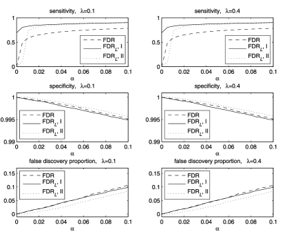
Figure 5: Comparison of the average sensitivity (top panels), average specificity (middle panels) and average false discovery proportion (bottom panels). Left panels: $\lambda=0.1$. Right panels: $\lambda=0.4$.

Following Section 5.1, we randomly generate $100$ sets of simulated data and perform $\operatorname{FDR}$ and $\operatorname{FDR}_{L}$ procedures for each dataset, with the control levels $\alpha$ varying from $0$ to $0.1$. The left panel of Figure 5 corresponds to $\lambda=0.1$, whereas the right panel corresponds to $\lambda=0.4$. In either case, we observe that the average sensitivity (over the datasets) of the $\operatorname{FDR}_{L}$ procedure using Method I is consistently higher than that of the $\operatorname{FDR}$ procedure, whereas the average specificities of both procedures approach one and are nearly indistinguishable. In addition, the bottom panels indicate that the $\operatorname{FDR}$ procedure yields larger (average) false discovery proportions than the $\operatorname{FDR}_{L}$ procedure. It is apparent that the results in Figure 5 are not very sensitive to the choice of $\lambda$. Unless otherwise stated, $\lambda=0.1$ will be used throughout the rest of the numerical work.

5.2 Example $2$: More strongly correlated case

We consider a dataset generated according to the same model (14) as in Example 1, but with more strongly correlated errors, by taking $\varepsilon(i,j)=\sum_{i=0}^{6}\sum_{j=0}^{6}e(i,j)/7$, where $\{e(i,j)\}_{i,j=0}^{264}$ are i.i.d. $N(0,1)$. As seen from the figure in Zhang, Fan and Yu (2010), both $\operatorname{FDR}$ and $\operatorname{FDR}_{L}$ (using Methods I and II) procedures perform worse with strongly-correlated data than with low-correlated data (given in Figure 3). However, there are no adverse effects by applying $\operatorname{FDR}_{L}$ to more strongly correlated data, and Method I continues to be comparable with Method II for the $\operatorname{FDR}_{L}$ procedure.

5.3 Example $3$: Large proportion of boundary grid points

The efficacy of the $\operatorname{FDR}_{L}$ procedure is illustrated in the figure of Zhang, Fan and Yu (2010) by a simulated dataset generated according to the same model (14) as in Example 1, but with a large proportion of boundary grid points, where $\mu(i,j)=0$ for $(i,j)\in\mathcal{V}_{0}$ and $\mu(i,j)=4$ for $(i,j)\in\mathcal{V}_{1}$. Similar plots using $\mu(i,j)=2$ for $(i,j)\in\mathcal{V}_{1}$ are obtained and thus omitted. Again, there is no adverse effect of using $\operatorname{FDR}_{L}$ to detect dense or weak signals.

6 Simulation study: 3D dependent data

We apply the $\operatorname{FDR}$ and $\operatorname{FDR}_{L}$ procedures to detect activated brain regions of a simulated brain fMRI dataset, which is both spatially and temporally correlated. The experiment design, timings and size are exactly the same as those of the real fMRI dataset in Section 7.

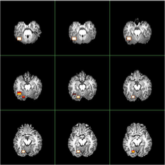
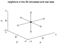
Figure 6: Left panel: true activated brain regions (denoted by hot color) for the simulated $\operatorname{fMRI}$ dataset. Right panel: neighbors of a point at $(x,y,z)$ used in the $\operatorname{FDR}_{L}$ procedure for $\mathrm{3D}$ simulated and real data.

The data are generated from a semi-parametric model similar to that in Section 5.2 of Zhang and Yu (2008). (They demonstrated that the semi-parametric model gains more flexibilities than existing parametric models.) The left panel of Figure 6 contains $9$ slices (corresponding to the 2D axial view) which highlight two activated brain regions involving $91$ activated brain voxels. The neighborhood used in the $\operatorname{FDR}_{L}$ procedure is illustrated in the right panel of Figure 6.

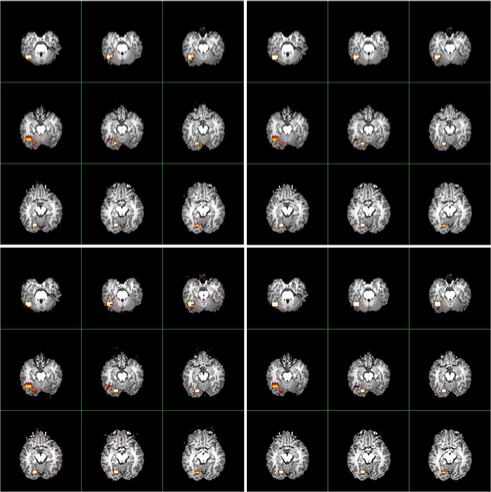
Figure 7: Comparison of activated brain regions detected for the simulated $\operatorname{fMRI}$ dataset using the conventional $\operatorname{FDR}$ approach (on the left) and the proposed $\operatorname{FDR}_{L}$ procedure (on the right) using Method $\mathrm{I}$. Top panels: $\mathbb{K}$. Bottom panels: $\mathbb{K}_{\mathrm{bc}}$. Here $\alpha=0.05$.

Figure 7 compares the activated brain regions identified by the $\operatorname{FDR}$ (in the left panels) and $\operatorname{FDR}_{L}$ (in the right panels) procedures. Owing to the wealth of data, and for purposes of computational simplicity, results using Method I of $\operatorname{FDR}_{L}$ are presented. Voxel-wise inactivity is tested with the semi-parametric test statistics $\mathbb{K}=(A\widehat{\mathbf{h}})^{T}\{A(\widetilde{\mathbf{S}}^{T}\widehat{R}^{-1}\widetilde{\mathbf{S}})^{-1}A^{T}\}^{-1}(A\widehat{\mathbf{h}})/\break\{\widehat{\mathbf{r}}^{T}\widehat{R}^{-1}\widehat{\mathbf{r}}/(n-rm)\}$ (in the top panels) and $\mathbb{K}_{\mathrm{bc}}=(A\widehat{\mathbf{h}}_{\mathrm{bc}})^{T}\{A(\widetilde{\mathbf{S}}^{T}\widehat{R}^{-1}\widetilde{\mathbf{S}})^{-1}\*A^{T}\}^{-1}(A\widehat{\mathbf{h}}_{\mathrm{bc}})/\{\widehat{\mathbf{r}}_{\mathrm{bc}}^{T}\widehat{R}^{-1}\widehat{\mathbf{r}}_{\mathrm{bc}}/(n-rm)\}$ (in the bottom panels) whose notation was given and asymptotic $\chi^{2}$ distributions were derived in Zhang and Yu (2008). The control level is $0.05$. Inspection of Figure 7 reveals that $\mathbb{K}$ and $\mathbb{K}_{\mathrm{bc}}$ locate both active regions. In particular, using the $\operatorname{FDR}$ procedure, both methods detect more than $200$ voxels (which are visible when zooming the images), many of which are falsely discovered. When applying the $\operatorname{FDR}_{L}$ procedure, $\mathbb{K}$ detects $82$ voxels, whereas $\mathbb{K}_{\mathrm{bc}}$ detects $90$ voxels. Thus the $\operatorname{FDR}_{L}$ procedure reduces the number of tiny scattered false findings, gaining more accurate detections than the $\operatorname{FDR}$ procedure.

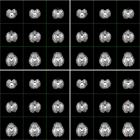
Figure 8: Comparison of activated brain regions detected for the simulated $\operatorname{fMRI}$ dataset using the conventional $\operatorname{FDR}$ approach (on the left) and the proposed $\operatorname{FDR}_{L}$ procedure (on the right) using Method $\mathrm{I}$. Top panels: $\operatorname{AFNI}$. Bottom panels: $\operatorname{FSL}$. Here $\alpha=0.05$.

As a comparison, the detection results by popular software AFNI [Cox (1996)] and FSL [Smith et al. (2004) and Woolrich et al. (2001)] are given in Figure 8. We observe that both AFNI and FSL fail to locate one activated brain area, and that the other region, though correctly detected, has appreciably reduced size relative to the actual size. This detection bias is due to the stringent assumptions underlying AFNI and FSL in modeling fMRI data: the Hemodynamic Response Function (HRF) in FSL is specified as the difference of two gamma functions, and the drift term in AFNI is specified as a quadratic polynomial. As anticipated, applying the $F$ distributions restricted to parametric models to specify the distributions of test statistics in AFNI and FSL leads to bias, which in turn gives biased calculations of $p$-values and $p^{*}$-values. In this case, the detection performances of both the $\operatorname{FDR}$ and $\operatorname{FDR}_{L}$ procedures deteriorate, and the $\operatorname{FDR}_{L}$ procedure does not improve the performance of the $\operatorname{FDR}$ procedure. See Table 3 for a more detailed comparison.

To reduce modeling bias, for applications to the real fMRI dataset in Section 7, we will only employ the semi-parametric test statistics $\mathbb{K}$ and $\mathbb{K}_{\mathrm{bc}}$. It is also worth distinguishing between the computational aspects associated with the $\operatorname{FDR}_{L}$ procedure: this paper uses (7) for the null distribution of $p^{*}$-values, whereas Zhang and Yu (2008) used the normal approximation approach in Section 3.2.

7 Functional neuroimaging example

In an emotional control study, subjects saw a series of negative or positive emotional images, and were asked to either suppress or enhance their emotional responses to the image, or to simply attend to the image. The sequence of trials was randomized. The time between successive trials also varied. The size of the whole brain dataset is $64\times 64\times 30$. At each voxel, the time series has $6$ runs, each containing $185$ observations with a time resolution of $2$ seconds. For details of the dataset, please refer to Zhang and Yu (2008). The study aims to estimate the BOLD (Blood Oxygenation Level-Dependent) response to each of the trial types for $1$–$18$ seconds following the image onset. We analyze the fMRI dataset containing one subject. The length of the estimated HRF is set equal to $18$. Again, the neighborhood used in the $\operatorname{FDR}_{L}$ procedure is illustrated in the right panel of Figure 6.

Table 3: Comparing ${\operatorname{FDR}}$ and ${\operatorname{FDR}_{L}}$ procedures

		Test methods
	Multiple comparison	$\bolds{\mathbb{K}}$	$\bolds{\mathbb{K}_{\mathrm{bc}}}$	AFNI	FSL
# of detected voxels	$\operatorname{FDR}$	$276$	$870$	$16$	$6$
	$\operatorname{FDR}_{L}$, Method I	$82$	$90$	$2$	$11$
False discovery proportion	$\operatorname{FDR}$	$0.6993$	$0.9000$	$0.5625$	$0$
	$\operatorname{FDR}_{L}$, Method I	$0$	$0$	$0.5000$	$0$
Sensitivity	$\operatorname{FDR}$	$0.9121$	$0.9560$	$0.0769$	$0.0659$
	$\operatorname{FDR}_{L}$, Method I	$0.9011$	$0.9890$	$0.0110$	$0.1209$
Specificity	$\operatorname{FDR}$	$0.9921$	$0.9678$	$0.9996$	$1.0000$
	$\operatorname{FDR}_{L}$, Method I	$1.0000$	$1.0000$	$0.9997$	$1.0000$

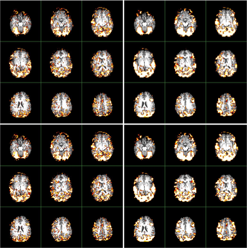
Figure 9: Comparison of activated brain regions detected for the real $\operatorname{fMRI}$ dataset using the conventional $\operatorname{FDR}$ approach (on the left) and the proposed $\operatorname{FDR}_{L}$ procedure (on the right) using Method $\mathrm{I}$. Top panels: $\mathbb{K}$. Bottom panels: $\mathbb{K}_{\mathrm{bc}}$. Here $\alpha=0.001$.

A comparison of the activated brain regions using the $\operatorname{FDR}$ and $\operatorname{FDR}_{L}$ procedures is visualized in Figure 9. The level $0.001$ is used to carry out the multiple comparisons. The conventional $\operatorname{FDR}$ procedure finds more tiny scattered active voxels, which are more likely to be falsely discovered. In contrast, the $\operatorname{FDR}_{L}$ procedure finds activation in much more clustered regions of the brain.

8 Discussion

This paper proposes the $\operatorname{FDR}_{L}$ procedure to embed the structural spatial information of $p$-values into the conventional $\operatorname{FDR}$ procedure for large-scale imaging data with a spatial structure. This procedure provides the standard $\operatorname{FDR}$ procedure with the ability to perform better on spatially aggregated $p$-values. Method I and Method II have been developed for making statistical inference of the aggregated $p$-values under the null. Method I gains remarkable computational superiority, particularly for large/huge imaging datasets, when the $p^{*}$-values under the null are not too skewed. Furthermore, we provide a better understanding of a “lack of identification phenomenon” ($\operatorname{LIP}$) occurring in the $\operatorname{FDR}$ procedure. This study indicates that the $\operatorname{FDR}_{L}$ procedure alleviates the extent of the problem and can adopt control levels much smaller than those of the $\operatorname{FDR}$ procedure without excessively encountering the $\operatorname{LIP}$, thus substantially facilitating the selection of more stringent control levels.

As discussed in Owen (2005) and Leek and Storey (2008), a key issue with the dependencies between the hypotheses tests is the inflation of the variance of significance measures in $\operatorname{FDR}$-related work. Indeed, similar to $\operatorname{FDR}$, the $\operatorname{FDR}_{L}$ procedure (using Methods I and II) performs less well with highly-correlated data than with the low-correlated data. Detailed investigation of the variance of $\operatorname{FDR}_{L}$ will be given in future study.

Other ways of exploring spatially neighboring information are certainly possible in multiple comparison. For example, the median operation applied to $p$-values can be replaced by the averaging, kernel smoothing, “majority vote” and edge preserving smoothing techniques [Chu et al. (1998)]. Hence, taking the median is not the unique way to aggregate $p$-values. On the other hand, compared with the mean, the median is more robust, computationally simpler and does not depend excessively on the spatial co-ordinates, especially on the boundaries between significant and nonsignificant regions, as observed in Figures 3(d) and (f). An exhaustive comparison is beyond the scope of the current paper and we leave this for future research.

Appendix A Proofs of Theorems 4.1–4.3

We first impose some technical assumptions, which are not the weakest possible. Detailed proofs of Theorems 4.1–4.3 are given in Zhang, Fan and Yu (2010).

Condition A.

The neighborhood size $k$ is an integer not depending on $n$.

limn→∞n0/n=π0 exists and $\pi_{0}<1$.

limn→∞V∗(t)/n0=G0∗(t) and $\lim_{n\to\infty}{S^{*}(t)}/{n_{1}}=G_{1}^{*}(t)$ almost surely for each $t\in(0,1]$, where $G_{0}^{*}$ and $G_{1}^{*}$ are continuous functions.

0<G0∗(t)≤G∗∞(t) for each $t\in(0,1]$.

supt∈(0,1]|^G∗(t)-G∗∞(t)|=o(1) almost surely as $n\to\infty$.

Appendix B Proofs of Theorems 4.4 and 4.5

B.1 Proof of Theorem 4.4

By the assumptions and $H_{1}(v)$, we see that the $p$-value has the expression, $p(v)=1-F_{0}(T(v))$. Thus, the distribution function of $p(v)$ corresponding to the true $H_{0}(v)$ is $G_{0}(t)=t$ for $0<t<1$ and (3) gives $\widehat{\operatorname{FDR}}^{\infty}(t)=\frac{\pi_{0}+\pi_{1}\{1-G_{1}(\lambda)\}/(1-\lambda)}{\pi_{0}+\pi_{1}G_{1}(t)/t}$. Also, the distribution function of $p(v)$ corresponding to the true $H_{1}(v)$ is given by

$$G_{1}(t)=1-F_{1}\bigl{(}F_{0}^{-1}(1-t)\bigr{)}.$$ (15)

Likewise, using (6), it follows that with probability one,

$$G_{0}^{*}(t) = \lim_{n\to\infty}\frac{V^{*}(t)}{n_{0}}$$

$$= \lim_{n\to\infty}\frac{\sum_{v\in\mathcal{V}_{0}^{(0)}}\mathrm{I}\{p^{*}(v)\leq t\}}{\#\mathcal{V}_{0}^{(0)}}\cdot\lim_{n\to\infty}\frac{\#\mathcal{V}_{0}^{(0)}}{n_{0}}$$

$${}+\lim_{n\to\infty}\frac{\sum_{v\in\mathcal{V}_{0}\setminus\mathcal{V}_{0}^{(0)}}\mathrm{I}\{p^{*}(v)\leq t\}}{n_{0}}$$

$$= P\{p^{*}(v)\leq t\}\qquad\mbox{with }v\in\mathcal{V}_{0}^{(0)}$$

$$= G^{*\infty}(t)=B_{(k+1)/2,(k+1)/2}(t),$$

the cumulative distribution function of a ${\operatorname{Beta}}((k+1)/2,(k+1)/2)$ random variable and

$$G_{1}^{*}(t)=\lim_{n\to\infty}{S^{*}(t)}/{n_{1}}=B_{(k+1)/2,(k+1)/2}(G_{1}(t)).$$ (17)

Applying (B.1) and (12) gives $\widehat{\operatorname}{FDR}_{L}^{\infty}(t)=\frac{\pi_{0}+\pi_{1}\{1-G_{1}^{*}(\lambda)\}/\{1-G_{0}^{*}(\lambda)\}}{\pi_{0}+\pi_{1}G_{1}^{*}(t)/G_{0}^{*}(t)}$.

Part I. For the $\operatorname{FDR}$ procedure, note that $\widehat{\operatorname{FDR}}^{\infty}(t)$ is a decreasing function of $G_{1}(t)/t$. Applying L’Hospital’s rule and the fact $\lim_{t\to 0+}G_{1}(t)=0$,

$$\lim_{t\to 0+}\frac{G_{1}(t)}{t}=\lim_{t\to 0+}\frac{f_{1}(F_{0}^{-1}(1-t))}{f_{0}(F_{0}^{-1}(1-t))}=\lim_{x\to x_{0}-}\frac{f_{1}(x)}{f_{0}(x)}=\infty,$$ (18)

where $x=F_{0}^{-1}(1-t)$. Thus, $\sup_{0<t\leq 1}G_{1}(t)/t=\infty$, which together with $\widehat{\operatorname{FDR}}^{\infty}(t)$ shows $\alpha_{\infty}^{\operatorname{FDR}}=0$ for the $\operatorname{FDR}$ procedure.

For the $\operatorname{FDR}_{L}$ procedure, applying (B.1) and (17), we get

$$\qquad\frac{dG_{0}^{*}(t)}{dt} = \frac{dG^{*\infty}(t)}{dt}=\frac{k!}{[\{(k-1)/2\}!]^{2}}t^{(k-1)/2}(1-t)^{(k-1)/2},$$ (19)

$$\frac{dG_{1}^{*}(t)}{dt} = \frac{k!}{[\{(k-1)/2\}!]^{2}}G_{1}(t)^{(k-1)/2}\{1-G_{1}(t)\}^{(k-1)/2}\,\frac{dG_{1}(t)}{dt}.$$ (20)

Note that $\widehat{\operatorname}{FDR}_{L}^{\infty}(t)$ is a decreasing function of $G_{1}^{*}(t)/G_{0}^{*}(t)$. Since$\lim_{t\to 0+}G_{1}^{*}(t)=0$ and $\lim_{t\to 0+}G_{0}^{*}(t)=0$,

$$\lim_{t\to 0+}\frac{G_{1}^{*}(t)}{G_{0}^{*}(t)} = \lim_{t\to 0+}\frac{{dG_{1}^{*}(t)}/{dt}}{{dG_{0}^{*}(t)}/{dt}}$$

$$= \lim_{t\to 0+}\biggl{\{}\frac{G_{1}(t)}{t}\cdot\frac{1-G_{1}(t)}{1-t}\biggr{\}}^{(k-1)/2}\,\frac{dG_{1}(t)}{dt},$$

which together with (18) shows $\lim_{t\to 0+}G_{1}^{*}(t)/G_{0}^{*}(t)=\infty$. Thus,

$$\sup_{0<t\leq 1}G_{1}^{*}(t)/G_{0}^{*}(t)=\infty,$$

that is, $\alpha_{\infty}^{\operatorname{FDR}_{L}}=0$ for the $\operatorname{FDR}_{L}$ procedure.

Part II. Following $\widehat{\operatorname{FDR}}^{\infty}(t)$ and $\widehat{\operatorname}{FDR}_{L}^{\infty}(t)$, we immediately conclude that $\alpha_{\infty}^{\operatorname{FDR}}\neq 0$ if

$$\sup_{0<t\leq 1}G_{1}(t)/t<\infty,$$ (22)

and that $\alpha_{\infty}^{\operatorname{FDR}_{L}}\neq 0$ if

$$\sup_{0<t\leq 1}G_{1}^{*}(t)/G_{0}^{*}(t)<\infty.$$ (23)

We first verify (22) for the $\operatorname{FDR}$ procedure. Assume (22) fails, that is, $\sup_{0<t\leq 1}G_{1}(t)/t=\infty$. Note that for any $\delta>0$, the function $G_{1}(t)/t$, for $t\in[\delta,1]$, is continuous and bounded away from $\infty$, thus, $\sup_{0<t\leq 1}G_{1}(t)/t=\infty$ only if there exists a sequence $t_{1}>t_{2}>\cdots>0$, such that $\lim_{m\to\infty}t_{m}=0$ and $\lim_{m\to\infty}G_{1}(t_{m})/t_{m}=\infty$. For each $m$, recall that both $G_{1}(t)$ and $t$ are continuous on $[0,t_{m}]$, and differentiable on $(0,t_{m})$. Applying Cauchy’s mean-value theorem, there exists $\xi_{m}\in(0,t_{m})$ such that ${G_{1}(t_{m})}/{t_{m}}=\{G_{1}(t_{m})-G_{1}(0)\}/{(t_{m}-0)}=\frac{dG_{1}(t)}{dt}|_{t=\xi_{m}}.$ Since $\lim_{m\to\infty}G_{1}(t_{m})/t_{m}=\infty$, it follows that

$$\limsup_{t\to 0+}\frac{dG_{1}(t)}{dt}=\infty.$$ (24)

On the other hand, the condition $\limsup_{x\to x_{0}-}\frac{f_{1}(x)}{f_{0}(x)}<\infty$ indicates that

$$\quad\limsup_{t\to 0+}\frac{dG_{1}(t)}{dt}=\limsup_{t\to 0+}\frac{f_{1}(F_{0}^{-1}(1-t))}{f_{0}(F_{0}^{-1}(1-t))}=\limsup_{x\to x_{0}-}\frac{f_{1}(x)}{f_{0}(x)}<\infty,$$ (25)

where $x=F_{0}^{-1}(1-t)$. Clearly, (25) contradicts (24).

Next, we show (23) for the $\operatorname{FDR}_{L}$ procedure. Combining (B.1), (22) and (25), the result follows. This completes the proof.

B.2 Proof of Theorem 4.5

We first show Lemma 1.

Lemma 1

Let $B(t)$ be the cumulative distribution function of a ${\operatorname{Beta}}(a,a)$ random variable, where $a>1$ is a real number. Then $\mathrm{I}$ for $t\in(0,0.5)$, $B(t)/t$ is a strictly increasing function and $B(t)<t$; $\mathrm{II}$ for $t\in(0.5,1)$, $B(t)>t$; $\mathrm{III}$ for $t_{1}\in(0,0.5]$ and $t_{2}\in[t_{1},1]$, $B(t_{1})/t_{1}\leq B(t_{2})/t_{2}$.

Let $\Gamma(\cdot)$ denote the Gamma function. It is easy to see that

$$B^{\prime\prime}(t)={\Gamma(2a)}/{\{\Gamma(a)\}^{2}}(a-1)t^{a-2}(1-t)^{a-2}(1-2t).$$ (26)

To show part I, define $F_{1}(t)=B(t)/t$. Then $F_{1}^{\prime}(t)=\{B^{\prime}(t)t-B(t)\}/t^{2}$, where $\frac{d\{B^{\prime}(t)t-B(t)\}}{dt}=B^{\prime\prime}(t)t$. For $t\in(0,0.5)$, (26) indicates $B^{\prime\prime}(t)>0$, that is, $B^{\prime}(t)t-B(t)$ is strictly increasing, implying $B^{\prime}(t)t-B(t)>B^{\prime}(0)0-B(0)=0$. Hence for $t\in(0,0.5)$, $B(t)/t$ is strictly increasing, and therefore $B(t)/t<B(0.5)/0.5=1$.

For part II, define $F_{2}(t)=B(t)-t$. Then $F_{2}^{\prime\prime}(t)=B^{\prime\prime}(t)$. By (26), $B^{\prime\prime}(t)<0$ for $t\in(0.5,1)$, thus $F_{2}(t)$ is strictly concave, giving $F_{2}(t)>\max\{F_{2}(0.5)$, $F_{2}(1)\}=0$.

Last, we show part III. For $t_{2}\in[t_{1},0.5]$, part I indicates that $B(t_{1})/t_{1}\leq B(t_{2})/t_{2}$; for $t_{2}\in[0.5,1]$, part II indicates that $B(t_{2})/t_{2}\geq 1$ which, combined with $B(t_{1})/t_{1}\leq 1$ from part I, yields $B(t_{1})/t_{1}\leq B(t_{2})/t_{2}$.

We now prove Theorem 4.5. It suffices to show that

$$\{1-G_{1}(\lambda)\}/{(1-\lambda)} \geq \{1-G_{1}^{*}(\lambda)\}/\{1-G_{0}^{*}(\lambda)\},$$ (27)

$$\sup_{0<t\leq 1}{G_{1}(t)}/{t} \leq \sup_{0<t\leq 1}{G_{1}^{*}(t)}/{G_{0}^{*}(t)}.$$ (28)

Following (19) and (20), for $0\leq t\leq 1$,

$$G_{1}^{*}(t)=G_{0}^{*}(G_{1}(t)).$$ (29)

Applying (29), (15), $1-F_{0}(F_{1}^{-1}(0.5))\leq\lambda$ and part II of Lemma 1 yields $G_{1}(\lambda)\leq G_{1}^{*}(\lambda)$; applying $\lambda\leq 0.5$ and part I of Lemma 1 implies $\lambda\geq G_{0}^{*}(\lambda)$. This shows (27).

To verify (28), let $M=\sup_{0<t\leq 1}{G_{1}(t)}/{t}$. Since $G_{1}(1)/1=1$, we have $M\geq 1$ which will be discussed in two cases. Case 1: if $M=1$, then

$$\sup_{0<t\leq 1}\frac{G_{1}^{*}(t)}{G_{0}^{*}(t)}\geq\frac{G_{1}^{*}(1)}{G_{0}^{*}(1)}=1=\sup_{0<t\leq 1}\frac{G_{1}(t)}{t}.$$ (30)

Case 2: if $M>1$, then there exists $t_{0}\in[0,1]$ and $t_{n}\in(0,1)$ such that $\lim_{n\to\infty}t_{n}=t_{0}$, and

$$\lim_{n\to\infty}G_{1}(t_{n})/t_{n}=\sup_{0<t\leq 1}G_{1}(t)/t=M>1.$$ (31)

Thus, there exists $N_{1}$ such that for all $n>N_{1}$,

$$G_{1}(t_{n})>t_{n}.$$ (32)

Cases of $t_{0}=1$, $t_{0}=0$ and $t_{0}\in(0,1)$ will be discussed separately. First, if $t_{0}=1$, then $M=\lim_{n\to\infty}G_{1}(t_{n})/t_{n}=\lim_{n\to\infty}G_{1}(t_{n})\leq 1$, which contradicts (31). Thus $t_{0}<1$. Second, if $t_{0}=0$, then there exists $N_{2}$ such that $t_{n}<0.5$ for all $n>N_{2}$. Thus for all $n>N\equiv\max\{N_{1},N_{2}\}$, applying (29), (32) and part III of Lemma 1, we have that

$$\frac{G_{1}^{*}(t_{n})}{G_{1}(t_{n})}=\frac{G_{0}^{*}(G_{1}(t_{n}))}{G_{1}(t_{n})}\geq\frac{G_{0}^{*}(t_{n})}{t_{n}}.$$

This together with (31) shows

$$\qquad\sup_{0<t\leq 1}\frac{G_{1}^{*}(t)}{G_{0}^{*}(t)}\geq\limsup_{n\to\infty}\frac{G_{1}^{*}(t_{n})}{G_{0}^{*}(t_{n})}\geq\lim_{n\to\infty}\frac{G_{1}(t_{n})}{t_{n}}=M=\sup_{0<t\leq 1}\frac{G_{1}(t)}{t}.$$ (33)

Third, for $t_{0}\in(0,1)$, since both $F_{0}$ and $F_{1}$ are differentiable and $f_{0}$ is supported in a single interval, $G_{1}(t)/t=\{1-F_{1}(F_{0}^{-1}(1-t))\}/t$ is differentiable in $(0,1)$. Thus,

$$\sup_{0<t\leq 1}{G_{1}(t)}/{t}={G_{1}(t_{0})}/{t_{0}}=M$$ (34)

and $\frac{d\{G_{1}(t)/t\}}{dt}|_{t=t_{0}}=0$. Notice

$$\frac{d\{G_{1}(t)/t\}}{dt}\bigg{|}_{t=t_{0}} = \frac{({dG_{1}(t)}/{dt})|_{t=t_{0}}-G_{1}(t_{0})/t_{0}}{t_{0}}$$

$$= \frac{({dG_{1}(t)}/{dt})|_{t=t_{0}}-M}{t_{0}}=0.$$

If $t_{0}>0.5$, then $F_{0}^{-1}(1-t_{0})\leq F_{0}^{-1}(0.5)$. By (18) and the assumption on $f_{0}$ and $f_{1}$, $\frac{dG_{1}(t)}{dt}|_{t=t_{0}}=f_{1}(F_{0}^{-1}(1-t_{0}))/f_{0}(F_{0}^{-1}(1-t_{0}))\leq 1$, which contradicts (B.2). Thus, $0<t_{0}\leq 0.5$. This together with (29), (34), and part III of Lemma 1 gives

$$\frac{G_{1}^{*}(t_{0})}{G_{1}(t_{0})}=\frac{G_{0}^{*}(G_{1}(t_{0}))}{G_{1}(t_{0})}\geq\frac{G_{0}^{*}(t_{0})}{t_{0}}.$$

This, together with (34), shows

$$\sup_{0<t\leq 1}\frac{G_{1}^{*}(t)}{G_{0}^{*}(t)}\geq\frac{G_{1}^{*}(t_{0})}{G_{0}^{*}(t_{0})}\geq\frac{G_{1}(t_{0})}{t_{0}}=M=\sup_{0<t\leq 1}\frac{G_{1}(t)}{t}.$$ (36)

Combining (30), (33) and (36) completes the proof.

Appendix C $\alpha_{\infty}^{\operatorname{FDR}}$ and $\alpha_{\infty}^{\operatorname{FDR}_{L}}$ in Table 2 of Section 4.3

Before calculating $\alpha_{\infty}^{\operatorname{FDR}}$ and $\alpha_{\infty}^{\operatorname{FDR}_{L}}$, we first present two lemmas.

Lemma 2

Let $f(x)$ and $g(x)$ be differentiable functions in $x\in(a,b)\subseteq\mathbb{R}$. Suppose that $g(x)\neq 0$ for $x\in(a,b)$, and $f(x)/g(x)$ is a nonincreasing function of $x$. For any $C\in(0,\infty)$ such that $g(x)+C\neq 0$, if ${df(x)}/{dx}\leq{dg(x)}/{dx}$ for all $x\in(a,b)$, then $\{f(x)+C\}/\{g(x)+C\}$ is a decreasing function in $x\in(a,b)$.

The proof is straightforward and is omitted.

Lemma 3

The function $h(x)={(10-15e^{C}x+6e^{2C}x^{2})}/{(10-15x+6x^{2})}$ is decreasing in $x\in(0,e^{-C})$, for any constant $C\in(\log(4),\infty)$.

The function $h(x)$ can be rewritten as $h(x)=\{6(-e^{C}x+5/4)^{2}+5/8\}/\{6(-x+5/4)^{2}+5/8\}$. Note that $(-e^{C}x)/(-x)=e^{C}$ is nonincreasing in $x$ and $e^{C}>1$ for $x>0$. Applying Lemma 2, $(-e^{C}x+5/4)/(-x+5/4)$ is decreasing in $x\in(0,e^{-C})$, so is $(-e^{C}x+5/4)^{2}/(-x+5/4)^{2}$. When $C>\log(4)$, ${d\{(-e^{C}x+5/4)^{2}\}}/{dx}\leq{d\{(-x+5/4)^{2}\}}/{dx}$. This together with Lemma 2 verifies that $h(x)$ is decreasing in $x\in(0,e^{-C})$.

First, we evaluate $\alpha_{\infty}^{\operatorname{FDR}}$. From (15) and the conditions in Section 4.3,

$$G_{0}(t)=t\qquad\mbox{for }t\in[0,1]\quad\mbox{and}\quad G_{1}(t)=\cases{te^{C},&\quad if $t\in[0,e^{-C}]$,\cr 1,&\quad if $t\in(e^{-C},1]$.}$$ (37)

Thus $\sup_{0<t\leq 1}G_{1}(t)/t=e^{C}$. By $\widehat{\operatorname{FDR}}^{\infty}(t)$ in Appendix B,

$$\alpha_{\infty}^{\operatorname{FDR}}=\frac{\pi_{0}+\pi_{1}\{1-\lambda e^{C}\mathrm{I}(\lambda<e^{-C})-\mathrm{I}(\lambda\geq e^{-C})\}/(1-\lambda)}{\pi_{0}+\pi_{1}e^{C}}.$$ (38)

Next, we compute $\alpha_{\infty}^{\operatorname{FDR}_{L}}$. Recall from Appendix B that the distribution $G_{0}^{*}(t)$ with $k=5$ is that of a $\operatorname{Beta}(3,3)$ random variable. Similarly, by (37), the distribution $G_{1}^{*}(t)$ is that of a $\operatorname{Beta}(3,3)/e^{C}$ random variable. By $\widehat{\operatorname}{FDR}_{L}^{\infty}(t)$ in Appendix B, $\widehat{\operatorname}{FDR}_{L}^{\infty}(t)$ is a decreasing function of $G_{1}^{*}(t)/G_{0}^{*}(t)$, for which two cases need to be discussed. In the first case, $t\in(0,e^{-C}]$, it follows that

$$G_{1}^{*}(t)/G_{0}^{*}(t)=e^{3C}\frac{10-15\cdot e^{C}t+6\cdot e^{2C}t^{2}}{10-15t+6t^{2}},$$

which according to Lemma 3 is a decreasing function of $t$. Thus,

$$\sup_{t\in(0,e^{-C}]}G_{1}^{*}(t)/G_{0}^{*}(t)=\lim_{t\to 0+}G_{1}^{*}(t)/G_{0}^{*}(t)=e^{3C}$$

and

$$\inf_{t\in(0,e^{-C}]}\widehat{\operatorname{FDR}}_{L}^{\infty}(t)=\frac{\pi_{0}+\pi_{1}\{1-G_{1}^{*}(\lambda)\}/\{1-G_{0}^{*}(\lambda)\}}{\pi_{0}+\pi_{1}e^{3C}}.$$ (39)

In the second case, $t\in(e^{-C},1]$, since $G_{1}^{*}(t)=1$, we observe from $\widehat{\operatorname}{FDR}_{L}^{\infty}(t)$ in Appendix B that $\widehat{\operatorname}{FDR}_{L}^{\infty}(t)$ is an increasing function of $G_{0}^{*}(t)$, and thus

$$\inf_{t\in(e^{-C},1]}\widehat{\operatorname{FDR}}_{L}^{\infty}(t)=\frac{\pi_{0}+\pi_{1}\{1-G_{1}^{*}(\lambda)\}/\{1-G_{0}^{*}(\lambda)\}}{\pi_{0}+\pi_{1}/G_{0}^{*}(e^{-C})}.$$ (40)

Note that for $C>0$, we have

$$\frac{1}{G_{0}^{*}(e^{-C})}=\frac{e^{3C}}{6(e^{-C}-5/4)^{2}+5/8}\leq\frac{e^{3C}}{6(1-5/4)^{2}+5/8}=e^{3C}.$$

Combining (39) and (40) gives

$$\alpha_{\infty}^{\operatorname{FDR}_{L}}=\frac{\pi_{0}+\pi_{1}\{1-G_{1}^{*}(\lambda)\}/\{1-G_{0}^{*}(\lambda)\}}{\pi_{0}+\pi_{1}e^{3C}}.$$ (41)

This completes the proof.