Nonparametric Methodology for the Time-Dependent Partial Area under the ROC Curve

Abstract

To assess the classification accuracy of a continuous diagnostic result, the receiver operating characteristic (ROC) curve is commonly used in applications. The partial area under the ROC curve (pAUC) is one of widely accepted summary measures due to its generality and ease of probability interpretation. In the field of life science, a direct extension of the pAUC into the time-to-event setting can be used to measure the usefulness of a biomarker for disease detection over time. Without using a trapezoidal rule, we propose nonparametric estimators, which are easily computed and have closed-form expressions, for the time-dependent pAUC. The asymptotic Gaussian processes of the estimators are established and the estimated variance-covariance functions are provided, which are essential in the construction of confidence intervals. The finite sample performance of the proposed inference procedures are investigated through a series of simulations. Our method is further applied to evaluate the classification ability of CD4 cell counts on patient’s survival time in the AIDS Clinical Trials Group (ACTG) 175 study. In addition, the inferences can be generalized to compare the time-dependent pAUCs between patients received the prior antiretroviral therapy and those without it.

1 Introduction

Decision-making is an important issue in many fields such as signal detection, psychology, radiology, and medicine. For example, preoperative diagnostic tests are medically necessary and implemented in clinical preventive medicine to determine those patients for whom surgery is beneficial. For the sake of cost-saving or performance improvement, new diagnostic tests are often introduced and the classification accuracies of them are evaluated and compared with the existing ones. The ROC curve, a plot of the true positive rate (TPR) versus the false positive rate (FPR) for each possible cut point, has been widely used for this purpose when the considered diagnostic tests are continuous. One advantage of the ROC curve is that it describes the inherent classification capability of a biomarker without specifying a specific threshold. Moreover, the invariance characteristic of ROC curve in measurement scale provides a suitable base to compare different biomarkers. Generally, the more the curve moves toward the point $(0,1)$, the better a biomarker performs.

In many applications, the area under the ROC curve (AUC), one of the most popular summary measures of the ROC curve, is used to evaluate the classification ability of a biomarker. It has the probability meaning that the considered biomarker of a randomly selected diseased case is greater than that of a non-diseased one. Generally, a perfect biomarker will have the AUC of one while a poor one takes a value close to 0.5. Since the AUC is the whole area under the ROC curve, relevant information might not be entirely captured in some cases. For example, two crossed ROC curves can have the same AUC but totally different performances. Furthermore, there might be limited or no data in the region of high FPR. In view of these drawbacks, it is more useful to see the pAUC within a certain range of TPR or FPR. To evaluate the performance of several biomarkers, McClish (1989) adopted the summary measure pAUC for the FPR over a practically relevant interval. On the other hand, Jian, Metz, Nishikawa (1996) showed that women with false-negative findings at mammography cannot be benefited from timely treatment of the cancer. Thus, these authors suggested using the pAUC with a portion of the true positive range in their applied data. Although their perspectives are different, the main frame is the same: only the practically acceptable area under the ROC curve is assessed. As mentioned by Dwyer (1997), the pAUC is a regional analysis of the ROC curve intermediate between the AUC and individual points on the ROC curve. The pAUC becomes a good measure of classification accuracy because it is easier for a practitioner to determine a range of TPR or/and FPR that are relevant. Several estimation and inference procedures have been proposed by Emir, Wieand, Jung, and Ying (2000), Zhang, Zhou, Freeman, and Freeman (2002), Dodd and Pepe (2003), among others. A more thorough understanding of the ROC, AUC, and pAUC can be also found in Zhou, McClish, and Obuchowski (2002).

Recent research in ROC methodology has extended the binary disease status to the time-dependent setting. Let $T$ denote the time to a specific disease or death and $Y$ represent the continuous diagnostic marker measured before or onset of the study with joint survivor function $S(t,y)=P(T>t,Y>y)$. For each fixed time point $t$, the disease status can be defined as a case if $T\leq t$ and a control otherwise. To evaluate the ability of $Y$ in classifying subjects who is diseased before time $t$ or not, Heagerty, Lumley, and Pepe (2000) generalized the traditional TPR and FPR to the time-dependent TPR and FPR as $TPR_{t}(y)=P(Y>y|T\leq t)$ and $FPR_{t}(y)=P(Y>y|T>t)$, which can be further derived to be $(S(0,y)-S(t,y))/(1-S_{T}(t))$ and $S(t,y)/S_{T}(t)$ with $S_{T}(t)=S(t,-\infty)$. For the time-dependent AUC, Chambless and Diao (2006), Chiang, Wang, and Hung (2008), and Chiang and Hung (2008) proposed different nonparametric estimators and developed the corresponding inference procedures. As for the time-dependent pAUC, there is still far too little research on this topic. We propose nonparametric estimators, which are shown to converge weakly to Gaussian processes, and the estimators for the corresponding variance-covariance functions. The established properties facilitate us to make inference on the time-dependent pAUC and can be reasonably applied to the time-dependent AUC because it is a special case of this summary measure.

The rest of this paper is organized as follows. In Section 2, the nonparametric estimation and inference procedures are proposed for the time-dependent pAUC. The finite sample properties of the estimators and the performance of the constructed confidence bands are studied through Monte Carlo simulations in Section 3. Section 4 presents an application of our method to the ACTG 175 study. In this section, an extended inference procedure is further provided for the comparison of the time-dependent pAUCs. Some conclusions and future works are addressed in Section 5. Finally, the proof of main results is followed in the Appendix.

2 Estimation and Inferences

In this section, we estimate the time-dependent pAUC and develop the corresponding inference procedures. Without loss of generality, the time-dependent pAUC is discussed for restricted $FPR_{t}(y)$ because that for restricted $TPR_{t}(y)$ can be derived in the same way by reversing the roles of case and control subjects.

2.1 Estimation

Let $X$ be the minimum of $T$ and censoring time $C$, $\delta=I(X=T)$ represent the censoring status, and $q_{\alpha t}=FPR_{t}^{-1}(\alpha)=\inf\{y:FPR_{t}(y)\leq\alpha\}$, $\alpha\in(0,1]$, denote the $(1-\alpha)th$ quantile of $Y$ conditioning on $\{T>t\}$ at the fixed time point $t$. Following the expression $\{-\int TPF_{t}(y)d_{y}FPR_{t}(y)\}$ for the time-dependent AUC, the time-dependent pAUC $\theta_{t}(q_{\alpha t})$ with the $FPR_{t}(y)$ less than $\alpha$ is derived to be functional of $S(t,y)$:

$$\Theta_{\alpha}(S)=\frac{-\int(S(0,u)-S(t,u))I(u\geq q_{\alpha t})d_{u}S(t,u)}{S_{T}(t)(1-S_{T}(t))}.$$ (2.1)

Note that the value of $\theta_{t}(q_{\alpha t})$ for a perfect biomarker should be $\alpha$ while a useless one is $0.5\alpha^{2}$. Same with the interpretation of Cai and Dodd (2008), the rescaled time-dependent pAUC $\theta_{t}(q_{\alpha t})/\alpha$ can be explained as the probability that the test result of a case $\{T_{i}\leq t\}$ is higher than that of a control $\{T_{j}>t\}$ with its value exceeding $q_{\alpha t}$ for $i\neq j$, i.e., $P(Y_{i}>Y_{j}|T_{i}\leq t,T_{j}>t,Y_{j}>q_{\alpha t})$.

From the formulation in (2.1), an estimator of $\theta_{t}(q_{\alpha t})$ can be obtained if $S(t,y)$ is estimable. Under marker dependent censoring ($T$ and $C$ are independent conditioning on $Y$), Akritas (1994) suggested estimating $S(t,y)$ by $\widehat{S}(t,y)=n^{-1}\sum_{i=1}^{n}\widehat{S}_{T}(t|Y_{i})I(Y_{i}>y)$, where

$$\widehat{S}_{T}(t|y)=\prod_{\{i:X_{i}\leq t,\delta_{i}=1\}}\{1-\frac{K_{\lambda}(\widehat{S}_{Y}(Y_{i})-\widehat{S}_{Y}(y))}{n\widehat{S}_{X}(X_{i}|y)}\}$$ (2.2)

is an estimator of $S_{T}(t|y)=P(T>t|Y=y)$ with $\widehat{S}_{Y}(y)=n^{-1}\sum_{j=1}^{n}I(Y_{j}>y)$ and $\widehat{S}_{X}(t|y)=n^{-1}\sum^{n}_{j=1}I(X_{j}\geq t)K_{\lambda}(\widehat{S}_{Y}(Y_{j})-\widehat{S}_{Y}(y))$ being estimators of $S_{Y}(y)=P(Y>y)$ and $S_{X}(t|y)=P(X>t|Y=y)$. Here, $K_{\lambda}(u)=(2\lambda)^{-1}I(|u|<\lambda)$ and $\lambda$ is a nonnegative smoothing parameter. Substituting $\widehat{S}(t,y)$ for $S(t,y)$ in (2.1), $\theta_{t}(q_{\alpha t})$ is proposed to be estimated by

$$\widehat{\theta}_{t}(\widehat{q}_{\alpha t})\stackrel{{\scriptstyle\triangle}}{{=}}\Theta_{\alpha}(\widehat{S})=\frac{n^{-2}\sum_{i\neq j}(1-\widehat{S}_{T}(t|Y_{i}))\widehat{S}_{T}(t|Y_{j})\phi_{ij}(\widehat{q}_{\alpha t})}{\widehat{S}_{T}(t)(1-\widehat{S}_{T}(t))},$$ (2.3)

where $\phi_{ij}(y)=I(Y_{i}>Y_{j}>y)$, $\widehat{q}_{\alpha t}=\widehat{FPR}_{t}^{-1}(\alpha)$, $\widehat{FPR}_{t}(y)=\widehat{S}(t,y)/\widehat{S}_{T}(t)$, and $\widehat{S}_{T}(t)=\widehat{S}(t,-\infty)$. In the Appendix, we show that $\sqrt{n}(\widehat{\theta}_{t}(\widehat{q}_{\alpha t})-\theta_{t}(q_{\alpha t}))$ is uniformly approximated by $n^{-1/2}\sum_{i=1}^{n}\Psi_{\alpha i}(t)$ and converges weakly to a mean zero Gaussian process with variance-covariance function $\Sigma_{\alpha}(s,t)=E[\Psi_{\alpha i}(s)\Psi_{\alpha i}(t)]$ for $t\in(0,\tau]$ and $P(X>\tau)>0$. The application of kernel function $K_{\lambda}(u)$ provides the nearest neighbor estimator of $S(t,y)$. An alternative choice of kernel function is possible and will lead to a different estimator of $\theta_{t}(q_{\alpha t})$. As mentioned in Akritas (1994), the asymptotic properties of $\widehat{S}(t,y)$ is irrelevant to the choice of kernel function under some regularity conditions and so is $\widehat{\theta}_{t}(\widehat{q}_{\alpha t})$. The author further showed that any other estimator for $S(t,y)$ is at least as dispersed as $\widehat{S}(t,y)$ and the choice of $\lambda$ is irrelevant to the measurement scale of $Y$. It is not difficult to see that the estimation problem of $\theta_{t}(q_{\alpha t})$ becomes that of $S(t,y)$. From this perspective, the proposed estimation procedure can be extended to any censoring or truncation mechanisms provided that $S(t,y)$ is estimable.

Alternatively, one might be interested in making inference on the time-dependent pAUC $(\theta_{t}(q_{\alpha^{\prime}t})-\theta_{t}(q_{\alpha t}))$ over the range $[\alpha,\alpha^{\prime}]$, $0\leq\alpha<\alpha^{\prime}\leq 1$, of $FPR_{t}(y)$. The estimator $(\widehat{\theta}_{t}(\widehat{q}_{\alpha^{\prime}t})-\widehat{\theta}_{t}(\widehat{q}_{\alpha t}))$ is suggested and the limiting Gaussian process of $\sqrt{n}\{(\widehat{\theta}_{t}(\widehat{q}_{\alpha^{\prime}t})-\widehat{\theta}_{t}(\widehat{q}_{\alpha t}))-(\theta_{t}(q_{\alpha^{\prime}t})-\theta_{t}(q_{\alpha t}))\}$ is a direct consequence of the large sample property of $\widehat{\theta}_{t}(\widehat{q}_{\alpha t})$. When the complete failure time data $\{T_{i},Y_{i}\}_{i=1}^{n}$ are available, $S(t,y)$ can be estimated by an empirical estimator $\widetilde{S}(t,y)=n^{-1}\sum_{i=1}^{n}I(T_{i}>t,Y_{i}>y)$. A natural estimator for $\theta_{t}(q_{\alpha t})$ is obtained as

$$\widetilde{\theta}_{t}(\widetilde{q}_{\alpha t})=\frac{n^{-2}\sum_{i\neq j}I(T_{i}\leq t,T_{j}>t)\phi_{ij}(\widetilde{q}_{\alpha t})}{\widetilde{S}_{T}(t)(1-\widetilde{S}_{T}(t))},$$ (2.4)

where $\widetilde{q}_{\alpha t}=\widetilde{FPR}_{t}^{-1}(\alpha)$, $\widetilde{FPR}_{t}(y)=\widetilde{S}(t,y)/\widetilde{S}_{T}(t)$, and $\widetilde{S}_{T}(t)=\widetilde{S}(t,-\infty)$. By substituting the disease and disease-free groups for the time-varying case and control ones, $\theta_{t}(q_{\alpha t})$ and the estimator $\widetilde{\theta}_{t}(\widetilde{q}_{\alpha t})$ will reduce to the time-invariant pAUC and the nonparametric estimator of Dodd and Pepe (2003). By the similar argument as in the proof of the asymptotic Gaussian process of $\widehat{\theta}_{t}(\widehat{q}_{\alpha t})$, it is straightforward to derive that $\sqrt{n}(\widetilde{\theta}_{t}(\widetilde{q}_{\alpha t})-\theta_{t}(q_{\alpha t}))$ converges weekly to a Gaussian process with mean zero and variance-covariance function $\Sigma^{*}_{\alpha}(s,t)=E[\Psi^{*}_{\alpha i}(s)\Psi^{*}_{\alpha i}(t)]$, where

$$\Psi_{\alpha i}^{*}(t)=\frac{U_{i}^{*}(t,q_{\alpha t})+\eta(t,q_{\alpha t})V_{i}^{*}(t,-\infty)+(\alpha S_{T}(t)-S_{Y}(q_{\alpha t}))(V_{i}^{*}(t,q_{\alpha t})-\alpha V_{i}^{*}(t,-\infty))}{S_{T}(t)(1-S_{T}(t))},$$

$U_{i}^{*}(t,y)=E[h_{ij}^{*}(t,y)+h_{ji}^{*}(t,y)|T_{i},Y_{i}]-2H(t,y)$, $h_{ij}^{*}(t,y)=I(T_{i}\leq t,T_{j}>t)\phi_{ij}(y)$, and $V_{i}^{*}(t,y)=I(T_{i}>t,Y_{i}>y)$.

2.2 Inference Procedures on the Time-Dependent pAUC

The confidence intervals for $\theta_{t}(q_{\alpha t})$ and $(\theta_{t}(q_{\alpha^{\prime}t})-\theta_{t}(q_{\alpha t}))$ can be constructed by the asymptotic Gaussian processes and the estimated variance-covariance functions. Replacing the parameters with their sample analogues, $\Psi_{\alpha i}(t)$ is proposed to be estimated by

$$\widehat{\Psi}_{\alpha i}(t)=\frac{\widehat{U}_{i}(t,\widehat{q}_{\alpha t})+\widehat{\eta}(t,\widehat{q}_{\alpha t})\widehat{V}_{i}(t,-\infty)+(\alpha\widehat{S}_{T}(t)-\widehat{S}_{Y}(\widehat{q}_{\alpha t}))(\widehat{V}_{i}(t,\widehat{q}_{\alpha t})-\alpha\widehat{V}_{i}(t,-\infty))}{\widehat{S}_{T}(t)(1-\widehat{S}_{T}(t))},$$ (2.5)

where $\widehat{U}_{i}(t,y)=n^{-1}\sum_{\{j:j\neq i\}}(\widehat{h}_{ij}(t,y)+\widehat{h}_{ji}(t,y))-2\widehat{H}(t,y)+(\widehat{S}_{Y}(Y_{i})-\widehat{S}(t,y))\widehat{\xi}_{i}(t)I(Y_{i}>y)$, $\widehat{V}_{i}(t,y)=(\widehat{S}_{T}(t|Y_{i})+\widehat{\xi}_{i}(t))I(Y_{i}>y)-\widehat{S}(t,y)$, and $\widehat{\eta}(t,y)=\widehat{H}(t,y)(2\widehat{S}_{T}(t)-1)/(\widehat{S}_{T}(t)-\widehat{S}_{T}^{2}(t))$ with $\widehat{h}_{ij}(t,y)=(1-\widehat{S}_{T}(t|Y_{i}))\widehat{S}_{T}(t|Y_{j})\phi_{ij}(y),\widehat{H}(t,y)=n^{-2}\sum_{i\neq j}\widehat{h}_{ij}(t,y)$, $\widehat{\xi}_{i}(t)=-\widehat{S}_{T}(t|Y_{i})\int_{0}^{t}\widehat{S}_{X}^{-1}(u|Y_{i})d_{u}\widehat{M}_{i}(u|Y_{i})$, and $\widehat{M}_{i}(t|Y_{i})=I(X_{i}\leq t)\delta_{i}+\ln\widehat{S}_{T}(t\wedge X_{i}|Y_{i})$. Thus, it is straightforward to have an estimated variance-covariance function

$$\widehat{\Sigma}_{\alpha}(s,t)=\frac{1}{n}\sum_{i=1}^{n}\widehat{\Psi}_{\alpha i}(s)\widehat{\Psi}_{\alpha i}(t)$$ (2.6)

and a $(1-\varsigma)$, $0<\varsigma<1$, pointwise confidence interval for $\theta_{t}(q_{\alpha t})$:

$$\widehat{\theta}_{t}(\widehat{q}_{\alpha t})\pm\frac{Z_{\varsigma/2}}{\sqrt{n}}\widehat{\Sigma}_{\alpha}^{1/2}(t,t),$$ (2.7)

where $Z_{\varsigma/2}$ is the $(1-\varsigma/2)$ quantile value of the standard normal distribution. With the independent and identically distributed representation $n^{-1/2}\sum_{i=1}^{n}\Psi_{\alpha i}(t)$, the re-sampling technique of Lin, Wei, Yang, and Ying (2000) is applied to determine a critical point $L_{\varsigma}$ so that

$$P(\sup_{t\in[\tau_{1},\tau_{2}]}|\frac{\sqrt{n}(\widehat{\theta}_{t}(\widehat{q}_{\alpha t})-\theta_{t}(q_{\alpha t}))}{\widehat{\Sigma}_{\alpha}^{1/2}(t,t)}|<L_{\varsigma})\doteq 1-\varsigma$$ (2.8)

for a subinterval $[\tau_{1},\tau_{2}]$ of interest within the time period $[0,\tau]$. The validity of (2.8) enables us to construct a $(1-\varsigma)$ simultaneous confidence band for $\{\theta_{t}(q_{\alpha t}):t\in[\tau_{1},\tau_{2}]\}$ via

$$\{\widehat{\theta}_{t}(\widehat{q}_{\alpha t})\pm\frac{L_{\varsigma}}{\sqrt{n}}\widehat{\Sigma}_{\alpha}^{1/2}(t,t):t\in[\tau_{1},\tau_{2}]\}.$$ (2.9)

Note that both pointwise and simultaneous confidence bands for $(\theta_{t}(q_{\alpha^{\prime}t})-\theta_{t}(q_{\alpha t}))$ can be constructed as the above ones. When $\widetilde{\theta}_{t}(\widetilde{q}_{\alpha t})$ is applicable, the confidence bands are easily obtained by substituting $\widetilde{\Sigma}^{*}_{\alpha}(s,t)=n^{-1}\sum^{n}_{i=1}\widetilde{\Psi}^{*}_{\alpha i}(s)\widetilde{\Psi}^{*}_{\alpha i}(t)$ for $\widehat{\Sigma}_{\alpha}(s,t)$ in (2.7) and (2.9), where

$$\widetilde{\Psi}_{\alpha i}^{*}(t)=\frac{\widetilde{U}_{i}^{*}(t,\widetilde{q}_{\alpha t})+\widetilde{\eta}(t,\widetilde{q}_{\alpha t})V_{i}^{*}(t,-\infty)+(\alpha\widetilde{S}_{T}(t)-\widehat{S}_{Y}(\widetilde{q}_{\alpha t}))(V_{i}^{*}(t,\widetilde{q}_{\alpha t})-\alpha V_{i}^{*}(t,-\infty))}{\widetilde{S}_{T}(t)(1-\widetilde{S}_{T}(t))},$$

$\widetilde{U}_{i}^{*}(t,y)=n^{-1}\sum_{\{j:j\neq i\}}(h_{ij}^{*}(t,y)+h_{ji}^{*}(t,y))-2\widetilde{H}(t,y)$, $\widetilde{H}(t,y)=n^{-2}\sum_{i\neq j}h_{ij}^{*}(t,y)$, and $\widetilde{\eta}(t,y)=\widetilde{H}(t,y)(2\widetilde{S}_{T}(t)-1)/(\widetilde{S}_{T}(t)-\widetilde{S}_{T}^{2}(t))$.

3 Numerical Studies

In this section, Monte Carlo simulations are conducted to investigate the finite sample properties of the proposed estimators and the performance of the inference procedures. The continuous biomarker $Y$ is designed to follow a standard normal distribution. Conditioning on $Y=y$, the failure time $T$ and the censoring time $C$ are independently generated from a lognormal distribution with parameters $\mu=-0.15y+\ln 10$ and $\sigma=0.3$, and an exponential distribution with scale parameter $10b\{2I(y<0)+I(y\geq 0)\}$, where the constant $b$ is set to produce the censoring rates of $0\%$, $30\%$ and $50\%$. In our numerical studies, 500 data sets of 500 and 1000 observations are simulated. The estimators and the pointwise confidence intervals of $\theta_{t}(q_{\alpha t})$ are evaluated at the selected time points $t_{0.4}$, $t_{0.5}$, and $t_{0.6}$ with $\alpha=$0.1, 0.2, and 0.3, where $t_{p}$ is the $p$th quantile of the distribution of $T$. Moreover, the simultaneous confidence bands for $\theta_{t}(q_{\alpha t})$ over the subintervals $[t_{0.4},t_{0.5}]$ and $[t_{0.4},t_{0.6}]$ are considered. Since a small portion of cases or controls occur outside $[t_{0.4},t_{0.6}]$ under the above design, the simulation results are presented within this time period.

When survival times are subject to censoring, an appropriate smoothing parameter urgently becomes necessary in the estimation of $\theta_{t}(q_{\alpha t})$. It usually attempts to select a bandwidth that minimizes the asymptotic mean squared error of an estimator, which is obtained by using the plug-in method for unknown parameters. This approach, however, would lead to further bandwidth selection problems and is infeasible in our current setting. For the bandwidth selection, we propose a simple and easily implemented data-driven method. This procedure is to find a bandwidth, say, $\lambda_{opt}$ which minimizes the following integrated squared error

$$ISE(\lambda)=\int_{0}^{1}(\widehat{S}_{e}(u)-(1-u))^{2}dN_{ei}(u),$$ (3.1)

where $\widehat{S}_{e}(u)$ is the Kaplan-Meier estimator computed based on the data $\{e_{i},\delta_{i}\}_{i=1}^{n}$, $e_{i}=1-\widehat{S}_{T}^{(-i)}(X_{i}|Y_{i})$, $\widehat{S}_{T}^{(-i)}(t|y)$ is computed as $\widehat{S}_{T}(t|y)$ with the $i$th observation $(X_{i},\delta_{i},Y_{i})$ deleted, and $N_{ei}(u)=\delta_{i}I(e_{i}\leq u)$. The rationale behind (3.1) is that $\{1-S_{T}(X_{i}|Y_{i}),\delta_{i}\}_{i=1}^{n}$ can be shown to be an independent censored sample from a uniform distribution $U(0,1)$ under the validity of conditionally independent censoring. For each generated sample, $\widehat{\theta}_{t}(\widehat{q}_{\alpha t})$ and $\widehat{\Psi}_{\alpha i}(t)$’s are computed by using $\lambda_{opt}$ and the subjective bandwidths of 0.01 and 0.2. Among the 500 simulated samples, the bandwidths obtained from minimizing $ISE(\lambda)$ in (3.1) have a range between 0.01 and 0.2, and medians of about 0.09, 0.1, 0.1, 0.07, 0.08, and 0.08 for $(n,c.r.)$ of $(500,0\%)$, $(500,30\%)$, $(500,50\%)$, $(1000,0\%)$, $(1000,30\%)$, and $(1000,50\%)$, where $n$ and $c.r.$ represent the sample size and the censoring rate.

Tables 1-3 summarize the averages and standard deviations of estimates, the standard errors, and the empirical coverage probabilities of 0.95 pointwise confidence intervals for $\theta_{t}(q_{\alpha t})$. For the complete failure time data (i.e., $c.r.=0\%$), $\widetilde{\theta}_{t}(\widetilde{q}_{\alpha t})$ and $\widehat{\theta}_{t}(\widehat{q}_{\alpha t})$, computed using $\lambda_{opt}$, give separately a slight overestimate and underestimate of $\theta_{t}(q_{\alpha t})$. Moreover, the variance $\Sigma^{*}_{\alpha}(t,t)$ tends to be underestimated, which leads to a lower coverage probability. As expected, the bias and standard deviation of $\widehat{\theta}_{t}(\widehat{q}_{\alpha t})$ will separately increase and decrease as the bandwidth becomes larger. It is also detected from these tables that the poor estimates of $\Sigma_{\alpha}(t,t)$’s appear at extremely small or large bandwidths. In the numerical studies, the larger bias of $\widehat{\theta}_{t}(\widehat{q}_{0.1t})$ is found and the main reason for this is because it is computed via comparing only (at most) the top ten percent of subjects in the control group with those in the case group. For $\alpha=0.3$, the availability of data used for statistical analysis is expanded and, hence, the performance becomes better. The biases of the proposed estimators is indistinguishable in the presence of heavy censoring, whereas the standard deviations and the standard errors will become larger. At each simulated sample, we can see that the estimators using $\lambda_{opt}$ provide generally satisfactory results.

The empirical coverage probabilities of pointwise confidence intervals (tables 1-3) show the good performance of bandwidths selected from the automatic selection procedure for interval estimation, except for $(n,c.r.,\alpha)$ of $(500,50\%,0.1)$ and $(500,50\%,0.2)$ at the time point $t_{0.6}$. However, most of the coverage probabilities are lower than 0.95 for the bandwidths of 0.01 and 0.2. For samples without censoring, it is revealed from tables 1-3 that the empirical coverage probabilities of the pointwise confidence intervals computed based on $\widehat{\theta}_{t}(\widehat{q}_{\alpha t})$ with $\lambda_{opt}$ are more close to the nominal level of 0.95 than those based on $\widetilde{\theta}_{t}(\widetilde{q}_{\alpha t})$. Similar conclusions can be also drawn from table 4 for the simultaneous coverage probabilities. The empirical coverage probabilities of the simultaneous confidence band (2.9) with $\lambda_{opt}$ roughly stay around 0.95 except for the wider interval $[t_{0.4},t_{0.6}]$.

4 A Data Example - ACTG 175 Study

In the ACTG 175 study (Hammer et al. (1996)), the classification accuracy of CD4 cell counts on the time in weeks from entry to AIDS diagnosis or death might depend on whether they received the prior antiretroviral therapy. A total of 2467 HIV-1-infected patients, which were recruited between December 1991 and October 1992, are considered. Of these patients, 1395 received the prior therapy while the rest 1072 did not receive the therapy. During the study period, 308 patients died of all causes or were diagnosed with AIDS. For a negative association between CD4 counts and the time to AIDS and death, we let $Y$ be a strictly decreasing function of the CD4 marker and $T$ be the minimum of time-to-AIDS and time-to-death. Currently, there is still no standard of clinically meaningful values of FPR for the pAUC in AIDS research. In this data analysis, we restrict our attention to the pAUC of $Y$ with the FPR less than 0.1 or 0.2 or 0.3.

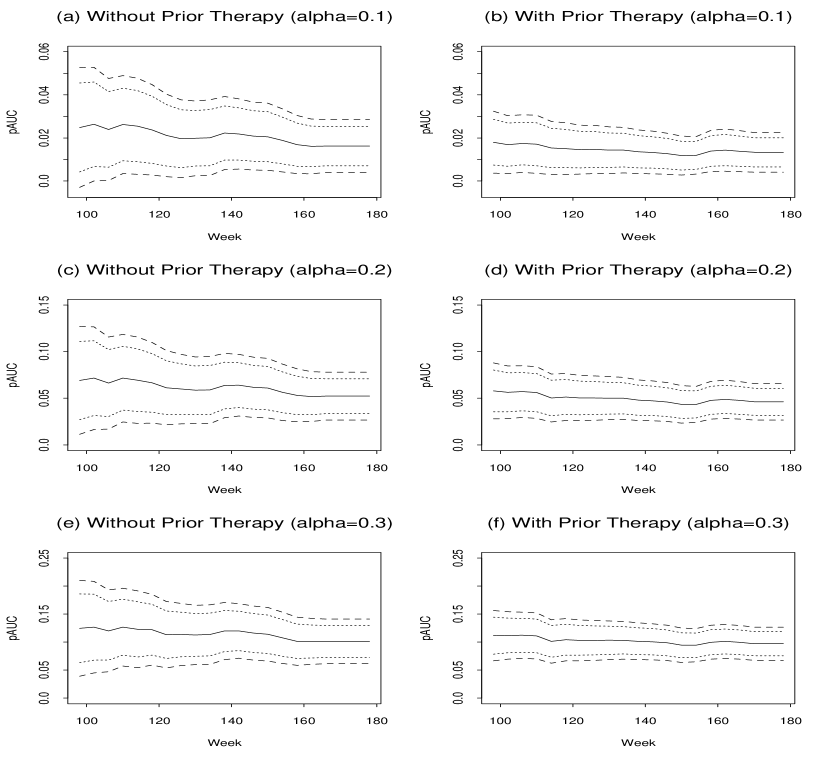
Figure 1: The estimated time-dependent pAUCs (solid curve) and the 0.95 pointwise confidence intervals (dotted curve) and simultaneous confidence bands (dashed curve).

To simplify the presentation, the marker and the time-dependent pAUC for non-therapy and therapy patients are denoted separately by $(Y^{(1)},\theta_{t}^{(1)}(q^{(1)}_{\alpha t}))$ and $(Y^{(2)},\theta_{t}^{(2)}(q^{(2)}_{\alpha t}))$. Based on two independent data sets $\{X^{(1)}_{i},\delta^{(1)}_{i},Y^{(1)}_{i}\}_{i=1}^{n_{1}}$ and $\{X^{(2)}_{i},\delta^{(2)}_{i},Y^{(2)}_{i}\}_{i=1}^{n_{2}}$, $\widehat{\theta}_{t}^{(1)}(\widehat{q}^{(1)}_{\alpha t})$ and $\widehat{\theta}_{t}^{(2)}(\widehat{q}^{(2)}_{\alpha t})$ are computed as $\widehat{\theta}_{t}(\widehat{q}_{\alpha t})$ in (2.3) using the bandwidths of 0.042 and 0.069, which are the minimizers of $ISE(\lambda)$ in (3.1). The confidence intervals for $\theta_{t}^{(k)}(q^{(k)}_{\alpha t})$’s are further constructed from (2.7) and (2.9). Due to the large variation of estimators before week 98, we only provide the estimated time-dependent pAUCs and 0.95 pointwise and simultaneous confidence bands from week 98 to the end of study in figures 1 (a)-(f). Based on the summary measures $\theta_{t}^{(k)}(q^{(k)}_{0.1t})$’s and compared with 0.005, one can conclude from the simultaneous confidence bands that the CD4 count is a useless biomarker in classifying patient’s survival time within the considered time period for both therapy and non-therapy patients. However, a different conclusion will be drawn at each time point based on the pointwise confidence intervals. The time-dependent pAUCs $\theta_{t}^{(1)}(q^{(1)}_{\alpha t})$ and $\theta_{t}^{(2)}(q^{(2)}_{\alpha t})$ are detected to be significantly higher than $0.5\alpha^{2}$ for $\alpha$=0.2 and 0.3 after week 110 and week 98, respectively. Figures 1 (a), (c), and (e) give a clear indication that the pAUCs decrease slightly over time for patients without prior therapy. However, the pAUCs stay very close to a constant throughout the study period for those with prior therapy (figures 1 (b), (d), and (f)).

The difference in the classification accuracies of $Y^{(1)}$ and $Y^{(2)}$ can be measured by the summary index $\gamma_{\alpha}(t)=\theta_{t}^{(1)}(q^{(1)}_{\alpha t})-\theta_{t}^{(2)}(q^{(2)}_{\alpha t})$. When $\alpha=1$, $\gamma_{\alpha}(t)$ is the usual comparison of AUCs in the time-dependent setting. It is natural to estimate $\gamma_{\alpha}(t)$ by $\widehat{\gamma}_{\alpha}(t)=\widehat{\theta}_{t}^{(1)}(\widehat{q}^{(1)}_{\alpha t})-\widehat{\theta}_{t}^{(2)}(\widehat{q}^{(2)}_{\alpha t})$. Along the same lines as the proof in the Appendix, we can derive that $\sqrt{n}(\widehat{\gamma}_{\alpha}(t)-\gamma_{\alpha}(t))$ converges weakly to a mean zero Gaussian process with variance-covariance function $\Gamma_{\alpha}(s,t)=\kappa^{-1}E[\Psi_{\alpha i}^{(1)}(s)\Psi_{\alpha i}^{(1)}(t)]+(1-\kappa)^{-1}E[\Psi_{\alpha i}^{(2)}(s)\Psi_{\alpha i}^{(2)}(t)]$ provided that $n_{1}/n\rightarrow\kappa$ ($0<\kappa<1$) as $n=(n_{1}+n_{2})\rightarrow\infty$, where $\Psi_{\alpha i}^{(k)}(t)$ is a counterpart of $\Psi_{\alpha i}(t)$, $k=1,2$. To make inference on $\gamma_{\alpha}(t)$, $\Gamma_{\alpha}(s,t)$ is first estimated by

$$\widehat{\Gamma}_{\alpha}(s,t)=\frac{n}{n_{1}^{2}}\sum_{i=1}^{n_{1}}\widehat{\Psi}_{\alpha i}^{(1)}(s)\widehat{\Psi}_{\alpha i}^{(1)}(t)+\frac{n}{n_{2}^{2}}\sum_{i=1}^{n_{2}}\widehat{\Psi}_{\alpha i}^{(2)}(s)\widehat{\Psi}_{\alpha i}^{(2)}(t).$$ (4.1)

A $(1-\varsigma)$ pointwise confidence interval for $\gamma_{\alpha}(t)$ and a $(1-\varsigma)$ simultaneous confidence band for $\{\gamma_{\alpha}(t):t\in[\tau_{1},\tau_{2}]\}$ are separately given via

$$\widehat{\gamma}_{\alpha}(t)\pm\frac{Z_{\varsigma/2}}{\sqrt{n}}\widehat{\Gamma}_{\alpha}^{\frac{1}{2}}(t,t)\text{ and }\{\widehat{\gamma}_{\alpha}(t)\pm\frac{L^{(\gamma)}_{\varsigma}}{\sqrt{n}}\widehat{\Gamma}_{\alpha}^{\frac{1}{2}}(t,t):t\in[\tau_{1},\tau_{2}]\}$$ (4.2)

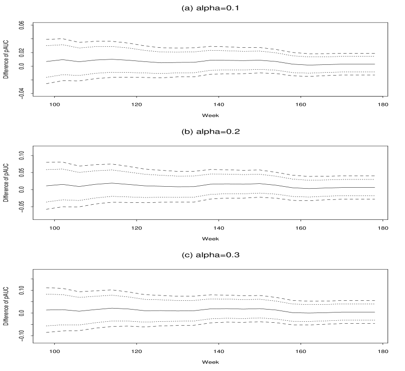
Figure 2: The estimated curves for the difference of the time-dependent pAUCs between non-therapy and therapy patients (solid curve) and the 0.95 pointwise confidence intervals (dotted curve) and simultaneous confidence bands (dashed curve).

with $L^{(\gamma)}_{\varsigma}$ being obtained as (2.8). It is revealed in figures 2 (a)-(c) that $\gamma_{\alpha}(t)$, $\alpha$=0.1, 0.2, and 0.3, tend to be positive within the study period and the difference becomes negligible as $\alpha$ increases. In other words, with small values of $FPR_{t}(y)$, a prior antiretroviral therapy might lower the discrimination ability of CD4 counts in classifying subject’s t-week survival. One possible explanation for this conclusion is that the prior therapy makes patients more homogeneous in survival time and CD4 counts. The estimates are further found to be around zero after about week 160. It means that for long term survival classification the performance of CD4 counts is irrelevant to whether patients receive prior therapy or not. Due to the large variability in the data, we could not detect any significant difference between $\theta_{t}^{(1)}(q^{(1)}_{\alpha t})$ and $\theta_{t}^{(2)}(q^{(2)}_{\alpha t})$. It would necessitate extremely large sample sizes to enable demonstration of significant differences between the pAUCs.

5 Discussion

For the time-dependent pAUC, it was traditionally estimated by the trapezoidal numerical integration method. The derivation for its sampling distribution becomes complicated and the computation load is prohibitively expensive. Although the inferences can be developed through a bootstrap technique, there is still no rigorous theoretical justification for this procedure. We can see in this article that the proposed estimators are simple and have explicit mathematical expressions. The confidence bands are built based on the asymptotic Gaussian process of the estimators as well as the corresponding estimates of the asymptotic variances. The estimation and inference procedures are further shown to be useful through simulation studies and an application to the ACTG 175 data.

It is detected from our numerical studies that the performance of the proposed estimator $\widehat{\theta}_{t}(\widehat{q}_{\alpha t})$ is very sensitive to small value of $\alpha$. To obtain a more stable estimate of $\theta_{t}(q_{\alpha t})$, a large sample size relative to $\alpha$ is usually suggested especially in the presence of censoring. Moreover, the price for the assumption of marker dependent censoring is to find an appropriate bandwidth in estimation. To this problem, we propose a simple and easily implemented selection procedure and show its good performance through simulations. As for the estimation of $\theta_{t}(q_{\alpha t})$, it can be also derived via using the bivariate estimation methods of Campbell (1981) or Burke (1988) for $S(t,y)$. However, these estimators are only valid under independent censorship which appears to be very limited and may not always be met in applications. One advantage of totally independent censoring assumption is that no smoothing technique is required.

In some empirical examples, censored survival data of the form $\{X_{i},\delta_{i},Y^{(1)}_{i},Y^{(2)}_{i}\}_{i=1}^{n}$ are often occurred in a paired design with $(Y^{(1)}_{i},Y^{(2)}_{i})$ being the different biomarkers of the $i$th subject. The scientific interest usually focuses on comparing the discrimination abilities of $Y^{(1)}$ and $Y^{(2)}$ on subject’s survival status at each time point within the study period. Obviously, the assumptions of marker dependent censoring made separately on $(T,C,Y^{(1)})$ and $(T,C,Y^{(2)})$ are often unreasonable in practice. Under a more flexible assumption of conditionally independent censorship ($T$ and $C$ are independent conditioning on $(Y^{(1)},Y^{(2)})$), the estimated joint survivor function of $T$ and $Y^{(1)}$ and that of $T$ and $Y^{(2)}$ in this article are quite inadequate in the estimation of $\gamma_{\alpha}(t)$ without modification. It is worthwhile to investigate the associated comparison procedure in our future study.

APPENDIX

For the proof of main results, the assumptions in Akritas (1994) and the conditions (A1: $f_{t}(y)=-\partial FPR_{t}(y)/\partial y$ exists with $\inf_{t}f_{t}(q_{\alpha t})>0$) and (A2: $\sup_{t}|\varsigma^{-1}\{FPR_{t}(q_{\alpha t}+\varsigma)-FPR_{t}(q_{\alpha t})\}+f_{t}(q_{\alpha t})|\rightarrow 0$ as $\varsigma\rightarrow 0$) are made throughout the rest of this paper.

Asymptotic Gaussian Process of $\widehat{\theta}_{t}(\widehat{q}_{\alpha t})$:

From Theorem 3.1 of Akritas (1994), one has

$$\sup_{t,y}|\sqrt{n}(\widehat{S}(t,y)-S(t,y))-\frac{\sqrt{n}}{n}\sum_{i=1}^{n}V_{i}(t,y)|=o_{p}(1),$$ (A.1)

where $V_{i}(t,y)=(S_{T}(t|Y_{i})+\xi_{i}(t))I(Y_{i}>y)-S(t,y)$ with $\xi_{i}(t)=-S_{T}(t|Y_{i})\int_{0}^{t}S_{X}^{-1}(u|Y_{i})$ $d_{u}M_{i}(u|Y_{i})$, $M_{i}(t|Y_{i})=I(X_{i}\leq t)\delta_{i}+\ln S_{T}(t\wedge X_{i}|Y_{i})$, and $t\wedge X_{i}=\min\{t,X_{i}\}$. Let $h_{ij}(t,y)=(1-S_{T}(t|Y_{i}))S_{T}(t|Y_{j})\phi_{ij}(y)$ and $H(t,y)=E[h_{ij}(t,y)]$. The uniform consistency of $\widehat{S}_{T}(t|y)$ (cf. Dabrowska (1987)) ensures that

$$\widehat{H}(t,y) = \frac{1}{n^{2}}\sum_{i\neq j}h_{ij}(t,y)+\frac{1}{n^{2}}\sum_{i\neq j}(S_{T}(t|Y_{i})-\widehat{S}_{T}(t|Y_{i}))S_{T}(t|Y_{j})\phi_{ij}(y)$$ (A.2)

$$+\frac{1}{n^{2}}\sum_{i\neq j}(1-S_{T}(t|Y_{i}))(\widehat{S}_{T}(t|Y_{j})-S_{T}(t|Y_{j}))\phi_{ij}(y)+r_{1n}(t,y)$$

with $\sup_{t,y}|r_{1n}(t,y)|=o_{p}(n^{-1/2})$. By a direct calculation and (A.1), a simplified form of the second term in the righthand side of (A.2) is obtained as follows:

$$\frac{1}{n}\sum_{j=1}^{n}S_{T}(t|Y_{j})I(Y_{j}>y)\{\frac{1}{n}\sum_{i=1}^{n}S_{T}(t|Y_{i})I(Y_{i}>Y_{j})-\widehat{S}(t,Y_{j})\}$$ (A.3)

$$= \frac{-1}{n^{2}}\sum_{i,j}S_{T}(t|Y_{j})\xi_{i}(t)\phi_{ij}(y)+r_{2n}(t,y),$$

where $\sup_{t,y}|r_{2n}(t,y)|=o_{p}(n^{-1/2})$. Similarly, the third term can be expressed as

$$\frac{1}{n^{2}}\sum_{i,j}(1-S_{T}(t|Y_{i}))\xi_{j}(t)\phi_{ij}(y)+r_{3n}(t,y)$$ (A.4)

with $\sup_{t,y}|r_{3n}(t,y)|=o_{p}(n^{-1/2})$. It follows from (A.2)-(A.4), the decomposition of a U-statistic into a sum of degenerate U-statistics (Serfling (1980)), and Corollary 4 of Sherman (1994) that

$$\sup_{t,y}|\sqrt{n}(\widehat{H}(t,y)-H(t,y))-\frac{\sqrt{n}}{n}\sum_{i=1}^{n}U_{i}(t,y)|=o_{p}(1),$$ (A.5)

where $U_{i}(t,y)=E[h_{ij}(t,y)+h_{ji}(t,y)|X_{i},Y_{i},\delta_{i}]-2H(t,y)+(S_{Y}(Y_{i})-S(t,y))\xi_{i}(t)I(Y_{i}>y)$. By the Taylor expansion of $\widehat{\theta}_{t}(y)=\widehat{H}(t,y)\{\widehat{S}_{T}(t)(1-\widehat{S}_{T}(t))\}^{-1}$ at $(\widehat{H}(t,y),\widehat{S}_{T}(t))=(H(t,y),S_{T}(t))$, (A.1), and (A.5), one has

$$\sup_{t,y}|\sqrt{n}(\widehat{\theta}_{t}(y)-\theta_{t}(y))-\frac{\sqrt{n}}{n}\sum_{i=1}^{n}\frac{U_{i}(t,y)+\eta(t,y)V_{i}(t,-\infty)}{S_{T}(t)(1-S_{T}(t))}|=o_{p}(1),$$ (A.6)

where $\eta(t,y)=H(t,y)(2S_{T}(t)-1)(S_{T}(t)-S_{T}^{2}(t))^{-1}$. Thus, $\sqrt{n}(\widehat{\theta}_{t}(q_{\alpha t})-\theta_{t}(q_{\alpha t}))$ can be shown to converge to a mean zero Gaussian process by an application of the functional cental limit theorem.

For the asymptotic Gaussian process of $\widehat{\theta}_{t}(\widehat{q}_{\alpha t})$, it is established through the equality $\sqrt{n}(\widehat{\theta}_{t}(\widehat{q}_{\alpha t})-\theta_{t}(q_{\alpha t}))=\sqrt{n}(\widehat{\theta}_{t}(\widehat{q}_{\alpha t})-\theta_{t}(\widehat{q}_{\alpha t}))+\sqrt{n}(\theta_{t}(\widehat{q}_{\alpha t})-\theta_{t}(q_{\alpha t}))$. Let $\sqrt{n}(\widehat{q}_{\alpha t}-q_{\alpha t})=\sqrt{n}(Q(\widehat{S})-Q(S))$ with $Q:S\rightarrow q_{\alpha t}$. By assumptions (A1)-(A2), the Hadamard differentiability of $Q$ is a direct result of Lemma A.1 in Daouia, Florens, and Simar (2008). Together with the functional delta method (cf. Van der Vaart (2000)), we have

$$\sup_{t}|\sqrt{n}(\widehat{q}_{\alpha t}-q_{\alpha t})-\frac{\sqrt{n}}{n}\sum_{i=1}^{n}\frac{V_{i}(t,q_{\alpha t})-\alpha V_{i}(t,-\infty)}{f_{t}(q_{\alpha t})S_{T}(t)}|=o_{p}(1).$$ (A.7)

and the weak convergence of $\sqrt{n}(\widehat{q}_{\alpha t}-q_{\alpha t})$. It is further ensured by (a version of) Lemma 19.24 of van der Vaart (2000) and (A.6) that

$$\sup_{t}|\sqrt{n}(\widehat{\theta}_{t}(\widehat{q}_{\alpha t})-\theta_{t}(\widehat{q}_{\alpha t})-\sqrt{n}(\widehat{\theta}_{t}(q_{\alpha t})-\theta_{t}(q_{\alpha t}))|=o_{p}(1).$$ (A.8)

Moreover, the first order Taylor expansion of $\theta_{t}(\widehat{q}_{\alpha t})$ at $\widehat{q}_{\alpha t}=q_{\alpha t}$, the continuity of $\partial\theta_{t}(y)/\partial y$, $\sup_{t}|\widehat{q}_{\alpha t}-q_{\alpha t}|=o_{p}(1)$, and the continuous mapping theorem imply that

$$\sup_{t}|\sqrt{n}(\theta_{t}(\widehat{q}_{\alpha t})-\theta_{t}(q_{\alpha t}))-\frac{\alpha S_{T}(t)-S_{Y}(q_{\alpha t})}{1-S_{T}(t)}f_{t}(q_{\alpha t})\sqrt{n}(\widehat{q}_{\alpha t}-q_{\alpha t})|=o_{p}(1).$$ (A.9)

It follows from (A.6)-(A.9) that

$$\sup_{t}|\sqrt{n}(\widehat{\theta}_{t}(\widehat{q}_{\alpha t})-\theta_{t}(q_{\alpha t}))-\frac{\sqrt{n}}{n}\sum_{i=1}^{n}\Psi_{\alpha i}(t)|=o_{p}(1),$$ (A.10)

$$\text{where }\Psi_{\alpha i}(t)=\frac{U_{i}(t,q_{\alpha t})+\eta(t,q_{\alpha t})V_{i}(t,-\infty)+(\alpha S_{T}(t)-S_{Y}(q_{\alpha t}))(V_{i}(t,q_{\alpha t})-\alpha V_{i}(t,-\infty))}{S_{T}(t)(1-S_{T}(t))}.$$

Finally, the proof is completed by applying the functional central limit theorem to the approximated term $n^{-1/2}\sum_{i=1}^{n}\Psi_{\alpha i}(t)$ in (A.10).

REFERENCES

Akritas, M. G. (1994). Nearest neighbor estimation of a bivariate distribution under random censoring. Annals of Statistics 22, 1299-1327.

Burke, M. D. (1988). Estimation of a bivariate distribution function under random censorship. Biometrika 75, 379-382.

Cai, T. and Dodd, L. E. (2008). Regression analysis for the partial area under the ROC curve. Statistica Sinica 18, 817-836.

Campbell, G. (1981). Nonparametric bivariate estimation with randomly censored data. Biometrika 68, 417-423.

Chambless, L. E. and Diao, G. (2006). Estimation of time-dependent area under the ROC curve for long-term risk prediction. Statistics in Medicine 25, 3474-3486.

Chiang, C. T., Wang, S. H., and Hung, H. (2008). Random weighting and Edgeworth expansion for the nonparametric time-dependent AUC estimator. Statistic Sinica. Accepted.

Chiang, C. T. and Hung, H. (2008). Nonparametric estimation for time-dependent AUC. Technical Report, National Taiwan University.

Dabrowska, D. M. (1987). Uniform consistency of nearest neighbor and kernel conditional Kaplan-Meier estimates. Technical Report No. 86, Univ. California, Berkeley.

Daouia, A., Florens, J. P., and Simar, L. (2008). Functional convergence of quantile-type frontiers with application to parametric approximations. Journal of Statistical Planning and Inference 138, 708-725.

Dodd, L. and Pepe, M. S. (2003). Partial AUC estimation and regression. Biometrics 59, 614-623.

Dwyer, A. J. (1996). In pursuit of a piece of the ROC. Radiology 201, 621-625.

Emir, B., Wieand, S., Jung, S. H., and Ying, Z. (2000). Comparison of diagnostic markers with repeated measurements: a non-parametric ROC curve approach. Statistics in Medicine 19, 511-523.

Hammer, S. M., Katzenstein, D. A., Hughes, M. D., Gundacker, H., Schooley, R. T., Haubrich, R. H., Henry, W. K., Lederman, M. M., Phair, J. P., Niu, M., Hirsch, M. S., and Merigan, T. C. (1996). A trial comparing nucleoside monotherapy with combination therapy in HIV-infected adults with CD4 cell counts from 200 to 500 per cubic millimeter. The New England Journal of Medicine 335, 1081-1090.

Heagerty, P. J., Lumley, T., and Pepe, M. S. (2000). Time-dependent ROC curves for censored survival data and a diagnostic marker. Biometrics 54, 124-135.

Jiang, Y., Metz, C. E., and Nishikawa, R. M. (1996). A receiver operating characteristic partial area index for highly sensitive diagnostic tests. Radiology 201, 745-750.

Lin, D. Y., Wei, L. J., Yang, I., and Ying, Z. (2000). Semiparametric regression for the mean and rate functions of recurrent events. Journal of the Royal Statistical Society B62, 711-730.

McClish, D. K. (1989). Analyzing a portion of the ROC curve. Medical Decision Making 9, 190-195.

Serfling, R. J. (1980). Approximation theorems of mathematical statistics. New York: Wiley.

Sherman, R. P. (1994). Maximal inequalities for degenerate U-processes with applications to optimization estimators. Annals of Statistics 22, 439-459.

van der Vaart, A. W. (2000). Asymptotic Statistics. Cambridge: Cambridge University Press.

Zhang, D. D., Zhou, X. H., Freeman, Daniel H. J., and Freeman, J. L. (2002). A non-parametric method for the comparison of partial areas under ROC curves and its application to large health care data set. Statistics in Medicine 21, 701-715.

Zhou, X. H., McClish, D. K., and Obuchowski, N. A. (2002). Statistical methods in diagnostic medicine. New York: Wiley.

Table 1

The averages $(Mean)$ and the standard deviations $(SD)$ of 500 estimates, the standard errors $(SE)$, and the empirical coverage probabilities $(CP)$

$c.r.=0\%$			$n=500$				$n=1000$
	Time	$\theta_{t}(q_{0.1t})$	Mean	SD	SE	CP	Mean	SD	SE	CP
	$t_{0.4}$	0.0264	0.0273	0.0044	0.0041	0.938	0.0269	0.0031	0.0029	0.944
$\widetilde{\theta}_{t}(\widetilde{q}_{0.1t})$	$t_{0.5}$	0.0269	0.0284	0.0045	0.0042	0.918	0.0275	0.0031	0.0030	0.934
	$t_{0.6}$	0.0279	0.0296	0.0046	0.0045	0.914	0.0288	0.0034	0.0031	0.926
	$t_{0.4}$	0.0264	0.0240	0.0043	0.0049	0.954	0.0247	0.0030	0.0034	0.948
$\widehat{\theta}_{t}(\widehat{q}_{0.1t})$	$t_{0.5}$	0.0269	0.0249	0.0042	0.0047	0.960	0.0256	0.0030	0.0032	0.938
$(\lambda_{opt})$	$t_{0.6}$	0.0279	0.0262	0.0046	0.0046	0.928	0.0269	0.0033	0.0033	0.942
$c.r.=30\%$			$n=500$				$n=1000$
$\lambda$	Time	$\theta_{t}(q_{0.1t})$	Mean	SD	SE	CP	Mean	SD	SE	CP
	$t_{0.4}$	0.0264	0.0268	0.0052	0.0040	0.834	0.0264	0.0034	0.0030	0.908
0.01	$t_{0.5}$	0.0269	0.0272	0.0055	0.0040	0.846	0.0272	0.0038	0.0030	0.874
	$t_{0.6}$	0.0279	0.0279	0.0055	0.0041	0.848	0.0280	0.0040	0.0031	0.882
	$t_{0.4}$	0.0264	0.0234	0.0050	0.0058	0.948	0.0243	0.0035	0.0041	0.950
$\lambda_{opt}$	$t_{0.5}$	0.0269	0.0248	0.0054	0.0056	0.932	0.0252	0.0037	0.0040	0.942
	$t_{0.6}$	0.0279	0.0264	0.0055	0.0056	0.924	0.0264	0.0039	0.0040	0.910
	$t_{0.4}$	0.0264	0.0190	0.0032	0.0062	0.894	0.0187	0.0021	0.0045	0.654
0.20	$t_{0.5}$	0.0269	0.0203	0.0037	0.0061	0.868	0.0200	0.0026	0.0044	0.698
	$t_{0.6}$	0.0279	0.0218	0.0045	0.0061	0.864	0.0218	0.0031	0.0045	0.762
$c.r.=50\%$			$n=500$				$n=1000$
$\lambda$	Time	$\theta_{t}(q_{0.1t})$	Mean	SD	SE	CP	Mean	SD	SE	CP
	$t_{0.4}$	0.0264	0.0266	0.0062	0.0042	0.786	0.0266	0.0043	0.0033	0.864
0.01	$t_{0.5}$	0.0269	0.0268	0.0064	0.0041	0.772	0.0270	0.0046	0.0033	0.828
	$t_{0.6}$	0.0279	0.0265	0.0066	0.0043	0.754	0.0275	0.0051	0.0034	0.792
	$t_{0.4}$	0.0264	0.0237	0.0057	0.0067	0.950	0.0243	0.0040	0.0047	0.960
$\lambda_{opt}$	$t_{0.5}$	0.0269	0.0250	0.0061	0.0064	0.918	0.0253	0.0045	0.0046	0.924
	$t_{0.6}$	0.0279	0.0266	0.0071	0.0064	0.892	0.0267	0.0049	0.0047	0.920
	$t_{0.4}$	0.0264	0.0192	0.0037	0.0073	0.952	0.0190	0.0025	0.0053	0.828
0.20	$t_{0.5}$	0.0269	0.0209	0.0047	0.0071	0.932	0.0203	0.0031	0.0052	0.846
	$t_{0.6}$	0.0279	0.0225	0.0056	0.0072	0.908	0.0221	0.0037	0.0055	0.864

Table 2

The averages $(Mean)$ and the standard deviations $(SD)$ of 500 estimates, the standard errors $(SE)$, and the empirical coverage probabilities $(CP)$

$c.r.=0\%$			$n=500$				$n=1000$
	Time	$\theta_{t}(q_{0.2t})$	Mean	SD	SE	CP	Mean	SD	SE	CP
	$t_{0.4}$	0.0770	0.0786	0.0086	0.0083	0.930	0.0780	0.0062	0.0058	0.922
$\widetilde{\theta}_{t}(\widetilde{q}_{0.2t})$	$t_{0.5}$	0.0776	0.0801	0.0084	0.0082	0.924	0.0785	0.0059	0.0058	0.932
	$t_{0.6}$	0.0794	0.0825	0.0086	0.0086	0.918	0.0808	0.0063	0.0060	0.920
	$t_{0.4}$	0.0770	0.0732	0.0085	0.0093	0.956	0.0745	0.0060	0.0064	0.950
$\widehat{\theta}_{t}(\widehat{q}_{0.2t})$	$t_{0.5}$	0.0776	0.0744	0.0081	0.0089	0.966	0.0755	0.0058	0.0061	0.952
$(\lambda_{opt})$	$t_{0.6}$	0.0794	0.0765	0.0088	0.0088	0.936	0.0777	0.0061	0.0062	0.948
$c.r.=30\%$			$n=500$				$n=1000$
$\lambda$	Time	$\theta_{t}(q_{0.2t})$	Mean	SD	SE	CP	Mean	SD	SE	CP
	$t_{0.4}$	0.0770	0.0774	0.0101	0.0080	0.850	0.0767	0.0067	0.0061	0.926
0.01	$t_{0.5}$	0.0776	0.0779	0.0101	0.0078	0.864	0.0780	0.0072	0.0060	0.884
	$t_{0.6}$	0.0794	0.0789	0.0100	0.0080	0.862	0.0797	0.0075	0.0061	0.874
	$t_{0.4}$	0.0770	0.0724	0.0102	0.0111	0.944	0.0742	0.0070	0.0077	0.962
$\lambda_{opt}$	$t_{0.5}$	0.0776	0.0744	0.0107	0.0106	0.926	0.0751	0.0071	0.0074	0.952
	$t_{0.6}$	0.0794	0.0771	0.0104	0.0106	0.938	0.0770	0.0074	0.0075	0.946
	$t_{0.4}$	0.0770	0.0648	0.0079	0.0125	0.932	0.0642	0.0053	0.0089	0.796
0.20	$t_{0.5}$	0.0776	0.0667	0.0086	0.0119	0.914	0.0663	0.0061	0.0085	0.808
	$t_{0.6}$	0.0794	0.0693	0.0095	0.0118	0.912	0.0694	0.0066	0.0086	0.854
$c.r.=50\%$			$n=500$				$n=1000$
$\lambda$	Time	$\theta_{t}(q_{0.2t})$	Mean	SD	SE	CP	Mean	SD	SE	CP
	$t_{0.4}$	0.0770	0.0770	0.0120	0.0084	0.820	0.0771	0.0083	0.0066	0.880
0.01	$t_{0.5}$	0.0776	0.0768	0.0122	0.0082	0.794	0.0775	0.0088	0.0065	0.846
	$t_{0.6}$	0.0794	0.0759	0.0127	0.0084	0.760	0.0785	0.0097	0.0066	0.814
	$t_{0.4}$	0.0770	0.0728	0.0118	0.0128	0.944	0.0740	0.0081	0.0089	0.966
$\lambda_{opt}$	$t_{0.5}$	0.0776	0.0748	0.0123	0.0122	0.926	0.0753	0.0086	0.0086	0.940
	$t_{0.6}$	0.0794	0.0774	0.0134	0.0122	0.902	0.0775	0.0090	0.0088	0.924
	$t_{0.4}$	0.0770	0.0654	0.0090	0.0146	0.966	0.0650	0.0064	0.0105	0.900
0.20	$t_{0.5}$	0.0776	0.0679	0.0105	0.0138	0.950	0.0670	0.0072	0.0101	0.906
	$t_{0.6}$	0.0794	0.0704	0.0115	0.0138	0.930	0.0700	0.0078	0.0102	0.908

Table 3

The averages $(Mean)$ and the standard deviations $(SD)$ of 500 estimates, the standard errors $(SE)$, and the empirical coverage probabilities $(CP)$

$c.r.=0\%$			$n=500$				$n=1000$
	Time	$\theta_{t}(q_{0.3t})$	Mean	SD	SE	CP	Mean	SD	SE	CP
	$t_{0.4}$	0.1420	0.1442	0.0120	0.0118	0.944	0.1433	0.0088	0.0083	0.940
$\widetilde{\theta}_{t}(\widetilde{q}_{0.3t})$	$t_{0.5}$	0.1423	0.1457	0.0115	0.0116	0.938	0.1434	0.0083	0.0082	0.936
	$t_{0.6}$	0.1446	0.1483	0.0120	0.0119	0.930	0.1461	0.0085	0.0084	0.938
	$t_{0.4}$	0.1420	0.1372	0.0121	0.0131	0.962	0.1388	0.0084	0.0090	0.952
$\widehat{\theta}_{t}(\widehat{q}_{0.3t})$	$t_{0.5}$	0.1423	0.1383	0.0117	0.0124	0.954	0.1396	0.0080	0.0086	0.958
$(\lambda_{opt})$	$t_{0.6}$	0.1446	0.1408	0.0123	0.0124	0.944	0.1424	0.0083	0.0086	0.962
$c.r.=30\%$			$n=500$				$n=1000$
$\lambda$	Time	$\theta_{t}(q_{0.3t})$	Mean	SD	SE	CP	Mean	SD	SE	CP
	$t_{0.4}$	0.1420	0.1424	0.0140	0.0116	0.880	0.1417	0.0095	0.0088	0.940
0.01	$t_{0.5}$	0.1423	0.1427	0.0142	0.0113	0.874	0.1430	0.0101	0.0085	0.882
	$t_{0.6}$	0.1446	0.1438	0.0137	0.0115	0.892	0.1451	0.0105	0.0086	0.874
	$t_{0.4}$	0.1420	0.1362	0.0144	0.0154	0.948	0.1387	0.0098	0.0106	0.962
$\lambda_{opt}$	$t_{0.5}$	0.1423	0.1383	0.0150	0.0147	0.932	0.1392	0.0099	0.0103	0.956
	$t_{0.6}$	0.1446	0.1414	0.0143	0.0146	0.940	0.1415	0.0102	0.0104	0.948
	$t_{0.4}$	0.1420	0.1265	0.0122	0.0174	0.938	0.1257	0.0082	0.0124	0.844
0.20	$t_{0.5}$	0.1423	0.1281	0.0129	0.0164	0.914	0.1276	0.0090	0.0118	0.836
	$t_{0.6}$	0.1446	0.1310	0.0137	0.0164	0.916	0.1313	0.0093	0.0118	0.874
$c.r.=50\%$			$n=500$				$n=1000$
$\lambda$	Time	$\theta_{t}(q_{0.3t})$	Mean	SD	SE	CP	Mean	SD	SE	CP
	$t_{0.4}$	0.1420	0.1417	0.0167	0.0122	0.826	0.1419	0.0116	0.0095	0.892
0.01	$t_{0.5}$	0.1423	0.1407	0.0168	0.0118	0.824	0.1420	0.0120	0.0093	0.866
	$t_{0.6}$	0.1446	0.1389	0.0176	0.0120	0.796	0.1432	0.0133	0.0095	0.826
	$t_{0.4}$	0.1420	0.1369	0.0168	0.0176	0.948	0.1383	0.0115	0.0122	0.964
$\lambda_{opt}$	$t_{0.5}$	0.1423	0.1390	0.0173	0.0168	0.934	0.1394	0.0119	0.0119	0.948
	$t_{0.6}$	0.1446	0.1418	0.0184	0.0169	0.928	0.1421	0.0122	0.0121	0.948
	$t_{0.4}$	0.1420	0.1273	0.0137	0.0201	0.968	0.1267	0.0098	0.0144	0.910
0.20	$t_{0.5}$	0.1423	0.1295	0.0154	0.0190	0.954	0.1285	0.0105	0.0138	0.910
	$t_{0.6}$	0.1446	0.1321	0.0163	0.0190	0.938	0.1318	0.0113	0.0139	0.904

Table 4

The empirical coverage probabilities of $0.95$ simultaneous confidence bands

$c.r.=0\%$		$n=500$		$n=1000$
	$\alpha$	$[t_{0.4},t_{0.5}]$	$[t_{0.4},t_{0.6}]$	$[t_{0.4},t_{0.5}]$	$[t_{0.4},t_{0.6}]$
	0.1	0.904	0.892	0.932	0.928
$\widetilde{\theta}_{t}(\widetilde{q}_{\alpha t})$	0.2	0.922	0.908	0.932	0.934
	0.3	0.930	0.908	0.940	0.942
	0.1	0.962	0.942	0.936	0.932
$\widehat{\theta}_{t}(\widehat{q}_{\alpha t})$	0.2	0.968	0.952	0.948	0.944
$\lambda_{opt}$	0.3	0.958	0.950	0.946	0.952
$c.r.=30\%$		$n=500$		$n=1000$
$\lambda$	$\alpha$	$[t_{0.4},t_{0.5}]$	$[t_{0.4},t_{0.6}]$	$[t_{0.4},t_{0.5}]$	$[t_{0.4},t_{0.6}]$
	0.1	0.800	0.754	0.854	0.824
0.01	0.2	0.838	0.802	0.890	0.862
	0.3	0.860	0.838	0.892	0.856
	0.1	0.936	0.920	0.948	0.924
$\lambda_{opt}$	0.2	0.942	0.928	0.952	0.948
	0.3	0.938	0.938	0.952	0.952
	0.1	0.888	0.878	0.708	0.732
0.20	0.2	0.920	0.924	0.830	0.856
	0.3	0.934	0.936	0.846	0.876
$c.r.=50\%$		$n=500$		$n=1000$
$\lambda$	$\alpha$	$[t_{0.4},t_{0.5}]$	$[t_{0.4},t_{0.6}]$	$[t_{0.4},t_{0.5}]$	$[t_{0.4},t_{0.6}]$
	0.1	0.702	0.614	0.778	0.726
0.01	0.2	0.750	0.688	0.808	0.756
	0.3	0.774	0.720	0.830	0.798
	0.1	0.924	0.886	0.954	0.926
$\lambda_{opt}$	0.2	0.936	0.898	0.954	0.936
	0.3	0.948	0.914	0.946	0.942
	0.1	0.940	0.896	0.868	0.860
0.20	0.2	0.966	0.948	0.918	0.908
	0.3	0.966	0.952	0.918	0.918