Kondo Effect of a Magnetic Ion Vibrating in a Harmonic Potential

Abstract

To discuss Kondo effects of a magnetic ion vibrating in the sea of conduction electrons, a generalized Anderson model is derived. The model includes a new channel of hybridization associated with phonon emission or absorption. In the simplest case of the localized electron orbital with the $s$-wave symmetry, hybridization with $p$-waves becomes possible. Interesting interplay among the conventional $s$-wave Kondo effect and the $p$-wave one and the Yu-Anderson type Kondo effect is found and the ground state phase diagram is determined by using the numerical renormalization group method. Two different types of stable fixed points are identified and the two-channel Kondo fixed points are generically realized on the boundary.

1 Introduction

Recently, a new type of ionic structure, a network of cages filled or unfilled by guest ions, has attracted much interest in the research area of condensed matter physics. When the radius of filled ion is smaller than the size of cage, the guest ions vibrate with large amplitude but almost without effect of interference with oscillations of the ions in the neighboring cages. It is expected that various unusual phenomena are possible due to such incoherent vibrations. Typical examples of this class of materials are $\beta$-pyrochlore oxides AOs₂O₆(A $=$ K, Rb or Cs), filled skutterudites RT₄X${}_{12}($R $=$ rare earth or alkaline earth; T $=$ Fe, Ru, Pt or Os; X $=$ P, As, Ge or Sb$)$ and type-I clathrate compounds.

The family of $\beta$-pyrochlore oxides, especially KOs₂O₆, is a good example where several qualitatively new phenomena are observed due to the anharmonicity of the cage potential[1]: concave-downward temperature dependence of resistivity[2], peak structure of NMR relaxation rate at potassium site at low temperatures[3], occurrence of superconductivity[4] and the structural phase transition which takes place below the superconducting transition temperature[2]. Concerning the resistivity and the NMR relaxation rate, Dahm and one of the authors considered a simple model for the anharmonic potential which includes the fourth order term of the ion displacement. They have shown that the unusual temperature dependence of these quantities are explained by calculating the retarded phonon propagator within the self-consistent quasi-harmonic approximation[5]. Detailed properties of the spectral function of the local ion are also investigated for various types of the cage potential including a double-well type[6]. The more realistic model that the ion vibrates in the three-dimensional cage potential with the third order anharmonic term specific to the tetrahedral symmetry of the $\beta$-pyrochlore compounds is discussed by one of the authors and Tsunetsugu[7, 8, 9]. It is shown that the third order anharmonic term has important effect on the superconductivity and is also responsible to the first order structural transition below the superconducting transition temperature.

Another interesting behavior is reported for the filled skutterudite compound, SmOs₄Sb₁₂[10, 11, 12, 13, 14]. It shows a large specific heat coefficient $\gamma$, which is robust against magnetic fields[11]. One possible scenario of this behavior is that a non-magnetic Kondo effect is realized by local vibrations of the guest ions[15, 16]. Motivated by the unusual heavy fermion behaviors of SmOs₄Sb₁₂, we have started a systematic study on the interplay between local electron correlation and electron-phonon coupling[17].

Let us review the previous studies related to Kondo effect coupled with local vibrations. To include effects of the local oscillations, two different types of models have been considered, the breathing mode of the cage and the transverse modes of the cage, i.e., the relative displacement between the ion and the cage.

Firstly, a theoretical model of a magnetic ion coupled with the breathing mode is known as Anderson-Holstein model[18]. In this model the one-electron energy level of the impurity orbital is modified by the amplitude of the breathing mode. By applying Lang-Firsov transformation[19], it can be shown that the interaction induces an effectively attractive electron-electron interaction (for example see Ref. References). If the electron-phonon coupling overcomes Coulomb repulsion, the electronic states of the impurity result in a quasi degenerate doublet, the empty and the doubly occupied states. If there is a matrix element between the doublet, it is possible that the non-magnetic doublet works as a pseudo spin and induces Kondo effect. Actually, a recent study shows that magnetically robust Kondo effect is possible even in relatively high magnetic fields when the effect of anharmonicity of the breathing mode is included[21].

Secondly, a model of a non-magnetic ion which oscillates in the sea of conduction electrons was proposed by Yu and Anderson[22]. In this model, the conduction electrons are scattered by the vibrations of the ion. For simplicity spins of conduction electrons are neglected. Yu and Anderson considered only the first order term of ionic displacement which produced the scattering processes between the $s$-wave conduction electrons to the $p$-wave ones. It is shown that the resultant effective potential for the ion displacement behaves like a double well potential when the electron-phonon coupling is strong. Therefore a new type of Kondo effect is expected because logarithmic divergence appears when there are doubly degenerate states connected each other through scattering processes of conduction electrons[23, 24, 25].

This paper is a comprehensive report on the effects of vibration of a magnetic ion coupled with spinful conduction electrons. Some of the results have been published in the previous letter[17]. In §2 we construct a generalized impurity Anderson model of the magnetic ion. When we ignore spin-orbit interaction, the generalized gradient theorem[26] enables us to expand hybridization term with respect to the ion displacement. As a result phonon-assisted hybridization is naturally induced in addition to the conventional one. In §3 and §4, we apply the numerical renormalization group (NRG) method[27, 28] to the simplest case, where the impurity ion with an $s$-wave orbital vibrates in a one-dimensional harmonic potential. From the analysis of energy spectra obtained from the NRG calculations, one can identify three different types of NRG flows at low temperatures which define the low energy fixed points. We obtain the phase diagram characterized by the fixed points in the parameter space of phonon-assisted hybridization and Coulomb interaction. The fixed point analysis is described in detail in the present paper. Various physical quantities which include the spin and charge susceptibilities and the mean square amplitude of the displacement are also discussed. Finally, conclusions and some future problems are summarized in §5.

2 A generalized impurity Anderson model for a vibrating magnetic ion

2.1 Expansion of hybridization term by ion displacement

In this section we derive a generalized impurity Anderson model for a magnetic ion vibrating in a cage potential. When the ion is static, it has to be equivalent to the usual impurity Anderson model[29]. It is assumed that the effects of vibrations are taken into account through hybridization modified by the shift of the ionic position. Conduction electrons are assumed to be a non-interacting system and decomposed into the partial waves,

$$\mathit{H}_{\text{c}} =\sum_{\bm{k}\sigma}\varepsilon(\bm{k})c^{\dagger}_{\bm{k}\sigma}c_{\bm{k}\sigma}$$

$$=\sum_{k\sigma}\sum_{\ell m}\varepsilon(k)c^{\dagger}_{\ell m\sigma}(k)c_{\ell m\sigma}(k),$$ (2.1)

where $\varepsilon(\bm{k})$ is the dispersion relation and $c_{\bm{k}\sigma}$ $(c^{\dagger}_{\bm{k}\sigma})$ is an annihilation (creation) operator of the conduction electrons. $c_{\ell m\sigma}(k)$ $(c^{\dagger}_{\ell m\sigma}(k))$ is defined from $c_{\bm{k}\sigma}$ $(c^{\dagger}_{\bm{k}\sigma})$ by using the spherical harmonics $Y_{\ell m}(\hat{\bm{k}})$,

$$c_{\ell m\sigma}(k)=\sqrt{4\pi}\sum_{\hat{\bm{k}}}Y^{*}_{\ell m}(\hat{\bm{k}})c_{\bm{k}\sigma}.$$ (2.2)

The dynamics of the ion with position vector $\bm{Q}$ is described by the following Hamiltonian,

$$\mathit{H}_{\text{ion}} =-\frac{\hbar^{2}}{2M}(\nabla_{\bm{Q}})^{2}+V_{\text{cage}}(\bm{Q}),$$ (2.3)

where $V_{\text{cage}}(\bm{Q})$ is the cage potential and $M$ the mass of the ion. Hybridization modified by the ion displacement $\bm{Q}$ is expressed by the overlap integral between a plane wave $(1/\sqrt{\Omega})\text{e}^{\text{i}\bm{k}\cdot\bm{r}}$ and the localized orbitals of the magnetic ion, where $\Omega$ is the volume of the system. Without the spin orbit interaction, $\ell$-wave electron orbitals, $\psi_{\ell m}(\bm{r})\equiv u_{\ell}(r)Y_{\ell m}(\hat{\bm{r}})$, satisfy the following $\mathrm{Schr\ddot{o}dinger}$ equation,

$$\biggl{(}-\frac{\hbar^{2}\nabla^{2}}{2m}+V_{\text{nucleus}}(r)-\varepsilon_{\ell}\biggr{)}\psi_{\ell m}(\bm{r})=0,$$ (2.4)

where the potential $V_{\text{nucleus}}(r)$ is assumed to be isotropic and $m$ is the mass of electron. When the ion is shifted from the origin by $\bm{Q}$, the relative coordinate from the ion to electron coordinate $\bm{r}$ is given by $\bm{r}-\bm{Q}$. Therefore the overlap integrals are expressed by

$$V_{(\bm{k};\ell m)}(\bm{Q})=\frac{g}{\sqrt{\Omega}}\int d^{3}\bm{r}e^{-\text{i}\bm{k}\cdot\bm{r}}\psi_{\ell m}(\bm{r}-\bm{Q}),$$ (2.5)

where $g$ is a coupling constant. With these integrals, hybridization terms modified by the ion displacement are given as

$$\mathit{H}_{\text{hyb}}=\sum_{\bm{k}\sigma}\sum_{m}\bigl{[}V_{(\bm{k};\ell m)}(\bm{Q})c^{\dagger}_{\bm{k}\sigma}f_{\ell m\sigma}+\text{h.c.}\bigr{]},$$ (2.6)

where $f_{\ell m\sigma}$ $(f^{\dagger}_{\ell m\sigma})$ are the annihilation (creation) operators for the localized $\ell$-wave orbitals. We expand the overlap integrals with respect to the ion displacement $\bm{Q}$. In this paper we focus on the first order terms of $\bm{Q}$. The hybridization terms expanded within $O(\bm{Q})$ are given as

$$\mathit{H}_{\text{hyb}}= \sum_{km\sigma}\biggl{\{}V_{\ell}c^{\dagger}_{\ell m\sigma}(k)f_{\ell m\sigma}+\sum^{1}_{m^{\prime}=-1}q^{*}_{1,m^{\prime}}$$

$$\times \ \biggl{[}V^{(m,m^{\prime})}_{\ell+1}c^{\dagger}_{\ell+1,m+m^{\prime}\sigma}(k)f_{\ell m\sigma}$$

$$+V^{(m,m^{\prime})}_{\ell-1}c^{\dagger}_{\ell-1,m+m^{\prime}\sigma}(k)f_{\ell m\sigma}\biggr{]}+\text{h.c.}\biggr{\}},$$ (2.7)

where $V_{\ell}$, $V^{(m,m^{\prime})}_{\ell\pm 1}$ and $q_{1,m}$ are defined in Appendix. It is obvious that the rotational symmetry $SO(3)$ is preserved in the generalized hybridization term (2.7).

Under the simplest assumption that the ion has an $s$-wave electron orbital, the hybridization terms (2.7) are rewritten based on the Cartesian coordinate system as

$$\mathit{H}_{\text{hyb}}= \ \ \ \sum_{k\sigma}\bigl{\{}V_{0}c^{\dagger}_{0\sigma}(k)f_{\sigma}+\text{h.c.}\bigr{\}}$$

$$+\sum_{k\sigma}\sum_{i=x,y,z}\bigl{\{}\overline{V_{1}}c^{\dagger}_{1,i\sigma}(k)f_{\sigma}q_{i}+\text{h.c.}\bigr{\}},$$ (2.8)

where $c_{0\sigma}$ $(c_{1,i\sigma})$ are the annihilation operators for the $s$ $(p_{i})$-wave components of the conduction electrons. It is verified easily that $V^{(0,0)}_{1}=V^{(0,\pm 1)}_{1}\equiv\overline{V_{1}}$ because of the rotational invariance.

For simplicity, we study the situation that the ion vibrates along one direction, say $x$-direction. Using a one-dimensional harmonic potential $(1/2)M\omega^{2}Q^{2}$, we get the Hamiltonian for this study,

$$\mathit{H}= \mathit{H}_{\text{c}}+\mathit{H}_{\text{hyb}}+\mathit{H}_{\text{local}},$$ (2.9)

$$\mathit{H}_{\text{c}}= \sum_{k\sigma}\varepsilon(k)\bigl{\{}c^{\dagger}_{0\sigma}(k)c_{0\sigma}(k)+c^{\dagger}_{1\sigma}(k)c_{1\sigma}(k)\bigr{\}},$$ (2.10)

$$\mathit{H}_{\text{hyb}}= \sum_{k\sigma}\bigl{\{}V_{0}c^{\dagger}_{0\sigma}(k)f_{\sigma}+\text{h.c.}$$

$$+V_{1}c^{\dagger}_{1\sigma}(k)f_{\sigma}(a+a^{\dagger})+\text{h.c.}\bigr{\}},$$ (2.11)

$$\mathit{H}_{\text{local}}= \hbar\omega a^{\dagger}a+\varepsilon_{f}\sum_{\sigma}f^{\dagger}_{\sigma}f_{\sigma}+Uf^{\dagger}_{\uparrow}f_{\uparrow}f^{\dagger}_{\downarrow}f_{\downarrow},$$ (2.12)

where $\overline{V_{1}}/\sqrt{2}$ is set to $V_{1}$ and $a$ $(a^{\dagger})$ is the annihilation (creation) operator of the phonon. For the localized electron orbital, the annihilation (creation) operator is expressed by $f_{\sigma}$ $(f^{\dagger}_{\sigma})$ and $\epsilon_{f}$ is its energy given by eq. (2.4) and $U$ the Coulomb interaction. When we restrict the isotropic degrees of freedom of the ionic vibrations to one particular direction, the $SO(3)$ symmetry is lowered to the discrete inversion symmetry; $r\rightarrow-r$ and $Q\rightarrow-Q$.

2.2 Comments on the symmetries

There are three relevant quantum numbers for the present model (2.9)$-$(2.12). It is obvious that the total electron number $N^{\text{tot}}$ and the $z$ component of total spin $S^{\text{tot}}_{z}$ are conserved. The last one is related to the inversion symmetry mentioned in the previous subsection. The operation of the inversion $\mathcal{P}$ is described in the second-quantized notations,

$$\mathcal{P}f_{\sigma}\mathcal{P}^{-1} =f_{\sigma},$$ (2.13)

$$\mathcal{P}c_{0\sigma}(k)\mathcal{P}^{-1} =c_{0\sigma}(k),$$ (2.14)

$$\mathcal{P}c_{1\sigma}(k)\mathcal{P}^{-1} =-c_{1\sigma}(k),$$ (2.15)

$$\mathcal{P}q\mathcal{P}^{-1} =-q.$$ (2.16)

We characterize the inversion symmetry by the total parity $P$ which is defined by the sum between the number of $p$-channel conduction electrons $N_{p}$ and the number of harmonic phonons $N_{\text{ph}}$, namely $P=N_{p}+N_{\text{ph}}\equiv 0$ or $1$ $(\text{mod}\ 2)$[30]. This is based on the fact that, within $O(\bm{Q})$, phonon-assisted hopping between the impurity orbital and the $p$-channel conduction electrons has to accompany absorption or emission of one phonon. This quantum number plays a crucial role in the analyses of the energy spectra.

In the original model used by Yu and Anderson (YA model)[22], it is assumed that a non-magnetic ion, which is trapped in a one-dimensional harmonic potential, vibrates in spinless conduction electrons. The first order process of the displacement induces scattering processes between the $s$-wave and $p$-wave conduction electrons. No localized electron orbital is introduced in the model. The original YA model is written as

$$\mathit{H}_{\text{YA}}= \ \ \ \sum_{k}\bigl{\{}\varepsilon_{0}(k)c^{\dagger}_{0}(k)c_{0}(k)+\varepsilon_{1}(k)c^{\dagger}_{1}(k)c_{1}(k)\bigr{\}}$$

$$+\sum_{k,k^{\prime}}\bigl{\{}V_{1}c^{\dagger}_{0}(k)c_{1}(k^{\prime})(a+a^{\dagger})+\text{h.c.}\bigr{\}}$$

$$+\hbar\omega a^{\dagger}a,$$ (2.17)

where $c_{0}(k)$ $(c_{1}(k))$ are the annihilation operators for the spinless $s$-wave $(p$-wave$)$ conduction electrons with the dispersion relation $\varepsilon_{0}(k)$ $(\varepsilon_{1}(k))$.

In general, $\varepsilon_{0}(k)$ and $\varepsilon_{1}(k)$ are different. However if we assume that $\varepsilon_{0}(k)$ and $\varepsilon_{1}(k)$ are the same, an artificial symmetry comes into existence. The symmetry, which we call channel symmetry, is the invariance under the following transformation $\mathcal{I}$,

$$\mathcal{I}c_{0}(k)\mathcal{I}^{-1} =c_{1}(k),$$ (2.18)

$$\mathcal{I}c_{1}(k)\mathcal{I}^{-1} =c_{0}(k).$$ (2.19)

With the channel symmetry, the Hamiltonian (2.17) can be decomposed into two detached parts by introducing the bonding and antibonding orbitals,

$$c_{\text{e}}(k)=\frac{c_{0}(k)+c_{1}(k)}{\sqrt{2}},$$ (2.20)

$$c_{\text{o}}(k)=\frac{c_{0}(k)-c_{1}(k)}{\sqrt{2}},$$ (2.21)

and there is no matrix element between the two potential minima in contrast to the implicit assumption made by Yu and Anderson. Therefore the breaking of the channel symmetry is needed for the realization of Yu and Anderson type Kondo (YAK) effect. Matsuura and Miyake showed that potential scattering processes of the second order of the ion displacement play such a role[31].

These discussions are also valid for the spinful fermion case. As for the present Hamiltonian (2.9), the introduction of the localized impurity orbital serves as a source of breaking of the channel symmetry. Therefore the Hamiltonian (2.9) at $U=0$ is one realization of the YA model extended to the spinful case.

3 Numerical renormalization group approach

3.1 Mapping to Wilson chains

It is well known that for the ordinary impurity Anderson model the numerical renormalization group (NRG) method is a powerful one to calculate energy spectra and various physical quantities with high accuracy[27, 28]. We apply the NRG method to the present model by discretizing the two continuous conduction bands in the logarithmic energy scales characterized by $\varLambda$. Both the $s$-wave and $p$-wave conduction bands can be discretized in the same way because the dispersion relation $\varepsilon(\bm{k})$ is assumed to have no angular dependence on $\bm{k}$. The discretized Hamiltonian is given by the two one-dimensional half-chains corresponding to the $s$-wave and $p$-wave conduction bands, which may be called Wilson chains,

$$\mathit{H_{N}}=\varLambda^{\frac{N-1}{2}}$$

$$\times \Biggl{\{}\ \sum^{N-1}_{n=0,\sigma}\varLambda^{-\frac{n}{2}}\xi_{n}\bigl{[}s^{\dagger}_{n,\sigma}s_{n+1,\sigma}+p^{\dagger}_{n,\sigma}p_{n+1,\sigma}+\text{h.c.}\bigr{]}$$

$$\ +\sum_{\sigma}\bigl{[}\widetilde{V_{0}}s^{\dagger}_{0,\sigma}f_{\sigma}+\widetilde{V_{1}}p^{\dagger}_{0,\sigma}f_{\sigma}(a+a^{\dagger})+\text{h.c.}\bigr{]}$$

$$\ +\frac{\widetilde{U}}{2}\biggl{(}\sum_{\sigma}f^{\dagger}_{\sigma}f_{\sigma}-1\biggr{)}^{2}+\biggl{(}\widetilde{\varepsilon_{f}}+\frac{\widetilde{U}}{2}\biggr{)}\sum_{\sigma}f^{\dagger}_{\sigma}f_{\sigma}$$

$$\ +\hbar\widetilde{\omega}a^{\dagger}a\Biggr{\}}.$$ (3.1)

Here, for a constant density of states $\rho=1/2D$ with the band width of $2D$ the $n$-th hopping matrix element $\xi_{n}$ is given by

$$\xi_{n}=\frac{1-\varLambda^{-n-1}}{\sqrt{1-\varLambda^{-2n-1}}\sqrt{1-\varLambda^{-2n-3}}}.$$ (3.2)

All the parameters with tilde are multiplied by the constant factor $2/\{D(1+\varLambda^{-1})\}$. From now on we treat the symmetric case, $2\varepsilon_{f}+U=0$, for simplicity. The Hamiltonian (3.1) is block-diagonalized and each block is characterized by the set of quantum numbers, $N^{\text{tot}}$, $S^{\text{tot}}_{z}$ and the parity $P$ as discussed above. We set various parameters for NRG calculations as follows; $\varLambda=3.0$, cutoff number of phonon excitations 50, band width $D=1.0$ and $M=15000$ states are kept at each NRG step.

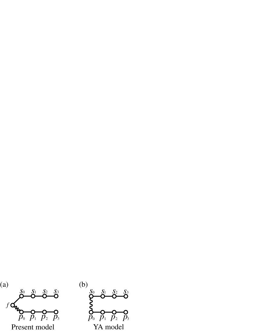
Figure 1: (Color online) (a) Graphical representation of the Hamiltonian (3.1). The wavy line represents phonon-assisted hopping while the straight lines usual hoppings. (b) The YA model mapped to the Wilson chains.

A graphical representation of the Hamiltonian (3.1) is shown in Fig. 1(a). For comparison, the YA model mapped to the Wilson chains is also shown in Fig. 1(b). From these pictures, we understand that within the first order of ion displacement there is the channel symmetry in the original YA model unlike the present model when the same hopping matrix elements are used for both channels.

3.2 Two-site problem

To investigate the effect of multi-phonon excitations, we consider the two-site Hamiltonian consisting of $f$ and $p_{0}$ sites in the Hamiltonian (3.1),

$$\mathit{H}_{\text{2-site}}= \mathit{H}^{(0)}_{\text{2-site}}+\mathit{H}^{(1)}_{\text{2-site}},$$ (3.3)

$$\mathit{H}^{(0)}_{\text{2-site}}= V_{1}\sum_{\sigma}\bigl{\{}p^{\dagger}_{0,\sigma}f_{\sigma}+\text{h.c.}\bigr{\}}(a+a^{\dagger})$$

$$+\hbar\omega a^{\dagger}a,$$ (3.4)

$$\mathit{H}^{(1)}_{\text{2-site}}= \frac{U}{2}\biggl{(}\sum_{\sigma}f^{\dagger}_{\sigma}f_{\sigma}-1\biggr{)}^{2}.$$ (3.5)

For $U=0$, the two-site Hamiltonian is solved exactly by using the canonical transformation called Lang-Firsov transformation[19], $e^{\text{i}S}$ with

$$S=\text{i}\lambda\sum_{\sigma}(-A^{\dagger}_{\sigma}A_{\sigma}+B^{\dagger}_{\sigma}B_{\sigma})(a-a^{\dagger}),$$ (3.6)

where $A_{\sigma}$ and $B_{\sigma}$ are the annihilation operator for the antibonding and bonding orbitals, $A_{\sigma}=(1/\sqrt{2})(f_{\sigma}-p_{0,\sigma})$ and $B_{\sigma}=(1/\sqrt{2})(f_{\sigma}+p_{0,\sigma})$. The coupling constant is given by $\lambda\equiv-V_{1}/\hbar\omega$. Then the transformed Hamiltonian is written as

$$\text{e}^{-\text{i}S}\mathit{H}^{(0)}_{\text{2-site}}\text{e}^{\text{i}S}$$

$$= -\frac{V^{2}_{1}}{\hbar\omega}\biggl{\{}\sum_{\sigma}(-A^{\dagger}_{\sigma}A_{\sigma}+B^{\dagger}_{\sigma}B_{\sigma})\biggr{\}}^{2}+\hbar\omega a^{\dagger}a.$$ (3.7)

We obtain the doubly degenerate ground states $|\text{L}\bigl{>}$ and $|\text{R}\bigl{>}$, which may be called polaron doublet (PD), with the ground-state energy $E_{\text{PD}}$,

$$|\text{L}\bigl{>}= B^{\dagger}_{\uparrow}B^{\dagger}_{\downarrow}|\text{vac}\bigl{>}_{\text{el}}|\ell\bigl{>}_{\text{ph}}$$

$$\ \ \ \ \ \text{with}\ |\ell\bigl{>}_{\text{ph}}=\text{e}^{-2\lambda(a-a^{\dagger})}|0\bigl{>}_{\text{ph}},$$ (3.8)

$$|\text{R}\bigl{>}= A^{\dagger}_{\uparrow}A^{\dagger}_{\downarrow}|\text{vac}\bigl{>}_{\text{el}}|r\bigl{>}_{\text{ph}}$$

$$\ \ \ \ \ \text{with}\ |r\bigl{>}_{\text{ph}}=\text{e}^{2\lambda(a-a^{\dagger})}|0\bigl{>}_{\text{ph}},$$ (3.9)

$$E_{\text{PD}}= -\frac{4V^{2}_{1}}{\hbar\omega}.$$ (3.10)

These two degenerate states are characterized by the expectation values of the ionic position $q$,

$$\bigl{<}\text{L}|q|\text{L}\bigl{>}=-\bigl{<}\text{R}|q|\text{R}\bigl{>}=2\sqrt{2}\lambda,$$ (3.11)

$$\bigl{<}\text{L}|q^{2}|\text{L}\bigl{>}=\bigl{<}\text{R}|q^{2}|\text{R}\bigl{>}=\frac{16\lambda^{2}+1}{2}.$$ (3.12)

One can see that the PD is formed both for spinful and spinless cases and it plays a similar role as the localized spin for the usual spin Kondo effect.

In the following discussion, it is important to note that the electron parts of the doublet are written as

$$B^{\dagger}_{\uparrow}B^{\dagger}_{\downarrow}|\text{vac}\bigl{>}_{\text{el}}= |\text{LS}\bigl{>}_{\text{el}}+|\text{PS}\bigl{>}_{\text{el}},$$ (3.13)

$$A^{\dagger}_{\uparrow}A^{\dagger}_{\downarrow}|\text{vac}\bigl{>}_{\text{el}}= |\text{LS}\bigl{>}_{\text{el}}-|\text{PS}\bigl{>}_{\text{el}},$$ (3.14)

where

$$|\text{LS}\bigl{>}_{\text{el}} \equiv\frac{f^{\dagger}_{\uparrow}f^{\dagger}_{\downarrow}+p^{\dagger}_{0,\uparrow}p^{\dagger}_{0,\downarrow}}{2}|\text{vac}\bigl{>}_{\text{el}}$$ (3.15)

represents a local singlet with even parity while

$$|\text{PS}\bigl{>}_{\text{el}} \equiv\frac{f^{\dagger}_{\uparrow}p^{\dagger}_{0,\downarrow}-f^{\dagger}_{\downarrow}p^{\dagger}_{0,\uparrow}}{2}|\text{vac}\bigl{>}_{\text{el}}$$ (3.16)

a pair singlet with odd parity. Similarly, the phonon parts of the doublet are written as

$$|\ell\bigl{>}_{\text{ph}} =|\text{even}\bigl{>}_{\text{ph}}+|\text{odd}\bigl{>}_{\text{ph}},$$ (3.17)

$$|r\bigl{>}_{\text{ph}} =|\text{even}\bigl{>}_{\text{ph}}-|\text{odd}\bigl{>}_{\text{ph}},$$ (3.18)

where $|\text{even}\bigl{>}_{\text{ph}}$ $\bigl{(}|\text{odd}\bigl{>}_{\text{ph}}\bigr{)}$ is a state which is a linear combination of states with even (odd) number of phonons. The parity of $|\text{even}\bigl{>}_{\text{ph}}$ $\bigl{(}|\text{odd}\bigl{>}_{\text{ph}}\bigr{)}$ is even (odd). Clearly $|\text{L}\bigl{>}$ and $|\text{R}\bigl{>}$ are not eigenstates of the total parity, $P$.

The degeneracy of the PD is lifted by Coulomb interaction $\mathit{H}^{(1)}_{\text{2-site}}$, which may be treated by the perturbation theory. In fact energy shift from $E_{\text{PD}}$ is obtained by the following eigenvalue equation,

$$\text{det}\begin{pmatrix}\Delta E_{\text{PD}}-\bigl{<}\text{L}|\mathit{H}^{(1)}_{\text{2-site}}|\text{L}\bigl{>}&-\bigl{<}\text{L}|\mathit{H}^{(1)}_{\text{2-site}}|\text{R}\bigl{>}\\ -\bigl{<}\text{R}|\mathit{H}^{(1)}_{\text{2-site}}|\text{L}\bigl{>}&\Delta E_{\text{PD}}-\bigl{<}\text{R}|\mathit{H}^{(1)}_{\text{2-site}}|\text{R}\bigl{>}\end{pmatrix}$$

$$= \text{det}\begin{pmatrix}\Delta E_{\text{PD}}-\frac{U}{4}&-\frac{U}{4}\text{e}^{-8\lambda^{2}}\\ -\frac{U}{4}\text{e}^{-8\lambda^{2}}&\Delta E_{\text{PD}}-\frac{U}{4}\end{pmatrix}=0.$$ (3.19)

Then within the first order perturbation of $U$, the eigenstates and eigenvalues are written as

$$|\pm\bigl{>} =\frac{|\text{L}\bigl{>}\pm|\text{R}\bigl{>}}{\sqrt{2}},$$ (3.20)

$$E^{\pm}_{\text{PD}} =E_{\text{PD}}+\frac{U}{4}\biggl{(}1\pm\text{e}^{-8\lambda^{2}}\biggr{)}.$$ (3.21)

It shows that Coulomb interaction works on the PD like a transversal magnetic field for a localized spin. The energy gap between $|+\bigl{>}$ and $|-\bigl{>}$, $\Delta_{\text{PD}}\equiv(U/2)\text{e}^{-8\lambda^{2}}$, is small when the electron-phonon couping $\lambda$ is strong, of the order of unity. Unlike $|\text{L}\bigl{>}$ and $|\text{R}\bigl{>}$, $|+\bigl{>}$ and $|-\bigl{>}$ are the eigenstates of the total parity. The parity of $|+\bigl{>}$ is even $(P=0)$ and that of $|-\bigl{>}$ is odd $(P=1)$.

4 Results of the NRG calculations

Figure 2: (Color online) Schematic one-particle energy levels of a single Wilson chain with (a) an odd number of sites and (b) an even number of sites.

4.1 Classification of fixed points from energy spectra

To begin with, we summarize the NRG calculations for the usual impurity Anderson model[28]. After the mapping to a Wilson chain, the discretized Hamiltonian is composed of the impurity site connected to the single semi-infinite Wilson chain, which we will write as $f$ site and $s_{i}$ $(i=0\sim n)$ sites. The number of the NRG steps $n$ corresponds to the energy scale of the system. When $n$ is sufficiently large, energy flow approaches to the unique low-temperature fixed point.

The stable fixed point corresponds to the unitary limit of Kondo effect. In the limit, the low-energy spectrum is isomorphic to that of the Hamiltonian consisting of two parts, the singlet bond between $f$ and $s_{0}$ sites and the remaining free Wilson chain from $s_{1}$ to $s_{n}$.

Concerning analysis of the fixed point, it is essential to note that the low-energy spectrum depends on even or odd of $n$. Eigenstates of the Wilson chain are specified by the set of quantum numbers, $[N^{\text{tot}}$, $S^{\text{tot}}_{z}]$. For a tight binding Hamiltonian with only off-diagonal matrix elements, single-particle energies are symmetric with respect to positive and negative energies. When $n$ is odd, the middle one of eigenenergies must be zero. At half-filling Fermi energy should be also zero. Therefore, the ground states have four-fold degeneracy which are specified by the quantum numbers, $[n-1$, $0]$, $[n$, $\pm\frac{1}{2}]$ and $[n+1$, $0]$. For an even $n$, there is no eigenvalue at $E=0$ and therefore the ground state is unique with the quantum number $[n$, $0]$, see Fig. 2.

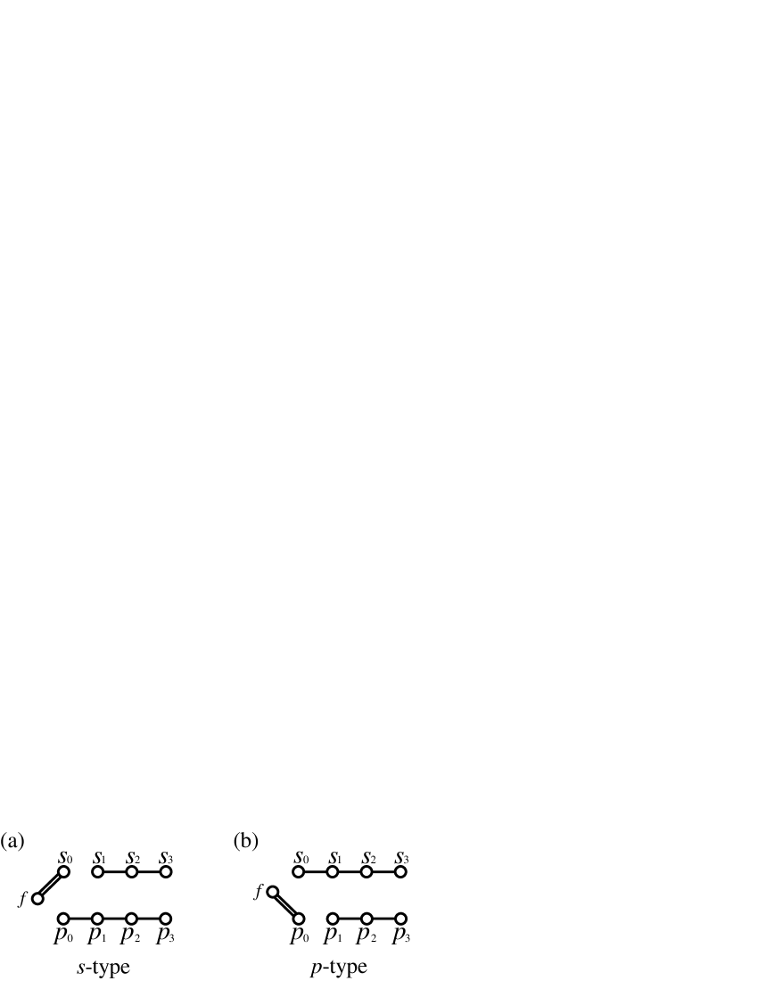
Figure 3: (Color online) Graphical representations of the two types of the energy spectra.

Now let us discuss the fixed points for the present model. After $n$ steps in the NRG, the system consists of $2n+3$ sites, the localized $f$ orbital and the two Wilson chains, $s_{0}$, $s_{1}$, $\cdots$, $s_{n}$ and $p_{0}$, $p_{1}$, $\cdots$, $p_{n}$. Our numerical results by the NRG method show that there are only two stable fixed points: $s$- and $p$-type. The $s$-type fixed point schematically shown in Fig. 3(a) is characterized by the energy spectrum which is isomorphic to that of the system composed of tightly bound $f-s_{0}$ singlet and two independent Wilson chains whose length is different, $n$ sites for the $s$-chain and $n+1$ sites for the $p$-chain. It is important to include the parity as a quantum number, $[N^{\text{tot}}$, $S^{\text{tot}}_{z}$, $P]$. Concerning the $s$-type fixed point the phonon part does not play any important role and the total parity $P$ is simply determined by the number of electrons in the $p$-channel. From Fig. 3(a) it is straightforward to see that the quantum numbers of the degenerate ground states are those given in Table 1 depending on even or odd $n$. As an example, we show in Table 2 a part of the low energy spectra of the $s$-type fixed point which correspond to the one particle excited states. The other fixed point defined as $p$-type is depicted in Fig. 3(b). The energy spectrum at low energies is isomorphic to that for the system with isolated $f-p_{0}$ singlet bond and two independent Wilson chains, $n+1$ sites for the $s$-chain and $n$ sites for the $p$-chain. One important non-trivial fact obtained by the present NRG calculations is that the quantum number for the part of $f-p_{0}$ singlet is always given by $[2$, $0$, $1]$, odd parity in the same way as the two-site problem discussed in §3.2. Therefore the quantum numbers of the ground states for the entire system are given by those shown in Table 1.

		NRG step $n$
		even	odd
fixed point	$s$-type	$[2n+2$, $0$, $0]$	$[2n+2$, $0$, $0]$
		$[2n+3$, $\pm\frac{1}{2}$, $1]$	$[2n+3$, $\pm\frac{1}{2}$, $0]$
		$[2n+4$, $0$, $0]$	$[2n+4$, $0$, $0]$
	$p$-type	$[2n+2$, $0$, $1]$	$[2n+2$, $0$, $1]$
		$[2n+3$, $\pm\frac{1}{2}$, $1]$	$[2n+3$, $\pm\frac{1}{2}$, $0]$
		$[2n+4$, $0$, $1]$	$[2n+4$, $0$, $1]$

Table 1: Sets of $[N^{\text{tot}},$ $S^{\text{tot}}_{z},$ $P]$ of the ground states at the $n$-th NRG step depending on the types of the fixed points.

$s$-type fixed point
	$[1,$ $0,$ $0]$		$[1,$ $0,$ $1]$
0th	$0$	$1$	$0.800048$	2
1st	$1.600095$	$3$	$2.400143$	2
2nd	$1.695754$	$2$	$2.495802$	6
3rd	$3.200191$	$1$	$2.997488$	2

Table 2: The low energy spectra of the $s$-type fixed point at an even number of the NRG steps for the sets of the quantum numbers, $[1,$ $0,$ $0]$ and $[1,$ $0,$ $1]$. In this table, $N^{\text{tot}}$ is counted from the total number of sites. The energy eigenvalues and their degeneracy factors are tabulated up to the third excited states. The low energy spectra of the $p$-type fixed point can be obtained by the inversion of the total parity $P$.

Lastly, we discuss the unstable fixed points which separate the regions of the $s$- and $p$-type fixed points. Here, we briefly review the $2$-channel Kondo model. The model consists of a local moment coupled antiferromagnetically with two types of conduction electrons[32, 33, 34]. The NRG calculations show that 2-channel Kondo effect is realized when the two antiferromagnetic coupling constants, $J_{a}$ and $J_{b}$, are perfectly equal[33]. The energy spectra obtained from the NRG calculations are summarized in Refs. References and References. The low-energy spectrum of the $2$-channel Kondo model with $J_{a}=J_{b}$ shows $SO(5)$ rotational symmetry, in the sense that the degeneracy factors of the eigenstates are subject to dimensions of its irreducible representations.

Returning back to the present Hamiltonian, it is confirmed that the spectra of low-energy eigenvalues on the unstable fixed points are identical to those obtained for the $2$-channel Kondo model with $J_{a}=J_{b}$, see Table 3. Therefore, we describe these unstable fixed points as the $2$-channel Kondo ($2$-chK) ones.

Present model	$2$-channel Kondo model
$[Q,$ $S^{\text{tot}}_{z},$ $P]$	$(Q,$ $S,$ $S_{\text{ch}})$	$SO(5)$	$E_{\text{NRG}}$
$[0,$ $\frac{1}{2},$ $1]$	$(0,$ $\frac{1}{2},$ $0)$	1	$0$
$[\pm 1,$ $0,$ $0]$	$(\pm 1,$ $0,$ $\frac{1}{2})$	4	$0.125$
$[\pm 1,$ $0,$ $1]$
$[\pm 2,$ $\frac{1}{2},$ $0]$	$(\pm 2,$ $\frac{1}{2},$ $0)$	5	0.505
$[0,$ $\frac{1}{2},$ $0]^{*}$	$(0,$ $\frac{1}{2},$ $1)$
$[0,$ $\frac{1}{2},$ $1]$
$[\pm 1,$ $0,$ $0]$	$(\pm 1,$ $1,$ $\frac{1}{2})$	$4$	$0.637$
$[\pm 1,$ $0,$ $1]$
$[0,$ $\frac{1}{2},$ $1]$	$(0,$ $\frac{3}{2},$ $0)$	$1$	$1.013$

Table 3: Correspondence relation of the low energy eigenstates of the $2$-chK fixed point between the present model and the $2$-channel Kondo model at an even number of the NRG steps. In this table, $Q$ is defined by the difference between $N^{\text{tot}}$ and the total number of sites. Spin degeneracy is not counted in this table. The right part of the table is from Table 12 in Ref. References with spin $S$ and channel spin $S_{\text{ch}}$ for the 2-channel Kondo model. *There are doubly degenerate states.

4.2 Phase diagram of the generalized Anderson model for a vibrating magnetic ion

From the energy spectra obtained by the NRG calculations, we determine the ground-state phase diagram which is shown in Fig. 4. The parameter space is divided into two distinct areas. The left part is characterized by the $s$-type energy spectrum and the right part by the $p$-type one. On the boundary, the energy spectrum is of the $2$-chK type. On the line of $U=0$, the $s$-type energy spectrum always appears. Therefore the line of $2$-chK fixed points does not merge together to the $U=0$ line but approaches it asymptotically.

The NRG calculations reveal that physical properties of the system at finite temperatures are sometimes quite different even if two different sets of parameters belong to the region of the same fixed point at zero temperature. Therefore, in addition to the analysis of the low temperature energy spectra, we have to investigate finite temperature behaviors of physical quantities at each point of the parameter space.

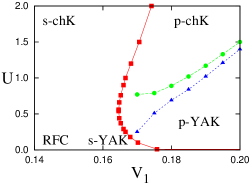
Figure 4: (Color online) The phase diagram in the parameter space of $V_{1}$ and $U$ for $V_{0}=\omega=0.2$. On the boundary, the energy spectrum is of the $2$-chK type. The left region is characterized by the $s$-type energy spectra and the right one by the $p$-type one. In the region between the green and blue dashed lines, the plateau of $S_{\text{imp}}$ at $k_{\text{B}}\log 2$ disappears.

First, we focus on the left side of the $2$-chK line. On the line of $U=0$ this model is equivalent to the spinful YA model. In the weak electron-phonon coupling regime main source of kinetic energy comes from the hybridization with the $s$-wave conduction electrons and the phonon-assisted hybridization with the $p$-wave channel is a weak perturbation. In this paper we characterize this regime by the renormalized Fermi chain (RFC). When $V_{1}$ increases, the PD is formed and the degeneracy is lifted at low temperatures by the Yu and Anderson type Kondo effect, expressed as $s$-YAK in Fig. 4. Now, we gradually increase Coulomb interaction $U$, starting from the parameter region where temperature dependence of physical quantities is of the RFC type. The impurity begins to behave as a localized spin and then the spin is screened mainly by the $s$-wave conduction electrons. This regime is called $s$-channel Kondo ($s$-chK) in Fig. 4. In the parameter region between RFC and $s$-chK, the essence of the physics can be understood based on the local Fermi liquid theory[36, 37].

Next, we discuss the right part of the phase diagram. Concerning the strong $U$ regime, it is easy to understand that the local moment is screened mainly by the $p$-wave conduction electrons, which is called $p$-channel Kondo ($p$-chK). When $U$ is not important compared with $V_{1}$, the picture of the PD is valid, while the temperature dependence of physical quantities is different from that in the $s$-YAK parameter region in addition to the difference in the energy spectra. We denote this region as $p$-YAK in Fig. 4. In the following subsections, we will discuss details of physical properties for various parameters, including the difference between the $s$-YAK and $p$-YAK.

4.3 Three-site problem

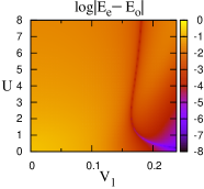
Figure 5: (Color online) The line of level crossing in the parameter space of $V_{1}$ and $U$ obtained from the three-site two-electron problem for $V_{0}=\omega=0.2$. The color grade corresponds to the magnitude of $\log|E_{\text{e}}-E_{\text{o}}|$, where $E_{\text{e}}$ and $E_{\text{o}}$ are the ground state energies with even and odd parity, respectively. In the left part of the deep blue line, $E_{\text{e}}$ is lower than $E_{\text{o}}$.

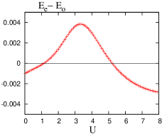
Figure 6: (Color online) $U$ dependence of the difference between $E_{\text{e}}$ and $E_{\text{o}}$ for the three-site problem with two electrons: $V_{0}=\omega=0.2$ and $V_{1}=0.174$.

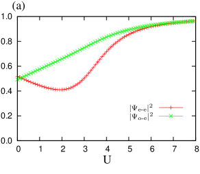
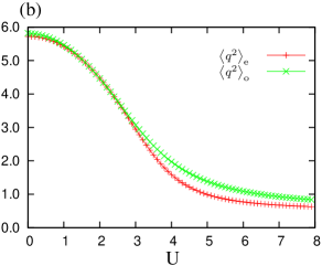
Figure 7: (Color online) (a) $U$ dependence of $|\Psi_{\text{e-e}}|^{2}$ and $|\Psi_{\text{o-e}}|^{2}$ obtained for the three-site two-electron problem with $V_{0}=\omega=0.2$ and $V_{1}=0.174$. (b) $U$ dependence of $\bigl{<}q^{2}\bigr{>}_{\text{e}}$ and $\bigl{<}q^{2}\bigr{>}_{\text{o}}$, which are the expectation values of the square of the ion displacement calculated from $\Psi_{\text{even}}$ and $\Psi_{\text{odd}}$.

At this point, it is instructive to consider the three-site problem, which consists of $f$, $s_{0}$ and $p_{0}$ sites. The Hamiltonian is given by

$$\mathit{H}_{\text{3-site}}= \ \ \ \ V_{0}\sum_{\sigma}\bigl{\{}s^{\dagger}_{\sigma}f_{\sigma}+\text{h.c.}\bigr{\}}$$

$$+V_{1}\sum_{\sigma}\bigl{\{}p^{\dagger}_{\sigma}f_{\sigma}+\text{h.c.}\bigr{\}}(a+a^{\dagger})+\hbar\omega a^{\dagger}a$$

$$+\frac{U}{2}\biggl{(}\sum_{\sigma}f^{\dagger}_{\sigma}f_{\sigma}-1\biggr{)}^{2},$$ (4.1)

where the site suffix $"0"$ is suppressed. It is easy to obtain the exact eigenvalues and eigenstates by using the exact diagonalization method. In the following examples the number of phonon excitations is kept up to $50$ and $V_{0}$ and $\omega$ are fixed to $0.2$.

Figure 5 shows the magnitude of $\log|E_{\text{e}}-E_{\text{o}}|$ in the two-dimensional parameter space of $V_{1}$ and $U$, where $E_{\text{e}}$ $(E_{\text{o}})$ is the ground state energies with even and odd parity. In the figure there is a line of level crossing between $E_{\text{e}}$ and $E_{\text{o}}$. In the left (right) part of the line, $E_{\text{e}}$ $(E_{\text{o}})$ is lower than $E_{\text{o}}$ $(E_{\text{e}})$. Figure 6 shows $U$ dependence of the difference between $E_{\text{e}}$ and $E_{\text{o}}$ with $V_{1}$ fixed to $0.174$. Clearly there is similarity between Fig. 4 and Fig. 5.

From the view point of parity, every component of wave functions is classified into four groups, $\Psi_{\text{e-e}}$, $\Psi_{\text{e-o}}$, $\Psi_{\text{o-e}}$ and $\Psi_{\text{o-o}}$. $\Psi_{\text{e-o}}$, for example, means a linear combination of the components whose electron parts have even parity and phonon parts odd parity. Clearly an eigenstate with even total parity is written as

$$\Psi_{\text{even}} =\Psi_{\text{e-e}}+\Psi_{\text{o-o}},$$ (4.2)

while one with odd total parity as

$$\Psi_{\text{odd}} =\Psi_{\text{o-e}}+\Psi_{\text{e-o}}.$$ (4.3)

Concerning the three-site two-electron problem, the bases for a given parity are listed in Table 4.

Figure 7(a) shows $U$ dependence of the amplitudes, $|\Psi_{\text{e-e}}|^{2}$ and $|\Psi_{\text{o-e}}|^{2}$, for $V_{1}=0.174$. Because the total wave functions are normalized, $|\Psi_{\text{o-o}}|^{2}=1-|\Psi_{\text{e-e}}|^{2}$ and $|\Psi_{\text{e-o}}|^{2}=1-|\Psi_{\text{o-e}}|^{2}$. In Fig. 7(b) we show the expectation values of the square of the ion displacement, $\bigl{<}q^{2}\bigr{>}_{\text{e}}$ and $\bigl{<}q^{2}\bigr{>}_{\text{o}}$, which are calculated from $\Psi_{\text{even}}$ and $\Psi_{\text{odd}}$, respectively.

We start from the two-site problem for the non-interacting case, namely $V_{0}=U=0$, where the ground states $|+\bigl{>}$ and $|-\bigl{>}$ or $|\text{L}\bigl{>}$ and $|\text{R}\bigl{>}$ are doubly degenerate. When $V_{0}$ is introduced, we expect that the kinetic energy favors the configurations which belong to $\Psi_{\text{e-e}}$. Actually, the amplitude $|\Psi_{\text{e-e}}|^{2}$ shown in Fig. 7(a) is larger than $0.5$ at $U=0$. As we have discussed in §3.2 the Coulomb interaction $U$ favors the state with odd total parity. The competition leads to the level crossing at small $U$.

	Parity $P$
	0	1
electron	$s^{\dagger}_{\uparrow}s^{\dagger}_{\downarrow}|\text{vac}\bigr{>}_{\text{el}}$
	$f^{\dagger}_{\uparrow}s^{\dagger}_{\downarrow}|\text{vac}\bigr{>}_{\text{el}}$, $s^{\dagger}_{\uparrow}f^{\dagger}_{\downarrow}|\text{vac}\bigr{>}_{\text{el}}$	$s^{\dagger}_{\uparrow}p^{\dagger}_{\downarrow}|\text{vac}\bigr{>}_{\text{el}}$, $p^{\dagger}_{\uparrow}s^{\dagger}_{\downarrow}|\text{vac}\bigr{>}_{\text{el}}$
	$f^{\dagger}_{\uparrow}f^{\dagger}_{\downarrow}|\text{vac}\bigr{>}_{\text{el}}$, $p^{\dagger}_{\uparrow}p^{\dagger}_{\downarrow}|\text{vac}\bigr{>}_{\text{el}}$	$f^{\dagger}_{\uparrow}p^{\dagger}_{\downarrow}|\text{vac}\bigr{>}_{\text{el}}$, $p^{\dagger}_{\uparrow}f^{\dagger}_{\downarrow}|\text{vac}\bigr{>}_{\text{el}}$
phonon	$|n\bigr{>}_{\text{ph}}$ $(n=$ even$)$	$|n\bigr{>}_{\text{ph}}$ $(n=$ odd$)$

Table 4: Bases for electron and phonon parts of the three-site two-electron problem classified by the parity $P$.

In the narrow region of $V_{1}$, the ground state makes the second level crossing at larger $U$. In the strongly correlated regime, a local moment is formed in the $f$-orbital, which should be eventually screened by the conduction electrons. The expectation values of square of the ion displacement are suppressed and become close to the amplitude of zero point fluctuations for both $\Psi_{\text{even}}$ and $\Psi_{\text{odd}}$ as shown in Fig. 7(b). In this situation, the phonon parts of the wave functions are dominated by components with even phonon numbers. This fact is clearly seen in Fig. 7(a). Therefore the total parity is predominantly determined by the nature of singlet formation, even parity for the $f-s$ singlet while odd parity for the $f-p$ singlet. The upper critical $U$ shown in Fig. 6 corresponds to the point where the two screening mechanisms compete in the same way as the $2$-chK fixed point shown in the phase diagram for the bulk system, Fig. 4.

The line of level crossing shown in Fig. 5 is qualitatively very similar to the phase boundary obtained by the NRG calculations, Fig. 4. We would like to point out that the three-site Hamiltonian corresponds to the initial step of the NRG procedure and the ground state of the two-electron problem has the different parity depending on the nature of the singlet bond as discussed in §4.1, see also Table 1.

4.4 Strong correlation regime $(U\gg\omega\gg T)$

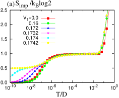
Figure 8: (Color online) Temperature dependence of entropy in the strong correlation regime. The used parameters are $V_{0}=\omega=0.2$ with the symmetric condition $U=-2\varepsilon_{f}=2.0$. (a) For $V_{1}<0.1742$, the $s$-chK effect is observed. (b) When $V_{1}$ is larger than the critical value the local moment is mainly screened by the $p$-wave conduction electrons, corresponding to the $p$-chK effect. At $V_{1}=0.1742$, we observe signature of the $2$-channel Kondo effect.

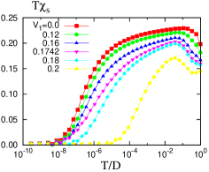
Figure 9: (Color online) Temperature dependence of spin susceptibility $T\chi_{s}$ in the strong correlation regime, $V_{0}=\omega=0.2$ with the symmetric condition $U=-2\varepsilon_{f}=2.0$. When $V_{1}$ is relatively small, $T\chi_{s}$ increases close to 0.25 which corresponds to the local moment limit. With increasing $V_{1}$, phonon-assisted hybridization suppresses the enhancement of $T\chi_{s}$.

Firstly, we discuss physical properties in the strong $U$ regime where the relation, $U\gg\omega\gg T$, holds. In this regime multi phonon excitation processes are not important. Because of the strong $U$, the localized orbital behaves as a local moment which is coupled with the $s$-wave and $p$-wave conduction electrons. With lowering temperature, the local moment is screened by the conduction electrons and the main screening channel changes depending on relative strength between $V_{0}$ and $V_{1}$. In the same way as the conventional impurity Anderson model is mapped to the spin $1/2$ Kondo model[38], we consider the projected Hilbert space where the vacuum and doubly occupied states of the impurity orbital are prohibited. We treat both of the conventional hybridization term $V_{0}$ and the phonon-assisted one $V_{1}$ in the Hamiltonian (2.9) as perturbation terms. After some calculations, a generalized Kondo model is obtained as

$$\mathit{H}_{\text{Kondo}}= \sum_{k\sigma}\sum_{\ell=0,1}\varepsilon(k)c^{\dagger}_{\ell\sigma}(k)c_{\ell\sigma}(k)+\hbar\omega a^{\dagger}a+\mathit{H}_{\text{s-d}},$$

$$\mathit{H}_{\text{s-d}}= -{\sum_{kk^{\prime}}}\sum_{\alpha\beta}\biggl{\{}J_{0,0}c^{\dagger}_{0\alpha}(k)\bigl{[}\bm{\sigma}\bigr{]}_{\alpha\beta}c_{0\beta}(k^{\prime})\cdot\mathbf{S}$$

$$+J_{1,0}~{}q\bigl{[}c^{\dagger}_{1\alpha}(k)\bigl{[}\bm{\sigma}\bigr{]}_{\alpha\beta}c_{0\beta}(k^{\prime})\cdot\mathbf{S}+\text{h.c.}\bigr{]}$$

$$+J_{1,1}~{}q^{2}c^{\dagger}_{1\alpha}(k)\bigl{[}\bm{\sigma}\bigr{]}_{\alpha\beta}c_{1\beta}(k^{\prime})\cdot\mathbf{S}\biggr{\}},$$ (4.4)

where $\mathbf{S}=f^{\dagger}_{\alpha}[\bm{\sigma}]_{\alpha\beta}f_{\beta}$ with $\bm{\sigma}$ being the vector of Pauli matrices and $q=(a+a^{\dagger})/\sqrt{2}$. The coupling constants $J_{0,0}$, $J_{1,0}$ and $J_{1,1}$ are written as

$$J_{0,0}\equiv V^{2}_{0}\biggl{\{}\frac{1}{\varepsilon_{f}}-\frac{1}{\varepsilon_{f}+U}\biggr{\}},$$

$$J_{1,0}\equiv V_{0}\bigl{(}\sqrt{2}V_{1}\bigr{)}\biggl{\{}\frac{1}{\varepsilon_{f}}-\frac{1}{\varepsilon_{f}+U}\biggr{\}},$$

$$J_{1,1}\equiv 2V^{2}_{1}\biggl{\{}\frac{1}{\varepsilon_{f}}-\frac{1}{\varepsilon_{f}+U}\biggr{\}}.$$

The term proportional to $J_{1,0}$ corresponds to scattering processes from the $s$-wave conduction electrons to the $p$-wave ones and vice versa. Similarly, the term proportional to $J_{1,1}$ describes scattering processes within the $p$-wave conduction electrons. In the strong correlation regime, effects of electron-phonon coupling are suppressed by Coulomb interaction. Therefore we may regard the effects of phonon emission or absorption processes as a renormalization of the coupling constant by taking average over the phonon degree of freedom,

$$\mathit{H}_{\text{s-d}}\simeq -{\sum_{kk^{\prime}}}\sum_{\alpha\beta}\bigl{\{}J_{0,0}c^{\dagger}_{0\alpha}(k)\bigl{[}\bm{\sigma}\bigr{]}_{\alpha\beta}c_{0\beta}(k^{\prime})\cdot\mathbf{S}$$

$$+J_{1,1}\bigl{<}q^{2}\bigr{>}c^{\dagger}_{1\alpha}(k)\bigl{[}\bm{\sigma}\bigr{]}_{\alpha\beta}c_{1\beta}(k^{\prime})\cdot\mathbf{S}\bigr{\}},$$ (4.5)

where used is the fact that $\bigl{<}q\bigr{>}$, the thermal averages of $q$, vanishes. Even if the electron-phonon coupling is weak, $\bigl{<}q^{2}\bigr{>}$ is not zero due to the zero point fluctuations.

In Figs. 8 and 9 we use a set of parameters, $V_{0}=\omega=0.2$ with the symmetric condition $U=-2\varepsilon_{f}=2.0$. When $V_{1}$ is relatively small, the local moment is mainly screened by the $s$-channel conduction electrons, corresponding to the $s$-channel Kondo effect. Figure 8(a) shows that entropy of the impurity site $S_{\text{imp}}$ is not affected so much by the $p$-wave conduction electrons for $V_{1}\leq 0.16$. Spin susceptibility $T\chi_{s}$ shown in Fig. 9 reaches close to $0.25$ of the local moment limit because of strong $U$. At the critical $V_{1}(=0.1742)$, the energy spectra are characterized by the $2$-channel Kondo fixed point and accordingly the plateau of entropy at $(1/2)k_{\text{B}}\log 2$ appears at low temperatures. When $V_{1}$ is larger than the critical value, a different type of Kondo effect takes place through screening by the $p$-wave conduction electrons as shown in Fig. 8(b). With further increase of $V_{1}$, effective Coulomb interaction at the impurity site is suppressed by the electron-phonon coupling. This effect of renormalization of effective Coulomb interaction appears as the higher Kondo temperatures in Fig. 8(b) and also as the suppression of $T\chi_{s}$ in Fig. 9.

At the $2$-channel Kondo fixed point, the thermal average of square of ion displacement $\bigl{<}q^{2}\bigr{>}$ converges to $0.739$ at low temperatures. When we substitute the number into $\bigl{<}q^{2}\bigr{>}$, the ratio of $J_{1,1}\bigl{<}q^{2}\bigr{>}$ to $J_{0,0}$ is estimated to be

$$\frac{J_{1,1}\bigl{<}q^{2}\bigr{>}}{J_{0,0}}\simeq 1.12.$$ (4.6)

The estimated value close to $1$ seems to be reasonable.

4.5 Non-interacting case $(U=0)$

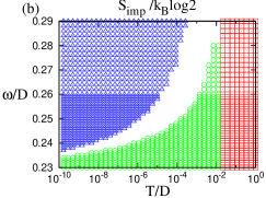
Figure 10: (Color online) Temperature dependence of entropy for various phonon frequency $\omega$ with $V_{0}=V_{1}=0.2$ and $U=0$. When $\omega$ is small, $S_{\text{imp}}$ shows a plateau at $k_{\text{B}}\log 2$. For $\omega<0.28$, the plateau due to the PD is suppressed in the same temperature dependence as the usual Kondo effect. Results on the entropy for various $\omega$ are assembled in the parameter plane of $\omega$ and $T$ in the lower panel. The red squares are the points where the entropy is larger than $1.1k_{\text{B}}\log 2$ and the green circles are for $0.9k_{\text{B}}\log 2<S_{\text{imp}}<1.1k_{\text{B}}\log 2$ and the blue triangles for $S_{\text{imp}}<0.1k_{\text{B}}\log 2$.

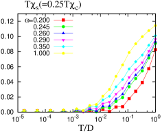
Figure 11: (Color online) Temperature dependence of spin susceptibility $T\chi_{s}(=0.25T\chi_{c})$ for $V_{0}=V_{1}=0.2$ and $U=0$. When $\omega$ is lowered, $T\chi_{s}(=0.25T\chi_{c})$ is suppressed since strong electron-phonon coupling increases the binding energy of the PD.

Figure 12: (Color online) Thermal average of square of ion displacement, $\bigl{<}q^{2}\bigr{>}$, for $V_{0}=V_{1}=0.2$ and $U=0$. When $\omega$ becomes larger, $\bigl{<}q^{2}\bigr{>}$ asymptotically comes close to $0.5$ which corresponds to the zero point fluctuation.

For discussions on the non-interacting case we fix the set of parameters $V_{0}=V_{1}=0.2$ and $U=0.0$. In this subsection we use frequency of phonon $\omega$ as a parameter to change the strength of electron-phonon coupling, which is an alternative to control $V_{1}$ with a fixed $\omega$.

Entropy of the impurity site $S_{\text{imp}}$ is shown in Fig. 10(a) for various $\omega$. As $\omega$ decreases, the plateau of entropy at $k_{\text{B}}\log 2$ develops owing to the formation of the PD. Figure 10(b) summarizes results on the entropy in $\omega-T$ plane. Typical YAK behaviors are observed in the parameter range from $\omega=0.238$ to $0.280$. The middle of the blank area between the blue triangle and green circle regions corresponds to the Kondo temperature for the YAK effect.

In Fig. 11 the spin (charge) susceptibility of the impurity, $T\chi_{s}$ $(T\chi_{c})$, is shown for various $\omega$. In general the relation $T\chi_{s}=0.25T\chi_{c}$ holds in the non-interacting cases. When temperature is lower than the binding energy of the PD, $E_{\text{PD}}$, spin and charge fluctuations at the impurity site are suppressed due to the formation of the PD which consists of the spin singlets of doubly occupied bonding or anti-bonding states. Therefore, unlike the usual spin Kondo effect temperature dependence of $T\chi_{s}$ ($T\chi_{c}$) is governed by $E_{\text{PD}}$ rather than the Kondo temperature of the YAK effect.

Figure 12 shows temperature dependence of the thermal average of square of ion displacement, $\bigl{<}q^{2}\bigr{>}$. For all $\omega$, $\bigl{<}q^{2}\bigr{>}$ converges to a constant at low temperatures and does not show any changes in the vicinity of the YAK temperature. Once the PD is formed the phonon states are almost frozen and given by the two distinct coherent states which are symmetrically shifted right and left from the center. It is interesting to note that $\bigl{<}q^{2}\bigr{>}$ for $\omega$=$0.230$, $0.245$ and $0.260$ show minima in the temperature range from $10^{0}$ to $10^{-2}$ which may correspond to $E_{\text{PD}}$. These behaviors may be interpreted as formation of the effective double-well potential for the ion displacement. When temperature is higher than $E_{\text{PD}}$, the dynamics of the ion is governed by the original harmonic cage potential. On the other hand, below the energy scale of $E_{\text{PD}}$, the ion tunnels between the left and right minima corresponding to $|\text{L}\bigl{>}$ and $|\text{R}\bigl{>}$.

4.6 Effect of finite $U$ in the weak electron-phonon coupling regime

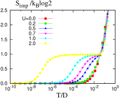
Figure 13: (Color online) Temperature dependence of entropy in the weak electron-phonon coupling regime, $V_{0}=2V_{1}=\omega=0.2$. When $U$ is increased, a plateau of entropy at $k_{\text{B}}\log 2$ appears because of formation of the local moment. At low temperatures the local moment is screened mainly by the $s$-wave conduction electrons.

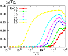
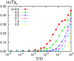
Figure 14: (Color online) Temperature dependence of $T\chi_{s}$ shown in the upper panel and $T\chi_{c}$ in the lower one in the weak electron-phonon coupling regime, $V_{0}=2V_{1}=\omega=0.2$. The relation, $T\chi_{s}=0.25T\chi_{c}$, is valid for $U=0$. When $U$ is increased, $T\chi_{s}$ is enhanced while $T\chi_{c}$ is suppressed.

Next we choose the set of parameters $V_{0}=2V_{1}=\omega=0.2$, where screening by the $s$-wave conduction electrons dominates over the $p$-wave ones. To investigate the effects of Coulomb interaction, we show temperature dependence of the physical quantities, the entropy of the impurity ion $S_{\text{imp}}$ in Fig. 13, the spin susceptibility $T\chi_{\text{s}}$ in Fig. 14(a) and the charge susceptibility $T\chi_{\text{c}}$ in Fig. 14(b). When $U$ is small, $S_{\text{imp}}$ monotonically decays to zero. $T\chi_{s}$ and $T\chi_{c}$ also go to zero without any plateau. Therefore, we conclude that the physical properties correspond to the RFC regime in Fig. 4. When $U$ increases, the impurity orbital begins to behave as a local moment. Actually, the plateau region in Fig. 13 is broadened with increasing $U$. Correspondingly, $T\chi_{s}$ is enhanced and shows a maximum close to $0.25$ while $T\chi_{c}$ is suppressed, which are signatures of a local moment. As already mentioned, the energy spectra are characterized by the $s$-type fixed point for any $U$. However the physical properties cross over from the RFC behaviors to the $s$-chK ones with increasing $U$.

4.7 Effect of finite $U$ in the strong electron-phonon coupling regime

Figure 15: (Color online) (a)Temperature dependence of entropy $S_{\text{imp}}$ for $U\leq 1.2$ in the strong electron-phonon coupling regime, $V_{0}=V_{1}=\omega=0.2$. Plateaus at $k_{\text{B}}\log 2$ originate from the degeneracy of the PD. At $U=0$ the binding energy of the PD is so large that Yu and Anderson type Kondo temperature is lower than $10^{-10}$. For finite $U$, the degeneracy of the PD is lifted by the Coulomb interaction. (b)Temperature dependence of $S_{\text{imp}}$ for $U=0.01$ and its fit by a Shottoky type entropy with the excitation gap $\Delta=3.9\times 10^{-5}$.

Figure 16: (Color online) Temperature dependence of entropy $S_{\text{imp}}$ for $U\geq 1.4$ in the strong electron-phonon coupling regime, $V_{0}=V_{1}=\omega=0.2$. Plateaus at $k_{\text{B}}\log 2$ come from the degeneracy of the local moment for the relatively strong $U$. The low temperature energy spectra are characterized by the $p$-type.

In this subsection we show results of NRG calculations for a strong electron-phonon coupling case, $V_{0}=V_{1}=\omega=0.2$. In Figs. 15(a) and 16 we see two distinct temperature dependence of $S_{\text{imp}}$ in the course of release of entropy from the plateau at $k_{\text{B}}\log 2$.

For $U<1.4$ shown in Fig. 15(a), the electron-phonon coupling is relatively more important than the Coulomb interaction. In this region, the Coulomb interaction can be treated as a perturbation to the PD.

For the non-interacting case the plateau of entropy at $k_{\text{B}}\log 2$ is not suppressed even at low temperatures. Because of the strong electron-phonon coupling we expect that the YAK temperature is much lower than $10^{-10}$.

For $U>0$, the low temperature energy spectrum is of the $p$-type. In §3.2, we showed that the Coulomb interaction lifts the degeneracy of the PD in a similar way as a transversal magnetic field lifts degeneracy of a free spin. When $U$ is smaller than $1.4$, it is expected that low-energy physics of the impurity is identified as Yu and Anderson type Kondo effect under the ”transverse field”, which is characterized by $p$-YAK in the phase diagram, Fig. 4. Therefore, it is useful for us to compare the present results with those of conventional spin $1/2$ Kondo model under magnetic field. It is shown for the latter model that when the magnetic field is larger than Kondo temperature behavior of heat capacity approaches to a Schottky form (see Fig. 15 in Ref. References). The lower panel of Fig. 15 shows $S_{\text{imp}}$ at $U=0.01$ fitted by the Schottky form with $\Delta=3.9\times 10^{-5}$. Let us compare this $\Delta$ with the energy gap between the PD, namely $\Delta_{\text{PD}}$. To estimate $\Delta_{\text{PD}}$ it is appropriate to use a renormalized coupling constant $\lambda^{{}^{\prime}}$ instead of the bare $\lambda(\equiv-V_{1}/\omega)$. We can estimate $\lambda^{{}^{\prime}}$ from the NRG calculations by using the relation $\bigl{<}q^{2}\bigr{>}\equiv(16{\lambda^{{}^{\prime}}}^{2}+1)/2$. In this way $\Delta_{\text{PD}}$ is estimated to be $2.62\times 10^{-5}$ for $U=0.01$ by using $\bigl{<}q^{2}\bigr{>}=5.75$. It is important to note that there is a notable deviation at low temperatures from the Schottky form. It indicates that energy spectrum at low temperatures is not gapped but continuous, which is consistent with the fact that even with a finite $U(\neq 0)$ the low temperature properties are described by a local Fermi liquid coupled with the $p$-wave conduction electrons.

We comment on the transition from the $s$-YAK regime to the $p$-YAK regime in the case of strong electron-phonon coupling. Let us start from the noninteracting case, $U=0$. As we have discussed in §4.5 Kondo temperature of the YAK effect $T_{\text{YAK}}$ is generally small and becomes extremely small as the binding energy $|E_{\text{PD}}|$ gets larger, see Fig. 10(b). The Kondo energy, $k_{\text{B}}T_{\text{YAK}}$, is nothing but the energy gain at the $s$-type fixed points. On the other hand, the Coulomb interaction is favorable to the $p$-type fixed points and $\Delta_{\text{PD}}$ is its energy gain. Therefore, the transition takes place when $k_{\text{B}}T_{\text{YAK}}\sim\Delta_{\text{PD}}$. Since $k_{\text{B}}T_{\text{YAK}}$ is extremely small for strong electron-phonon coupling, the transition takes place close vicinity of the $U=0$ line.

For $U\geq 1.5$ electrons in the impurity orbital behave as a local moment and it is quenched dominantly by the $p$-wave conduction electrons. Actually, in Fig. 16 there are plateaus of entropy at $k_{\text{B}}\log 2$ and the entropy is released in the same temperature dependence as the usual Kondo effect.

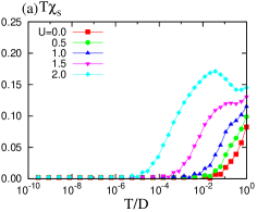
Figure 17: (Color online) Temperature dependence of $T\chi_{s}$ (a) and $T\chi_{c}$ (b) in the strong electron-phonon coupling regime, $V_{0}=V_{1}=\omega=0.2$. For the $U=0$, the relation $T\chi_{s}=0.25T\chi_{c}$ is valid. Unlike the weak electron-phonon coupling case, the enhancement of $T\chi_{s}$ by Coulomb interaction is weak for $U<2.0$. $T\chi_{s}$ starts to show a maximum for $U>2.0$ and becomes close to 0.25 as $U$ is increased.

Lastly, let us discuss the intermediate parameter region, see Fig. 4. In the region between green and blue dashed lines, the entropy decays to zero without any plateau. It seems that the Coulomb interaction and the electron-phonon coupling are competing and almost balanced each other, leading to almost monotonic temperature dependence of $T\chi_{s}$ as shown in Fig. 17(a) and $T\chi_{c}$ in (b). Of course the energy spectra at low temperatures are always characterized by the $p$-type except for $U=0.0$. However the nature of the physical properties changes from the PD with a small energy splitting due to the Coulomb interaction for $U\leq 1.4$ to the local moment regime for $U\geq 1.5$. The crossover between the two regimes is rapid but continuous.

4.8 The line of 2-channel Kondo fixed points

Figure 18: (Color online) $U$ versus $\bigl{<}q^{2}\bigr{>}$ and $\bigl{<}\bm{S}^{2}_{f}\bigr{>}$ with $V_{0}=\omega=0.2$. The sets of the parameters, $V_{1}$ and $U$, are chosen to correspond to each points on the red line with squares in Fig.4.

Finally we discuss physical properties on the line of $2$-channel Kondo fixed points shown in Fig. 4. On the line, energy spectra are always characterized by the $2$-chK type. For the strong Coulomb interaction regime, the effective Hamiltonian is given by eq. (4.4), which is equivalent to the conventional $2$-chK model. It is well known that the $2$-chK effect is realized when the two types of screening channels are fully balanced. In the weak correlation regime, however, the degrees of freedom screened by the conduction electrons are not the spin degrees of freedom of the impurity orbital but the ion displacements of the PD.

To observe the crossover behavior, we show thermal average of square of the ion displacement $\bigl{<}q^{2}\bigr{>}$ and magnitude of the local moment $\bigl{<}\bm{S}^{2}_{f}\bigr{>}$ calculated at low temperatures. Figure 18 shows $\bigl{<}q^{2}\bigr{>}$ and $\bigl{<}\bm{S}^{2}_{f}\bigr{>}$ calculated for the sets of parameters on the line of $2$-chK fixed points in Fig. 4. When $U$ increases along the line, $\bigl{<}q^{2}\bigr{>}$ is suppressed by Coulomb interaction and approaches to $0.5$ which corresponds to the zero point fluctuations. $\bigl{<}q^{2}\bigr{>}$ decreases monotonically, showing a concave curve as a function of $U$. On the other hand, the magnitude of the local moment $\bigl{<}\bm{S}^{2}_{f}\bigr{>}$ increases from 0.375 to $0.75$. The former number corresponds to the free orbital limit, while the latter to the local moment limit. The curve of $\bigl{<}\bm{S}^{2}_{f}\bigr{>}$ is concave-downward. These results support the view that the degree of freedom to be screened by conduction electrons smoothly transfers from the ion displacement to the spin degrees of freedom of local moment with increasing $U$.

5 Conclusion and future problems

In this paper we have discussed Kondo effects when a magnetic ion is vibrating in a harmonic potential. The central issue is the competition between the Coulomb and electron-phonon interactions. To treat the problem, a generalized impurity Anderson model is derived by taking account of vibrational mode of oscillations. Associated with phonon absorption or emission, a new channel opens for hybridization of the localized orbital with conduction electrons. Suppose the localized orbital is described by an $\ell$-spherical wave, then the new channels are hybridization with the $\ell\pm 1$ partial waves. In the simplest case of the $s$-wave symmetry of the localized orbital, the new channel is the mixing with the $p$-partial waves.

To proceed further, we have restricted the ion oscillation to one dimension, in which case only one component among the three $p$-partial waves is relevant. With this reduction, the rotational symmetry of the original system is lowered to the inversion symmetry. This model still shows rich variety of interesting physics which includes different limiting cases: conventional $s$-wave Kondo effect, phonon-assisted $p$-wave Kondo effect and Yu-Anderson type Kondo effect.

The model has been analyzed by using the NRG scheme and it has been shown that the low-energy fixed points belong to one of the two different classes which are characterized by the $s$-type or $p$-type fixed points. On the boundary we find generically the $2$-chK fixed points. Surprisingly, not only the $s$-chK but also the YAK regions are continuously connected to the local Fermi liquid. It is also a new finding that the YAK effect which has been discussed for a system with strong electron-phonon coupling but without any effect of electron-electron correlation is actually very sensitive to the Coulomb interaction. With introduction of small $U$, the fixed point of the YAK effect changes from the $s$-type to the $p$-type.

Concerning the Kondo effects of a magnetic ion vibrating in the sea of conduction electrons, there are a number of interesting questions to be addressed in future. Response to magnetic fields may be different depending on where the system is located in the phase diagram. Especially, effect of magnetic field for the YAK effect would be very interesting in the region around the boundary of the 2-chK. For the present model interesting phase transitions take place close to the region of intermediate electron-phonon coupling, $V_{0}\sim V_{1}$ and $V_{1}\sim\omega$. When we consider a strongly anharmonic potential like a double well one, the condition for the occurrence of the YAK effect would be drastically modified. In view of the fact that there are some experimental indications that magnetic ions in some skutterudite compounds migrate among off-center positions, this might be an interesting question relevant to this class of materials[40, 41, 42].

6 Acknowledgements

The authors would like to thank C. Hori for many helpful discussions. This work is supported by Grant-in-Aid on Innovative Areas ”Heavy Electrons” (No.$20100208$) and also by Scientific Research (C) (No.$20540347$). S.Y. acknowledges support from Global COE Program ”the Physical Sciences Frontier”, MEXT. S.K. is supported by JSPS Grant-in-Aid for JSPS Fellows $21\cdot 6752$ and K.H. by KAKENHI ($20740189$).

Appendix A Expansion of the overlap integrals within $O(\bm{Q})$

In this appendix we derive hybridization terms expanded within the first order of ion displacement by using the generalized gradient theorem[26]. This theorem is applicable to the present model because the rotational symmetry $SO(3)$ is assumed in the total system including both the ion and the conduction electrons. First, let us transform the coordinate system from the conventional Cartesian form to the spherical tensor form. The position vectors of a conduction electron and the ion displacement $\bm{Q}$ are transformed to

$$r_{1,\pm 1} =\mp\frac{1}{\sqrt{2}}(r_{x}\mp\text{i}r_{y}),\ \ \ r_{1,0}=r_{z},$$

$$Q_{1,\pm 1} =\mp\frac{1}{\sqrt{2}}(Q_{x}\pm\text{i}Q_{y}),\ \ \ Q_{1,0}=Q_{z}.$$

One can show that the set of differential operators $\{\nabla_{1,m}\}$ defined by $\{r_{1,m}\}$ are first rank spherical tensor operators. Within $O(\bm{Q})$ the overlap integral is written as

$$V_{(\bm{k};\ell m)}(\bm{Q})$$

$$= \frac{g}{\sqrt{\Omega}}\int d^{3}\bm{r}\text{e}^{-\text{i}\bm{k}\cdot\bm{r}}\psi_{\ell m}(\bm{r}-\bm{Q})$$

$$\simeq \frac{g}{\sqrt{\Omega}}\int d^{3}\bm{r}\text{e}^{-\text{i}\bm{k}\cdot\bm{r}}\bigl{\{}\psi_{\ell m}(\bm{r})-\bm{Q}\cdot\nabla\psi_{\ell m}(\bm{r})\bigr{\}}.$$

$\bm{Q}\cdot\nabla$ is expressed in the spherical tensor form by $\sum_{m}Q^{*}_{1,m}\nabla_{1,m}$ because of the $SO(3)$ symmetry.

The spherical tensors can be expressed in terms of the spherical harmonics $|\ell,m\bigr{>}$ and the Clebsch-Gordan coefficients $\bigl{<}\ell_{1},m_{1};\ell_{2},m_{2}|\ell,m\bigr{>}$ by

$$\bigl{<}\ell^{\prime},m^{\prime}|\nabla_{1,m_{1}}|\ell,m\bigr{>}$$

$$= \sqrt{\frac{\ell+1}{2\ell+3}}\bigl{<}\ell,m;1,m_{1}|\ell^{\prime},m^{\prime}\bigr{>}\biggl{\{}\frac{\partial}{\partial r}-\frac{\ell}{r}\biggr{\}}$$

$$\ \ \ \ \ \ \ \ \ \ \ \ \ \ \ \ \times\delta_{\ell^{\prime},\ell+1}\delta_{m^{\prime},m+m_{1}}$$

$$-\sqrt{\frac{\ell}{2\ell-1}}\bigl{<}\ell,m;1,m_{1}|\ell^{\prime},m^{\prime}\bigr{>}\biggl{\{}\frac{\partial}{\partial r}+\frac{\ell+1}{r}\biggr{\}}$$

$$\ \ \ \ \ \ \ \ \ \ \ \ \ \ \ \ \times\delta_{\ell^{\prime},\ell-1}\delta_{m^{\prime},m+m_{1}}.$$ (A.1)

After rewriting $\text{e}^{-\text{i}\bm{k}\cdot\bm{r}}$ by using the spherical wave expansion, the integrals expanded within the first order of $\bm{Q}$ are given by

$$V_{(\bm{k};\ell m)}(\bm{Q})$$

$$= \text{i}^{-\ell}R_{\ell}(k)\sqrt{4\pi}Y_{\ell m}(\hat{\bm{k}})+\sum^{1}_{m_{1}=-1}Q^{*}_{1,m_{1}}$$

$$\times\biggl{\{}\varGamma^{+}_{(\ell,m;m_{1})}\text{i}^{-(\ell+1)}r_{\ell+1}(k)\sqrt{4\pi}Y_{\ell+1,m+m_{1}}(\hat{\bm{k}})$$

$$+\varGamma^{-}_{(\ell,m;m_{1})}\text{i}^{-(\ell-1)}r_{\ell-1}(k)\sqrt{4\pi}Y_{\ell-1,m+m_{1}}(\hat{\bm{k}})\biggr{\}},$$ (A.2)

where $\varGamma^{+(-)}_{(\ell,m;m_{1})}$ are defined by

$$\varGamma^{+}_{(\ell,m;m_{1})} =\sqrt{\frac{\ell+1}{2\ell+3}}\bigl{<}\ell,m;1,m_{1}|\ell+1,m+m_{1}\bigr{>},$$ (A.3)

$$\varGamma^{-}_{(\ell,m;m_{1})} =\sqrt{\frac{\ell}{2\ell-1}}\bigl{<}\ell,m;1,m_{1}|\ell-1,m+m_{1}\bigr{>}.$$ (A.4)

The radial integrals are represented by the spherical Bessel functions and the radial parts of $\psi_{\ell m}(\bm{r})$ as

$$R_{\ell}(k)\equiv\sqrt{\frac{4\pi}{V}}g\int drr^{2}j_{\ell}(kr)u_{\ell}(r),$$ (A.5)

$$r_{\ell+1}(k)$$

$$\equiv \sqrt{\frac{4\pi}{V}}g\int drr^{2}j_{\ell+1}(kr)\biggl{\{}\frac{\ell}{r}-\frac{\partial}{\partial r}\biggr{\}}u_{\ell}(r),$$ (A.6)

$$r_{\ell-1}(k)$$

$$\equiv \sqrt{\frac{4\pi}{V}}g\int drr^{2}j_{\ell-1}(kr)\biggl{\{}\frac{\partial}{\partial r}+\frac{\ell+1}{r}\biggr{\}}u_{\ell}(r).$$ (A.7)

Lastly we neglect the $k$ dependence of the radial integrals and use the values at the Fermi momentum $k_{\text{F}}$. After introducing the dimensionless ion displacement $\bm{q}(\equiv\alpha\bm{Q})$ we obtain eq. (2.7), where $V_{\ell}$ and $V^{(m;m^{\prime})}_{\ell\pm 1}$ are defined by

$$V_{\ell} \equiv\text{i}^{-\ell}R_{\ell}(k_{\text{F}}),$$ (A.8)

$$V^{(m;m^{\prime})}_{\ell\pm 1} \equiv\text{i}^{-(\ell\pm 1)}\frac{r_{\ell\pm 1}(k_{\text{F}})}{\alpha}\varGamma^{\pm}_{(\ell,m;m_{1})}.$$ (A.9)

References

- [1] Y. Nagao, J. Yamaura, H. Ogusu, Y. Okamoto, and Z. Hiroi: J. Phys. Soc. Jpn. (2009) 64702.
- [2] Z. Hiroi, S. Yonezawa, J. Yamaura, T. Muramatsu, and Y. Muraoka: J. Phys. Soc. Jpn. (2005) 1682[Erratum; (2005) 3400].
- [3] M. Yoshida, K. Arai, R. Kaido, M. Takigawa, S. Yonezawa, Y. Muraoka, and Z. Hiroi: Phys. Rev. Lett. (2007) 197002.
- [4] Z Hiroi, S Yonezawa, Y Nagao, and J Yamaura: Phys. Rev. B (2007) 14523.
- [5] T. Dahm and K. Ueda: Phys. Rev. Lett. (2007) 187003.
- [6] M. Takechi and K. Ueda: J. Phys. Soc. Jpn. (2009) 24604.
- [7] K. Hattori and H. Tsunetsugu: J. Phys. Soc. Jpn. (2009) 13603.
- [8] K. Hattori and H. Tsunetsugu: Phys. Rev. B (2010) 134503.
- [9] K. Hattori and H. Tsunetsugu: J. Phys. Soc. Jpn. (2011) 23714.
- [10] W. M. Yuhasz, N. A. Frederick, P. C. Ho, N. P. Butch, B. J. Taylor, T. A. Sayles, and M. B. Maple: Phys. Rev. B (2005) 104402.
- [11] S. Sanada, Y. Aoki, H. Aoki, A. Tsuchiya, D. Kikuchi, H. Sugawara, and H. Sato: J. Phys. Soc. Jpn. (2005) 246.
- [12] K. Matsuhira, M. Wakeshima, Y. Hinatsu, C. Sekine, I. Shirotani, D. Kikuchi, H. Sugawara, and H. Sato: J. Magn. Magn. Mater. (2007) 226.
- [13] A. Yamasaki, S. Imada, H. Higashimichi, H. Fujiwara, T. Saita, T. Miyamachi, A. Sekiyama, H. Sugawara, D. Kikuchi, H. Sato, A. Higashiya, M. Yabashi, K. Tamasaku, D. Miwa, T. Ishikawa, and S. Suga: Phys. Rev. Lett. (2007) 156402.
- [14] M. Mizumaki, S. Tsutsui, H. Tanida, T. Uruga, D. Kikuchi, H. Sugawara, and H. Sato: J. Phys. Soc. Jpn. (2007) 53706.
- [15] K. Hattori, Y. Hirayama, and K. Miyake: J. Phys. Soc. Jpn. (2005) 3306.
- [16] K. Mitsumoto and Y. no: J. Phys. Soc. Jpn. (2010) 54707.
- [17] S. Yashiki, S. Kirino, and K. Ueda: J. Phys. Soc. Jpn. (2010) 93707.
- [18] A. C. Hewson and D. Meyer: J. Phys. Condens. Matter. (2002) 427.
- [19] I. G. Lang and Yu. A. Firsov: Zh. Eksp. Theor. Fiz. (1962) 1843 [Sov.Phys. -JETP (1963) 1301].
- [20] T. Hotta: J. Phys. Soc. Jpn. (2007) 23705.
- [21] T. Hotta: J. Phys. Soc. Jpn. (2008) 103711.
- [22] C. C. Yu and P. W. Anderson: Phys Rev B (1984) 6165.
- [23] K. Vladr and A. Zawadowski: Phys. Rev. B (1983) 1564.
- [24] K. Vladr and A. Zawadowski: Phys. Rev. B (1983) 1582.
- [25] K. Vladr and A. Zawadowski: Phys. Rev. B (1983) 1596.
- [26] B. F. Bayman: J. Math. Phys. (1978) 2558.
- [27] K. G. Wilson: Rev. Mod. Phys. (1975) 773.
- [28] H. R. Krishna-murthy, J. W. Wilkins, and K. G. Wilson: Phys. Rev. B (1980) 1003.
- [29] P. W. Anderson: Phys. Rev. (1961) 41.
- [30] Luis G. Dias da Silva and Elbio Dagotto: Phys. Rev. B (2009) 155302.
- [31] T. Matsuura and K. Miyake: J. Phys. Soc. Jpn. (1986) 610.
- [32] D. M. Cragg, P. Lloyd, and P. Nozitres: J. Phys. C: Solid St. Phys. (1980) 803.
- [33] H. B. Pang and D. L. Cox: Phys. Rev. B (1991) 17.
- [34] I. Affleck, A. W. W. Ludwig, H. B. Pang, and D. L. Cox: Phys. Rev. B (1992) 14.
- [35] D. L. Cox and A. Zawadowski: Adv. Phys. (1998) 599.
- [36] P. Nozires: J. Low Temp. Phys. (1974) 31.
- [37] K. Yamada: Prog. Theor. Phys. (1975) 970; K. Yosida and K. Yamada: Prog. Theor. Phys. (1975) 1286; K. Yamada: Prog. Theor. Phys. (1975) 316.
- [38] J. R. Schrieffer and P. A. Wolff: Phys. Rev. (1966) 491.
- [39] N. Andrei, K. Furuya, and J. Lowenstein: Rev. Mod. Phys (1983) 331.
- [40] T. Goto, Y. Nemoto, K. Sakai, T. Yamaguchi, M. Akatsu, T. Yanagisawa, H. Hazama, and Kei Onuki: Phys. Rev. B (2004) 180511.
- [41] T. Goto, Y. Nemoto, K. Onuki, K. Sakai, T. Yamaguchi, M. Akatsu, T. Yanagisawa, H. Sugawara, and H. Sato: J. Phys. Soc. Jpn. (2005) 263.
- [42] T. Yanagisawa, P. Ho, W. M. Yuhasz, M. B. Maple, Y. Yasumoto, H. Watanabe, Y. Nemoto, and T. Goto: J. Phys. Soc. Jpn. (2008) 74607.