Amplitudes and Ultraviolet Behavior of ${\cal N}$ =  8 Supergravity

Abstract

In this contribution we describe computational tools that permit the evaluation of multi-loop scattering amplitudes in ${{\cal N}=8}$ supergravity, in terms of amplitudes in ${{\cal N}=4}$ super-Yang-Mills theory. We also discuss the remarkable ultraviolet behavior of ${{\cal N}=8}$ supergravity, which follows from these amplitudes, and is as good as that of ${{\cal N}=4}$ super-Yang-Mills theory through at least four loops.

I Introduction

It is well known that quantum gravity is non-renormalizable by power counting, due to the dimensionful nature of Newton’s constant, $G_{N}=1/M_{\rm Pl}^{2}$. String theory cures these divergences by introducing a new length scale, related to the string tension, at which particles are no longer point-like. The question we wish to address in this contribution is whether a non-point-like theory is actually necessary for perturbative finiteness. Perhaps with enough symmetry a point-like theory of quantum gravity could have an ultraviolet-finite perturbative expansion. In particular, we shall consider the theory of gravity with the maximal supersymmetry compatible with having particles of at most spin two — the ungauged version of ${{\cal N}=8}$ supergravity deWitFreedman ; CremmerJuliaScherk ; CremmerJulia .

The on-shell ultraviolet divergences of ${{\cal N}=8}$ supergravity, i.e. those which cannot be removed by field redefinitions, can be probed by studying the ultraviolet behavior of multi-loop on-shell amplitudes for graviton scattering. Such scattering amplitudes would be very difficult to compute in a conventional framework using Feynman diagrams. However, tree amplitudes in gravity can be expressed in terms of tree amplitudes in gauge theory, by making use of the Kawai-Lewellen-Tye (KLT) relations KLT , or more recent relations found by three of the present authors BCJ08 . Loop amplitudes can be constructed efficiently from tree amplitudes via generalized unitarity GeneralizedUnitarityOld ; ee4partons ; MultiLoopDDimGenUnitarity ; MoreGenUnitarity ; BCFUnitarity , particularly in theories with maximal supersymmetry. Using these methods, the four-graviton amplitude in ${{\cal N}=8}$ supergravity has been computed at two BDDPR , three GravityThree ; CompactThree and (most recently) four loops Neq84 ; Neq44np . Aspects of this program have been reviewed previously in refs. Bern2002kj ; Bern2009kf ; Dixon2010gz ; Bern2010fy .

There are many other proposals for making sense of quantum gravity with point-like particles. For example, the asymptotic safety program AsymptoticSafety proposes that the Einstein action for gravity flows in the ultraviolet to a nontrivial, Lorentz-invariant fixed point. It has also been suggested that the ultraviolet theory could break Lorentz invariance Horava . In contrast to these two particular approaches, here we will do conventional perturbation theory around a (possible) Gaussian fixed point.

The remainder of this article is organized as follows. In Section II we review what is known about the potential counterterms for ${{\cal N}=8}$ supergravity, based on constraints coming from both ${{\cal N}=8}$ supersymmetry and $E_{7(7)}$ invariance. In Section III we briefly mention the connection between amplitude divergences in various dimensions and the associated counterterms, for both ${{\cal N}=8}$ supergravity and the (closely related) ${{\cal N}=4}$ super-Yang-Mills theory. In Section IV we review the KLT relations between gravity and gauge tree amplitudes. In Section V we review how generalized unitarity permits the efficient reconstruction of multi-loop amplitudes from tree amplitudes. In Section VI we show how the combination of unitarity and the KLT relations simplifies the computation of ${{\cal N}=8}$ supergravity loop amplitudes, by relating them to (planar and non-planar) loop amplitudes in ${{\cal N}=4}$ super-Yang-Mills theory. Finally, in Section VII we describe the four-graviton amplitudes that have been determined at two, three and four loops using these methods, and we discuss their ultraviolet properties. We present our conclusions in Section VIII.

II Counterterm constraints

In field theory, ultraviolet divergences are associated with local counterterms. The divergences that survive in on-shell scattering amplitudes should respect the symmetries of the theory; in theories of gravity the counterterms should be generally covariant. Thus they are expressible as products of the Riemann tensor $R^{\mu}_{\nu\sigma\rho}$, along with covariant derivatives ${\cal D}_{\mu}$ acting on it. (If matter is present, then the energy momentum tensor $T_{\mu\nu}$ can also appear.) The loop-counting parameter $G_{N}$ has mass dimension $-2$, while the Riemann tensor has mass dimension 2: $R^{\mu}_{\nu\sigma\rho}\sim\partial_{\rho}\Gamma^{\mu}_{\nu\sigma}\sim g^{\mu\kappa}\partial_{\rho}\partial_{\nu}g_{\kappa\sigma}$. Therefore, by dimensional analysis, an $L$-loop counterterm has the generic form (suppressing all Lorentz indices) ${\cal D}^{2(L+1-p)}R^{p}$ for some power $p$.

Nonlinear field redefinitions of the Einstein action allow the removal of the Ricci tensor $R_{\mu\nu}$ and scalar $R$ from potential counterterms. After making such redefinitions, the only available one-loop counterterm (in a theory of pure gravity), $R_{\mu\nu\sigma\rho}R^{\mu\nu\sigma\rho}$, is equivalent to the Gauss-Bonnet term. The latter is a total derivative, and cannot be generated in perturbation theory. This fact explains why pure gravity is finite at one loop, although there are divergences if matter is present tHooftVeltmanGravity .

In any pure supergravity theory, i.e. one in which all states are related by supersymmetry to the graviton, there are also no divergences at two loops. The reason is that the unique potential counterterm, $R^{3}\equiv R^{\lambda\rho}_{\mu\nu}R^{\mu\nu}_{\sigma\tau}R^{\sigma\tau}_{\lambda\rho}$, is incompatible with ${\cal N}=1$ supersymmetry. When sandwiched between four graviton plane-wave states, $R^{3}$ produces a nonzero matrix element Grisaru ; DeserKayStelle ; Tomboulis for helicity configurations $({\pm}{+}{+}{+})$ that are forbidden by supersymmetry Ward identities GrisaruSWI . Again, if matter super-multiplets are present, other counterterms are available, and lower-loop divergences are possible, even at one loop vanN1976bg .

In pure supergravity, the first potential counterterm appears at three loops DeserKayStelle ; Ferrara1977mv ; Deser1978br ; Howe1980th ; Kallosh1980fi , and is often abbreviated as $R^{4}$. It has long been known to be compatible with not just ${\cal N}=1$ supersymmetry, but the full ${{\cal N}=8}$, because it appears as the first subleading term (after the Einstein action) in the low-energy limit of the four-graviton scattering amplitude in type II closed superstring theory Gross1986iv ,

$$\langle R^{4}\rangle|_{4-{\rm point}}=stu\,M_{4}^{{\rm tree}}(1,2,3,4)\,.$$ (1)

Here the momentum invariants are $s=(k_{1}+k_{2})^{2}$, $t=(k_{2}+k_{3})^{2}$, $u=(k_{1}+k_{3})^{2}$, and $M_{4}^{\rm tree}$ stands for any of the $256^{4}$ four-point amplitudes in ${\cal N}=8$ supergravity (after removing the gravitational coupling constant). The $R^{4}$ operator was ruled out as a counterterm for ${{\cal N}=8}$ supergravity by analyzing the ultraviolet behavior of the three-loop four-graviton amplitude GravityThree ; CompactThree (see Section VII).

Recently, Elvang, Freedman and Kiermaier EFK2010 studied the constraints of ${{\cal N}=8}$ supersymmetry on counterterms of higher operator dimension, and also with more than four powers of the Riemann tensor. The latter only affect amplitudes with more than four external legs. The first non-vanishing $n$-graviton tree amplitudes are the maximally-helicity-violating (MHV) ones, which contain two negative graviton helicities, and $(n-2)$ positive helicities. For MHV amplitudes, the supersymmetry Ward identities GrisaruSWI imply that the amplitudes, divided by a simple prefactor, are Bose symmetric OneloopMHVGravity . All non-vanishing four-point amplitudes are MHV (for gravitons only, the only non-vanishing case is $({-}{-}{+}{+})$). Therefore ${{\cal N}=8}$-supersymmetric on-shell counterterms of the form ${\cal D}^{2k}R^{4}$ can be classified in terms of Bose-symmetric polynomials $P_{k}(s,t,u)$ of degree $k$, where $s+t+u=0$. This analysis leads to one independent operator each of the form $R^{4}$ and ${\cal D}^{2k}R^{4}$ for $k=2,3,4,5$, with multiple operators appearing first at order ${\cal D}^{12}R^{4}$. By dimensional analysis, ${\cal D}^{2k}R^{4}$ counterterms are associated with divergences in $D=4$ at loop order $L=k+3$. All five-point amplitudes are MHV as well (for gravitons only, either $({-}{-}{+}{+}{+})$ or its parity conjugate), so the Bose-symmetry constraints (in more variables) are still valid. For $n=6,7$, a much more sophisticated analysis of the ${{\cal N}=8}$ supersymmetry Ward identities on next-to-MHV amplitudes is required Elvang2009wd . The upshot is that ${{\cal N}=8}$ supersymmetry alone is sufficient to rule out all counterterms through seven loops except for $R^{4}$, ${\cal D}^{4}R^{4}$ and ${\cal D}^{6}R^{4}$. (Earlier work ruled out the four-loop counterterms ${\cal D}^{2}R^{4}$ and $R^{5}$ DHHK ; Kallosh4loop .)

However, there is another constraint on counterterms in ${{\cal N}=8}$ supergravity in $D=4$, and that is invariance under the continuous symmetry $E_{7(7)}$, a non-compact form of the exceptional Lie group $E_{7}$ CremmerJulia . The theory contains 70 massless scalars, which parametrize the coset space $E_{7(7)}/SU(8)$. The non-$SU(8)$ part of $E_{7(7)}$ is realized nonlinearly, through motions on the coset manifold parametrized by the scalar fields. Therefore it imposes another set of amplitude Ward identities, which are associated with soft limits as the momentum of one or more scalar particles approaches zero BEZ ; AHCKGravity ; Kallosh2008rr . For example, in the limit that a single scalar becomes soft, all the matrix elements of a potential counterterm should vanish. If $E_{7(7)}$ is also a symmetry at the quantum level, then these properties can be used to constrain potential counterterms. The $SU(8)$ subgroup of $E_{7(7)}$ was shown to be non-anomalous at one-loop long ago Marcus1985yy . More recently, Bossard, Hillmann and Nicolai Bossard2010dq , using a formulation for the vector fields that has manifest electric-magnetic duality, but is not Lorentz covariant, have extended this result to the full $E_{7(7)}$ symmetry, and to all orders in perturbation theory.

In ref. Brodel2009hu it was found that the single-soft-scalar limit was non-vanishing for the operator $e^{-6\phi}R^{4}$ generated by string theory, where $\phi$ is the dilaton (plus terms generated by ${{\cal N}=8}$ supersymmetry). This result suggested that the $R^{4}$ operator might be ruled out as a counterterm. A more refined analysis Elvang2010kc isolated the matrix elements generated solely by the $SU(8)$-singlet operator $R^{4}$ (i.e. removing effects of the dilaton), and still found a nonvanishing single-soft limit, thereby demonstrating at the amplitude level that the $R^{4}$ counterterm is not allowed by linearized $E_{7(7)}$. Later this analysis was extended Beisert2010jx to a large set of higher-dimension operators, and has served to rule out, via $E_{7(7)}$, the ${\cal D}^{4}R^{4}$ and ${\cal D}^{6}R^{4}$ potential counterterms mentioned above, as well as to constrain the potential seven-loop counterterm to have a unique form, corresponding to ${\cal D}^{8}R^{4}$ (plus terms generated by ${{\cal N}=8}$ supersymmetry; see ref. Freedman2011uc ). In other words, the seven-loop finiteness of ${{\cal N}=8}$ supergravity in $D=4$ can be assessed purely by computing the four-graviton scattering amplitude. Similar conclusions about the finiteness of ${{\cal N}=8}$ supergravity through seven loops (as well as results concerning first divergences in higher-dimensional versions of the theory), were arrived at in ref. Bossard2010bd , based also on the $E_{7(7)}$ invariance of counterterms, but using three different lines of analysis, including the dimensional reduction of higher-dimensional counterterms.

A seven-loop, ${{\cal N}=8}$ supersymmetric counterterm was constructed long ago Howe1980th , but that construction was not manifestly $E_{7(7)}$ invariant. More recently it was found Bossard2009mn that this candidate counterterm can be identified with the volume of the on-shell ${{\cal N}=8}$ superspace, and that it is $E_{7(7)}$ invariant, although it is still possible that it vanishes after using the classical field equations. However, it seems more likely that the volume coincides with the ${\cal D}^{8}R^{4}$ potential counterterm that passes the $E_{7(7)}$ constraints also studied in ref. Beisert2010jx . On the other hand, ref. Kallosh2010kk has discussed the constraints from $E_{7(7)}$ in the context of a light-cone superspace approach, and argues that the theory is perturbatively finite to all loop orders.

III Four-graviton scattering amplitudes

Even if a counterterm is allowed by all known symmetries, that does not necessarily mean that its coefficient is nonzero. Only an explicit computation can determine this property for certain. Seven-loop four-graviton scattering amplitudes are still a bit beyond present technology. However, the four-loop amplitude can, and has been, computed Neq84 , and furthermore it also allows access to the ${\cal D}^{8}R^{4}$ potential counterterm, albeit in a different spacetime dimension.

In general, we can test the ultraviolet behavior of the four-graviton scattering amplitude in ${{\cal N}=8}$ supergravity at any loop order $L$ by increasing the spacetime dimension $D$ associated with the loop-momentum integration, until the amplitude starts to diverge. It is instructive to compare this behavior with the corresponding behavior of the maximally supersymmetric gauge theory, ${{\cal N}=4}$ super-Yang-Mills theory (${{\cal N}=4}$ sYM). The latter theory is known to be finite to all loop orders in $D=4$ Neq4Finite . However, it diverges in $D>4$. The critical dimension $D_{c}(L)$, in which the theory first diverges as $D$ increases, depends on the number of loops, and is given by the formula BDDPR ,

$$D_{c}(L)|_{{{\cal N}=4}\,{\rm sYM}}\ =\ 4+\frac{6}{L}\qquad(L>1).$$ (2)

The surprising result from the four-graviton computations to be described below, is that, through four loops, ${{\cal N}=8}$ supergravity is just as well behaved,

$$D_{c}(L)|_{{{\cal N}=8}\,{\rm SUGRA}}\ =\ 4+\frac{6}{L}\qquad(L=2,3,4).$$ (3)

In both theories, the one-loop case is special, and the first divergence is in eight dimensions ($D_{c}(1)=8$). Clearly, the equality between (2) and (3) must break at some point, if ${{\cal N}=8}$ supergravity is to diverge in four dimensions.

For ${{\cal N}=4}$ sYM, the divergences in the critical dimension are all associated with a single type of counterterm, for $L>1$, of the general form ${\cal D}^{2}F^{4}$, where $F$ is the gluon field strength and the color structure is generic. Given this fact, and recalling that the loop-counting parameter for gauge theory is dimensionless, while that for gravity is dimensionful, $G_{N}=1/M_{\rm Pl}^{2}$, the only way that the two formulas for $D_{c}(L)$ can coincide, is if each successive ${{\cal N}=8}$ supergravity divergence in the critical dimension for $L=2,3,4$ is associated with a counterterm with two more derivatives (additional powers of the curvature beyond $R^{4}$ would not produce a divergence in the four-graviton amplitude). Indeed, the associated higher-dimensional counterterms have the form ${\cal D}^{2L}R^{4}$, $L=2,3,4$. Thus the ${\cal D}^{8}R^{4}$ potential counterterm would correspond to the divergence of the four-loop four-graviton scattering amplitude in $D_{c}(4)=5.5$. (We do not yet know for sure whether the amplitude diverges in this dimension; we do know that it does not diverge in lower dimensions.)

Furthermore, when the divergence in the five-loop amplitude is computed, one of two things must happen: Either (1) the equality of eqs. (2) and (3) must break, or else (2) the appropriate operator for describing the five-loop divergence in the critical dimension must be ${\cal D}^{10}R^{4}$. Because this operator has two more derivatives on it than the potential seven-loop counterterm in $D=4$, ${\cal D}^{8}R^{4}$, possibility (2) would be a strong indicator that this counterterm is not present. On the other hand, there have been predictions, based on the general structure of contributions in a world-line formalism using the non-minimal pure spinor formalism Bjornsson2010wm ; Bjornsson2010wu , that the equally good ultraviolet behavior of ${{\cal N}=8}$ supergravity and ${{\cal N}=4}$ sYM will break at five loops. Clearly the ultraviolet behavior of the five-loop four-graviton amplitude is an important outstanding question, which will shed strong light on the potential seven-loop divergence of ${{\cal N}=8}$ supergravity in four dimensions.

In the remainder of this contribution, we will outline the technical tools that have made possible the computation of the complete four-graviton scattering amplitude in ${{\cal N}=8}$ supergravity through four loops, as well as the extraction of its ultraviolet divergence in the appropriate higher spacetime dimensions.

IV The KLT relations

As mentioned in the introduction, tree amplitudes in gravity can be expressed in terms of tree amplitudes in gauge theory, specifically as bilinear combinations of gauge amplitudes. The reason this will prove so useful to us is that, by using generalized unitarity, we will be able to chop the gravity loop amplitudes up into products of gravity trees. Then we can use the gravity-gauge relations to write everything in terms of products of gauge-theory trees, products which actually appear in cuts of gauge loop amplitudes. In this way, multi-loop gauge amplitudes provide the information needed to construct multi-loop gravity amplitudes.

The original gravity-gauge tree amplitude relations were found by Kawai, Lewellen and Tye KLT , who recognized that the world-sheet integrands needed to compute tree-level amplitudes in the closed type II superstring theory were essentially the square of the integrands appearing in the open-superstring tree amplitudes. KLT represented the closed-string world-sheet integrals over the complex plane as products of contour integrals, and then deformed the contours until they could be identified as integrals for open-string amplitudes, thus deriving relations between closed- and open-string tree amplitudes.

Because the low-energy limit of the perturbative sector of the closed type II superstring in $D=4$ is ${{\cal N}=8}$ supergravity, and that of the open superstring is ${{\cal N}=4}$ sYM Green1982sw , as the string tension goes to infinity the KLT relations express any ${{\cal N}=8}$ supergravity tree amplitude in terms of amplitudes in ${{\cal N}=4}$ sYM. More recently, there have been a variety of studies of “KLT-type” relations from various perspectives KLTtype . One set of relations, found by three of the present authors BCJ08 , follows from BDHK10 a color-kinematic duality satisfied by gauge theory amplitudes. These relations promise to greatly simplify future computations of ${{\cal N}=8}$ supergravity loop amplitudes BCJ10 ; CJtoappear ; BCDJRtoappear . However, in this article we will only describe the use of the KLT relations, because those were employed in the two-, three- and four-loop supergravity computations reviewed here.

The KLT relations for ${{\cal N}=8}$ supergravity amplitudes are bilinear in the ${{\cal N}=4}$ sYM amplitudes, for two complementary reasons: (1) Integrals over the complex plane naturally break up into pairs of contour integrals, and (2) the ${{\cal N}=8}$ supergravity Fock space naturally factors into a product of “left” and “right” ${{\cal N}=4}$ sYM Fock spaces,

$$[{{\cal N}=8}]\ =\ [{{\cal N}=4}]_{L}\,\otimes\,[{{\cal N}=4}]_{R}\,.$$ (4)

The $256=16^{2}$ massless states of ${{\cal N}=8}$ supergravity are tabulated in the upper half of Table 1. Each state can be associated with a unique pair of states from ${{\cal N}=4}$ sYM, which has 16 massless states (excluding color degrees of freedom), tabulated in the lower half of the table. For example, the eight helicity $+3/2$ gravitino states are products of helicity $+1$ gluon and helicity $+1/2$ gluino states in two possible ways: $\psi_{A}^{+}=g^{+}\otimes\lambda_{A}^{+}$, $\psi_{A+4}^{+}=\lambda_{A}^{+}\otimes g^{+}$, $A=1,2,3,4$.

${{\cal N}=8}$ supergravity
$h$	$-2$	$-\textstyle{\frac{3}{2}}$	$-1$	$-\textstyle{\frac{1}{2}}$	$0$	$\textstyle{\frac{1}{2}}$	$1$	$\textstyle{\frac{3}{2}}$	$2$
# of states	$1$	$8$	$28$	$56$	$70$	$56$	$28$	$8$	$1$
field	$h^{-}$	$\psi_{i}^{-}$	$v_{ij}^{-}$	$\chi_{ijk}^{-}$	$s_{ijkl}$	$\chi_{ijk}^{+}$	$v_{ij}^{+}$	$\psi_{i}^{+}$	$h^{+}$
${{\cal N}=4}$ super-Yang-Mills
$h$			$-1$	$-\textstyle{\frac{1}{2}}$	$0$	$\textstyle{\frac{1}{2}}$	$1$
# of states			$1$	$4$	$6$	$4$	$1$
field			$g^{-}$	$\lambda_{A}^{-}$	$\phi_{AB}$	$\lambda_{A}^{+}$	$g^{+}$

Table 1: Table of state multiplicities, as a function of helicity $h$, for the $2^{8}=256$ states in ${{\cal N}=8}$ supergravity and for the $2^{4}=16$ states in ${{\cal N}=4}$ super-Yang-Mills theory.

In the open string theory, color degrees of freedom for gluons appear as Chan-Paton factors, but these factors are not present in the closed string. Hence the gauge theory amplitudes appearing in the KLT relations are those from which the Chan-Paton factors have been stripped off, which are known in the QCD community as color-ordered subamplitudes (see e.g. ref. LDTASI for a review). The full color-dressed gauge-theory tree amplitude ${\cal A}_{n}^{\rm tree}$ is given as a sum over permutations of the color-ordered subamplitudes $A_{n}^{\rm tree}$,

$${\cal A}_{n}^{\rm tree}(\{k_{i},a_{i}\})=g^{n-2}\,\sum_{\rho\in S_{n}/\mathbbm{Z}_{n}}\,{\rm Tr}(T^{a_{\rho(1)}}T^{a_{\rho(2)}}\ldots T^{a_{\rho(n)}})\,A_{n}^{\rm tree}(\rho(1),\rho(2),\ldots,\rho(n))\,,$$ (5)

where $g$ is the gauge coupling, $a_{i}$ is an adjoint index, $T^{a_{i}}$ is a generator matrix in the fundamental representation of $SU(N_{c})$, the sum is over all $(n-1)!$ inequivalent (non-cyclic) permutations $\rho$ of $n$ objects, and the argument $i$ of $A_{n}^{\rm tree}$ labels both the momentum $k_{i}$ and state information (helicity $h_{i}$, etc.).

In the case of supergravity tree amplitudes, ${\cal M}_{n}^{\rm tree}$, only powers of the gravitational coupling $\kappa$ have to be stripped off, where $\kappa$ is related to Newton’s constant by $\kappa^{2}=32\pi^{2}G_{N}$. We define $M_{n}^{\rm tree}$ by

$${\cal M}_{n}^{\rm tree}(\{k_{i}\})\ =\ \left(\frac{\kappa}{2}\right)^{n-2}\,M_{n}^{\rm tree}(1,2,\ldots,n)\,.$$ (6)

Then the first few KLT relations have the form,

$$M_{3}^{\rm tree}(1,2,3) = i\,A_{3}^{\rm tree}(1,2,3)\tilde{A}_{3}^{\rm tree}(1,2,3)\,,$$ (7)

$$M_{4}^{\rm tree}(1,2,3,4) = -is_{12}\,A_{4}^{\rm tree}(1,2,3,4)\,\tilde{A}_{4}^{\rm tree}(1,2,4,3)\,,$$ (8)

$$M_{5}^{\rm tree}(1,2,3,4,5) = is_{12}s_{34}\,A_{5}^{\rm tree}(1,2,3,4,5)\tilde{A}_{5}^{\rm tree}(2,1,4,3,5)\ +\ \mathcal{P}(2,3)\,,$$ (9)

$$M_{6}^{\rm tree}(1,2,3,4,5,6) = -is_{12}s_{45}\,A_{6}^{\rm tree}(1,2,3,4,5,6)$$ (10)

$$\quad\times\left[s_{35}\,\tilde{A}_{6}^{\rm tree}(2,1,5,3,4,6)+(s_{34}+s_{35})\,\tilde{A}_{6}^{\rm tree}(2,1,5,4,3,6)\right]$$

$$\quad\ +\ \mathcal{P}(2,3,4)\,,$$

where $s_{ij}\equiv(k_{i}+k_{j})^{2}$, and “$+\,\mathcal{P}$” indicates a sum over the $m!$ permutations of the $m$ arguments of $\mathcal{P}$. Here $A_{n}^{\rm tree}$ indicates a tree amplitude for which the external states are drawn from the left-moving Fock space $[{{\cal N}=4}]_{L}$ in the tensor product (4), while $\tilde{A}_{n}^{\rm tree}$ denotes an amplitude from the right-moving copy $[{{\cal N}=4}]_{R}$.

V Generalized unitarity

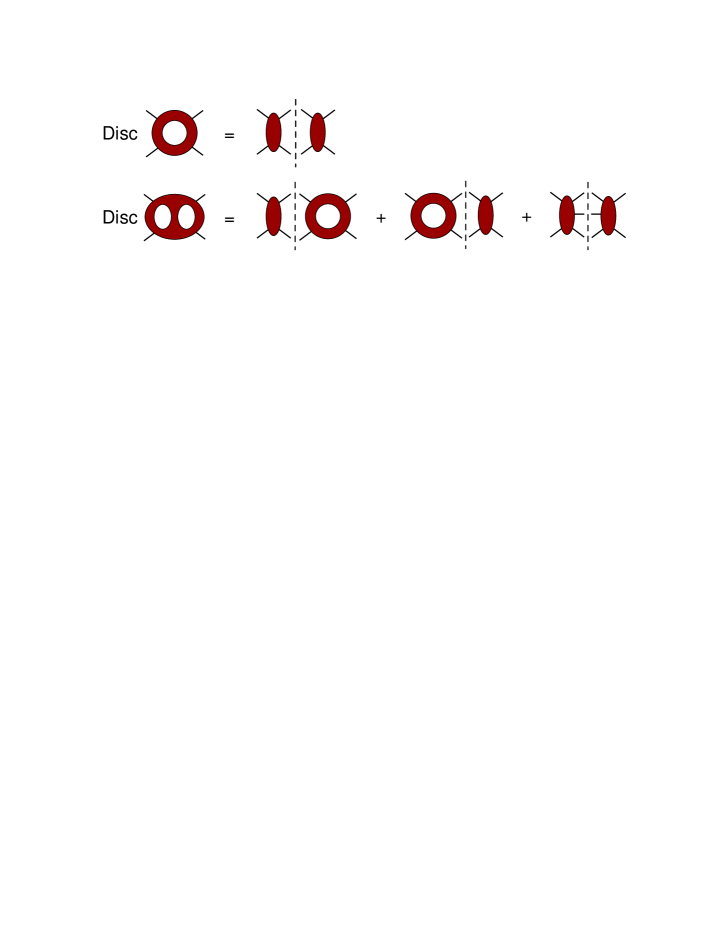
Figure 1: Unitarity relations for the four-point amplitude at one and two loops. The number of holes in a blob indicates the number of loops in the corresponding amplitude.

The scattering matrix is a unitary operator between in and out states: $S^{\dagger}S=1$, or in terms of the more standard “off-forward” scattering matrix, $T\equiv(S-1)/i$,

$$2\,\hbox{Disc}\,T=T^{\dagger}T\,,$$ (11)

where Disc $T\equiv(T-T^{\dagger})/2i$. This simple relation generates the well-known unitarity relations, or cutting rules Cutting , for the discontinuities (or absorptive parts) of perturbative amplitudes. If one inserts a perturbative expansion for $T$ into eq. (11), say

$$T_{4} = g^{2}\,T_{4}^{\rm tree}+g^{4}\,T_{4}^{\rm 1\hbox{-}loop}+g^{6}\,T_{4}^{\rm 2\hbox{-}loop}+\ldots\,,$$ (12)

$$T_{5} = g^{3}\,T_{5}^{\rm tree}+g^{5}\,T_{5}^{\rm 1\hbox{-}loop}+g^{7}\,T_{5}^{\rm 2\hbox{-}loop}+\ldots\,,$$ (13)

for the four- and five-point amplitudes, then one obtains the unitarity relations shown in Fig. 1.

At order $g^{4}$, the discontinuity in the one-loop four-point amplitude is given by the product of two order $g^{2}$ four-point tree amplitudes. The product must be summed over all possible intermediate states crossing the cut (indicated by the dashed line in Fig. 1), and integrated over all possible intermediate momenta. At two loops, or order $g^{6}$, there are two possible types of cuts: the product of a tree-level and a one-loop four-point amplitude ($g^{2}\times g^{4}$), and the product of two tree-level five-point amplitudes ($g^{3}\times g^{3}$).

To get the complete scattering amplitude, not just the absorptive part, one could try to reconstruct the real part via a dispersion relation. However, in the context of perturbation theory, an easier method is available, because one knows that the amplitude could have been calculated in terms of Feynman diagrams. Therefore it can be expressed as a linear combination of appropriate Feynman integrals, with coefficients that are rational functions of the kinematic variables. The unitarity method UnitarityMethod matches the information coming from the cuts against the set of available loop integrals in order to determine these rational coefficients. Using unitarity in $D=4-2\epsilon$ dimensions DDimUnitarity ; MultiLoopDDimGenUnitarity , one can also determine the so-called “rational terms”, which have no cuts in $D=4$.

Generalized unitarity GeneralizedUnitarityOld consists of imposing more than the minimal number of cut lines. It often simplifies enormously the information required to compute many terms in the amplitude ee4partons ; MoreGenUnitarity ; BCFUnitarity ; MultiLoopDDimGenUnitarity , especially in highly supersymmetric theories FourLoop ; GravityThree ; FiveLoop ; LeadingSingularity . Fig. 2 provides an example of generalized unitarity at the multi-loop level. One starts with an ordinary three-particle cut for a three-loop four-point amplitude. The information in this cut can be extracted more easily by cutting the one-loop five-point amplitude on the right-hand side of the cut, decomposing it into the product of a four-point tree and a five-point tree, in three inequivalent ways.

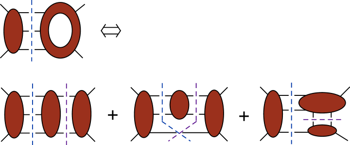
Figure 2: An example of multi-loop generalized unitarity. The one-loop five-point amplitude, appearing on the right side of the ordinary cut, is further cut into products of trees, in three inequivalent ways.

Fig. 2 illustrates a particular class of generalized unitarity cuts, in which all cut momenta are allowed to be real. It is possible, however, to impose more and more on-shell constraints on intermediate legs, dissolving the amplitude into products of more tree amplitudes, each with fewer legs (and hence simpler). For four-point amplitudes, the maximal cuts are the limiting cases in which all tree amplitudes are three-point ones, which can be dissolved no further. Fig. 3 shows how one of the real-momentum configurations in Fig. 2 generates several maximal cuts (which contain complex momenta). The method of maximal cuts FiveLoop ; CompactThree ; Neq44np ; CJtoappear for constructing a multi-loop amplitude begins with the evaluation of the maximal cuts, and the construction of a candidate ansatz for the loop-momentum integrand that is consistent with them. For simplicity we will discuss here the evaluation of four-dimensional cuts, that is, cuts in which the cut loop momenta are taken to be in four dimensions. For complete generality the cut loop momenta should be in $D$ dimensions. However, for the four-point amplitudes in maximally supersymmetric gauge theory or gravity, the $D$-dimensional cuts have yet to reveal any new terms, beyond those found using the four-dimensional cuts Neq44np .

For real momenta, the kinematics of the three-point process with all massless legs is singular — all three momenta must be parallel. However, for complex momenta it is perfectly nonsingular GoroffSagnotti ; WittenTwistor . The maximal cuts for four-point amplitudes are enumerated simply by drawing all cubic graphs. Their evaluation is also very simple, for four-dimensional cuts, because three-point tree amplitudes are always given by a simple expression in the usual spinor products, in either $\left\langle i\,j\right\rangle=\varepsilon_{\alpha\beta}\lambda_{i}^{\alpha}\lambda_{j}^{\beta}$ or $\left[i\,j\right]=\varepsilon_{\dot{\alpha}\dot{\beta}}\tilde{\lambda}_{i}^{\dot{\alpha}}\tilde{\lambda}_{j}^{\dot{\beta}}$, where $\lambda_{i}^{\alpha}$ ($\tilde{\lambda}_{i}^{\dot{\alpha}}$) is the two-component positive-chirality (negative-chirality) spinor associated with the massless momentum $k_{i}$. For example, for three gluons there are only two non-vanishing amplitudes,

$$A_{3}^{\rm tree}(1^{-},2^{-},3^{+})=i\,{{\left\langle 1\,2\right\rangle}^{4}\over\left\langle 1\,2\right\rangle\left\langle 2\,3\right\rangle\left\langle 3\,1\right\rangle}\,,\qquad A_{3}^{\rm tree}(1^{+},2^{+},3^{-})=-i\,{{\left[1\,2\right]}^{4}\over\left[1\,2\right]\left[2\,3\right]\left[3\,1\right]}\,.$$ (14)

There are two types of three-point complex kinematics; for each type, one of the two amplitudes in eq. (14) is non-vanishing and the other one vanishes WittenTwistor ; BCFUnitarity . Three-point amplitudes for gravity can be obtained directly as products of two gauge amplitudes, using eq. (7).

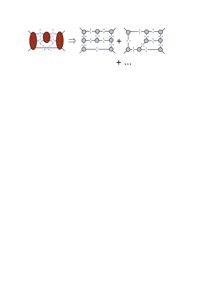
Figure 3: A generalized cut with real momenta generates several maximal cuts; the latter contain only three-point tree amplitudes.

Even though the maximal cuts are very simple to evaluate analytically, they provide a great deal of information, and an ansatz that satisfies the maximal cuts is an excellent starting point for constructing the full answer. For example, for the contributions to four-gluon scattering in ${{\cal N}=4}$ sYM that are planar (the dominant terms in the large $N_{c}$ limit), the maximal cuts find all terms present in the amplitude at one, two and three loops. They only start to miss planar terms at four loops (and non-planar terms at three loops). The remaining terms, whether planar or non-planar, can be found systematically by collapsing one propagator in each maximal cut to generate the next-to-maximal cuts; one more propagator to generate the next-to-next-to-maximal cuts; and so on. At each stage the ansatz is improved by adding more terms in order to fit the new information. Each additional term should contain at least one power of an inverse (collapsed) propagator $\ell_{i}^{2}$, corresponding to the fact that it was invisible on the maximal cut ($\ell_{i}^{2}=0$), and only became visible on the next-to-maximal cut ($\ell_{i}^{2}\neq 0$). The process of amplitude construction terminates when no more terms need to be added. Then the amplitude can be checked, by a comparison (usually numerical) against a complete, or “spanning” Neq44np , set of unitarity cuts.

VI Combining unitarity with KLT

The general strategy BDDPR we have adopted for computing multi-loop ${{\cal N}=8}$ supergravity amplitudes is to first compute the loop-momentum integrands for the corresponding amplitudes in ${{\cal N}=4}$ sYM. The integrands are described by a sum of Feynman integrals for cubic graphs, with standard scalar propagator factors and additional numerator polynomials. In the four-point case, the $p^{\rm th}$ such integral has the form,

$${\cal I}^{(p),\,{{\cal N}=4}\ {\rm sYM}}=C^{(p)}\times(-i)^{L}\int\biggl{(}\prod_{j=1}^{L}\frac{d^{D}\ell_{j}}{(2\pi)^{D}}\biggr{)}\,\frac{N^{(p)}(\ell_{j},k_{m})}{\prod_{n=1}^{3L+1}l_{n}^{2}}\,,$$ (15)

where $k_{m}$, $m=1,2,3$, are the three independent external momenta, $\ell_{j}$ are the $L$ independent loop momenta, and $l_{n}$ are the momenta of the $(3L+1)$ propagators (internal lines of the graph $p$), which are linear combinations of the $\ell_{j}$ and the $k_{m}$. As usual, $d^{D}\ell_{j}$ is the $D$-dimensional measure for the $j^{\rm th}$ loop momentum. The numerator polynomial $N^{(p)}(\ell_{j},k_{m})$ is a polynomial in both internal and external momenta. The color factor $C^{(p)}$ can be written as a product of structure constants $f^{abc}$ for the gauge group. It can also be written diagrammatically, using three-vertices for $f^{abc}$ factors, and lines (propagators) for $\delta^{ab}$ contractions. In this form, it is given just by the associated cubic graph.

These integrands can then be cut in any desired fashion. Through the KLT relations, they provide the data needed to evaluate very efficiently the generalized cuts for ${{\cal N}=8}$ supergravity. In particular, the ${{\cal N}=8}$ supergravity cuts require a sum over the 256 states in the ${{\cal N}=8}$ supergravity multiplet, for every cut line. However, the corresponding cut ${{\cal N}=4}$ sYM loop integrands already contain a sum over the 16 states in the ${{\cal N}=4}$ sYM multiplet. The KLT relations express the ${{\cal N}=8}$ supergravity cuts as sums of products of two copies of ${{\cal N}=4}$ sYM cuts. The ${{\cal N}=8}$ sum factorizes as,

$$\sum_{{{\cal N}=8}}\ =\ \sum_{[{{\cal N}=4}]_{L}}\sum_{[{{\cal N}=4}]_{R}}\ ,$$ (16)

and the ${{\cal N}=4}$ sums have already been carried out in the course of constructing the ${{\cal N}=4}$ sYM integrand.

Because gravity has no notion of color, planar and non-planar contributions cannot be separated in graviton amplitudes. The KLT relations therefore must relate the gravity cuts to both planar and non-planar gauge theory cuts. In other words, the complete ${{\cal N}=4}$ sYM amplitude, both planar (large $N_{c}$) and non-planar terms, is required in this method.

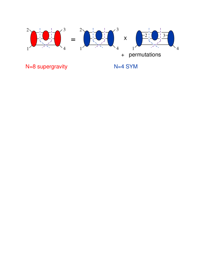
Figure 4: Evaluation of a generalized cut in ${{\cal N}=8}$ supergravity at three loops, in terms of planar and non-planar cuts in ${{\cal N}=4}$ sYM.

Fig. 4 sketches how the method works for a particular generalized cut at three loops. The ${{\cal N}=8}$ supergravity cut contains one four-point tree amplitude and two five-point ones. We use the KLT relations (8) and (9). We relabel them, and use the fact that $s_{12}s_{23}A_{4}^{\rm tree}(1,2,3,4)$ is totally symmetric in legs 1​,2,3,4 to rewrite them as,

$$M_{4}^{\rm tree}(\ell_{1},\ell_{2},\ell_{3},\ell_{4}) = -i{s_{\ell_{1}\ell_{2}}s_{\ell_{2}\ell_{3}}\over s_{\ell_{1}\ell_{3}}}\,A_{4}^{\rm tree}(\ell_{1},\ell_{2},\ell_{3},\ell_{4})\,\tilde{A}_{4}^{\rm tree}(\ell_{1},\ell_{2},\ell_{3},\ell_{4})\,,$$ (17)

$$M_{5}^{\rm tree}(1,2,\ell_{2},\ell_{1},\ell_{5}) = -is_{\ell_{5}1}s_{2\ell_{2}}\,A_{5}^{\rm tree}(1,2,\ell_{2},\ell_{1},\ell_{5})\,\tilde{A}_{5}^{\rm tree}(1,\ell_{1},2,\ell_{2},\ell_{5})\,+\,\mathcal{P}(1,2)\,,$$

$$M_{5}^{\rm tree}(4,3,\ell_{3},\ell_{4},\ell_{5}) = -is_{\ell_{5}4}s_{3\ell_{3}}\,A_{5}^{\rm tree}(4,3,\ell_{3},\ell_{4},\ell_{5})\,\tilde{A}_{5}^{\rm tree}(4,\ell_{4},3,\ell_{3},\ell_{5})\,+\,\mathcal{P}(3,4)\,.$$

In this way, both occurrences of the four-point ${{\cal N}=4}$ sYM amplitude carry the same cyclic ordering as the ${{\cal N}=8}$ supergravity one, as shown in the figure. One of the two five-point amplitudes carries the same ordering, as shown in the left copy. This copy can be evaluated using the planar ${{\cal N}=4}$ sYM amplitude. The other five-point amplitude is twisted, leading to the right copy, which is non-planar, so it requires non-planar terms in the ${{\cal N}=4}$ sYM amplitude. A reflection symmetry under the permutation $(1\leftrightarrow 4,\ 2\leftrightarrow 3)$ is preserved by this representation. The two-fold permutation sum in $M_{5}^{\rm tree}$ in eq. (17) leads to a four-fold permutation sum in the figure; one must add the permutations $(1\leftrightarrow 2)$, $(3\leftrightarrow 4)$, and $(1\leftrightarrow 2,\ 3\leftrightarrow 4)$.

Note that for terms that are detected in the maximal cuts, because of the simple relation between gravity and gauge three-point amplitudes (eq. (7)), the numerator factors are always simply squared in passing from gauge theory to gravity.

VII Explicit results

VII.1 Two loops

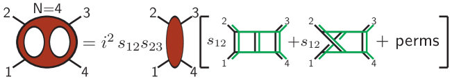
Figure 5: The two-loop amplitude in ${{\cal N}=4}$ sYM. The blob on the right represents the color-ordered tree amplitude $A_{4}^{\rm tree}$. In the brackets, black lines are kinematic $1/p^{2}$ propagators, with scalar ($\phi^{3}$) vertices. Green lines are color $\delta^{ab}$ propagators, with structure constant ($f^{abc}$) vertices.

The full two-loop four-point amplitude in ${{\cal N}=4}$ sYM is given by BRY ; BDDPR

$$A_{4}^{\rm 2\hbox{-}loop} = -s_{12}s_{23}A_{4}^{\rm tree}\Bigl{[}C^{{\rm P}}_{1234}\,s_{12}\,{\cal I}_{4}^{{\rm 2\hbox{-}loop},{\rm P}}(s_{12},s_{23})+C^{{\rm NP}}_{1234}\,s_{12}\,{\cal I}_{4}^{{\rm 2\hbox{-}loop},{\rm NP}}(s_{12},s_{23})$$ (18)

$$\hskip 65.44142pt\hbox{}+\mathcal{P}(2,3,4)\Bigr{]}\,,$$

where ${\cal I}_{4}^{{\rm 2\hbox{-}loop},({\rm P},{\rm NP})}$ are the scalar planar and non-planar double box integrals shown in Fig. 5, and $C^{({\rm P},{\rm NP})}_{1234}$ are color factors constructed from structure constant vertices, with the same graphical structure as the corresponding integral. The quantity $s_{12}s_{23}A_{4}^{\rm tree}$ is totally symmetric under gluon interchange, and its square is the $R^{4}$ matrix element in eq. (1), up to a factor of $i$. Because all terms in eq. (18) are detected by the maximal cuts, the complete two-loop four-point amplitude in ${{\cal N}=8}$ supergravity is found simply by squaring the prefactors in eq. (18) (and removing the color factors, as appropriate for gravity):

$$M_{4}^{\rm 2\hbox{-}loop} = -i(s_{12}s_{23}A_{4}^{\rm tree})^{2}\Bigl{[}s_{12}^{2}\,{\cal I}_{4}^{{\rm 2\hbox{-}loop},{\rm P}}(s_{12},s_{23})+s_{12}^{2}\,{\cal I}_{4}^{{\rm 2\hbox{-}loop},{\rm NP}}(s_{12},s_{23})+\mathcal{P}(2,3,4)\Bigr{]}$$

$$= s_{12}s_{23}s_{13}M_{4}^{\rm tree}\Bigl{[}s_{12}^{2}\,{\cal I}_{4}^{{\rm 2\hbox{-}loop},{\rm P}}(s_{12},s_{23})+s_{12}^{2}\,{\cal I}_{4}^{{\rm 2\hbox{-}loop},{\rm NP}}(s_{12},s_{23})+\mathcal{P}(2,3,4)\Bigr{]}\,.$$

(19)

Because the loop integrals appearing in the two amplitudes, eqs. (18) and (19), are precisely the same, the critical dimension $D_{c}$ is automatically the same for both theories at two loops. This value is $D_{c}=7$, the dimension in which the two-loop, seven-propagator integrals, $\sim\,\int d^{2D}\ell/(\ell^{2})^{7}$, are log divergent, in agreement with eqs. (2) and (3). The two-loop ${{\cal N}=8}$ supergravity divergence is associated with a counterterm of the form ${\cal D}^{4}R^{4}$ in $D=7$. This type of counterterm is permitted by the field-theoretic duality constraints of ref. Bossard2010bd .

VII.2 Three loops

At three loops, the integrand of the ${{\cal N}=4}$ sYM four-point amplitude begins to have dependence on the loop-momentum in its numerator, as well as (non-planar) terms that cannot be detected in the maximal cuts. For this reason, the three-loop ${{\cal N}=8}$ supergravity amplitude, in its initial two forms GravityThree ; CompactThree , was not given by simply squaring the ${{\cal N}=4}$ sYM results — except for a subset of the graphs that could be inferred using only two-particle cuts. More recently, three of the present authors rearranged the three-loop ${{\cal N}=4}$ sYM amplitude so as to make manifest its color-kinematic duality BCJ10 . In this form the ${{\cal N}=8}$ supergravity amplitude can once again be found by a simple squaring procedure. Here we will give the amplitudes in the form found in ref. CompactThree , which requires only the nine cubic graphs shown in Fig. 6. (Three more cubic graphs, containing three-point subdiagrams, enter the solution in ref. BCJ10 .)

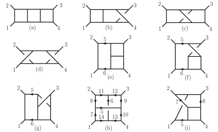
Figure 6: Cubic four-point graphs entering the four-point three-loop amplitudes.

Both the ${{\cal N}=4}$ sYM and ${{\cal N}=8}$ supergravity amplitudes are described by giving the loop-momentum numerator polynomials $N^{(p)}$ for these graphs. In addition, the ${{\cal N}=4}$ sYM graphs are multiplied by the corresponding color structure, as in Fig. 5.

Integral $I^{(p)}$	$N^{(p)}$ for ${{\cal N}=4}$ super-Yang-Mills
(a)–(d)	$s_{12}^{2}$
(e)–(g)	$s_{12}\,s_{46}$
(h)	$\;s_{12}(\tau_{26}+\tau_{36})+s_{23}(\tau_{15}+\tau_{25})+s_{12}s_{23}\;$
(i)	$\;s_{12}s_{45}-s_{23}s_{46}-{1\over 3}(s_{12}-s_{23})\ell_{7}^{2}\;$

Table 2: The numerator factors $N^{(p)}$ for the integrals $I^{(p)}$ in Fig. 6 for ${{\cal N}=4}$ super-Yang-Mills theory. The first column labels the integral, the second column the relative numerator factor. An overall factor of $s_{12}s_{23}A_{4}^{\rm tree}$ has been removed. The invariants $s_{ij}$ and $\tau_{ij}$ are defined in eq. (20).

Table 2 gives the values of $N^{(p)}$ for ${{\cal N}=4}$ sYM in terms of the following invariants,

$$s_{ij}=(k_{i}+k_{j})^{2}\,,\hskip 142.26378pt(i,j\leq 4)$$

$$s_{ij}=(k_{i}+\ell_{j})^{2}\,,\hskip 42.67912pt\tau_{ij}=2k_{i}\cdot\ell_{j}\,,\hskip 31.2982pt(i\leq 4,\ \ j\geq 5)$$

$$s_{ij}=(\ell_{i}+\ell_{j})^{2}\,.\hskip 145.10922pt(i,j\geq 5)$$ (20)

The external momenta $k_{i}$ are taken to be outgoing in Fig. 6; the directions of the loop momenta $\ell_{i}$ are indicated by arrows. Note that $s_{ij}$ is quadratic in the loop momenta $\ell_{i}$, if $j>4$, but $\tau_{ij}$ is linear. Every $N^{(p)}$ in Table 2 is manifestly quadratic (or better) in the loop momenta.

Integral $I^{(p)}$	$N^{(p)}$ for ${{\cal N}=8}$ supergravity
(a)–(d)	$\vphantom{\Bigr{|}}[s_{12}^{2}]^{2}$
(e)–(g)	$\vphantom{\Bigr{|}}s_{12}^{2}\,\tau_{35}\,\tau_{46}$
(h)	$\;(s_{12}(\tau_{26}+\tau_{36})+s_{23}(\tau_{15}+\tau_{25})+s_{12}s_{23})^{2}\;$
	$\;\hbox{}+(s_{12}^{2}(\tau_{26}+\tau_{36})-s_{23}^{2}(\tau_{15}+\tau_{25}))(\tau_{17}+\tau_{28}+\tau_{39}+\tau_{4,10})\;$
	$\;\hbox{}+s_{12}^{2}(\tau_{17}\tau_{28}+\tau_{39}\tau_{4,10})+s_{23}^{2}(\tau_{28}\tau_{39}+\tau_{17}\tau_{4,10})+s_{13}^{2}(\tau_{17}\tau_{39}+\tau_{28}\tau_{4,10})\;\vphantom{\Bigl{(}\Bigr{)}_{A_{A}}}$
(i)	$\vphantom{\bigl{|}_{A_{A}}}(s_{12}\,\tau_{45}-s_{23}\,\tau_{46})^{2}-\tau_{27}(s_{12}^{2}\,\tau_{45}+s_{23}^{2}\,\tau_{46})-\tau_{15}(s_{12}^{2}\,\tau_{47}+s_{13}^{2}\,\tau_{46})\;$
	$\;\hbox{}-\tau_{36}(s_{23}^{2}\,\tau_{47}+s_{13}^{2}\,\tau_{45})+\ell_{5}^{2}\,s_{12}^{2}\,s_{23}+\ell_{6}^{2}\,s_{12}\,s_{23}^{2}-{1\over 3}\ell_{7}^{2}\,s_{12}\,s_{13}\,s_{23}\;$

Table 3: Numerator factors $N^{(p)}$ for ${{\cal N}=8}$ supergravity. The first column labels the integral, the second column the relative numerator factor. An overall factor of $s_{12}s_{13}s_{14}M_{4}^{\rm tree}$ has been removed.

Table 3 gives the values of $N^{(p)}$ for ${{\cal N}=8}$ supergravity, in a form CompactThree which is also manifestly quadratic in the loop momenta. (In the first version of the amplitude GravityThree , the quadratic nature was not yet manifest.) Comparing the two sets of numerators, we see that the ${{\cal N}=8}$ supergravity ones are the squares of the ${{\cal N}=4}$ sYM ones, up to contact terms, as expected from the KLT relations. For example, in graphs (e)–(g), $s_{46}=\tau_{46}+\ell_{6}^{2}=\tau_{35}+\ell_{5}^{2}$, so $s_{12}^{2}\tau_{35}\tau_{46}\approx[s_{12}s_{46}]^{2}$ (modulo $\ell_{i}^{2}$ terms).

Because the numerator factors for both ${{\cal N}=8}$ supergravity and ${{\cal N}=4}$ sYM are manifestly quadratic in the loop momenta, the critical dimensions $D_{c}(L)$ at three loops remain equal, $D_{c}(L)=4+6/L=6$ for $L=3$. Indeed, when the ultraviolet poles in the integrals for ${{\cal N}=8}$ supergravity are evaluated, no further cancellation is found, and the resulting pole is

$$M_{4}^{{\rm 3\hbox{-}loop},\ D=6-2\epsilon}\bigr{|}_{\rm pole}\,=\,\frac{1}{\epsilon}\,{5\,\zeta_{3}\over(4\pi)^{9}}\,(s_{12}s_{23}s_{13})^{2}M_{4}^{\rm tree}\,,\hskip 8.5359pt$$ (21)

corresponding to a counterterm of the form ${\cal D}^{6}R^{4}$ in $D=6$. Again, the existence of this counterterm is consistent with the field-theoretic duality constraints of ref. Bossard2010bd .

The form of the divergence (21) was reproduced from string-theoretic duality arguments in ref. GRV2010 ; however, the rational number predicted there does not agree with eq. (21). Whether or not this indicates an issue in decoupling massive states from string theory to obtain ${{\cal N}=8}$ supergravity GOS remains unclear.

VII.3 Four Loops

Figure 7: Cubic vacuum graphs at four loops.

At four loops, the same general strategy still works, but the bookkeeping issues are greater Neq44np . One can start by classifying the cubic vacuum graphs. At three loops there were only two; at four loops there are five, shown in Fig. 7.

The next step is to decorate the five vacuum graphs with four external legs to get the cubic four-point graphs. As at lower loops, graphs containing triangles (three propagators or fewer on a loop) or other three point subgraphs can be dropped. (This statement would not be true for representations obeying the color-kinematic duality, as at three loops BCJ10 .) Fig. 7(a) only gives rise to triangle-containing graphs, so it can be dropped. Altogether there are 50 cubic four-point graphs with nonvanishing numerators. Graphs (b) and (c) do generate four-point graphs without triangles, but the numerators for all such graphs can be determined, up to possible contact terms, by iterated two-particle cuts. Because of the structure of these cuts BRY , the associated numerator polynomials turn out to be very simple. Graphs (d), and particularly (e), give rise to the most complex numerators.

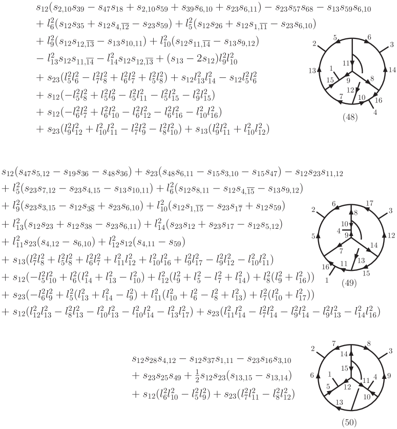
Figure 8: Integrals (48)-(50) for the four-loop ${{\cal N}=4}$ sYM amplitude Neq44np . The factor in front of each graph is the numerator polynomial $N^{(p)}$ for the integral $I^{(p)}$, where $(p)$ is the label below the graph. The kinematic variables are defined as $s_{ij}=s_{i,j}=(l_{i}+l_{j})^{2}$ and $s_{i,\overline{j}}=(l_{i}-l_{j})^{2}$, where $l_{i}$ is the momentum of line $i$.

The method of maximal cuts was used to determine the numerator polynomials for ${{\cal N}=4}$ sYM. At four loops, the maximal cuts have 13 cut conditions $\ell_{i}^{2}=0$. Then near-maximal cuts with only 12 cut conditions are considered, followed by ones with 11 cut conditions. At this point the ${{\cal N}=4}$ sYM ansatz is complete; no more terms need to be added. The result was verified by comparison against a spanning set of generalized cuts.

In Fig. 8 we show three of the 50 numerator polynomials. These three are associated with the one non-planar cubic vacuum graph (e), and they have the most complex numerators. Integral (50) is required for the ansatz for the integrand to match various cuts. However, it integrates to zero and has vanishing color factor, so it does not contribute to the ${{\cal N}=4}$ sYM amplitude. In constructing the amplitude, it proved very useful to have simple pictorial rules that allow one to generate numerator polynomials for many graphs from those for other graphs, either at the same loop order or at lower loop order. An old rule BRY , called the rung rule, applies whenever a graph has a two-particle cut. A newer rule is the box cut rule FiveLoop ; Neq44np . It can be applied to any graph that contains a four-point subdiagram, and it generates that graph’s numerator polynomial (modulo certain contact terms) from the polynomials associated with particular lower-loop graphs. Together, these rules are quite powerful; of the 50 graphs, only four have neither two-particle cuts nor box cuts. (Three of the four appear in Fig. 8.)

After the ${{\cal N}=4}$ sYM amplitude was computed, the 50 numerator polynomials for the ${{\cal N}=8}$ supergravity amplitude were then constructed, using information provided by the KLT relations. The results are quite lengthy, but are provided as Mathematica readable files in ref. Neq84 , along with some tools for manipulating them.

From the numerator polynomials for the ${{\cal N}=8}$ supergravity amplitude, the amplitude’s ultraviolet behavior could be extracted, by expanding the integrals in the limit of small external momenta, relative to the loop momenta TaylorExpand . Unlike the three-loop representations in refs. CompactThree ; BCJ10 , the ultraviolet behavior for the form in ref. Neq84 is not manifest. That means that each integral is more divergent than the sum, and hence subleading terms in the expansion are required. It is necessary to expand to third order, in order to show that ${{\cal N}=8}$ supergravity is as well behaved as ${{\cal N}=4}$ sYM at four loops, in this representation of the amplitude. More concretely, the numerator polynomials, omitting an overall factor of $stuM_{4}^{\rm tree}$, have a mass dimension of 12, i.e. each term is of the form $k^{12-m}\ell^{m}$, where $k$ and $\ell$ stand respectively for external and loop momenta. The maximum value of $m$ turns out to be 8 for every integral. The integrals all have 13 propagators, so they have the form ${\cal I}\sim\int d^{4D}\ell\,\ell^{8-26}$. The amplitude is manifestly finite in $D=4$, because $4\times 4+8-26<0$. (This result is not unexpected, given the absence of a ${\cal D}^{2}R^{4}$ counterterm DHHK ; Kallosh4loop .) The amplitude is not manifestly finite in $D=5$; to see that requires cancellation of the $k^{4}\ell^{8}$, $k^{5}\ell^{7}$ and $k^{6}\ell^{6}$ terms, after expansion around small $k$.

The cancellation of the $k^{4}\ell^{8}$ terms is relatively simple, because one can simply set the external momenta $k_{i}$ to zero inside the integrals that appear. At this point, the potentially divergent integrals all reduce to one of two types of scalar vacuum integrals — there are no loop-momentum tensors appearing in the numerator, and no doubled propagator factors in the denominator. In fact, only two of the five vacuum graphs in Fig. 7 appear, (d) and (e). Collecting all terms, one finds that the coefficients of (d) and (e) both vanish. The cancellation of the $k^{5}\ell^{7}$ terms (and the $k^{7}\ell^{5}$ terms) is trivial: Using dimensional regularization, with no dimensionful parameter, Lorentz invariance does not allow an odd-power divergence. The most intricate cancellation is that of the $k^{6}\ell^{6}$ terms, corresponding to the vanishing of the coefficient of the potential counterterm ${\cal D}^{6}R^{4}$ in $D=5$. In the expansion of the integrals to the second subleading order as $k_{i}\to 0$, thirty different four-loop vacuum integrals are generated. These integrals often have doubled (and sometimes tripled) propagators, arising from the Taylor expansion of the loop-momentum integrand in the external momentum. Some integrals also contain tensors in the loop-momentum in their numerators. However, there are consistency relations between the integrals, corresponding to the ability to shift the loop momenta by external momenta before expanding around $k_{i}=0$. These consistency relations are powerful enough to imply the cancellation of the ultraviolet pole in $D=5-2\epsilon$. As a check, we evaluated all 30 ultraviolet poles directly, with the same conclusion. We did not yet evaluate the ultraviolet pole near $D=11/2=5.5$ (the critical dimension for ${{\cal N}=4}$ sYM at this loop order), so in principle it could cancel, although that seems unlikely to be the case.

In summary, the four-loop four-point amplitude of ${{\cal N}=8}$ supergravity is ultraviolet finite for $D<11/2$ Neq84 , the same bound found for ${{\cal N}=4}$ super-Yang-Mills theory. Finiteness in $5\leq D<11/2$ is a consequence of nontrivial cancellations, beyond those already found at three loops GravityThree ; CompactThree . These results provide the strongest direct support to date for the possibility that ${{\cal N}=8}$ supergravity might be a perturbatively finite quantum theory of gravity.

VIII Conclusions

In every explicit computation to date, through four loops, the ultraviolet behavior of ${{\cal N}=8}$ supergravity has proven to be no worse than that of ${{\cal N}=4}$ super-Yang-Mills theory. On the other hand, there are several recent arguments Beisert2010jx ; Bossard2010bd in favor of the existence of a seven-loop counterterm Howe1980th of the form ${\cal D}^{8}R^{4}$. As argued in Section III, the five-loop four-graviton scattering amplitude, when evaluated in higher dimensions for the loop momentum, should provide a fairly decisive test for what will happen at seven loops. Although this computation is difficult, it may well prove feasible using new ideas related to the color-kinematic duality BCJ08 ; BCJ10 ; BDHK10 ; CJtoappear ; BCDJRtoappear .

Suppose that ${{\cal N}=8}$ supergravity turns out to be finite to all orders in perturbation theory. This result still would not prove that it is a consistent theory of quantum gravity at the non-perturbative level. There are at least two reasons to think that it might need a non-perturbative ultraviolet completion:

1. The (likely) $L!$ or worse growth of the coefficients of the order $L$ terms in the perturbative expansion, which for fixed-angle scattering, would imply a non-convergent behavior $\sim L!\,(s/M_{\rm Pl}^{2})^{L}$.

2. The fact that the perturbative series seems to be $E_{7(7)}$ invariant, while the mass spectrum of black holes is non-invariant (see e.g. ref. BFK for recent discussions).

QED is an example of a perturbatively well-defined theory that needs an ultraviolet completion; it also has factorial growth in its perturbative coefficients, $\sim L!\,\alpha^{L}$, due to ultraviolet renormalons associated with the Landau pole. Yet for small values of $\alpha$ QED works extremely well: it predicts the anomalous magnetic moment of the electron to 10 digits of accuracy. Also, there are many pointlike non-perturbative ultraviolet completions for QED, namely asymptotically free grand unified theories. Are there any imaginable pointlike completions for ${{\cal N}=8}$ supergravity? Maybe the only completion is string theory; or maybe this cannot happen because of the impossibility of decoupling non-perturbative string states not present in ${{\cal N}=8}$ supergravity GOS .

Another question is whether ${{\cal N}=8}$ supergravity might point the way to other, more realistic finite (or well behaved) theories of quantum gravity, having less supersymmetry and (perhaps) chiral fermions. One step in this direction could be to examine the multi-loop behavior of theories that can be thought of as spontaneously broken gauged ${{\cal N}=8}$ supergravity Ferrara1979fu , which are known to have improved ultraviolet behavior at one loop Sezgin1981ac .

In any event, the excellent perturbative ultraviolet behavior of ${{\cal N}=8}$ supergravity has already provided many surprises. Although the theory may not itself be of direct phenomenological interest, perhaps it will some day lead to more realistic theories also having excellent ultraviolet behavior. As a “toy model” for a pointlike theory of quantum gravity, it has been extremely instructive, and further exploration will no doubt be fruitful as well.

References

- (1) B. de Wit and D. Z. Freedman, Nucl. Phys. B 130, 105 (1977).
- (2) E. Cremmer, B. Julia and J. Scherk, Phys. Lett. B 76, 409 (1978).
- (3) E. Cremmer and B. Julia, Phys. Lett. B 80, 48 (1978); Nucl. Phys. B 159, 141 (1979).
- (4) H. Kawai, D. C. Lewellen and S. H. H. Tye, Nucl. Phys. B 269, 1 (1986).
- (5) Z. Bern, J. J. M. Carrasco and H. Johansson, Phys. Rev. D 78, 085011 (2008) [0805.3993 [hep-ph]].
- (6) R. J. Eden, P. V. Landshoff, D. I. Olive and J. C. Polkinghorne, The Analytic S Matrix (Cambridge University Press, 1966).
- (7) Z. Bern, L. J. Dixon and D. A. Kosower, Nucl. Phys. B 513, 3 (1998) [hep-ph/9708239].
-
(8)
Z. Bern, L. J. Dixon and D. A. Kosower,
JHEP 0001, 027 (2000)
[hep-ph/0001001];
JHEP 0408, 012 (2004) [hep-ph/0404293]. - (9) Z. Bern, V. Del Duca, L. J. Dixon and D. A. Kosower, Phys. Rev. D 71, 045006 (2005) [hep-th/0410224].
- (10) R. Britto, F. Cachazo and B. Feng, Nucl. Phys. B 725, 275 (2005) [hep-th/0412103].
- (11) Z. Bern, L. J. Dixon, D. C. Dunbar, M. Perelstein and J. S. Rozowsky, Nucl. Phys. B 530, 401 (1998) [hep-th/9802162].
- (12) Z. Bern, J. J. Carrasco, L. J. Dixon, H. Johansson, D. A. Kosower and R. Roiban, Phys. Rev. Lett. 98, 161303 (2007) [hep-th/0702112].
- (13) Z. Bern, J. J. M. Carrasco, L. J. Dixon, H. Johansson and R. Roiban, Phys. Rev. D 78, 105019 (2008) [0808.4112 [hep-th]].
- (14) Z. Bern, J. J. Carrasco, L. J. Dixon, H. Johansson and R. Roiban, Phys. Rev. Lett. 103, 081301 (2009) [0905.2326 [hep-th]].
- (15) Z. Bern, J. J. Carrasco, L. J. Dixon, H. Johansson and R. Roiban, Phys. Rev. D82, 125040 (2010) [1008.3327 [hep-th]].
- (16) Z. Bern, Living Rev. Rel. 5, 5 (2002) [gr-qc/0206071].
- (17) Z. Bern, J. J. M. Carrasco and H. Johansson, 0902.3765 [hep-th].
- (18) L. J. Dixon, 1005.2703 [hep-th].
- (19) Z. Bern, J. J. M. Carrasco and H. Johansson, Nucl. Phys. Proc. Suppl. 205-206, 54 (2010) [1007.4297 [hep-th]].
-
(20)
S. Weinberg, in Understanding the Fundamental Constituents of
Matter, ed. A. Zichichi (Plenum Press, New York, 1977);
S. Weinberg, in General Relativity, eds. S. W. Hawking and W. Israel
(Cambridge University Press, 1979), p. 700;
M. Niedermaier and M. Reuter, Living Rev. Rel. 9, 5 (2006). - (21) P. Hořava, Phys. Rev. D 79, 084008 (2009) [0901.3775 [hep-th]].
- (22) G. ’t Hooft and M. J. G. Veltman, Annales Poincare Phys. Theor. A 20, 69 (1974).
- (23) M. T. Grisaru, Phys. Lett. B 66, 75 (1977).
- (24) S. Deser, J. H. Kay and K. S. Stelle, Phys. Rev. Lett. 38, 527 (1977).
- (25) E. Tomboulis, Phys. Lett. B 67, 417 (1977).
-
(26)
M. T. Grisaru, H. N. Pendleton and P. van Nieuwenhuizen,
Phys. Rev. D 15, 996 (1977);
M. T. Grisaru and H. N. Pendleton, Nucl. Phys. B 124, 81 (1977). - (27) P. van Nieuwenhuizen and J. A. M. Vermaseren, Phys. Lett. B 65, 263 (1976).
- (28) S. Ferrara and B. Zumino, Nucl. Phys. B 134, 301 (1978).
- (29) S. Deser and J. H. Kay, Phys. Lett. B 76, 400 (1978).
- (30) P. S. Howe and U. Lindström, Nucl. Phys. B 181, 487 (1981).
- (31) R. E. Kallosh, Phys. Lett. B 99, 122 (1981).
- (32) D. J. Gross and E. Witten, Nucl. Phys. B 277, 1 (1986).
- (33) H. Elvang, D. Z. Freedman and M. Kiermaier, JHEP 1011, 016 (2010) [1003.5018 [hep-th]].
- (34) Z. Bern, L. J. Dixon, M. Perelstein and J. S. Rozowsky, Nucl. Phys. B 546, 423 (1999) [hep-th/9811140].
- (35) H. Elvang, D. Z. Freedman and M. Kiermaier, JHEP 1010, 103 (2010) [0911.3169 [hep-th]].
- (36) J. M. Drummond, P. J. Heslop, P. S. Howe and S. F. Kerstan, JHEP 0308, 016 (2003) [hep-th/0305202].
- (37) R. Kallosh, JHEP 0909, 116 (2009) [0906.3495 [hep-th]].
- (38) M. Bianchi, H. Elvang and D. Z. Freedman, JHEP 0809, 063 (2008) [0805.0757 [hep-th]].
- (39) N. Arkani-Hamed, F. Cachazo and J. Kaplan, JHEP 1009, 016 (2010) [0808.1446 [hep-th]].
- (40) R. Kallosh and T. Kugo, JHEP 0901, 072 (2009) [0811.3414 [hep-th]].
- (41) N. Marcus, Phys. Lett. B 157, 383 (1985).
- (42) G. Bossard, C. Hillmann and H. Nicolai, JHEP 1012, 052 (2010) [1007.5472 [hep-th]]
- (43) J. Brödel and L. J. Dixon, JHEP 1005, 003 (2010) [0911.5704 [hep-th]].
- (44) H. Elvang and M. Kiermaier, JHEP 1010, 108 (2010) [1007.4813 [hep-th]].
- (45) N. Beisert et al., Phys. Lett. B 694, 265 (2010) [1009.1643 [hep-th]].
- (46) D. Z. Freedman and E. Tonni, 1101.1672 [hep-th].
- (47) G. Bossard, P. S. Howe and K. S. Stelle, JHEP 1101, 020 (2011) [1009.0743 [hep-th]].
- (48) G. Bossard, P. S. Howe, K. S. Stelle, Phys. Lett. B 682, 137 (2009) [0908.3883 [hep-th]].
- (49) R. Kallosh, JHEP 1012, 009 (2010) [1009.1135 [hep-th]].
-
(50)
S. Mandelstam,
Nucl. Phys. B 213, 149 (1983);
P. S. Howe, K. S. Stelle and P. K. Townsend, Nucl. Phys. B 214, 519 (1983);
L. Brink, O. Lindgren and B. E. W. Nilsson, Phys. Lett. B 123, 323 (1983). - (51) J. Björnsson and M. B. Green, JHEP 1008, 132 (2010) [1004.2692 [hep-th]].
- (52) J. Björnsson, JHEP 1101, 002 (2011) [1009.5906 [hep-th]].
- (53) M. B. Green, J. H. Schwarz and L. Brink, Nucl. Phys. B 198, 474 (1982).
-
(54)
J. M. Drummond, M. Spradlin, A. Volovich and C. Wen,
Phys. Rev. D 79, 105018 (2009)
[0901.2363 [hep-th]];
N. E. J. Bjerrum-Bohr, P. H. Damgaard, B. Feng and T. Sondergaard, Phys. Rev. D 82, 107702 (2010) [1005.4367 [hep-th]; JHEP 1009, 067 (2010) [1007.3111 [hep-th]];
B. Feng and S. He, JHEP 1009, 043 (2010) [1007.0055 [hep-th]];
B. Feng, S. He, R. Huang and Y. Jia, JHEP 1010, 109 (2010) [1008.1626 [hep-th]];
N. E. J. Bjerrum-Bohr, P. H. Damgaard, T. Sondergaard and P. Vanhove, JHEP 1101, 001 (2011) [1010.3933 [hep-th]]. - (55) Z. Bern, T. Dennen, Y. t. Huang and M. Kiermaier, Phys. Rev. D 82, 065003 (2010) [1004.0693 [hep-th]]
- (56) Z. Bern, J. J. M. Carrasco and H. Johansson, Phys. Rev. Lett. 105, 061602 (2010) [1004.0476 [hep-th]].
- (57) J. J. M. Carrasco and H. Johansson, to appear.
- (58) Z. Bern, J. J. M. Carrasco, L. J. Dixon, H. Johansson and R. Roiban, to appear.
- (59) L. J. Dixon, in QCD & Beyond: Proceedings of TASI ’95, ed. D. E. Soper (World Scientific, 1996) [hep-ph/9601359].
-
(60)
L. D. Landau,
Nucl. Phys. 13, 181 (1959);
S. Mandelstam, Phys. Rev. 115, 1741 (1959);
R. E. Cutkosky, J. Math. Phys. 1, 429 (1960). - (61) Z. Bern, L. J. Dixon, D. C. Dunbar and D. A. Kosower, Nucl. Phys. B 425, 217 (1994) [hep-ph/9403226]; Nucl. Phys. B 435, 59 (1995) [hep-ph/9409265].
-
(62)
Z. Bern and A. G. Morgan,
Nucl. Phys. B 467, 479 (1996)
[hep-ph/9511336];
Z. Bern, L. J. Dixon, D. C. Dunbar and D. A. Kosower, Phys. Lett. B 394, 105 (1997) [hep-th/9611127]. - (63) Z. Bern, M. Czakon, L. J. Dixon, D. A. Kosower and V. A. Smirnov, Phys. Rev. D 75, 085010 (2007) [hep-th/0610248].
- (64) Z. Bern, J. J. M. Carrasco, H. Johansson and D. A. Kosower, Phys. Rev. D 76, 125020 (2007) [0705.1864 [hep-th]].
-
(65)
E. I. Buchbinder and F. Cachazo,
JHEP 0511, 036 (2005)
[hep-th/0506126];
F. Cachazo and D. Skinner, 0801.4574 [hep-th];
F. Cachazo, 0803.1988 [hep-th];
F. Cachazo, M. Spradlin and A. Volovich, Phys. Rev. D 78, 105022 (2008) [0805.4832 [hep-th]];
M. Spradlin, A. Volovich and C. Wen, Phys. Rev. D 78, 085025 (2008) [0808.1054 [hep-th]]. - (66) M. H. Goroff and A. Sagnotti, Phys. Lett. B 160, 81 (1985); Nucl. Phys. B 266, 709 (1986).
- (67) E. Witten, Commun. Math. Phys. 252, 189 (2004) [hep-th/0312171].
- (68) Z. Bern, J. S. Rozowsky and B. Yan, Phys. Lett. B 401, 273 (1997) [hep-ph/9702424].
- (69) M. B. Green, J. G. Russo and P. Vanhove, JHEP 1006, 075 (2010) [1002.3805 [hep-th]].
- (70) M. B. Green, H. Ooguri and J. H. Schwarz, Phys. Rev. Lett. 99, 041601 (2007) [0704.0777 [hep-th]].
-
(71)
A. A. Vladimirov,
Theor. Math. Phys. 43, 417 (1980)
[Teor. Mat. Fiz. 43, 210 (1980)];
N. Marcus and A. Sagnotti, Nuovo Cim. A 87, 1 (1985). - (72) M. Bianchi, S. Ferrara and R. Kallosh, Phys. Lett. B 690, 328 (2010) [0910.3674 [hep-th]]; JHEP 1003, 081 (2010) [0912.0057 [hep-th]].
- (73) S. Ferrara and B. Zumino, Phys. Lett. B 86, 279 (1979).
- (74) E. Sezgin and P. van Nieuwenhuizen, Nucl. Phys. B 195, 325 (1982).
-
(75)
D. Binosi and L. Theussl,
Comput. Phys. Commun. 161, 76 (2004)
[hep-ph/0309015];
D. Binosi, J. Collins, C. Kaufhold and L. Theussl, Comput. Phys. Commun. 180, 1709 (2009) [0811.4113 [hep-ph]]. - (76) J. A. M. Vermaseren, Comput. Phys. Commun. 83, 45 (1994).