Planning Graph Heuristics for Belief Space Search

Abstract

Some recent works in conditional planning have proposed reachability heuristics to improve planner scalability, but many lack a formal description of the properties of their distance estimates. To place previous work in context and extend work on heuristics for conditional planning, we provide a formal basis for distance estimates between belief states. We give a definition for the distance between belief states that relies on aggregating underlying state distance measures. We give several techniques to aggregate state distances and their associated properties. Many existing heuristics exhibit a subset of the properties, but in order to provide a standardized comparison we present several generalizations of planning graph heuristics that are used in a single planner. We compliment our belief state distance estimate framework by also investigating efficient planning graph data structures that incorporate BDDs to compute the most effective heuristics.

We developed two planners to serve as test-beds for our investigation. The first, CAltAlt, is a conformant regression planner that uses A* search. The second, $POND$, is a conditional progression planner that uses AO* search. We show the relative effectiveness of our heuristic techniques within these planners. We also compare the performance of these planners with several state of the art approaches in conditional planning.

1 Introduction

Ever since CGP (?) and SGP (?) a series of planners have been developed for tackling conformant and conditional planning problems – including GPT (?), C-Plan (?), PKSPlan (?), Frag-Plan (?), MBP (?), KACMBP (?), CFF (?), and YKA (?). Several of these planners are extensions of heuristic state space planners that search in the space of “belief states” (where a belief state is a set of possible states). Without full-observability, agents need belief states to capture state uncertainty arising from starting in an uncertain state or by executing actions with uncertain effects in a known state. We focus on the first type of uncertainty, where an agent starts in an uncertain state but has deterministic actions. We seek strong plans, where the agent will reach the goal with certainty despite its partially known state. Many of the aforementioned planners find strong plans, and heuristic search planners are currently among the best. Yet a foundation for what constitutes a good distance-based heuristic for belief space has not been adequately investigated.

Belief Space Heuristics: Intuitively, it can be argued that the heuristic merit of a belief state depends on at least two factors–the size of the belief state (i.e., the uncertainty in the current state), and the distance of the individual states in the belief state from a destination belief state. The question of course is how to compute these measures and which are most effective. Many approaches estimate belief state distances in terms of individual state to state distances between states in two belief states, but either lack effective state to state distances or ways to aggregate the state distances. For instance the MBP planner (?) counts the number of states in the current belief state. This amounts to assuming each state distance has unit cost, and planning for each state can be done independently. The GPT planner (?) measures the state to state distances exactly and takes the maximum distance, assuming the states of the belief state positively interact.

Heuristic Computation Substrates: We characterize several approaches to estimating belief state distance by describing them in terms of underlying state to state distances. The basis of our investigation is in adapting classical planning reachability heuristics to measure state distances and developing state distance aggregation techniques to measure interaction between plans for states in a belief state. We take three fundamental approaches to measure the distance between two belief states. The first approach does not involve aggregating state distance measures, rather we use a classical planning graph to compute a representative state distance. The second retains distinctions between individual states in the belief state by using multiple planning graphs, akin to CGP (?), to compute many state distance measures which are then aggregated. The third employs a new planning graph generalization, called the Labelled Uncertainty Graph ($LUG$), that blends the first two to measure a single distance between two belief states. With each of these techniques we will discuss the types of heuristics that we can compute with special emphasis on relaxed plans. We present several relaxed plan heuristics that differ in terms of how they employ state distance aggregation to make stronger assumptions about how states in a belief state can co-achieve the goal through action sequences that are independent, positively interact, or negatively interact.

Our motivation for the first of the three planning graph techniques for measuring belief state distances is to try a minimal extension to classical planning heuristics to see if they will work for us. Noticing that our use of classical planning heuristics ignores distinctions between states in a belief state and may provide uninformed heuristics, we move to the second approach where we possibly build exponentially many planning graphs to get a better heuristic. With the multiple planning graphs we extract a heuristic from each graph and aggregate them to get the belief state distance measure. If we assume the states of a belief state are independent, we can aggregate the measures with a summation. Or, if we assume they positively interact we can use a maximization. However, as we will show, relaxed plans give us a unique opportunity to measure both positive interaction and independence among the states by essentially taking the union of several relaxed plans. Moreover, mutexes play a role in measuring negative interactions between states. Despite the utility of having robust ways to aggregate state distances, we are still faced with the exponential blow up in the number of planning graphs needed. Thus, our third approach seeks to retain the ability to measure the interaction of state distances but avoid computing multiple graphs and extracting heuristics from each. The idea is to condense and symbolically represent multiple planning graphs in a single planning graph, called a Labelled Uncertainty Graph ($LUG$). Loosely speaking, this single graph unions the causal support information present in the multiple graphs and pushes the disjunction, describing sets of possible worlds (i.e., initial literal layers), into “labels”. The planning graph vertices are the same as those present in multiple graphs, but redundant representation is avoided. For instance an action that was present in all of the multiple planning graphs would be present only once in the $LUG$ and labelled to indicate that it is applicable in a planning graph projection from each possible world. We will describe how to extract heuristics from the $LUG$ that make implicit assumptions about state interaction without explicitly aggregating several state distances.

Ideally, each of the planning graph techniques considers every state in a belief state to compute heuristics, but as belief states grow in size this could become uninformed or costly. For example, the single classical planning graph ignores distinctions between possible states where the heuristic based on multiple graphs leads to the construction of a planning graph for each state. One way to keep costs down is to base the heuristics on only a subset of the states in our belief state. We evaluate the effect of such a sampling on the cost of our heuristics. With a single graph we sample a single state and with multiple graphs and the $LUG$ we sample some percent of the states. We evaluate state sampling to show when it is appropriate, and find that it is dependent on how we compute heuristics with the states.

Standardized Evaluation of Heuristics: An issue in evaluating the effectiveness of heuristic techniques is the many architectural differences between planners that use the heuristics. It is quite hard to pinpoint the global effect of the assumptions underlying their heuristics on performance. For example, GPT is outperformed by MBP–but it is questionable as to whether the credit for this efficiency is attributable to the differences in heuristics, or differences in search engines (MBP uses a BDD-based search). Our interest in this paper is to systematically evaluate a spectrum of approaches for computing heuristics for belief space planning. Thus we have implemented heuristics similar to GPT and MBP and use them to compare against our new heuristics developed around the notion of overlap (multiple world positive interaction and independence). We implemented the heuristics within two planners, the Conformant-$AltAlt$ planner (${\cal C}{\sl AltAlt}$) and the Partially-Observable Non-Deterministic planner ($POND$). $POND$ does handle search with non-deterministic actions, but for the bulk of the paper we discuss deterministic actions. This more general action formulation, as pointed out by ? (?), can be translated into initial state uncertainty. Alternatively, in Section 8.2 we discuss a more direct approach to reason with non-deterministic actions in the heuristics.

External Evaluation: Although our main interest in this paper is to evaluate the relative advantages of a spectrum of belief space planning heuristics in a normalized setting, we also compare the performance of the best heuristics from this work to current state of the art conformant and conditional planners. Our empirical studies show that planning graph based heuristics provide effective guidance compared to cardinality heuristics as well as the reachability heuristic used by GPT and CFF, and our planners are competitive with BDD-based planners such as MBP and YKA, and GraphPlan-based ones such as CGP and SGP. We also notice that our planners gain scalability with our heuristics and retain reasonable quality solutions, unlike several of the planners we compare against.

The rest of this paper is organized as follows. We first present the ${\cal C}{\sl AltAlt}$ and $POND$ planners by describing their state and action representations as well as their search algorithms. To understand search guidance in the planners, we then discuss appropriate properties of heuristic measures for belief space planning. We follow with a description of the three planning graph substrates used to compute heuristics. We carry out an empirical evaluation in the next three sections, by describing our test setup, presenting a standardized internal comparison, and finally comparing with several other state of the art planners. We end with related research, discussion, prospects for future work, and various concluding remarks.

2 Belief Space Planners

Our planning formulation uses regression search to find strong conformant plans and progression search to find strong conformant and conditional plans. A strong plan guarantees that after a finite number of actions executed from any of the many possible initial states, all resulting states are goal states. Conformant plans are a special case where the plan has no conditional plan branches, as in classical planning. Conditional plans are a more general case where plans are structured as a graph because they include conditional actions (i.e. the actions have causative and observational effects). In this presentation, we restrict conditional plans to DAGs, but there is no conceptual reason why they cannot be general graphs. Our plan quality metric is the maximum plan path length.

We formulate search in the space of belief states, a technique described by ? (?). The planning problem $P$ is defined as the tuple $\langle D,BS_{I},BS_{G}\rangle$, where $D$ is a domain description, $BS_{I}$ is the initial belief state, and $BS_{G}$ is the goal belief state (consisting of all states satisfying the goal). The domain $D$ is a tuple $\langle F,A\rangle$, where $F$ is a set of fluents and $A$ is a set of actions.

Logical Formula Representation: We make extensive use of logical formulas over $F$ to represent belief states, actions, and $LUG$ labels, so we first explain a few conventions. We refer to every fluent in $F$ as either a positive literal or a negative literal, either of which is denoted by $l$. When discussing the literal $l$, the opposite polarity literal is denoted $\neg l$. Thus if $l$ = $\neg$at(location1), then $\neg l$ = at(location1). We reserve the symbols $\perp$ and $\top$ to denote logical false and true, respectively. Throughout the paper we define the conjunction of an empty set equivalent to $\top$, and the disjunction of an empty set as $\perp$.

Logical formulas are propositional sentences comprised of literals, disjunction, conjunction, and negation. We refer to the set of models of a formula $f$ as ${\cal M}(f)$. We consider the disjunctive normal form of a logical formula $f$, $\hat{\xi}(f)$, and the conjunctive normal form of $f$, $\kappa(f)$. The DNF is seen as a disjunction of “constituents” $\hat{S}$ each of which is a conjunction of literals. Alternatively the CNF is seen as a conjunction of “clauses” $C$ each of which is a disjunction of literals. We find it useful to think of DNF and CNF represented as sets – a disjunctive set of constituents or a conjunctive set of clauses. We also refer to the complete representation $\xi(f)$ of a formula $f$ as a DNF where every constituent – or in this case state $S$ – is a model of $f$.

Belief State Representation: A world state, $S$, is represented as a complete interpretation over fluents. We also refer to states as possible worlds. A belief state $BS$ is a set of states and is symbolically represented as a propositional formula over $F$. A state $S$ is in the set of states represented by a belief state $BS$ if $S\in{\cal M}(BS)$, or equivalently $S\models BS$.

For pedagogical purposes, we use the bomb and toilet with clogging and sensing problem, BTCS, as a running example for this paper. BTCS is a problem that includes two packages, one of which contains a bomb, and there is also a toilet in which we can dunk packages to defuse potential bombs. The goal is to disarm the bomb and the only allowable actions are dunking a package in the toilet (DunkP1, DunkP2), flushing the toilet after it becomes clogged from dunking (Flush), and using a metal-detector to sense if a package contains the bomb (DetectMetal). The fluents encoding the problem denote that the bomb is armed (arm) or not, the bomb is in a package (inP1, inP2) or not, and that the toilet is clogged (clog) or not. We also consider a conformant variation on BTCS, called BTC, where there is no DetectMetal action.

The belief state representation of the BTCS initial condition, in clausal representation is:

$\kappa(BS_{I})$ = arm $\wedge\neg$clog $\wedge$ (inP1 $\vee$ inP2) $\wedge$ ($\neg$inP1 $\vee\neg$inP2),

and in constituent representation is:

$\hat{\xi}(BS_{I})$ = (arm $\wedge\neg$ clog $\wedge$ inP1 $\wedge\neg$inP2) $\vee$ (arm $\wedge\neg$ clog $\wedge\neg$inP1 $\wedge$ inP2).

The goal of BTCS has the clausal and constituent representation:

$\kappa(BS_{G})$ = $\hat{\xi}(BS_{G})$ = $\neg$arm.

However, the goal has the complete representation:

$\xi(BS_{G})$ = ($\neg$arm $\wedge$ clog $\wedge$ inP1 $\wedge\neg$inP2) $\vee$ ($\neg$arm $\wedge$ clog $\wedge\neg$inP1 $\wedge$ inP2) $\vee$
                ($\neg$arm $\wedge\neg$clog $\wedge$ inP1 $\wedge\neg$inP2) $\vee$ ($\neg$arm $\wedge\neg$clog $\wedge\neg$inP1 $\wedge$ inP2) $\vee$
                ($\neg$arm $\wedge$ clog $\wedge\neg$inP1 $\wedge\neg$inP2) $\vee$ ($\neg$arm $\wedge$ clog $\wedge$ inP1 $\wedge$ inP2) $\vee$
                ($\neg$arm $\wedge\neg$clog $\wedge\neg$inP1 $\wedge\neg$inP2) $\vee$ ($\neg$arm $\wedge\neg$clog $\wedge$ inP1 $\wedge$ inP2).

The last four states (disjuncts) in the complete representation are unreachable, but consistent with the goal description.

Action Representation: We represent actions as having both causative and observational effects. All actions $a$ are described by a tuple $\langle\rho^{e}(a),\Phi(a),\Theta(a)\rangle$ where $\rho^{e}(a)$ is an execution precondition, $\Phi(a)$ is a set of causative effects, and $\Theta(a)$ is a set of observations. The execution precondition, $\rho^{e}(a)$, is a conjunction of literals that must hold for the action to be executable. If an action is executable, we apply the set of causative effects to find successor states and then apply the observations to partition the successor states into observational classes.

Each causative effect $\varphi^{j}(a)\in\Phi(a)$ is a conditional effect of the form $\rho^{j}(a)$$\implies$$\varepsilon^{j}(a)$, where the antecedent $\rho^{j}(a)$ and consequent $\varepsilon^{j}(a)$ are both a conjunction of literals. We handle disjunction in $\rho^{e}(a)$ or a $\rho^{j}(a)$ by replicating the respective action or effect with different conditions, so with out loss of generality we assume conjunctive preconditions. However, we cannot split disjunction in the effects. Disjunction in an effect amounts to representing a set of non-deterministic outcomes. Hence we do not allow disjunction in effects thereby restricting to deterministic effects. By convention $\varphi^{0}(a)$ is an unconditional effect, which is equivalent to a conditional effect where $\rho^{0}(a)=\top$.

The only way to obtain observations is to execute an action with observations. Each observation formula $o^{j}(a)\in\Theta(a)$ is a possible sensor reading. For example, an action $a$ that observes the truth values of two fluents $p$ and $q$ defines $\Theta(a)=\{p\wedge q,\neg p\wedge q,p\wedge\neg q,\neg p\wedge\neg q\}$. This differs slightly from the conventional description of observations in the conditional planning literature. Some works (e.g., ?) describe an observation as a list of observable formulas, then define possible sensor readings as all boolean combinations of the formulas. We directly define the possible sensor readings, as illustrated by our example. We note that our convention is helpful in problems where some boolean combinations of observable formulas will never be sensor readings.

The causative and sensory actions for the example BTCS problem are:

DunkP1: $\langle\rho^{e}$ = $\neg$clog, $\Phi=\{\varphi^{0}=$ clog, $\varphi^{1}=$ inP1 $\implies\neg$arm$\},\Theta=\{\}\rangle$,

DunkP2: $\langle\rho^{e}=\neg$clog, $\Phi=\{\varphi^{0}=$ clog, $\varphi^{1}=$ inP2 $\implies\neg$arm$\},\Theta=\{\}\rangle$,

Flush: $\langle\rho^{e}=\top$, $\Phi=\{\varphi^{0}=\neg$clog$\},\Theta=\{\}\rangle$, and

DetectMetal: $\langle\rho^{e}=\top,\Phi=\emptyset,\Theta=\{o^{0}=$ inP1, $o^{1}=\neg$inP1$\}\rangle$.

2.1 Regression

We perform regression in the CAltAlt planner to find conformant plans by starting with the goal belief state and regressing it non-deterministically over all relevant actions. An action (without observations) is relevant for regressing a belief state if (i) its unconditional effect is consistent with every state in the belief state and (ii) at least one effect consequent contains a literal that is present in a constituent of the belief state. The first part of relevance requires that every state in the successor belief state is actually reachable from the predecessor belief state and the second ensures that the action helps support the successor.

Following ? (?), regressing a belief state $BS$ over an action $a$, with conditional effects, involves finding the execution, causation, and preservation formulas. We define regression in terms of clausal representation, but it can be generalized for arbitrary formulas. The regression of a belief state is a conjunction of the regression of clauses in $\kappa(BS)$. Formally, the result $BS^{\prime}$ of regressing the belief state $BS$ over the action $a$ is defined as:

$$BS^{\prime}={\tt Regress}(BS,a)=\Pi(a)\wedge\left(\bigwedge_{C\in{\kappa(BS})}\;\bigvee_{l\in C}\left(\Sigma(a,l)\wedge IP(a,{l})\right)\right)$$

Execution formula ($\Pi({a})$) is the execution precondition $\rho^{e}(a)$. This is what must hold in $BS^{\prime}$ for $a$ to have been applicable.

Causation formula ($\Sigma(a,{l})$) for a literal $l$ w.r.t all effects $\varphi^{i}(a)$ of an action $a$ is defined as the weakest formula that must hold in the state before $a$ such that $l$ holds in $BS$. The intuitive meaning is that $l$ already held in $BS^{\prime}$, or the antecedent $\rho^{i}(a)$ must have held in $BS^{\prime}$ to make $l$ hold in $BS$. Formally $\Sigma(a,l)$ is defined as:

$$\Sigma(a,{l})=l\vee\bigvee_{\begin{subarray}{c}i:l\in\varepsilon^{i}(a)\end{subarray}}\rho^{i}(a)$$

Preservation formula ($IP(a,{l})$) of a literal $l$ w.r.t. all effects $\varphi^{i}(a)$ of action $a$ is defined as the formula that must be true before $a$ such that $l$ is not violated by any effect $\varepsilon^{i}(a)$. The intuitive meaning is that the antecedent of every effect that is inconsistent with $l$ could not have held in $BS^{\prime}$. Formally $IP(a,{l})$ is defined as:

$$IP(a,{l})=\bigwedge_{\begin{subarray}{c}i:\neg l\in\varepsilon^{i}(a)\end{subarray}}\neg\rho^{i}(a)$$

Regression has also been formalized in the MBP planner (?) as a symbolic pre-image computation of BDDs (?). While our formulation is syntactically different, both approaches compute the same result.

2.2 ${\cal C}{\sl AltAlt}$

The CAltAlt planner uses the regression operator to generate children in an A* search. Regression terminates when search node expansion generates a belief state $BS$ which is logically entailed by the initial belief state $BS_{I}$. The plan is the sequence of actions regressed from $BS_{G}$ to obtain the belief state entailed by $BS_{I}$.

For example, in the BTC problem, Figure 1, we have:

$BS_{2}=$Regress$(BS_{G},$ DunkP1) = $\neg$clog $\wedge$ ($\neg$arm $\vee$ inP1).

The first clause is the execution formula and the second clause is the causation formula for the conditional effect of DunkP1 and $\neg$arm.

Regressing $BS_{2}$ with Flush gives:

$BS_{4}=$ Regress$(BS_{2},$ Flush$)=$ ($\neg$arm $\vee$ inP1).

For $BS_{4}$, the execution precondition of Flush is $\top$, the causation formula is $\top\vee\neg$clog $=\top$, and ($\neg$arm $\vee$ inP1) comes by persistence of the causation formula.

Finally, regressing $BS_{4}$ with DunkP2 gives:

$BS_{9}=$ Regress$(BS_{4},$ DunkP2) = $\neg$clog $\wedge$ ($\neg$arm $\vee$ inP1 $\vee$ inP2).

We terminate at $BS_{9}$ because $BS_{I}\models BS_{9}$. The plan is DunkP2, Flush, DunkP1.

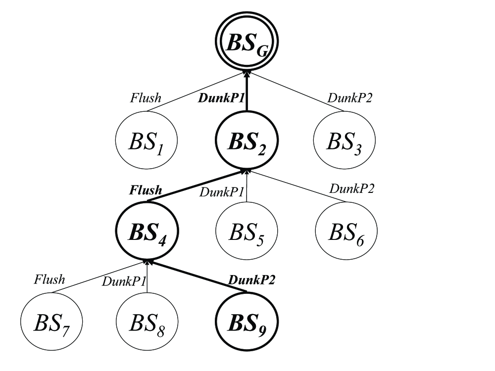
Figure 1: Illustration of the regression search path for a conformant plan in the $BTC$ problem.

2.3 Progression

In progression we can handle both causative effects and observations, so in general, progressing the action $a$ over the belief state $BS$ generates the set of successor belief states $B$. The set of belief states $B$ is empty when the action is not applicable to $BS$ ($BS\not\models\rho^{e}(a)$).

Progression of a belief state $BS$ over an action $a$ is best understood as the union of the result of applying $a$ to each model of $BS$ but we in fact implement it as BDD images, as in the MBP planner (?). Since we compute progression in two steps, first finding a causative successor, and second partitioning the successor into observational classes, we explain the steps separately. The causative successor $BS^{\prime}$ is found by progressing the belief state $BS$ over the causative effects of the action $a$. If the action is applicable, the causative successor is the disjunction of causative progression (Progress_c) for each state in $BS$ over $a$:

$$BS^{\prime}={\tt Progress}_{c}(BS,a)=\left\{\begin{array}[]{c @{\quad:\quad}l}\perp&BS\not\models\rho^{e}(a)\\ \bigvee\limits_{S\in{\cal M}(BS)}{\tt Progress}_{c}(S,a)&{\tt otherwise}\\ \end{array}\right.$$

The progression of an action $a$ over a state $S$ is the conjunction of every literal that persists (no applicable effect consequent contains the negation of the literal) and every literal that is given as an effect (an applicable effect consequent contains the literal).

$$S^{\prime}={\tt Progress}_{c}(S,a)=\bigwedge\limits_{\begin{subarray}{c}l:l\in S\;{\tt and}\\ \neg\exists_{j}\;S\models\rho^{j}(a)\;{\tt and}\\ \neg l\in\varepsilon^{j}(a)\end{subarray}}l\wedge\bigwedge\limits_{\begin{subarray}{c}l:\exists_{j}\;S\models\rho^{j}(a)\;{\tt and}\\ l\in\varepsilon^{j}(a)\end{subarray}}l$$

Applying the observations of an action results in the set of successors $B$. The set is found (in Progress_s) by individually taking the conjunction of each sensor reading $o^{j}(a)$ with the causative successor $BS^{\prime}$. Applying the observations $\Theta(a)$ to a belief state $BS^{\prime}$ results in a set $B$ of belief states, defined as:

$$B={\tt Progress}_{s}(BS^{\prime},a)=\left\{\begin{array}[]{l @{\quad:\quad}l}\perp&BS^{\prime}=\perp\\ \{BS^{\prime}\}&\Theta(a)=\emptyset\\ \{BS^{\prime\prime}|BS^{\prime\prime}=o^{j}(a)\wedge BS^{\prime}\}&{\tt otherwise}\\ \end{array}\right.\\$$

The full progression is computed as:

$B$ = Progress($BS,a$) = Progress${}_{s}($Progress${}_{c}(BS,a),a)$.

2.4 $POND$

We use top down AO* search (?), in the $POND$ planner to generate conformant and conditional plans. In the search graph, the nodes are belief states and the hyper-edges are actions. We need AO* because applying an action with observations to a belief state divides the belief state into observational classes. We use hyper-edges for actions because actions with observations have several possible successor belief states, all of which must be included in a solution.

The AO* search consists of two repeated steps: expand the current partial solution, and then revise the current partial solution. Search ends when every leaf node of the current solution is a belief state that satisfies the goal and no better solution exists (given our heuristic function). Expansion involves following the current solution to an unexpanded leaf node and generating its children. Revision is a dynamic programming update at each node in the current solution that selects a best hyper-edge (action). The update assigns the action with minimum cost to start the best solution rooted at the given node. The cost of a node is the cost of its best action plus the average cost of its children (the nodes connected through the best action). When expanding a leaf node, the children of all applied actions are given a heuristic value to indicate their estimated cost.

The main differences between our formulation of AO* and that of ? (?) are that we do not allow cycles in the search graph, we update the costs of nodes with an average rather than a summation, and use a weighted estimate of future cost. The first difference is to ensure that plans are strong (there are a finite number of steps to the goal), the second is to guide search toward plans with lower average path cost, and the third is to bias our search to trust the heuristic function. We define our plan quality metric (maximum plan path length) differently than the metric our search minimizes for two reasons. First, it is easier to compare to other competing planners because they measure the same plan quality metric. Second, search tends to be more efficient using the average instead of the maximum cost of an action’s children. By using average instead of maximum, the measured cost of a plan is lower – this means that we are likely to search a shallower search graph to prove a solution is not the best solution.

Conformant planning, using actions without observations, is a special case for AO* search, which is similar to A* search. The hyper-edges that represent actions are singletons, leading to a single successor belief state. Consider the BTC problem (BTCS without the DetectMetal action) with the future cost (heuristic value) set to zero for every search node. We show the search graph in Figure 2 for this conformant example as well as a conditional example, described shortly. We can expand the initial belief state by progressing it over all applicable actions. We get:

$B_{1}=\{BS_{10}\}=$ Progress($BS_{I},$ DunkP1)
      $=$ {(inP1 $\wedge\neg$inP2 $\wedge$ clog $\wedge\neg$arm) $\vee$ ($\neg$inP1 $\wedge$ inP2 $\wedge$ clog $\wedge$ arm)}

and

$B_{3}=\{BS_{20}\}=$ Progress($BS_{I},$ DunkP2)
      $=$ {(inP1 $\wedge\neg$inP2 $\wedge$ clog $\wedge$ arm) $\vee$ ($\neg$inP1 $\wedge$ inP2 $\wedge$ clog $\wedge\neg$arm)}.

Since $\neg$clog already holds in every state of the initial belief state, applying Flush to $BS_{I}$ leads to $BS_{I}$ creating a cycle. Hence, a hyper-edge for Flush is not added to the search graph for $BS_{I}$. We assign a cost of zero to $BS_{10}$ and $BS_{20}$, update the internal nodes of our best solution, and add DunkP1 to the best solution rooted at $BS_{I}$ (whose cost is now one).

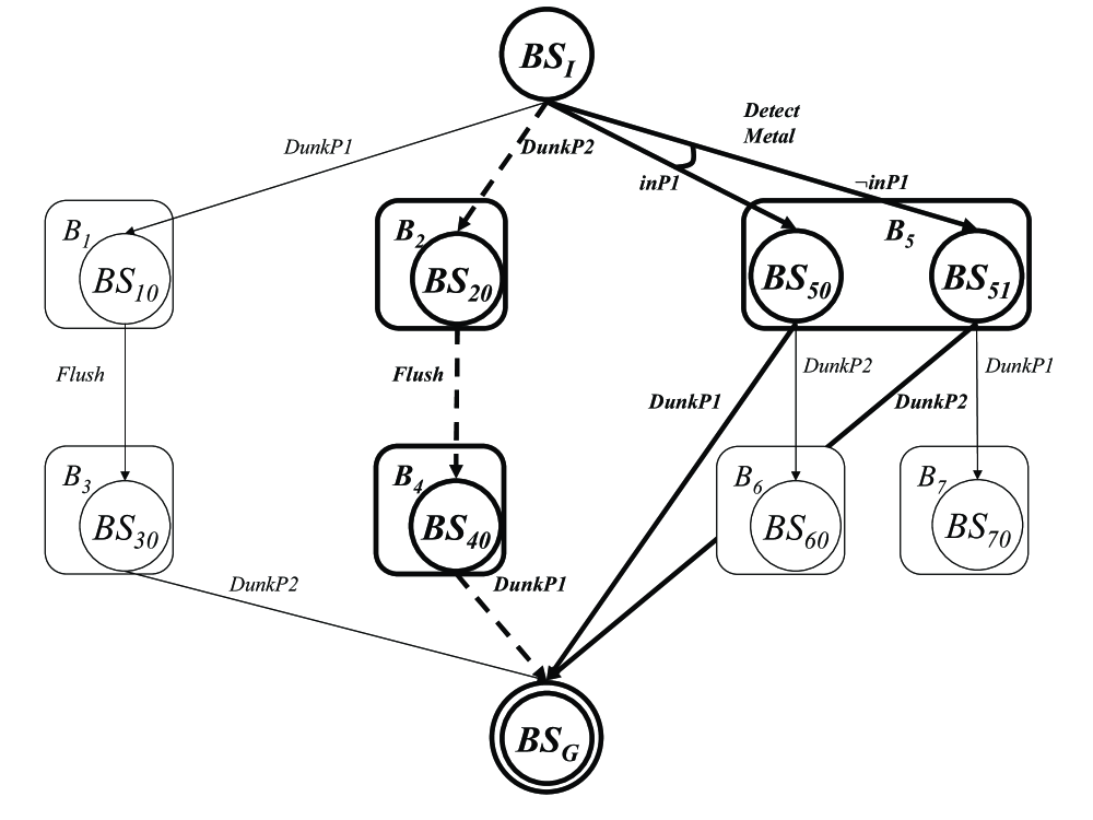
Figure 2: Illustration of progression search for a conformant plan (bold dashed edges) and a conditional plan (bold solid edges) in the BTCS problem.

We expand the leaf nodes of our best solution, a single node $BS_{10}$, with all applicable actions. The only applicable action is Flush, so we get:

$B_{3}=\{BS_{30}\}=$ Progress($BS_{10}$, Flush)
      $=$ {(inP1 $\wedge\neg$inP2 $\wedge\neg$clog $\wedge\neg$arm) $\vee$ ($\neg$inP1 $\wedge$ inP2 $\wedge\neg$clog $\wedge$ arm)}.

We assign a cost of zero to $BS_{30}$ and update our best solution. We choose Flush as the best action for $BS_{10}$ (whose cost is now one), and choose DunkP2 as the best action for $BS_{I}$ (whose cost is now one). DunkP2 is chosen for $BS_{I}$ because its successor $BS_{20}$ has a cost of zero, as opposed to $BS_{10}$ which now has a cost of one.

Expanding the leaf node $BS_{20}$ with the only applicable action, Flush, we get:

$B_{4}=\{BS_{40}\}=$ Progress($BS_{20}$, Flush)
      $=$ {($\neg$inP1 $\wedge$ inP2 $\wedge\neg$clog $\wedge$arm) $\vee$ (inP1 $\wedge\neg$inP2 $\wedge\neg$clog $\wedge\neg$ arm)}.

We update $BS_{40}$ (to have cost zero) and $BS_{20}$ (to have a cost of one), and choose Flush as the best action for $BS_{20}$. The root node $BS_{I}$ has two children, each with cost one, so we arbitrarily choose DunkP1 as the best action.

We expand $BS_{30}$ with the relevant actions to get $BS_{G}$ with the DunkP2 action. DunkP1 creates a cycle back to $BS_{10}$ so it is not added to the search graph. We now have a solution where all leaf nodes are terminal. While it is only required that a terminal belief state contains a subset of the states in $BS_{G}$, in this case the terminal belief state contains exactly the states in $BS_{G}$. The cost of the solution is three because, through revision, $BS_{30}$ has a cost of one, which sets $BS_{10}$ to a cost of two. However, this means now that $BS_{I}$ has cost of three if its best action is DunkP1. Instead, revision sets the best action for $BS_{I}$ to DunkP2 because its cost is currently two.

We then expand $BS_{40}$ with DunkP1 to find that its successor is $BS_{G}$. DunkP2 creates a cycle back to $BS_{20}$ so it is not added to the search graph. We now have our second valid solution because it contains no unexpanded leaf nodes. Revision sets the cost of $BS_{40}$ to one, $BS_{20}$ to two, and $BS_{I}$ to three. Since all solutions starting at $BS_{I}$ have equal cost (meaning there are now cheaper solutions), we can terminate with the plan DunkP2, Flush, DunkP1, shown in bold with dashed lines in Figure 2.

As an example of search for a conditional plan in $POND$, consider the BTCS example whose search graph is also shown in Figure 2. Expanding the initial belief state, we get:

$B_{1}=\{BS_{10}\}=$ Progress($BS_{I},$ DunkP1),

$B_{2}=\{BS_{20}\}=$ Progress($BS_{I},$ DunkP2),

and

$B_{5}=\{BS_{50},BS_{51}\}$ = Progress$(BS_{I},$DetectMetal)
      $=$ $\{$inP1 $\wedge\neg$inP2 $\wedge\neg$clog $\wedge$ arm, $\neg$inP1 $\wedge$ inP2 $\wedge\neg$clog $\wedge$ arm$\}$.

Each of the leaf nodes is assigned a cost of zero, and DunkP1 is chosen arbitrarily for the best solution rooted at $BS_{I}$ because the cost of each solution is identical. The cost of including each hyper-edge is the average cost of its children plus its cost, so the cost of using DetectMetal is (0+0)/2 + 1 = 1. Thus, our root $BS_{I}$ has a cost of one.

As in the conformant problem we expand $BS_{10}$, giving its child a cost of zero and $BS_{10}$ a cost of one. This changes our best solution at $BS_{I}$ to use DunkP2, and we expand $BS_{20}$, giving its child a cost of zero and it a cost of one. Then we choose DetectMetal to start the best solution at $BS_{I}$ because it gives $BS_{I}$ a cost of one, where using either Dunk action would give $BS_{I}$ a cost of two.

We expand the first child of DetectMetal, $BS_{50}$, with DunkP1 to get:

{inP1 $\wedge\neg$inP2 $\wedge$ clog $\wedge\neg$arm},

which is a goal state, and DunkP2 to get:

$B_{6}=\{BS_{60}\}$ = Progress$(BS_{50},$DunkP2) = {inP1 $\wedge\neg$inP2 $\wedge$clog $\wedge$ arm}.

We then expand the second child, $BS_{51}$, with DunkP2 to get:

{$\neg$inP1 $\wedge$ inP2 $\wedge$ clog $\wedge\neg$arm},

which is also a goal state and DunkP1 to get:

$B_{7}=\{BS_{70}\}$ = Progress$(BS_{51},$DunkP1) = {$\neg$inP1 $\wedge$ inP2 $\wedge$clog $\wedge$ arm}.

While none of these new belief states are not equivalent to $BS_{G}$, two of them entail $BS_{G}$, so we can treat them as terminal by connecting the hyper-edges for these actions to $BS_{G}$. We choose DunkP1 and DunkP2 as best actions for $BS_{50}$ and $BS_{51}$ respectively and set the cost of each node to one. This in turn sets the cost of using DetectMetal for $BS_{I}$ to (1+1)/2 + 1 = 2. We terminate here because this plan has cost equal to the other possible plans starting at $BS_{I}$ and all leaf nodes satisfy the goal. The plan is shown in bold with solid lines in Figure 2.

3 Belief State Distance

In both the CAltAlt and $POND$ planners we need to guide search node expansion with heuristics that estimate the plan distance $dist(BS,BS^{\prime})$ between two belief states $BS$ and $BS^{\prime}$. By convention, we assume $BS$ precedes $BS^{\prime}$ (i.e., in progression $BS$ is a search node and $BS^{\prime}$ is the goal belief state, or in regression $BS$ is the initial belief state and $BS^{\prime}$ is a search node). For simplicity, we limit our discussion to progression planning. Since a strong plan (executed in $BS$) ensures that every state $S\in{\cal M}(BS)$ will transition to some state $S^{\prime}\in{\cal M}(BS^{\prime})$, we define the plan distance between $BS$ and $BS^{\prime}$ as the number of actions needed to transition every state $S\in{\cal M}(BS)$ to a state $S^{\prime}\in{\cal M}(BS^{\prime})$. Naturally, in a strong plan, the actions used to transition a state $S_{1}\in{\cal M}(BS)$ may affect how we transition another state $S_{2}\in{\cal M}(BS)$. There is usually some degree of positive or negative interaction between $S_{1}$ and $S_{2}$ that can be ignored or captured in estimating plan distance. In the following we explore how to perform such estimates by using several intuitions from classical planning state distance heuristics.

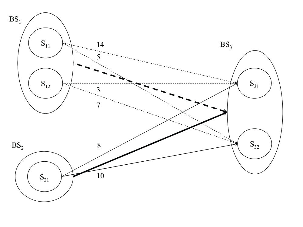
Figure 3: Conformant Plan Distance Estimation in Belief Space

We start with an example search scenario in Figure 3. There are three belief states $BS_{1}$ (containing states $S_{11}$ and $S_{12}$), $BS_{2}$ (containing state $S_{21}$), and $BS_{3}$ (containing states $S_{31}$ and $S_{32}$). The goal belief state is $BS_{3}$, and the two progression search nodes are $BS_{1}$ and $BS_{2}$. We want to expand the search node with the smallest distance to $BS_{3}$ by estimating $dist(BS_{1},BS_{3})$ – denoted by the bold, dashed line – and $dist(BS_{2},BS_{3})$ – denoted by the bold, solid line. We will assume for now that we have estimates of state distance measures $dist(S,S^{\prime})$ – denoted by the light dashed and solid lines with numbers. The state distances can be represented as numbers or action sequences. In our example, we will use the following action sequences for illustration:

$dist(S_{11},S_{32}):(\{a_{1},a_{2}\},\{a_{5}\},\{a_{6},a_{7}\})$,

$dist(S_{12},S_{31}):(\{a_{1},a_{7}\},\{a_{3}\})$,

$dist(S_{21},S_{31}):(\{a_{3},a_{6}\},\{a_{9},a_{2},a_{1}\},\{a_{0},a_{8}\},\{a_{5}\})$.

In each sequence there may be several actions in each step. For instance, $dist(S_{21},S_{31})$ has $a_{3}$ and $a_{6}$ in its first step, and there are a total of eight actions in the sequence – meaning the distance is eight. Notice that our example includes several state distance estimates, which can be found with classical planning techniques. There are many ways that we can use similar ideas to estimate belief state distance once we have addressed the issue of belief states containing several states.

Selecting States for Distance Estimation: There exists a considerable body of literature on estimating the plan distance between states in classical planning (?, ?, ?), and we would like to apply it to estimate the plan distance between two belief states, say $BS_{1}$ and $BS_{3}$. We identify four possible options for using state distance estimates to compute the distance between belief states $BS_{1}$ and $BS_{3}$:

• Sample a State Pair: We can sample a single state from $BS_{1}$ and a single state from $BS_{3}$, whose plan distance is used for the belief state distance. For example, we might sample $S_{12}$ from $BS_{1}$ and $S_{31}$ from $BS_{3}$, then define $dist(BS_{1},BS_{3})=dist(S_{12},S_{31})$.

• Aggregate States: We can form aggregate states for $BS_{1}$ and $BS_{3}$ and measure their plan distance. An aggregate state is the union of the literals needed to express a belief state formula, which we define as:

  $$\tilde{S}(BS)=\bigcup\limits_{\begin{subarray}{c}l:l\in\hat{S},\hat{S}\in\hat{\xi}(BS)\end{subarray}}l$$

  Since it is possible to express a belief state formula with every literal (e.g., using $(q\vee\neg q)\wedge p$ to express the belief state where $p$ is true), we assume a reasonably succinct representation, such as a ROBDD (?). It is quite possible the aggregate states are inconsistent, but many classical planning techniques (such as planning graphs) do not require consistent states. For example, with aggregate states we would compute the belief state distance $dist(BS_{1},BS_{3})=dist(\tilde{S}(BS_{1}),\tilde{S}(BS_{3}))$.

• Choose a Subset of States: We can choose a set of states (e.g., by random sampling) from $BS_{1}$ and a set of states from $BS_{3}$, and then compute state distances for all pairs of states from the sets. Upon computing all state distances, we can aggregate the state distances (as we will describe shortly). For example, we might sample both $S_{11}$ and $S_{12}$ from $BS_{1}$ and $S_{31}$ from $BS_{3}$, compute $dist(S_{11},S_{31})$ and $dist(S_{12},S_{31})$, and then aggregate the state distances to define $dist(BS_{1},BS_{3})$.

• Use All States: We can use all states in $BS_{1}$ and $BS_{3}$, and, similar to sampling a subset of states (above), we can compute all distances for state pairs and aggregate the distances.

The former two options for computing belief state distance are reasonably straightforward, given the existing work in classical planning. In the latter two options we compute multiple state distances. With multiple state distances there are two details which require consideration in order to obtain a belief state distance measure. In the following we treat belief states as if they contain all states because they can be appropriately replaced with the subset of chosen states.

The first issue is that some of the state distances may not be needed. Since each state in $BS_{1}$ needs to reach a state in $BS_{3}$, we should consider the distance for each state in $BS_{1}$ to “a” state in $BS_{3}$. However, we don’t necessarily need the distance for every state in $BS_{1}$ to “every” state in $BS_{3}$. We will explore assumptions about which state distances need to be computed in Section 3.1.

The second issue, which arises after computing the state distances, is that we need to aggregate the state distances into a belief state distance. We notice that the popular state distance estimates used in classical planning typically measure aggregate costs of state features (literals). Since we are planning in belief space, we wish to estimate belief state distance with the aggregate cost of belief state features (states). In Section 3.2, we will examine several choices for aggregating state distances and discuss how each captures different types of state interaction. In Section 3.3, we conclude with a summary of the choices we make in order to compute belief state distances.

3.1 State Distance Assumptions

When we choose to compute multiple state distances between two belief states $BS$ and $BS^{\prime}$, whether by considering all states or sampling subsets, not all of the state distances are important. For a given state in $BS$ we do not need to know the distance to every state in $BS^{\prime}$ because each state in $BS$ need only transition to one state in $BS^{\prime}$. There are two assumptions that we can make about the states reached in $BS^{\prime}$ which help us define two different belief state distance measures in terms of aggregate state distances:

• We can optimistically assume that each of the earlier states $S\in{\cal M}(BS)$ can reach the closest of the later states $S^{\prime}\in{\cal M}(BS^{\prime})$. With this assumption we compute distance as:

  $dist(BS,BS^{\prime})=\bigtriangledown_{S\in{\cal M}(BS)}\min\limits_{S^{\prime}\in{\cal M}(BS^{\prime})}dist(S,S^{\prime})$.

• We can assume that all of the earlier states $S\in{\cal M}(BS)$ reach the same later state $S^{\prime}\in{\cal M}(BS^{\prime})$, where the aggregate distance is minimum. With this assumption we compute distance as:

  $dist(BS,BS^{\prime})=\min\limits_{S^{\prime}\in{\cal M}(BS^{\prime})}\bigtriangledown_{S\in{\cal M}(BS)}dist(S,S^{\prime})$,

where $\bigtriangledown$ represents an aggregation technique (several of which we will discuss shortly).

Throughout the rest of the paper we use the first definition for belief state distance because it is relatively robust and easy to compute. Its only drawback is that it treats the earlier states in a more independent fashion, but is flexible in allowing earlier states to transition to different later states. The second definition measures more dependencies of the earlier states, but restricts them to reach the same later state. While the second may sometimes be more accurate, it is misinformed in cases where all earlier states cannot reach the same later state (i.e., the measure would be infinite). We do not pursue the second method because it may return distance measures that are infinite when they are in fact finite.

As we will see in Section 4, when we discuss computing these measures with planning graphs, we can implicitly find for each state in $BS$ the closest state in $BS^{\prime}$, so that we do not enumerate the states $S^{\prime}$ in the minimization term of the first belief state distance (above). Part of the reason we can do this is that we compute distance in terms of constituents $\hat{S}^{\prime}\in\hat{\xi}(BS^{\prime})$ rather than actual states. Also, because we only consider constituents of $BS^{\prime}$, when we discuss sampling belief states to include in distance computation we only sample from $BS$. We can also avoid the explicit aggregation $\bigtriangledown$ by using the $LUG$, but describe several choices for $\bigtriangledown$ to understand implicit assumptions made by the heuristics computed on the $LUG$.

3.2 State Distance Aggregation

The aggregation function $\bigtriangledown$ plays an important role in how we measure the distance between belief states. When we compute more than one state distance measure, either exhaustively or by sampling a subset (as previously mentioned), we must combine the measures by some means, denoted $\bigtriangledown$. There is a range of options for taking the state distances and aggregating them into a belief state distance. We discuss several assumptions associated with potential measures:

• Positive Interaction of States: Positive interaction assumes that the most difficult state in $BS$ requires actions that will help transition all other states in $BS$ to some state in $BS^{\prime}$. In our example, this means that we assume the actions used to transition $S_{11}$ to $S_{32}$ will help us transition $S_{12}$ to $S_{31}$ (assuming each state in $BS_{1}$ transitions to the closest state in $BS_{3}$). Inspecting the action sequences, we see they positively interact because both need actions $a_{1}$ and $a_{7}$. We do not need to know the action sequences to assume positive interaction because we define the aggregation $\bigtriangledown$ as a maximization of numerical state distances:

  $dist(BS,BS^{\prime})=\max\limits_{S\in{\cal M}(BS)}\min\limits_{S^{\prime}\in{\cal M}(BS^{\prime})}dist(S,S^{\prime})$.

  The belief state distances are $dist(BS_{1},BS_{3})=\max(\min(14,5),$ $\min(3,7))=5$ and $dist(BS_{2},BS_{3})=\max(\min(8,10))=8$. In this case we prefer $BS_{1}$ to $BS_{2}$. If each state distance is admissible and we do not sample from belief states, then assuming positive interaction is also admissible.

• Independence of States: Independence assumes that each state in $BS$ requires actions that are different from all other states in $BS$ in order to reach a state in $BS^{\prime}$. Previously, we found there was positive interaction in the action sequences to transition $S_{11}$ to $S_{32}$ and $S_{12}$ to $S_{31}$ because they shared actions $a_{1}$ and $a_{7}$. There is also some independence in these sequences because the first contains $a_{2},a_{5}$, and $a_{6}$, where the second contains $a_{3}$. Again, we do not need to know the action sequences to assume independence because we define the aggregation $\bigtriangledown$ as a summation of numerical state distances:

  $dist(BS,BS^{\prime})=\sum\limits_{S\in{\cal M}(BS)}\min\limits_{S^{\prime}\in{\cal M}(BS^{\prime})}dist(S,S^{\prime})$.

  In our example, $dist(BS_{1},BS_{3})=\min(14,5)+\min(3,7)=8$, and $dist(BS_{2},BS_{3})=\min(8,10)=8$. In this case we have no preference over $BS_{1}$ and $BS_{2}$.

  We notice that using the cardinality of a belief state $|{\cal M}(BS)|$ to measure $dist(BS,BS^{\prime})$ is a special case of assuming state independence, where $\forall S,S^{\prime}dist(S,S^{\prime})=1$. If we use cardinality to measure distance in our example, then we have $dist(BS_{1},BS_{3})=|{\cal M}(BS_{1})|=2$, and $dist(BS_{2},BS_{3})=|{\cal M}(BS_{2})|=1$. With cardinality we prefer $BS_{2}$ over $BS_{1}$ because we have better knowledge in $BS_{2}$.

• Overlap of States: Overlap assumes that there is both positive interaction and independence between the actions used by states in $BS$ to reach a state in $BS^{\prime}$. The intuition is that some actions can often be used for multiple states in $BS$ simultaneously and we should count these actions only once. For example, when we computed $dist(BS_{1},BS_{3})$ by assuming positive interaction, we noticed that the action sequences for $dist(S_{11},S_{32})$ and $dist(S_{12},S_{31})$ both used $a_{1}$ and $a_{7}$. When we aggregate these sequences we would like to count $a_{1}$ and $a_{7}$ each only once because they potentially overlap. However, truly combining the action sequences for maximal overlap is a plan merging problem (?), which can be as difficult as planning. Since our ultimate intent is to compute heuristics, we take a very simple approach to merging action sequences. We introduce a plan merging operator $\Cup$ for $\bigtriangledown$ that picks a step at which we align the sequences and then unions the aligned steps. We use the size of the resulting action sequence to measure belief state distance:

  $dist(BS,BS^{\prime})=\Cup_{S\in{\cal M}(BS)}\min\limits_{S^{\prime}\in{\cal M}(BS^{\prime})}dist(S,S^{\prime})$.

  Depending on the type of search, we define $\Cup$ differently. We assume that sequences used in progression search start at the same time and those used in regression end at the same time. Thus, in progression all sequences are aligned at the first step before we union steps, and in regression all sequences are aligned at the last step before the union.

  For example, in progression $dist(S_{11},S_{32})\Cup dist(S_{12},S_{31})$ $=(\{a_{1},a_{2}\},\{a_{5}\},\{a_{6},a_{7}\})\Cup(\{a_{1},a_{7}\},\{a_{3}\})$ $=(\{a_{1},a_{2},a_{7}\},\{a_{5},a_{3}\},\{a_{6},$ $a_{7}\})$ because we align the sequences at their first steps, then union each step. Notice that this resulting sequence has seven actions, giving $dist(BS_{1},BS_{3})=7$, whereas defining $\bigtriangledown$ as maximum gave a distance of five and as summation gave a distance of eight. Compared with overlap, positive interaction tends to under estimate distance, and independence tends to over estimate distance. As we will see during our empirical evaluation (in Section 6.5), accounting for overlap provides more accurate distance measures for many conformant planning domains.

• Negative Interaction of States: Negative interaction between states can appear in our example if transitioning state $S_{11}$ to state $S_{32}$ makes it more difficult (or even impossible) to transition state $S_{12}$ to state $S_{31}$. This could happen if performing action $a_{5}$ for $S_{11}$ conflicts with action $a_{3}$ for $S_{12}$. We can say that $BS_{1}$ cannot reach $BS_{3}$ if all possible action sequences that start in $S_{11}$ and $S_{12}$, respectively, and end in any $S\in{\cal M}(BS_{3})$ negatively interact.

  There are two ways negative interactions play a role in belief state distances. Negative interactions can allow us to prove it is impossible for a belief state $BS$ to reach a belief state $BS^{\prime}$, meaning $dist(BS,BS^{\prime})=\infty$, or they can potentially increase the distance by a finite amount. We use only the first, more extreme, notion of negative interaction by computing “cross-world” mutexes (?) to prune belief states from the search. If we cannot prune a belief state, then we use one of the aforementioned techniques to aggregate state distances. As such, we do not provide a concrete definition for $\bigtriangledown$ to measure negative interaction.

  While we do not explore ways to adjust the distance measure for negative interactions, we mention some possibilities. Like work in classical planning (?), we can penalize the distance measure $dist(BS_{1},BS_{3})$ to reflect additional cost associated with serializing conflicting actions. Additionally in conditional planning, conflicting actions can be conditioned on observations so that they do not execute in the same plan branch. A distance measure that uses observations would reflect the added cost of obtaining observations, as well as the change in cost associated with introducing plan branches (e.g., measuring average branch cost).

The above techniques for belief state distance estimation in terms of state distances provide the basis for our use of multiple planning graphs. We will show in the empirical evaluation that these measures affect planner performance very differently across standard conformant and conditional planning domains. While it can be quite costly to compute several state distance measures, understanding how to aggregate state distances sets the foundation for techniques we develop in the $LUG$. As we have already mentioned, the $LUG$ conveniently allows us to implicitly aggregate state distances to directly measure belief state distance.

3.3 Summary of Methods for Distance Estimation

Since we explore several methods for computing belief state distances on planning graphs, we provide a summary of the choices we must consider, listed in Table 1. Each column is headed with a choice, containing possible options below. The order of the columns reflects the order in which we consider the options.

State	State Distance	Planning	Mutex	Mutex	Heuristic
Selection	Aggregation	Graph	Type	Worlds
Single	+ Interaction	$SG$	None	Same	Max
Aggregate	Independence	$MG$	Static	Intersect	Sum
Subset	Overlap	$LUG$	Dynamic	Cross	Level
All	- Interaction		Induced		Relaxed Plan

Table 1: Features for a belief state distance estimation.

In this section we have covered the first two columns which relate to selecting states from belief states for distance computation, as well as aggregating multiple state distances into a belief state distance. We test options for both of these choices in the empirical evaluation.

In the next section we will also expand upon how to aggregate distance measures as well as discuss the remaining columns of Table 1. We will present each type of planning graph: the single planning graph ($SG$), multiple planning graphs ($MG$), and the labelled uncertainty graph ($LUG$). Within each planning graph we will describe several types of mutex, including static, dynamic, and induced mutexes. Additionally, each type of mutex can be computed with respect to different possible worlds – which means the mutex involves planning graph elements (e.g., actions) when they exist in the same world (i.e., mutexes are only computed within the planning graph for a single state), or across worlds (i.e., mutexes are computed between planning graphs for different states) by two methods (denoted Intersect and Cross). Finally, we can compute many different heuristics on the planning graphs to measure state distances – max, sum, level, and relaxed plan. We focus our discussion on the planning graphs, same-world mutexes, and relaxed plan heuristics in the next section. Cross-world mutexes and the other heuristics are described in appendices.

4 Heuristics

This section discusses how we can use planning graph heuristics to measure belief state distances. We cover several types of planning graphs and the extent to which they can be used to compute various heuristics. We begin with a brief background on planning graphs.

Planning Graphs: Planning graphs serve as the basis for our belief state distance estimation. Planning graphs were initially introduced in GraphPlan (?) for representing an optimistic, compressed version of the state space progression tree. The compression lies in unioning the literals from every state at subsequent steps from the initial state. The optimism relates to underestimating the number of steps it takes to support sets of literals (by tracking only a subset of the infeasible tuples of literals). GraphPlan searches the compressed progression (or planning graph) once it achieves the goal literals in a level with no two goal literals marked infeasible. The search tries to find actions to support the top level goal literals, then find actions to support the chosen actions and so on until reaching the first graph level. The basic idea behind using planning graphs for search heuristics is that we can find the first level of a planning graph where a literal in a state appears; the index of this level is a lower bound on the number of actions that are needed to achieve a state with the literal. There are also techniques for estimating the number of actions required to achieve sets of literals. The planning graphs serve as a way to estimate the reachability of state literals and discriminate between the “goodness” of different search states. This work generalizes such literal estimations to belief space search by considering both GraphPlan and CGP style planning graphs plus a new generalization of planning graphs, called the $LUG$.

Planners such as CGP (?) and SGP (?) adapt the GraphPlan idea of compressing the search space with a planning graph by using multiple planning graphs, one for each possible world in the initial belief state. CGP and SGP search on these planning graphs, similar to GraphPlan, to find conformant and conditional plans. The work in this paper seeks to apply the idea of extracting search heuristics from planning graphs, previously used in state space search (?, ?, ?) to belief space search.

Planning Graphs for Belief Space: This section proceeds by describing four classes of heuristics to estimate belief state distance $NG,SG,MG,$ and $LUG$. $NG$ heuristics are techniques existing in the literature that are not based on planning graphs, $SG$ heuristics are techniques based on a single classical planning graph, $MG$ heuristics are techniques based on multiple planning graphs (similar to those used in CGP) and $LUG$ heuristics use a new labelled planning graph. The $LUG$ combines the advantages of $SG$ and $MG$ to reduce the representation size and maintain informedness. Note that we do not include observations in any of the planning graph structures as SGP (?) would, however we do include this feature for future work. The conditional planning formulation directly uses the planning graph heuristics by ignoring observations, and our results show that this still gives good performance.

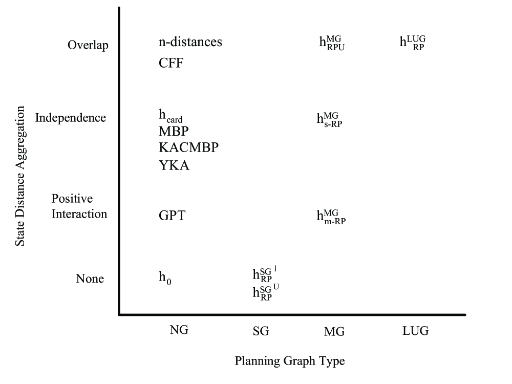
Figure 4: Taxonomy of heuristics with respect to planning graph type and state distance aggregation. Blank entries indicate that the combination is meaningless or not possible.

In Figure 4 we present a taxonomy of distance measures for belief space. The taxonomy also includes related planners, whose distance measures will be characterized in this section. All of the related planners are listed in the $NG$ group, despite the fact that some actually use planning graphs, because they do not clearly fall into one of our planning graph categories. The figure shows how different substrates (horizontal axis) can be used to compute belief state distance by aggregating state to state distances under various assumptions (vertical axis). Some of the combinations are not considered because they do not make sense or are impossible. The reasons for these omissions will be discussed in subsequent sections. While there are a wealth of different heuristics one can compute using planning graphs, we concentrate on relaxed plans because they have proven to be the most effective in classical planning and in our previous studies (?). We provide additional descriptions of other heuristics like max, sum, and level in Appendix A.

Example: To illustrate the computation of each heuristic, we use an example derived from BTC called Courteous BTC (CBTC) where a courteous package dunker has to disarm the bomb and leave the toilet unclogged, but some discourteous person has left the toilet clogged. The initial belief state of CBTC in clausal representation is:

$\kappa(BS_{I})=$ arm $\wedge$ clog $\wedge$ (inP1 $\vee$ inP2) $\wedge$ ($\neg$inP1 $\vee\neg$inP2),

and the goal is:

$\kappa(BS_{G})=$ $\neg$clog $\wedge\neg$arm.

The optimal action sequences to reach $BS_{G}$ from $BS_{I}$ are:

Flush, DunkP1, Flush, DunkP2, Flush,

and

Flush, DunkP2, Flush, DunkP1, Flush.

Thus the optimal heuristic estimate for the distance between $BS_{I}$ and $BS_{G}$, in regression, is $h^{*}(BS_{G})$ = 5 because in either plan there are five actions.

We use planning graphs for both progression and regression search. In regression search the heuristic estimates the cost of the current belief state w.r.t. the initial belief state and in progression search the heuristic estimates the cost of the goal belief state w.r.t. the current belief state. Thus, in regression search the planning graph(s) are built (projected) once from the possible worlds of the initial belief state, but in progression search they need to be built at each search node. We introduce a notation $BS_{i}$ to denote the belief state for which we find a heuristic measure, and $BS_{P}$ to denote the belief state that is used to construct the initial layer of the planning graph(s). In the following subsections we describe computing heuristics for regression, but they are generalized for progression by changing $BS_{i}$ and $BS_{P}$ appropriately.

In the previous section we discussed two important issues involved in heuristic computation: sampling states to include in the computation and using mutexes to capture negative interactions in the heuristics. We will not directly address these issues in this section, deferring them to discussion in the respective empirical evaluation sections, 6.4 and 6.2. The heuristics below are computed once we have decided on a set of states to use, whether by sampling or not. Also, as previously mentioned, we only consider sampling states from the belief state $BS_{P}$ because we can implicitly find closest states from $BS_{i}$ without sampling. We only explore computing mutexes on the planning graphs in regression search. We use mutexes to determine the first level of the planning graph where the goal belief state is reachable (via the level heuristic described in Appendix A) and then extract a relaxed plan starting at that level. If the level heuristic is $\infty$ because there is no level where a belief state is reachable, then we can prune the regressed belief state.

We proceed by describing the various substrates used for computing belief space distance estimates. Within each we describe the prospects for various types of world aggregation. In addition to our heuristics, we mention related work in the relevant areas.

4.1 Non Planning Graph-based Heuristics ($NG$)

We group many heuristics and planners into the $NG$ group because they are not using $SG$, $MG$, or $LUG$ planning graphs. Just because we mention them in this group does not mean they are not using planning graphs in some other form.

No Aggregation: Breadth first search uses a simple heuristic, $h_{0}$ where the heuristic value is set to zero. We mention this heuristic so that we can gauge the effectiveness of our search substrates relative to improvements gained through using heuristics.

Positive Interaction Aggregation: The GPT planner (?) measures belief state distance as the maximum of the minimum state to state distance of states in the source and destination belief states, assuming optimistic reachability as mentioned in Section 3. GPT measures state distances exactly, in terms of the minimum number of transitions in the state space. Taking the maximum state to state distance is akin to assuming positive interaction of states in the current belief state.

Independence Aggregation: The MBP planner (?), KACMBP planner (?), YKA planner (?), and our comparable $h_{card}$ heuristic measure belief state distance by assuming every state to state distance is one, and taking the summation of the state distances (i.e. counting the number of states in a belief state). This measure can be useful in regression because goal belief states are partially specified and contain many states consistent with a goal formula and many of the states consistent with the goal formula are not reachable from the initial belief state. Throughout regression, many of the unreachable states are removed from predecessor belief states because they are inconsistent with the preconditions of a regressed action. Thus, belief states can reduce in size during regression and their cardinality may indicate they are closer to the initial belief state. Cardinality is also useful in progression because as belief states become smaller, the agent has more knowledge and it can be easier to reach a goal state.

In CBTC, $h_{card}(BS_{G})=4$ because $BS_{G}$ has four states consistent with its complete representation:

$\xi(BS_{G})=$ ($\neg$inP1 $\wedge\neg$inP2$\wedge\neg$clog $\wedge\neg$arm) $\vee$ ($\neg$inP1 $\wedge$ inP2 $\wedge\neg$clog $\wedge\neg$arm) $\vee$
                 (inP1 $\wedge\neg$inP2 $\wedge\neg$clog $\wedge\neg$arm) $\vee$ (inP1 $\wedge$ inP2 $\wedge\neg$clog $\wedge\neg$arm).

Notice, this may be uninformed for $BS_{G}$ because two of the states in $\xi(BS_{G})$ are not reachable, like: (inP1 $\wedge$ inP2 $\wedge\neg$clog $\wedge\neg$arm). If there are $n$ packages, then there would be $2^{n-1}$ unreachable states represented by $\xi(BS_{G})$. Counting unreachable states may overestimate the distance estimate because we do not need to plan for them. In general, in addition to the problem of counting unreachable states, cardinality does not accurately reflect distance measures. For instance, MBP reverts to breadth first search in classical planning problems because state distance may be large or small but it still assigns a value of one.

Overlap Aggregation: ? (?) describes n-Distances which generalize the belief state distance measure in GPT to consider the maximum n-tuple state distance. The measure involves, for each n-sized tuple of states in a belief state, finding the length of the actual plan to transition the n-tuple to the destination belief state. Then the maximum n-tuple distance is taken as the distance measure.

For example, consider a belief state with four states. With an n equal to two, we would define six belief states, one for each size two subset of the four states. For each of these belief states we find a real plan, then take the maximum cost over these plans to measure the distance for the original four state belief state. When n is one, we are computing the same measure as GPT, and when n is equal to the size of the belief state we are directly solving the planning problem. While it is costly to compute this measure for large values of n, it is very informed as it accounts for overlap and negative interactions.

The CFF planner (?) uses a version of a relaxed planning graph to extract relaxed plans. The relaxed plans measure the cost of supporting a set of goal literals from all states in a belief state. In addition to the traditional notion of a relaxed planning graph that ignores mutexes, CFF also ignores all but one antecedent literal in conditional effects to keep their relaxed plan reasoning tractable. The CFF relaxed plan does capture overlap but ignores some subgoals and all mutexes. The way CFF ensures the goal is supported in the relaxed problem is to encode the relaxed planning graph as a satisfiability problem. If the encoding is satisfiable, the chosen number of action assignments is the distance measure.

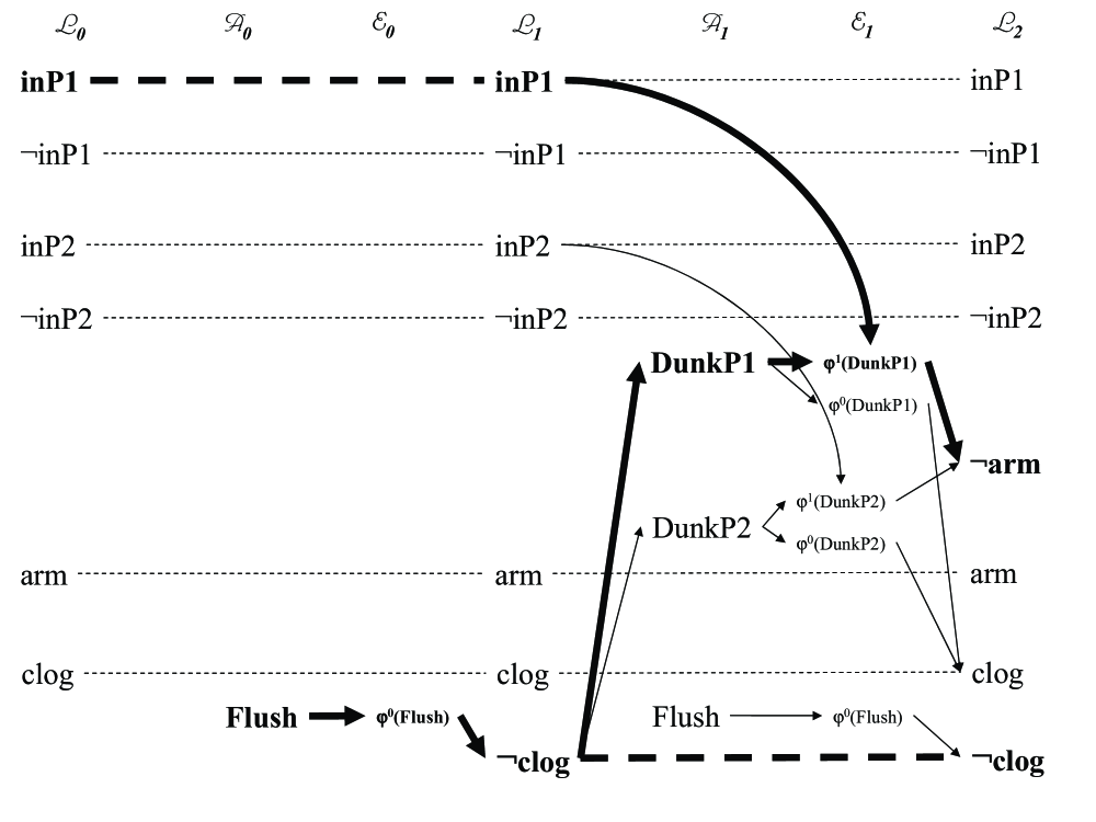
Figure 5: Single planning graph for CBTC, with relaxed plan components in bold. Mutexes omitted.

4.2 Single Graph Heuristics ($SG$)

The simplest approach for using planning graphs for belief space planning heuristics is to use a “classical” planning graph. To form the initial literal layer from the projected belief state, we could either sample a single state (denoted $SG^{1}$) or use an aggregate state (denoted $SG^{U}$). For example, in CBTC (see Figure 5) assuming regression search with $BS_{P}=BS_{I}$, the initial level ${\cal L}_{0}$ of the planning graph for $SG^{1}$ might be:

${\cal L}_{0}$ = {arm, clog, inP1, $\neg$inP2}

and for $SG^{U}$ it is defined by the aggregate state $\tilde{S}(BS_{P})$:

${\cal L}_{0}$ = {arm, clog, inP1, inP2, $\neg$inP1, $\neg$inP2}.

Since these two versions of the single planning graph have identical semantics, aside from the initial literal layer, we proceed by describing the $SG^{U}$ graph and point out differences with $SG^{1}$ where they arise.

Graph construction is identical to classical planning graphs (including mutex propagation) and stops when two subsequent literal layers are identical (level off). We use the planning graph formalism used in IPP (?) to allow for explicit representation of conditional effects, meaning there is a literal layer ${\cal L}_{k}$, an action layer ${\cal A}_{k}$, and an effect layer ${\cal E}_{k}$ in each level $k$. Persistence for a literal $l$, denoted by $l_{p}$, is represented as an action where $\rho^{e}(l_{p})=\varepsilon^{0}(l_{p})=l$. A literal is in ${\cal L}_{k}$ if an effect from the previous effect layer ${\cal E}_{k-1}$ contains the literal in its consequent. An action is in the action layer ${\cal A}_{k}$ if every one of its execution precondition literals is in ${\cal L}_{k}$. An effect is in the effect layer ${\cal E}_{k}$ if its associated action is in the action layer ${\cal A}_{k}$ and every one of its antecedent literals is in ${\cal L}_{k}$. Using conditional effects in the planning graph avoids factoring an action with conditional effects into a possibly exponential number of non-conditional actions, but adds an extra planning graph layer per level. Once our graph is built, we can extract heuristics.

No Aggregation: Relaxed plans within a single planning graph are able to measure, under the most optimistic assumptions, the distance between two belief states. The relaxed plan represents a distance between a subset of the initial layer literals and the literals in a constituent of our belief state. In the $SG^{U}$, the literals from the initial layer that are used for support may not hold in a single state of the projected belief state, unlike the $SG^{1}$. The classical relaxed plan heuristic $h^{SG}_{RP}$ finds a set of (possibly interfering) actions to support the goal constituent. The relaxed plan $RP$ is a subgraph of the planning graph, of the form {${\cal A}^{RP}_{0}$, ${\cal E}^{RP}_{0}$, ${\cal L}^{RP}_{1}$, …, ${\cal A}^{RP}_{b-1}$, ${\cal E}^{RP}_{b-1}$, ${\cal L}^{RP}_{b}$}. Each of the layers contains a subset of the vertices in the corresponding layer of the planning graph.

More formally, we find the relaxed plan to support the constituent $\hat{S}\in\hat{\xi}(BS_{i})$ that is reached earliest in the graph (as found by the $h^{SG}_{level}(BS_{i})$ heuristic in Appendix A). Briefly, $h^{SG}_{level}(BS_{i})$ returns the first level $b$ where a constituent of $BS_{i}$ has all its literals in ${\cal L}_{b}$ and none are marked pair-wise mutex. Notice that this is how we incorporate negative interactions into our heuristics. We start extraction at the level $b$, by defining ${\cal L}^{RP}_{b}$ as the literals in the constituent used in the level heuristic. For each literal $l\in{\cal L}^{RP}_{b}$, we select a supporting effect (ignoring mutexes) from ${\cal E}_{b-1}$ to form the subset ${\cal E}^{RP}_{b-1}$. We prefer persistence of literals to effects in supporting literals. Once a supporting set of effects is found, we create ${\cal A}^{RP}_{b-1}$ as all actions with an effect in ${\cal E}^{RP}_{b-1}$. Then the needed preconditions for the actions and antecedents for chosen effects in ${\cal A}^{RP}_{b-1}$ and ${\cal E}^{RP}_{b-1}$ are added to the list of literals to support from ${\cal L}^{RP}_{b-2}$. The algorithm repeats until we find the needed actions from ${\cal A}_{0}$. A relaxed plan’s value is the summation of the number of actions in each action layer. A literal persistence, denoted by a subscript “p”, is treated as an action in the planning graph, but in a relaxed plan we do not include it in the final computation of $\mid{{\cal A}^{RP}_{j}}\mid$. The single graph relaxed plan heuristic is computed as

$$h^{SG}_{RP}(BS_{i})=\sum\limits_{j=0}^{b-1}\mid{{\cal A}^{RP}_{j}}\mid$$

For the CBTC problem we find a relaxed plan from the $SG^{U}$, as shown in Figure 5 as the bold edges and nodes. Since $\neg$arm and $\neg$clog are non mutex at level two, we can use persistence to support $\neg$clog and DunkP1 to support $\neg$arm in ${\cal L}^{RP}_{2}$. In ${\cal L}^{RP}_{1}$ we can use persistence for inP1, and Flush for $\neg$clog. Thus, $h^{SG}_{RP}(BS_{G})$ = 2 because the relaxed plan is:

${\cal A}^{RP}_{0}=\{$inP1_p, Flush$\}$,

${\cal E}^{RP}_{0}=\{\varphi^{0}($inP1${}_{p})$, $\varphi^{0}($Flush$)$},

${\cal L}^{RP}_{1}=\{$inP1$,\neg$clog$\}$,

${\cal A}^{RP}_{1}=\{\neg$clog_p, DunkP1$\}$,

${\cal E}^{RP}_{1}=\{\varphi^{0}(\neg$clog${}_{p})$, $\varphi^{1}($DunkP1$)$},

${\cal L}^{RP}_{2}=\{\neg$arm$,\neg$clog$\}$.

The relaxed plan does not use both DunkP2 and DunkP1 to support $\neg$arm. As a result $\neg$arm is not supported in all worlds (i.e. it is not supported when the state where inP2 holds is our initial state). Our initial literal layer threw away knowledge of inP1 and inP2 holding in different worlds, and the relaxed plan extraction ignored the fact that $\neg$arm needs to be supported in all worlds. Even with an $SG^{1}$ graph, we see similar behavior because we are reasoning with only a single world. A single, unmodified classical planning graph cannot capture support from all possible worlds – hence there is no explicit aggregation over distance measures for states. As a result, we do not mention aggregating states to measure positive interaction, independence, or overlap.

4.3 Multiple Graph Heuristics ($MG$)

Single graph heuristics are usually uninformed because the projected belief state $BS_{P}$ often corresponds to multiple possible states. The lack of accuracy is because single graphs are not able to capture propagation of multiple world support information. Consider the CBTC problem where the projected belief state is $BS_{I}$ and we are using a single graph $SG^{U}$. If DunkP1 were the only action we would say that $\neg$arm and $\neg$clog can be reached at a cost of two, but in fact the cost is infinite (since there is no DunkP2 to support $\neg$arm from all possible worlds), and there is no strong plan.

To account for lack of support in all possible worlds and sharpen the heuristic estimate, a set of multiple planning graphs $\Gamma$ is considered. Each $\gamma\in\Gamma$ is a single graph, as previously discussed. These multiple graphs are similar to the graphs used by CGP (?), but lack the more general cross-world mutexes. Mutexes are only computed within each graph, i.e. only same-world mutexes are computed. We construct the initial layer ${\cal L}^{\gamma}_{0}$ of each graph $\gamma$ with a different state $S\in{\cal M}(BS_{P})$. With multiple graphs, the heuristic value of a belief state is computed in terms of all the graphs. Unlike single graphs, we can compute different world aggregation measures with the multiple planning graphs.

While we get a more informed heuristic by considering more of the states in ${\cal M}(BS_{P})$, in certain cases it can be costly to compute the full set of planning graphs and extract relaxed plans. We will describe computing the full set of planning graphs, but will later evaluate (in Section 6.4) the effect of computing a smaller proportion of these. The single graph $SG^{1}$ is the extreme case of computing fewer graphs.

To illustrate the use of multiple planning graphs, consider our example CBTC. We build two graphs (Figure 6) for the projected $BS_{P}$. They have the respective initial literal layers:

${\cal L}^{1}_{0}=\{$arm, clog, inP1, $\neg$inP2$\}$ and

${\cal L}^{2}_{0}=\{$arm, clog, $\neg$inP2, inP2$\}$.

In the graph for the first possible world, $\neg$arm comes in only through DunkP1 at level 2. In the graph for the second world, $\neg$arm comes in only through DunkP2 at level 2. Thus, the multiple graphs show which actions in the different worlds contribute to support the same literal.

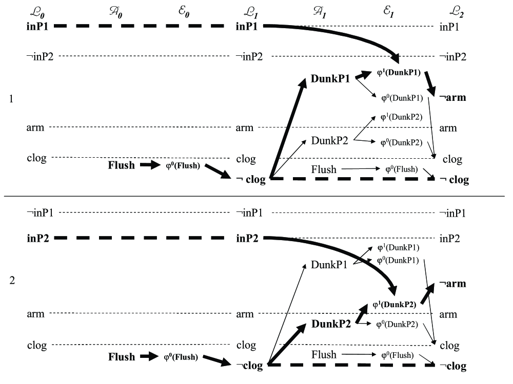
Figure 6: Multiple planning graphs for CBTC, with relaxed plan components bolded. Mutexes omitted.

A single planning graph is sufficient if we do not aggregate state measures, so in the following we consider how to compute the achievement cost of a belief state with multiple graphs by aggregating state distances.

Positive Interaction Aggregation: Similar to GPT (?), we can use the worst-case world to represent the cost of the belief state $BS_{i}$ by using the $h^{MG}_{m-RP}$ heuristic. The difference with GPT is that we compute a heuristic on planning graphs, where they compute plans in state space. With this heuristic we account for the number of actions used in a given world, but assume positive interaction across all possible worlds.

The $h^{MG}_{m-RP}$ heuristic is computed by finding a relaxed plan $RP_{\gamma}$ on each planning graph $\gamma\in\Gamma$, exactly as done on the single graph with $h^{SG}_{RP}$. The difference is that unlike the single graph relaxed plan $SG^{U}$, but like $SG^{1}$, the initial levels of the planning graphs are states, so each relaxed plan will reflect all the support needed in the world corresponding to $\gamma$. Formally:

$$h^{MG}_{m-RP}(BS_{i})=\max\limits_{\gamma\in{\Gamma}}\left(\sum\limits_{j=0}^{b_{\gamma}-1}\mid{{\cal A}^{RP_{\gamma}}_{j}}\mid\right)$$

where $b_{\gamma}$ is the level of $\gamma$ where a constituent of $BS_{G}$ was first reachable.

Notice that we are not computing all state distances between states in $BS_{P}$ and $BS_{i}$. Each planning graph $\gamma$ corresponds to a state in $BS_{P}$, and from each $\gamma$ we extract a single relaxed plan. We do not need to enumerate all states in $BS_{i}$ and find a relaxed plan for each. We instead support a set of literals from one constituent of $BS_{i}$. This constituent is estimated to be the minimum distance state in $BS_{i}$ because it is the first constituent reached in $\gamma$.

For CBTC, computing $h^{MG}_{m-RP}(BS_{G})$ (Figure 6) finds:

${RP}_{1}=$

${\cal A}^{RP_{1}}_{0}=\{$inP1_p, Flush$\}$,

${\cal E}^{RP_{1}}_{0}=\{\varphi^{0}($inP1${}_{p})$, $\varphi^{0}($Flush$)$},

${\cal L}^{RP_{1}}_{1}=\{$inP1$,\neg$clog$\}$,

${\cal A}^{RP_{1}}_{1}=\{\neg$clog_p, DunkP1$\}$,

${\cal E}^{RP_{1}}_{1}=\{\varphi^{0}(\neg$clog${}_{p})$, $\varphi^{1}($DunkP1$)$},

${\cal L}^{RP_{1}}_{2}=\{\neg$arm$,\neg$clog$\}$

and ${RP}_{2}=$

${\cal A}^{RP_{2}}_{0}=\{$inP2_p, Flush$\}$,

${\cal E}^{RP_{2}}_{0}=\{\varphi^{0}($inP2${}_{p})$, $\varphi^{0}($Flush$)$},

${\cal L}^{RP_{2}}_{1}=\{$inP2$,\neg$clog$\}$,

${\cal A}^{RP_{2}}_{1}=\{\neg$clog_p, DunkP2$\}$,

${\cal E}^{RP_{2}}_{1}=\{\varphi^{0}(\neg$clog${}_{p})$, $\varphi^{1}($DunkP2$)$},

${\cal L}^{RP_{2}}_{2}=\{\neg$arm$,\neg$clog$\}$.

Each relaxed plan contains two actions and taking the maximum of the two relaxed plan values gives $h^{MG}_{m-RP}(BS_{G})=2$. This aggregation ignores the fact that we must use different Dunk actions each possible world.

Independence Aggregation: We can use the $h^{MG}_{s-RP}$ heuristic to assume independence among the worlds in our belief state. We extract relaxed plans exactly as described in the previous heuristic and simply use a summation rather than maximization of the relaxed plan costs. Formally:

$$h^{MG}_{s-RP}(BS_{i})=\sum\limits_{\gamma\in{\Gamma}}\left(\sum\limits_{j=0}^{b_{\gamma}-1}\mid{{\cal A}^{RP_{\gamma}}_{j}}\mid\right)$$

where $b_{\gamma}$ is the level of $\gamma$ where a constituent of $BS_{G}$ was first reachable.

For CBTC, if computing $h^{MG}_{s-RP}(BS_{G})$, we find the same relaxed plans as in the $h^{MG}_{m-RP}(BS_{G})$ heuristic, but sum their values to get 2 + 2 = 4 as our heuristic. This aggregation ignores the fact that we can use the same Flush action for both possible worlds.

State Overlap Aggregation: We notice that in the two previous heuristics we are either taking a maximization and not accounting for some actions, or taking a summation and possibly accounting for extra actions. We present the $h^{MG}_{RPU}$ heuristic to balance the measure between positive interaction and independence of worlds. Examining the relaxed plans computed by the two previous heuristics for the CBTC example, we see that the relaxed plans extracted from each graph have some overlap. Notice, that both ${\cal A}^{RP_{1}}_{0}$ and ${\cal A}^{RP_{2}}_{0}$ contain a Flush action irrespective of which package the bomb is in – showing some positive interaction. Also, ${\cal A}^{RP_{1}}_{1}$ contains DunkP1, and ${\cal A}^{RP_{2}}_{1}$ contains DunkP2 – showing some independence. If we take the layer-wise union of the two relaxed plans, we would get a unioned relaxed plan:

$RP_{U}=$

${\cal A}^{RP_{U}}_{0}=\{$inP1_p, Flush$\}$,

${\cal E}^{RP_{U}}_{0}=\{\varphi^{0}($inP1${}_{p})$, $\varphi^{0}($inP2${}_{p})$, $\varphi^{0}($Flush$)$},

${\cal L}^{RP_{U}}_{1}=\{$inP1, inP2$,\neg$clog$\}$,

${\cal A}^{RP_{U}}_{1}=\{\neg$clog_p, DunkP1, DunkP2$\}$,

${\cal E}^{RP_{U}}_{1}=\{\varphi^{0}(\neg$clog${}_{p})$, $\varphi^{1}($DunkP1$)$, $\varphi^{1}($DunkP2$)$},

${\cal L}^{RP_{U}}_{2}=\{\neg$arm$,\neg$clog$\}$.

This relaxed plans accounts for the actions that are the same between possible worlds and the actions that differ. Notice that Flush appears only once in layer zero and the Dunk actions both appear in layer one.

In order to get the union of relaxed plans, we extract relaxed plans from each $\gamma\in{\Gamma}$, as in the two previous heuristics. Then if we are computing heuristics for regression search, we start at the last level (and repeat for each level) by taking the union of the sets of actions for each relaxed plan at each level into another relaxed plan. The relaxed plans are end-aligned, hence the unioning of levels proceeds from the last layer of each relaxed plan to create the last layer of the $RP_{U}$ relaxed plan, then the second to last layer for each relaxed plan is unioned and so on. In progression search, the relaxed plans are start-aligned to reflect that they all start at the same time, whereas in regression we assume they all end at the same time. The summation of the number of actions of each action level in the unioned relaxed plan is used as the heuristic value. Formally:

$$h^{MG}_{RPU}(BS_{i})=\sum\limits_{j=0}^{b-1}\mid{{\cal A}^{RP_{U}}_{j}}\mid$$

where $b$ is the greatest level $b_{\gamma}$ where a constituent of $BS_{G}$ was first reachable.

For CBTC, we just found $RP_{U}$, so counting the number of actions gives us a heuristic value of $h^{MG}_{RPU}(BS_{G})=3$.

4.4 Labelled Uncertainty Graph Heuristics ($LUG$)

The multiple graph technique has the advantage of heuristics that can aggregate the costs of multiple worlds, but the disadvantage of computing some redundant information in different graphs (c.f. Figure 6) and using every graph to compute heuristics (c.f $h_{RPU}^{MG}$). Our next approach addresses these limitations by condensing the multiple planning graphs to a single planning graph, called a labelled uncertainty graph ($LUG$). The idea is to implicitly represent multiple planning graphs by collapsing the graph connectivity into one planning graph, but use annotations, called labels ($\ell$), to retain information about multiple worlds. While we could construct the $LUG$ by generating each of the multiple graphs and taking their union, instead we define a direct construction procedure. We start in a manner similar to the unioned single planning graph ($SG^{U}$) by constructing an initial layer of all literals in our source belief state. The difference with the $LUG$ is that we can prevent loss of information about multiple worlds by keeping a label for each literal the records which of the worlds is relevant. As we will discuss, we use a few simple techniques to propagate the labels through actions and effects and label subsequent literal layers. Label propagation relies on expressing labels as propositional formulas and using standard propositional logic operations. The end product is a single planning graph with labels on all graph elements; labels indicate which of the explicit multiple graphs (if we were to build them) contain each graph element.

We are trading planning graph structure space for label storage space. Our choice of BDDs to represent labels helps lower the storage requirements on labels. The worst-case complexity of the $LUG$ is equivalent to the $MG$ representation. The $LUG$’s complexity savings is not realized when the projected possible worlds and the relevant actions for each are completely disjoint; however, this does not often appear in practice. The space savings comes in two ways: (1) redundant representation of actions and literals is avoided, and (2) labels that facilitate non-redundant representation are stored as BDDs. A nice feature of the BDD package (?) we use is that it efficiently represents many individual BDDs in a shared BDD that leverages common substructure. Hence, in practice the $LUG$ contains the same information as $MG$ with much lower construction and usage costs.

In this section we present construction of the $LUG$ without mutexes, then describe how to introduce mutexes, and finally discuss how to extract relaxed plans.

4.4.1 Label Propagation

Like the single graph and multiple graphs, the $LUG$ is based on the $IPP$ (?) planning graph. We extend the single graph to capture multiple world causal support, as present in multiple graphs, by adding labels to the elements of the action ${\cal A}$, effect ${\cal E}$, and literal ${\cal L}$ layers. We denote the label of a literal $l$ in level $k$ as $\ell_{k}(l)$. We can build the $LUG$ for any belief state $BS_{P}$, and illustrate $BS_{P}=BS_{I}$ for the CBTC example. A label is a formula describing a set of states (in $BS_{P}$) from which a graph element is (optimistically) reachable. We say a literal $l$ is reachable from a set of states, described by $BS$, after $k$ levels, if $BS\models\ell_{k}(l)$. For instance, we can say that $\neg$arm is reachable after two levels if ${\cal L}_{2}$ contains $\neg$arm and $BS_{I}\models\ell_{2}(\neg$arm), meaning that the models of worlds where $\neg$arm holds after two levels are a superset of the worlds in our current belief state.

The intuitive definition of the $LUG$ is a planning graph skeleton, that represents causal relations, over which we propagate labels to indicate specific possible world support. We show the skeleton for CBTC in Figure 7. Constructing the graph skeleton largely follows traditional planning graph semantics, and label propagation relies on a few simple rules. Each initial layer literal is labelled, to indicate the worlds of $BS_{P}$ in which it holds, as the conjunction of the literal with $BS_{P}$. An action is labelled, to indicate all worlds where its execution preconditions can be co-achieved, as the conjunction of the labels of its execution preconditions. An effect is labelled, to indicate all worlds where its antecedent literals and its action’s execution preconditions can be co-achieved, as the conjunction of the labels of its antecedent literals and the label of its associated action. Finally, literals are labelled, to indicate all worlds where they are given as an effect, as the disjunction over all labels of effects in the previous level that affect the literal. In the following we describe label propagation in more detail and work through the CBTC example.

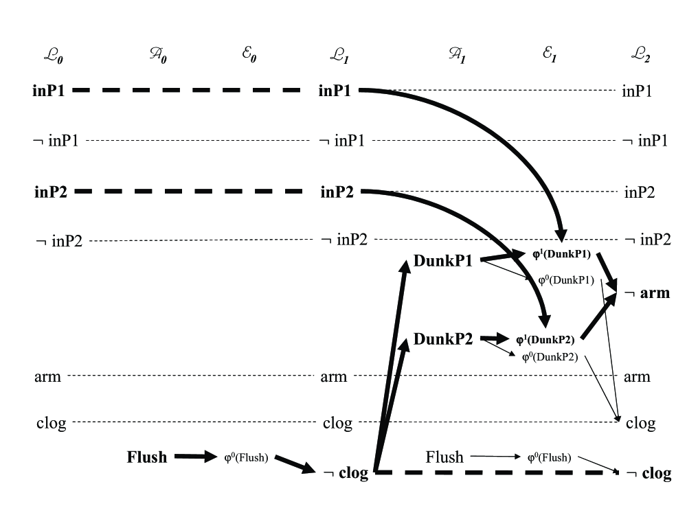
Figure 7: The $LUG$ skeleton for CBTC, with no mutexes. The relaxed plan for $h^{LUG}_{RP}$ is shown in bold.

Initial Literal Layer: The $LUG$ has an initial layer consisting of every literal with a non false ($\perp$) label. In the initial layer the label $\ell_{0}(l)$ of each literal $l$ is identical to $l\wedge BS_{P}$, representing the states of $BS_{P}$ in which $l$ holds. The labels for the initial layer literals are propagated through actions and effects to label the next literal layer, as we will describe shortly. We continue propagation until no label of any literal changes between layers, a condition referred to as “level off”.

The $LUG$ for CBTC, shown in Figure 7 (without labels), using $BS_{P}$=$BS_{I}$ has the initial literal layer:

$$\begin{array}[]{l}{\cal L}_{0}=\{{\tt inP1},\neg{\tt inP2},{\tt inP2},\neg{\tt inP1},{\tt clog},{\tt arm}\}\\ \ell_{0}({\tt inP1})=\ell_{0}(\neg{\tt inP2})=({\tt arm}\wedge{\tt clog}\wedge{\tt inP1}\wedge\neg{\tt inP2}),\\ \ell_{0}({\tt inP2})=\ell_{0}(\neg{\tt inP1})=({\tt arm}\wedge{\tt clog}\wedge\neg{\tt inP1}\wedge{\tt inP2}),\\ \ell_{0}({\tt clog})=\ell_{0}({\tt arm})=BS_{P}\end{array}$$

Notice that inP1 and inP2 have labels indicating the respective initial states in which they hold, and clog and arm have $BS_{P}$ as their label because they hold in all states in $BS_{P}$.

Action Layer: Once the previous literal layer ${\cal L}_{k}$ is computed, we construct and label the action layer ${\cal A}_{k}$. ${{\cal A}}_{k}$ contains causative actions from the action set $A$, plus literal persistence. An action is included in ${{\cal A}}_{k}$ if its label is not false (i.e. $\ell_{k}(a)\not=\perp$). The label of an action at level $k$, is equivalent to the extended label of its execution precondition:

$$\ell_{k}(a)=\ell^{*}_{k}(\rho^{e}(a))$$

Above, we introduce the notation for extended labels $\ell_{k}^{*}(f)$ of a formula $f$ to denote the worlds of $BS_{P}$ that can reach $f$ at level $k$. We say that any propositional formula $f$ is reachable from $BS$ after $k$ levels if $BS_{i}\models\ell^{*}_{k}(f)$. Since we only have labels for literals, we substitute the labels of literals for the literals in a formula to get the extended label of the formula. The extended label of a propositional formula $f$ at level $k$, is defined:

$$\begin{array}[]{c}\ell^{*}_{k}(f\wedge f^{\prime})=\ell^{*}_{k}(f)\wedge\ell^{*}_{k}(f^{\prime}),\\ \ell^{*}_{k}(f\vee f^{\prime})=\ell^{*}_{k}(f)\vee\ell^{*}_{k}(f^{\prime}),\\ \ell^{*}_{k}(\neg(f\wedge f^{\prime}))=\ell^{*}_{k}(\neg f\vee\neg f^{\prime}),\\ \ell^{*}_{k}(\neg(f\vee f^{\prime}))=\ell^{*}_{k}(\neg f\wedge\neg f^{\prime}),\\ \ell^{*}_{k}(\top)=BS_{P},\\ \ell^{*}_{k}(\perp)=\perp,\\ \ell^{*}_{k}(l)=\ell_{k}(l)\\ \end{array}$$

The zeroth action layer for CBTC is:

$$\begin{array}[]{l}{{\cal A}}_{0}=\{{\tt Flush},{\tt inP1}_{p},\neg{\tt inP2}_{p},{\tt inP2}_{p},\neg{\tt inP1}_{p},{\tt clog}_{p},{\tt arm}_{p}\}\\ \ell_{0}({\tt Flush})=BS_{P},\\ \ell_{0}({\tt inP1}_{p})=\ell_{0}(\neg{\tt inP2}_{p})=({\tt arm}\wedge{\tt clog}\wedge{\tt inP1}\wedge\neg{\tt inP2}),\\ \ell_{0}({\tt inP2}_{p})=\ell_{0}(\neg{\tt inP1}_{p})=({\tt arm}\wedge{\tt clog}\wedge\neg{\tt inP1}\wedge{\tt inP2}),\\ \ell_{0}({\tt clog}_{p})=\ell_{0}({\tt arm}_{p})=BS_{P}\end{array}$$

Each literal persistence has a label identical to the label of the corresponding literal from the previous literal layer. The Flush action has $BS_{P}$ as its label because it is always applicable.

Effect Layer: The effect layer ${{\cal E}}_{k}$ depends both on the literal layer ${\cal L}_{k}$ and action layer ${\cal A}_{k}$. ${{\cal E}}_{k}$ contains an effect $\varphi^{j}(a)$ if the effect has a non false label (i.e. $\ell_{k}(\varphi^{j}(a))\not=\perp$). Because both the action and an effect must be applicable in the same world, the label of the effect at level $k$ is the conjunction of the label of the associated action with the extended label of the antecedent

$$\ell_{k}(\varphi^{j}(a))=\ell_{k}(a)\wedge\ell^{*}_{k}(\rho^{j}(a))$$

The zeroth effect layer for CBTC is:

$$\begin{array}[]{l}{{\cal E}}_{0}=\{\varphi^{0}({\tt Flush}),\varphi^{0}({\tt inP1}_{p}),\varphi^{0}(\neg{\tt inP2}_{p}),\varphi^{0}({\tt inP2}_{p}),\\ \qquad\;\;\,\varphi^{0}(\neg{\tt inP1}_{p}),\varphi^{0}({\tt clog}_{p}),\varphi^{0}({\tt arm}_{p})\}\\ \ell_{0}(\varphi^{0}({\tt Flush}))=BS_{P}\\ \ell_{0}(\varphi^{0}({\tt inP1}_{p}))=\ell_{0}(\varphi^{0}(\neg{\tt inP2}_{p}))=({\tt arm}\wedge{\tt clog}\wedge{\tt inP1}\wedge\neg{\tt inP2}),\\ \ell_{0}(\varphi^{0}({\tt inP2}_{p}))=\ell_{0}(\varphi^{0}(\neg{\tt inP1}_{p}))=({\tt arm}\wedge{\tt clog}\wedge\neg{\tt inP1}\wedge{\tt inP2}),\\ \ell_{0}(\varphi^{0}({\tt clog}_{p}))=\ell_{0}(\varphi^{0}({\tt arm}_{p}))=BS_{P}\end{array}$$

Again, like the action layer, the unconditional effect of each literal persistence has a label identical to the corresponding literal in the previous literal layer. The unconditional effect of Flush has a label identical to the label of Flush.

Literal Layer: The literal layer ${\cal L}_{k}$ depends on the previous effect layer ${\cal E}_{k-1}$, and contains only literals with non false labels (i.e. $\ell_{k}(l)\not=\perp$). An effect $\varphi^{j}(a)\in{\cal E}_{k-1}$ contributes to the label of a literal $l$ when the effect consequent contains the literal $l$. The label of a literal is the disjunction of the labels of each effect from the previous effect layer that gives the literal:

$$\ell_{k}(l)=\bigvee_{\begin{subarray}{c}\varphi^{j}(a):l\in\varepsilon^{j}(a),\\ \varphi^{j}(a)\in{\cal E}_{k-1}\end{subarray}}\ell_{k-1}(\varphi^{j}(a))$$

The first literal layer for CBTC is:

$$\begin{array}[]{l}{\cal L}_{1}=\{{\tt inP1},\neg{\tt inP2},{\tt inP2},\neg{\tt inP1},\neg{\tt clog},{\tt clog},{\tt arm}\}\\ \ell_{1}({\tt inP1})=\ell_{1}(\neg{\tt inP2})=({\tt arm}\wedge{\tt clog}\wedge{\tt inP1}\wedge\neg{\tt inP2}),\\ \ell_{1}({\tt inP2})=\ell_{1}(\neg{\tt inP1})=({\tt arm}\wedge{\tt clog}\wedge\neg{\tt inP1}\wedge{\tt inP2}),\\ \ell_{1}(\neg{\tt clog})=\ell_{1}({\tt clog})=\ell_{1}({\tt arm})=BS_{P}\end{array}$$

This literal layer is identical to the initial literal layer, except that $\neg$clog goes from having a false label (i.e. not existing in the layer) to having the label $BS_{P}$.

We continue to the level one action layer because ${\cal L}_{1}$ does not indicate that $BS_{G}$ is reachable from $BS_{P}$ ($\neg$arm $\not\in{\cal L}_{1}$). Action layer one is defined:

$$\begin{array}[]{l}{{\cal A}}_{1}=\{{\tt DunkP1},{\tt DunkP2},{\tt Flush},{\tt inP1}_{p},\neg{\tt inP2}_{p},{\tt inP2}_{p},\neg{\tt inP1}_{p},{\tt clog}_{p},{\tt arm}_{p},\neg{\tt clog}_{p}\}\\ \ell_{1}({\tt DunkP1})=\ell_{1}({\tt DunkP2})=\ell_{1}({\tt Flush})=BS_{P},\\ \ell_{1}({\tt inP1}_{p})=\ell_{1}(\neg{\tt inP2}_{p})=({\tt arm}\wedge{\tt clog}\wedge{\tt inP1}\wedge\neg{\tt inP2}),\\ \ell_{1}({\tt inP2}_{p})=\ell_{1}(\neg{\tt inP1}_{p})=({\tt arm}\wedge{\tt clog}\wedge\neg{\tt inP1}\wedge{\tt inP2}),\\ \ell_{1}({\tt clog}_{p})=\ell_{1}({\tt arm}_{p})=\ell_{1}(\neg{\tt clog}_{p})=BS_{P}\end{array}$$

This action layer is similar to the level zero action layer. It adds both Dunk actions because they are now executable. We also add the persistence for $\neg$clog. Each Dunk action gets a label identical to its execution precondition label.

The level one effect layer is:

$$\begin{array}[]{l}{{\cal E}}_{1}=\{\varphi^{0}({\tt DunkP1}),\varphi^{0}({\tt DunkP2}),\varphi^{1}({\tt DunkP1}),\varphi^{1}({\tt DunkP2}),\varphi^{0}({\tt Flush}),\varphi^{0}({\tt inP1}_{p}),\\ \qquad\;\;\,\varphi^{0}(\neg{\tt inP2}_{p}),\varphi^{0}({\tt inP2}_{p}),\varphi^{0}(\neg{\tt inP1}_{p}),\varphi^{0}({\tt clog}_{p}),\varphi^{0}({\tt arm}_{p}),\varphi^{0}(\neg{\tt clog}_{p})\}\\ \ell_{1}(\varphi^{0}({\tt DunkP1}))=\ell_{1}(\varphi^{0}({\tt DunkP2}))=\ell_{1}(\varphi^{0}({\tt Flush}))=BS_{P}\\ \ell_{1}(\varphi^{1}({\tt DunkP1}))=({\tt arm}\wedge{\tt clog}\wedge{\tt inP1}\wedge\neg{\tt inP2}),\\ \ell_{1}(\varphi^{1}({\tt DunkP2}))=({\tt arm}\wedge{\tt clog}\wedge\neg{\tt inP1}\wedge{\tt inP2}),\\ \ell_{1}(\varphi^{0}(\neg{\tt inP2}_{p}))=\ell_{1}(\varphi^{0}({\tt inP1}_{p}))=({\tt arm}\wedge{\tt clog}\wedge{\tt inP1}\wedge\neg{\tt inP2}),\\ \ell_{1}(\varphi^{0}(\neg{\tt inP1}_{p}))=\ell_{1}(\varphi^{0}({\tt inP2}_{p}))=({\tt arm}\wedge{\tt clog}\wedge\neg{\tt inP1}\wedge{\tt inP2}),\\ \ell_{1}(\varphi^{0}({\tt clog}_{p}))=\ell_{1}(\varphi^{0}({\tt arm}_{p}))=\ell_{1}(\varphi^{0}(\neg{\tt clog}_{p}))=BS_{P}\end{array}$$

The conditional effects of the Dunk actions in CBTC (Figure 7) have labels that indicate the possible worlds in which they will give $\neg$arm because their antecedents do not hold in all possible worlds. For example, the conditional effect $\varphi^{1}($DunkP1$)$ has the label found by taking the conjunction of the action’s label $BS_{P}$ with the antecedent label $\ell^{*}_{1}$(inP1) to obtain $({\tt arm}\wedge{\tt clog}\wedge{\tt inP1}\wedge\neg{\tt inP2})$.

Finally, the level two literal layer:

$$\begin{array}[]{l}{\cal L}_{2}=\{{\tt inP1},\neg{\tt inP2},{\tt inP2},\neg{\tt inP1},\neg{\tt clog},{\tt clog},{\tt arm},\neg{\tt arm}\}\\ \ell_{2}({\tt inP1})=\ell_{2}(\neg{\tt inP2})=({\tt arm}\wedge{\tt clog}\wedge{\tt inP1}\wedge\neg{\tt inP2}),\\ \ell_{2}({\tt inP2})=\ell_{2}(\neg{\tt inP1})=({\tt arm}\wedge{\tt clog}\wedge\neg{\tt inP1}\wedge{\tt inP2}),\\ \ell_{2}(\neg{\tt clog})=\ell_{2}({\tt clog})=\ell_{2}({\tt arm})=\ell_{2}(\neg{\tt arm})=BS_{P}\end{array}$$

The labels of the literals for level 2 of CBTC indicate that $\neg$arm is reachable from $BS_{P}$ because its label is entailed by $BS_{P}$. The label of $\neg$arm is found by taking the disjunction of the labels of effects that give it, namely, $({\tt arm}\wedge{\tt clog}\wedge{\tt inP1}\wedge\neg{\tt inP2})$ from the conditional effect of DunkP1 and $({\tt arm}\wedge{\tt clog}\wedge\neg{\tt inP1}\wedge{\tt inP2})$ from the conditional effect of DunkP2, which reduces to $BS_{P}$. Construction could stop here because $BS_{P}$ entails the label of the goal $\ell^{*}_{k}(\neg$arm$\wedge\neg$clog)$=\ell_{k}(\neg$arm$)\wedge\ell_{k}(\neg$clog$)=BS_{P}\wedge BS_{P}=BS_{P}$. However, level off occurs at the next level because there is no change in the labels of the literals.

When level off occurs at level three in our example, we can say that for any $BS$, where $BS\models BS_{P}$, that a formula $f$ is reachable in $k$ steps if $BS\models\ell^{*}_{k}(f)$. If no such level $k$ exists, then $f$ is not reachable from $BS$. If there is some level $k$, where $f$ is reachable from $BS$, then the first such $k$ is a lower bound on the number of parallel plan steps needed to reach $f$ from $BS$. This lower bound is similar to the classical planning max heuristic (?). We can provide a more informed heuristic by extracting a relaxed plan to support $f$ with respect to $BS$, described shortly.

4.4.2 Same-World Labelled Mutexes

There are several types of mutexes that can be added to the $LUG$. To start with, we only concentrate on those that can evolve in a single possible world because same-world mutexes are more effective as well as relatively easy to understand. We extend the mutex propagation that was used in the multiple graphs so that the mutexes are on one planning graph. The savings of computing mutexes on the $LUG$ instead of multiple graphs is that we can reduce computation when a mutex exits in several worlds. In Appendix B we describe how to handle cross-world mutexes, despite their lack of effectiveness in the experiments we conducted. Cross-world mutexes extend the $LUG$ to compute the same set of mutexes found by CGP (?).

Same-world mutexes can be represented with a single label, $\hat{\ell}_{k}(x_{1},x_{2})$, between two elements (actions, effect, or literals). The mutex holds between elements $x_{1}$ and $x_{2}$ in all worlds $S$ where $S\models\hat{\ell}_{k}(x_{1},x_{2})$. If the elements are not mutex in any world, we can assume the label of a mutex between them is false $\perp$. We discuss how the labelled mutexes are discovered and propagated for actions, effect relations, and literals.

By using mutexes, we can refine what it means for a formula $f$ to be reachable from a set of worlds $BS_{P}$. We must ensure that for every state in $BS_{P}$, there exists a state of $f$ that is reachable. A state $S^{\prime}$ of $f$ is reachable from a state $S$ of $BS_{P}$ when there are no two literals in $S^{\prime}$ that are mutex in world $S$ and $BS_{P}\models\ell_{k}^{*}(S)$.

In each of the action, effect, and literal layers there are multiple ways for the same pair of elements to become mutex (e.g. interference or competing needs). Thus, the mutex label for a pair is the disjunction of all labelled mutexes found for the pair by some means.

Action Mutexes: The same-world action mutexes at a level $k$ are a set of labelled pairs of actions. Each pair is labelled with a formula that indicates the set of possible worlds where the actions are mutex. The possible reasons for mutex actions are interference and competing needs.

• Interference Two actions $a,a^{\prime}$ interfere if (1) the unconditional effect consequent $\varepsilon^{0}(a)$ of one is inconsistent with the execution precondition $\rho^{e}(a^{\prime})$ of the other, or (2) vice versa. They additionally interfere if (3) both unconditional effect consequents $\varepsilon^{0}(a)$ and $\varepsilon^{0}(a^{\prime})$ are inconsistent, or (4) both execution preconditions $\rho^{e}(a)$ and $\rho^{e}(a^{\prime})$ are inconsistent. The mutex will exist in all possible world projections $\hat{\ell}_{k}(a,a^{\prime})=BS_{P}$. Formally, $a$ and $a^{\prime}$ interfere if one of the following holds:

  $$\begin{array}[]{l}{\tt(1)}\;\varepsilon^{0}(a)\wedge\rho^{e}(a^{\prime})=\perp\\ {\tt(2)}\;\rho^{e}(a)\wedge\varepsilon^{0}(a^{\prime})=\perp\\ {\tt(3)}\;\varepsilon^{0}(a)\wedge\varepsilon^{0}(a^{\prime})=\perp\\ {\tt(4)}\;\rho^{e}(a)\wedge\rho^{e}(a^{\prime})=\perp\end{array}$$

• Competing Needs Two actions $a,a^{\prime}$ have competing needs in a world when a pair of literals from their execution preconditions are mutex in the world. The worlds where $a$ and $a^{\prime}$ are mutex because of competing needs are described by:

  $$\ell_{k}(a)\wedge\ell_{k}(a^{\prime})\wedge\bigvee_{\begin{subarray}{c}l\in\rho^{j}(a),l^{\prime}\in\rho^{j}(a^{\prime})\end{subarray}}\hat{\ell}_{k}(l,l^{\prime})$$

  In the above formula we find all worlds where a pair of execution preconditions $l\in\rho^{e}(a),l^{\prime}\in\rho^{e}(a^{\prime})$ are mutex and both actions are reachable.

Effect Mutexes: The effect mutexes are a set of labelled pairs of effects. Each pair is labelled with a formula that indicates the set of possible worlds where the effects are mutex. The possible reasons for mutex effects are associated action mutexes, interference, competing needs, or induced effects.

• Mutex Actions Two effects $\varphi^{i}(a)\in\Phi(a),\varphi^{j}(a^{\prime})\in\Phi({a^{\prime}})$ are mutex in all worlds where their associated actions are mutex, $\hat{\ell}_{k}(a,a^{\prime})$.

• Interference Like actions, two effects $\varphi^{i}(a),\varphi^{j}(a^{\prime})$ interfere if (1) the consequent $\varepsilon^{i}(a)$ of one is inconsistent with the antecedent $\rho^{j}(a^{\prime})$ of the other, or (2) vice versa. They additionally interfere if (3) both effect consequents $\varepsilon^{i}(a)$ and $\varepsilon^{j}(a^{\prime})$ are inconsistent, or (4) both antecedents $\rho^{i}(a)$ and $\rho^{j}(a^{\prime})$ are inconsistent. The mutex will exist in all possible world projections, so the label of the mutex is $\hat{\ell}_{k}(\varphi^{i}(a),\varphi^{j}(a^{\prime}))=BS_{P}$. Formally, $\varphi^{i}(a)$ and $\varphi^{j}(a^{\prime})$ interfere if one of the following holds:

  $$\begin{array}[]{l}{\tt(1)}\;\varepsilon^{i}(a)\wedge\rho^{j}(a^{\prime})=\perp\\ {\tt(2)}\;\rho^{i}(a)\wedge\varepsilon^{j}(a^{\prime})=\perp\\ {\tt(3)}\;\varepsilon^{i}(a)\wedge\varepsilon^{j}(a^{\prime})=\perp\\ {\tt(4)}\;\rho^{i}(a)\wedge\rho^{j}(a^{\prime})=\perp\end{array}$$

• Competing Needs Like actions, two effects have competing needs in a world when a pair of literals from their antecedents are mutex in a world. The worlds where $\varphi^{i}(a)$ and $\varphi^{j}(a^{\prime})$ have a competing needs mutex are:

  $$\ell_{k}(\varphi^{i}(a))\wedge\ell_{k}(\varphi^{j}(a^{\prime}))\wedge\bigvee_{\begin{subarray}{c}l\in\rho^{i}(a),l^{\prime}\in\rho^{j}(a^{\prime})\end{subarray}}\hat{\ell}_{k}(l,l^{\prime})$$

  In the above formula we find all worlds where a pair of execution preconditions $l\in\rho^{i}(a),l^{\prime}\in\rho^{j}(a^{\prime})$ are mutex and both actions are reachable.

• Induced An induced effect $\varphi^{j}(a)$ of an effect $\varphi^{i}(a)$ is an effect of the same action $a$ that may execute at the same time. An effect is induced by another in the possible worlds where they are both reachable. For example, the conditional effect of an action always induces the unconditional effect of the action.

  Induced mutexes, involving the inducing effect $\varphi^{i}(a)$, come about when an induced effect $\varphi^{j}(a)$ is mutex with another effect $\varphi^{h}(a^{\prime})$ (see Figure 8). The induced mutex is between (a) the effect $\varphi^{h}(a^{\prime})$ that is mutex with the induced effect $\varphi^{j}(a)$ and (b) the inducing effect $\varphi^{i}(a)$. The label of the mutex is the conjunction of the label of the mutex $\hat{\ell_{k}}(\varphi^{j}(a),\varphi^{h}(a^{\prime}))$ and the label of the induced effect $\varphi^{j}(a)$. For additional discussion of the methodology behind induced mutexes we refer to ? (?).

  

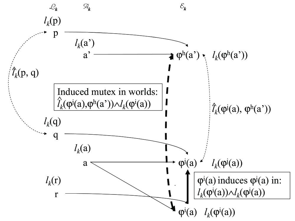
  Figure 8: Effect $\varphi^{i}(a)$ induces effect $\varphi^{j}(a)$. $\varphi^{j}(a)$ is mutex with $\varphi^{h}(a^{\prime})$, so $\varphi^{i}(a)$ is induced mutex with $\varphi^{h}(a^{\prime})$.

Literal Mutexes: The literal mutexes are a set of labelled pairs of literals. Each pair is labelled with a formula that indicates the set of possible worlds where the literals are mutex. The only reason for mutex literals is inconsistent support.

• Inconsistent Support Two literals have inconsistent support in a possible world at level $k$ when there are no two non-mutex effects that support both literals in the world. The label of the literal mutex at level $k$ is a disjunction of all worlds where they have inconsistent support. The worlds for an inconsistent support mutex between $l$ and $l^{\prime}$ are:

  $$\bigvee_{\begin{subarray}{c}S:\forall\varphi^{i}(a),\varphi^{j}(a^{\prime})\in{\cal E}_{k-1},\\ {\tt where}\,l\in\varepsilon^{i}(a),l^{\prime}\in\varepsilon^{j}(a^{\prime}),\\ S\models\hat{\ell}_{k-1}(\varphi^{i}(a),\varphi^{j}(a^{\prime}))\end{subarray}}S$$

  The meaning of the above formula is that the two literals are mutex in all worlds $S$ where all pairs of effects that support the literals in $S$ are mutex in $S$.

4.4.3 $LUG$ Heuristics

The heuristics computed on the $LUG$ can capture measures similar to the $MG$ heuristics, but there exists a new opportunity to make use of labels to improve heuristic computation efficiency. A single planning graph is sufficient if there is no state aggregation being measured, so we do not mention such measures for the $LUG$.

Positive Interaction Aggregation: Unlike $MG$ heuristics, we do not compute positive interaction based relaxed plans on the $LUG$. The $MG$ approach to measure positive interaction across each state in a belief state is to compute multiple relaxed plans and take their maximum value. To get the same measure on the $LUG$ we would still need to extract multiple relaxed plans, the situation we are trying to avoid by using the $LUG$. While the graph construction overhead may be lowered by using the $LUG$, the heuristic computation could take too long. Hence, we do not compute relaxed plans on the $LUG$ to measure positive interaction alone, but we do compute relaxed plans that measure overlap (which measures positive interaction).

Independence Aggregation: Like positive interaction aggregation, we need a relaxed plan for every state in the projected belief state to find the summation of the costs. Hence, we do not compute relaxed plans that assume independence.

State Overlap Aggregation: A relaxed plan extracted from the $LUG$ to get the $h^{LUG}_{RP}$ heuristic resembles the unioned relaxed plan in the $h^{MG}_{RPU}$ heuristic. Recall that the $h^{MG}_{RPU}$ heuristic extracts a relaxed plan from each of the multiple planning graphs (one for each possible world) and unions the set of actions chosen at each level in each of the relaxed plans. The $LUG$ relaxed plan heuristic is similar in that it counts actions that have positive interaction in multiple worlds only once and accounts for independent actions that are used in subsets of the possible worlds. The advantage of $h^{LUG}_{RP}$ is that we find these actions with a single pass on one planning graph.

We are trading the cost of computing multiple relaxed plans for the cost of manipulating $LUG$ labels to determine what lines of causal support are used in what worlds. In the relaxed plan we want to support the goal with every state in $BS_{P}$, but in doing so we need to track which states in $BS_{P}$ use which paths in the planning graph. A subgoal may have several different (and possibly overlapping) paths from the worlds in $BS_{P}$.

A $LUG$ relaxed plan is a set of layers: $\{{\cal A}^{RP}_{0},{\cal E}^{RP}_{0},{\cal L}^{RP}_{1},...,$ ${\cal A}^{RP}_{b-1},{\cal E}^{RP}_{b-1},$ ${\cal L}^{RP}_{b}\}$, where ${\cal A}^{RP}_{r}$ is a set of actions, ${\cal E}^{RP}_{r}$ is a set of effects, and ${\cal L}^{RP}_{r+1}$ is a set of clauses. The elements of the layers are labelled to indicate the worlds of $BS_{P}$ where they are chosen for support. The relaxed plan is extracted from the level $b=h^{LUG}_{level}(BS_{i})$ (i.e., the first level where $BS_{i}$ is reachable, also described in Appendix A).

Please note that we are extracting the relaxed plan for $BS_{i}$ in terms of clauses, and not literals, which is different than the $SG$ and $MG$ versions of relaxed plans. Previously we found the constituent of $BS_{i}$ that was first reached on a planning graph and now we do not commit to any one constituent. Our rationale is that we were possibly using different constituents in each of the multiple graphs, and in this condensed version of the multiple graphs we still want to be able to support different constituents of the $BS_{i}$ in different worlds. We could also use the constituent representation of $BS_{i}$ in defining the layers of the relaxed plan, but choose the clausal representation of $BS_{i}$ instead because we know that we have to support each clause. However with constituents we know we only need to support one (but we don’t need to know which one).

The relaxed plan, shown in bold in Figure 7, for $BS_{I}$ to reach $BS_{G}$ in CBTC is listed as follows:

$$\noindent\begin{array}[]{l}{\cal A}^{RP}_{0}=\{{\tt inP1}_{p},{\tt inP2}_{p},{\tt Flush}\},\\ \quad\ell^{RP}_{0}({\tt inP1}_{p})=({\tt arm}\wedge\neg{\tt clog}\wedge{\tt inP1}\wedge\neg{\tt inP2}),\\ \quad\ell^{RP}_{0}({\tt inP2}_{p})=({\tt arm}\wedge\neg{\tt clog}\wedge\neg{\tt inP1}\wedge{\tt inP2}),\\ \quad\ell^{RP}_{0}({\tt Flush})=BS_{P},\\ \\ {\cal E}^{RP}_{0}=\{\varphi^{0}({\tt inP1}_{p}),\varphi^{0}({\tt inP2}_{p}),\varphi^{0}({\tt Flush})\},\\ \quad\ell^{RP}_{0}(\varphi^{0}({\tt inP1}_{p}))=({\tt arm}\wedge\neg{\tt clog}\wedge{\tt inP1}\wedge\neg{\tt inP2}),\\ \quad\ell^{RP}_{0}(\varphi^{0}({\tt inP2}_{p}))=({\tt arm}\wedge\neg{\tt clog}\wedge\neg{\tt inP1}\wedge{\tt inP2}),\\ \quad\ell^{RP}_{0}(\varphi^{0}({\tt Flush}))=BS_{P},\\ \\ {\cal L}^{RP}_{1}=\{{\tt inP1},{\tt inP2},\neg{\tt clog}\},\\ \quad\ell^{RP}_{1}({\tt inP1})=({\tt arm}\wedge\neg{\tt clog}\wedge{\tt inP1}\wedge\neg{\tt inP2}),\\ \quad\ell^{RP}_{1}({\tt inP2})=({\tt arm}\wedge\neg{\tt clog}\wedge\neg{\tt inP1}\wedge{\tt inP2}),\\ \quad\ell^{RP}_{1}(\neg{\tt clog})=BS_{P},\\ \\ {\cal A}^{RP}_{1}=\{{\tt DunkP1},{\tt DunkP2},\neg{\tt clog}_{p}\},\\ \quad\ell^{RP}_{1}({\tt DunkP1})=({\tt arm}\wedge\neg{\tt clog}\wedge{\tt inP1}\wedge\neg{\tt inP2}),\\ \quad\ell^{RP}_{1}({\tt DunkP2})=({\tt arm}\wedge\neg{\tt clog}\wedge\neg{\tt inP1}\wedge{\tt inP2}),\\ \quad\ell^{RP}_{1}(\neg{\tt clog}_{p})=BS_{P},\\ \\ {\cal E}^{RP}_{1}=\{\varphi^{1}({\tt DunkP1}),\varphi^{1}({\tt DunkP2}),\varphi^{0}(\neg{\tt clog}_{p})\},\\ \quad\ell^{RP}_{1}(\varphi^{1}({\tt DunkP1}))=({\tt arm}\wedge\neg{\tt clog}\wedge{\tt inP1}\wedge\neg{\tt inP2}),\\ \quad\ell^{RP}_{1}(\varphi^{1}({\tt DunkP2}))=({\tt arm}\wedge\neg{\tt clog}\wedge\neg{\tt inP1}\wedge{\tt inP2}),\\ \quad\ell^{RP}_{1}(\varphi^{0}(\neg{\tt clog}_{p}))=BS_{P},\\ \\ {\cal L}^{RP}_{2}=\{\neg{\tt arm},\neg{\tt clog}\},\\ \quad\ell^{RP}_{2}(\neg{\tt arm})=BS_{P},\\ \quad\ell^{RP}_{2}(\neg{\tt clog})=BS_{P}\\ \end{array}$$

We start by forming ${\cal L}_{2}^{RP}$ with the clauses in $\kappa(BS_{G})$, namely $\neg$arm and $\neg$clog; we label the clauses with $BS_{P}$ because they need to be supported by all states in our belief state. Next, we support each clause in ${\cal L}_{2}^{RP}$ with the relevant effects from ${\cal E}_{1}$ to form ${\cal E}_{1}^{RP}$. For $\neg$clog we use persistence because it supports $\neg$clog in all worlds described by $BS_{P}$ (this is an example of positive interaction of worlds). For $\neg$arm the relevant effects are the respective $\varphi^{1}$ from each Dunk action. We choose both effects to support $\neg$arm because we need to support $\neg$arm in all worlds of $BS_{P}$, and each effect gives support in only one world (this is an example of independence of worlds). We then insert the actions associated with each chosen effect into ${\cal A}_{1}^{RP}$ with the appropriate label indicating the worlds where it was needed, which in general is fewer worlds than where it is reachable (i.e. it is always the case that $\ell^{RP}_{r}(\cdot)\models\ell_{r}(\cdot)$). Next we form ${\cal L}_{1}^{RP}$ with the execution preconditions of actions in ${\cal A}_{1}^{RP}$ and antecedents of effects in ${\cal E}_{1}^{RP}$, which are $\neg$clog, inP1, and inP2, labelled with all worlds where an action or effect needed them. In the same fashion as level two, we support the literals at level one, using persistence for inP1 and inP2, and Flush for $\neg$clog. We stop here, because we have supported all clauses at level one.

For the general case, extraction starts at the level $b$ where $BS_{i}$ is first reachable from $BS_{P}$. The first relaxed plan layers we construct are ${\cal A}^{RP}_{b-1},{\cal E}^{RP}_{b-1},{\cal L}^{RP}_{b}$, where ${\cal L}^{RP}_{b}$ contains all clauses $C\in\kappa(BS_{i})$, labelled as $\ell^{RP}_{k}(C)=BS_{P}$.

For each level $r$, $1\leq r\leq b$, we support each clause in ${\cal L}^{RP}_{r}$ by choosing relevant effects from ${\cal E}_{r-1}$ to form ${\cal E}^{RP}_{r-1}$. An effect $\varphi^{j}(a)$ is relevant if it is reachable in some of the worlds where we need to support $C$ (i.e. $\ell_{r-1}(\varphi^{j}(a))\wedge\ell^{RP}_{r}(C)\not=\perp$) and the consequent gives a literal $l\in C$. For each clause, we have to choose enough supporting effects so that the chosen effect worlds are a superset of the worlds we need to support the clause, formally:

$$\forall_{C\in{\cal L}^{RP}_{r}}\ell^{RP}_{r}(C)\models\left(\bigvee_{\begin{subarray}{c}\varphi^{j}(a):l\in\varepsilon^{j}(a),\\ l\in C,\\ \varphi^{j}(a)\in{\cal E}_{r-1}\end{subarray}}\ell_{r-1}^{RP}(\varphi^{j}(a))\right)$$

We think of supporting a clause in a set of worlds as a set cover problem where effects cover subsets of worlds. Our algorithm to cover the worlds of a clause with worlds of effects is a variant of the well known greedy algorithm for set cover (?). We first choose all relevant persistence effects that can cover worlds, then choose action effects that cover the most new worlds. Each effect we choose for support is added to ${\cal E}^{RP}_{r-1}$ and labelled with the new worlds it covered for $C$. Once all clauses in ${\cal L}^{RP}_{r}$ are covered, we form the action layer ${\cal A}^{RP}_{r-1}$ as all actions that have an effect in ${\cal E}^{RP}_{r-1}$. The actions in ${\cal A}^{RP}_{r-1}$ are labelled to indicate all worlds where any of their effects were labelled in ${\cal E}^{RP}_{r-1}$.

We obtain the next subgoal layer, ${\cal L}^{RP}_{r-1}$, by adding literals from the execution preconditions of actions in ${\cal A}^{RP}_{r-1}$ and antecedents of effects in ${\cal E}^{RP}_{r-1}$. Each literal $l\in{\cal L}^{RP}_{r-1}$ is labelled to indicate all worlds where any action or effect requires $l$. We support the literals in ${\cal L}^{RP}_{r-1}$ in the same fashion as ${\cal L}^{RP}_{r}$. We continue to support literals with effects, insert actions, and insert action and effect preconditions until we have supported all literals in ${\cal L}^{RP}_{1}$.

Once we get a relaxed plan, the relaxed plan heuristic, $h_{RP}^{LUG}(BS_{i})$, is the summation of the number of actions in each action layer, formally:

$$h^{LUG}_{RP}(BS_{i})=\sum\limits_{i=0}^{b-1}\mid{{\cal A}^{RP}_{i}}\mid$$

Thus in our CBTC example we have $h^{LUG}_{RP}(BS_{G})=3$. Notice that if we construct the $LUG$ without mutexes for CBTC we reach the goal after two layers. If we had included mutexes the $LUG$, then it would reach the goal after three layers. The way we use mutexes will not change our relaxed plan because we do not use mutexes to influence relaxed plan extraction. Mutexes only help to identify when a the belief state $BS_{i}$ is not reachable from $BS_{P}$.

5 Empirical Evaluation: Setup

This section presents our implementation of the ${\cal C}{\sl AltAlt}$ and $POND$ planners and the domains we use in the experiments. All tests were run in Linux on an x86 machine with a 2.66GHz P4 processor and 1GB RAM with a timeout of 20 minutes. Both CAltAlt and $POND$ used a heuristic weight of five in the, respective, A* and AO* searches. We compare with the competing approaches (CGP, SGP, GPT v1.40, MBP v0.91, KACMBP, YKA, and CFF) on several domains and problems. Our planners and all domain and problem files for all of the compared planners can be found in the online appendix.

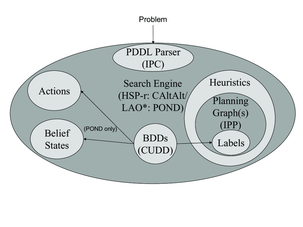
Figure 9: The implementations of CAltAlt and $POND$ rely on many existing technologies. The search engine is guided by heuristics extracted from planning graphs.

5.1 Implementation

The implementation of CAltAlt uses several off-the-shelf planning software packages. Figure 9 shows a diagram of the system architecture for CAltAlt and $POND$. While CAltAlt extends the name of $AltAlt$, it relies on a limited subset of the implementation. The components of CAltAlt are the IPC parser for PDDL 2.1 (slightly extended to allow uncertain initial conditions), the HSP-r search engine (?), the IPP planning graph (?), and the CUDD BDD package (?) to implement the $LUG$ labels. The custom parts of the implementation include the action representation, belief state representation, regression operator, and the heuristic calculation.

The implementation of $POND$ is very similar to CAltAlt aside from the search engine, and state and action representation. $POND$ also uses the IPP source code for planning graphs. $POND$ uses modified LAO* (?) source code from Eric Hansen to perform AO* search, and CUDD (?) to represent belief states and actions. Even with deterministic actions it is possible to obtain cycles from actions with observations because we are planning in belief space. $POND$ constructs the search graph as a directed acyclic graph by employing a cycle-checking algorithm. If adding a hyper-edge to the search graph creates a cycle, then the hyper-edge cannot represent an action in a strong plan and is hence not added to the graph.

5.2 Domains

Table 2 shows some of the relative features of the different problems we used to evaluate our approach. The table shows the number of initial states, goal literals, fluents, actions, and optimal plan lengths. This can be used as a guide to gauge the difficulty of the problems, as well as our performance.

Problem	Initial	Goal	Fluents	Causative	Observational	Optimal	Optimal
	States	Literals		Actions	Actions	Parallel	Serial
Rovers1	1	1	66	88	0 {12}	5 {5}	5 {5}
Rovers2	2	1	66	88	0 {12}	8 {7}	8 {7}
Rovers3	3	1	66	88	0 {12}	10 {?}	10 {8}
Rovers4	4	1	66	88	0 {12}	13 {?}	13 {10}
Rovers5	16	3	71	97	0 {12}	? {?}	20 {?}
Rovers6	12	3	119	217	0 {18}	? {?}	? {?}
Logistics1	2	1	29	70	0 {10}	6 {6}	9 {7}
Logistics2	4	2	36	106	0 {20}	6 {?}	15 {12}
Logistics3	2	1	58	282	0 {21}	8 {?}	11 {8}
Logistics4	4	2	68	396	0 {42}	8 {?}	18 {?}
Logistics5	8	3	78	510	0 {63}	? {?}	28 {?}
BT($n$)	$n$	1	$n$+1	$n$	0 {$n$}	1 {1}	$n$ {$n$-1}
BTC($n$)	$n$	1	$n$+2	$n$+1	0 {$n$}	2$n$-1 {2}	2$n$-1 {$n$-1}
CubeCenter($n$)	$n$3	3	3$n$	6	0	(3$n$-3)/2	(9$n$-3)/2
Ring($n$)	$n$3n	$n$	4$n$	4	0	3$n$-1	3$n$-1

Table 2: Features of test domains and problems - Number of initial states, Number of goal literals, Number of fluents, Number of causative actions, Number of Observational Actions, Optimal number of parallel plan steps, Optimal number of serial plan steps. Data for conditional versions of domains is in braces; plan lengths for conditional plans are maximum conditional branch length.

Conformant Problems

In addition to the standard domains used in conformant planning–such as Bomb-in-the-Toilet, Ring, and Cube Center, we also developed two new domains Logistics and Rovers. We chose these new domains because they have more difficult subgoals, and have many plans of varying length.

The Ring domain involves a ring of $n$ rooms where each room is connected to two adjacent rooms. Each room has a window which can be open, closed, or locked. The goal is to have every window locked. Initially, any state is possible – we could be in any room and each window could be in any configuration. There are four actions: move right, move left, close the window in the current room, and lock the window in the current room. Closing a window only works if the window is open, and locking a window only works if the window is closed. A good conformant plan involves moving in one direction closing and locking the window in each room.

The Cube Center domain involves a three-dimensional grid (cube) where there are six actions – it is possible to move in two directions along each dimension. Each dimension consists of $n$ possible locations. Moving in a direction along which there are no more grid points leaves one in the same position. Using this phenomena, it is possible to localize in each dimension by repeatedly moving in the same direction. Initially it is possible to be at any location in the cube and the goal is to reach the center. A good conformant plan involves localizing in a corner and then moving to the center.

The Rovers domain is a conformant adaptation of the analogous domain of the classical planning track of the International Planning Competition (?). The added uncertainty to the initial state uses conditions that determine whether an image objective is visible from various vantage points due to weather, and the availability of rock and soil samples. The goal is to upload an image of an objective and some rock and soil sample data. Thus a conformant plan requires visiting all of the possible vantage points and taking a picture, plus visiting all possible locations of soil and rock samples to draw samples.

The first five Rovers problems have 4 waypoints. Problems one through four have one through four locations, respectively, at which a desired imaging objective is possibly visible (at least one will work, but we don’t know which one). Problem 5 adds some rock and soil samples as part of the goal and several waypoints where one of each can be obtained (again, we don’t know which waypoint will have the right sample). Problem 6 adds two more waypoints, keeps the same goals as Problem 5 and changes the possible locations of the rock and soil samples. In all cases the waypoints are connected in a tree structure, as opposed to completely connected.

The Logistics domain is a conformant adaptation of the classical Logistics domain where trucks and airplanes move packages. The uncertainty is the initial locations of packages. Thus, any actions relating to the movement of packages have a conditional effect that is predicated on the package actually being at a location. In the conformant version, the drivers and pilots cannot sense or communicate a package’s actual whereabouts. The problems scale by adding packages and cities.

The Logistics problems consist of one airplane, and cities with an airport, a post office, and a truck. The airplane can travel between airports and the trucks can travel within cities. The first problem has two cities and one package that could start at either post office, and the goal is to get the package to the second city’s airport. The second problem adds another package at the same possible starting points and having the same destination. The third problem has three cities with one package that could be at any post office and has to reach the third airport. The fourth problem adds a second package to the third problem with the same starting and ending locations. The fifth problem has three cities and three packages, each at one of two of the three post offices and having to reach different airports.

Conditional Problems

For conditional planning we consider domains from the literature: Bomb-in-the-Toilet with sensing BTS, and Bomb-in-the-Toilet with clogging and sensing BTCS. We also extend the conformant Logistics and Rovers to include sensory actions.

The Rovers problem allows for the rover, when it is at a particular waypoint, to sense the availability of image, soil, or rock data at that location. The locations of the collectable data are expressed as one-of constraints, so the rover can deduce the locations of collectable data by failing to sense the other possibilities.

Logistics has observations to determine if a package at a location exists, and the observation is assumed to be made by a driver or pilot at the particular location. Since there are several drivers and a pilot, different agents make the observations. The information gained by the agents is assumed to be automatically communicated to the others, as the planner is the agent that has all the knowledge.

6 Empirical Evaluation: Inter-Heuristic Comparison

We start by comparing the heuristic approaches within our planners. In the next section, we continue by describing how our planners, using the best heuristics, compare against other state of the art approaches. In this section we intend to validate our claims that belief space heuristics that measure overlap perform well across several domains. We further justify using the $LUG$ over multiple planning graphs and applying mutexes to improve heuristics in regression through pruning belief states.

We compare many techniques within CAltAlt and $POND$ on our conformant planning domains, and in addition we test the heuristics in $POND$ on the conditional domains. Our performance metrics include the total planning time and the number of search nodes expanded. Additionally, when discussing mutexes we analyze planning graph construction time. We proceed by showing how the heuristics perform in CAltAlt  and then how various mutex computation schemes for the $LUG$ can affect performance. Then we present how $POND$ performs with the different heuristics in both conformant and conditional domains, explore the effect of sampling a proportion of worlds to build $SG^{1}$, $MG$, and $LUG$ graphs, and compare the heuristic estimates in $POND$ to the optimal plan length to gauge heuristic accuracy. We finish with a summary of important conclusions.

We only compute mutexes in the planning graphs for CAltAlt because the planning graph(s) are only built once in a search episode and mutexes help prune the inconsistent belief states encountered in regression search. We abstain from computing mutexes in $POND$ because in progression we build new planning graphs for each search node and we want to keep graph computation time low. With the exception of our discussion on sampling worlds to construct the planning graphs, the planning graphs are constructed deterministically. This means that the single graph is the unioned single graph $SG^{U}$, and the $MG$ and $LUG$ graphs are built for all possible worlds.

6.1 CAltAlt

The results for CAltAlt in the conformant Rovers, Logistics, BT, and BTC domains, in terms of total time and number of expanded search nodes, are presented in Table 3. We show the number of expanded nodes because it gives an indication of how well a heuristic guides the planner. The total time captures the amount of time computing the heuristic and searching. A high total time with a high number of search nodes indicates a poor heuristic, and a high total time and low number of search nodes indicates an expensive but informed heuristic.

We do not discuss the Ring and Cube Center domains for CAltAlt because it cannot solve even the smallest instances. Due to implementation details the planner performs very poorly when domains have actions with several conditional effects and hence does not scale. The trouble stems from a weak implementation for bringing general propositional formulas (obtained by regression with several conditional effects) into CNF.

Problem	$h_{0}$	$h_{card}$	$h^{SG}_{RP}$	$h^{MG}_{m-RP}$	$h^{MG}_{RPU}$	$h^{LUG(FX)}_{RP}$
Rovers 1	2255/5	18687/14	543/5	542/5	185/5	15164/5
2	49426/8	TO	78419/8	8327/8	29285/9	32969/8
3	TO	-	91672/10	20162/10	2244/11	16668/10
4	-	-	TO	61521/16	3285/15	31584/13
5	-	-	-	TO	TO	TO
6	-	-	-	-	-	-
Logistics 1	1108/9	4268/9	198/9	183/9	1109/9	1340/9
2	TO	TO	7722/15	15491/15	69818/19	18535/15
3	-	-	3324/14	70882/14	TO	16458/15
4	-	-	141094/19	TO	-	178068/19
5	-	-	TO	-	-	TO
BT 2	19/2	14/2	18/2	20/2	21/2	12/2
10	4837/10	56/10	5158/10	8988/10	342/10	71/10
20	TO	418/20	TO	TO	2299/20	569/20
30	-	1698/30	-	-	9116/30	2517/30
40	-	5271/40	-	-	44741/40	7734/40
50	-	12859/50	-	-	TO	18389/50
60	-	26131/60	-	-	-	37820/60
70	-	48081/70	-	-	-	70538/70
80	-	82250/80	-	-	-	188603/80
BTC 2	30/3	16/3	16/3	33/3	23/3	18/3
10	15021/19	161/19	15679/19	41805/19	614/19	1470/19
20	TO	1052/39	TO	TO	2652/39	51969/39
30	-	3823/59	-	-	9352/59	484878/59
40	-	11285/79	-	-	51859/79	TO
50	-	26514/99	-	-	TO	-
60	-	55687/119	-	-	-	-
70	-	125594/140	-	-	-	-

Table 3: Results for CAltAlt for conformant Rovers, Logistics, BT, and BTC. The data is Total Time / # Expanded Nodes, “TO” indicates a time out (20 minutes) and “-” indicates no attempt.

We describe the results from left to right in Table 3, comparing the different planning graph structures and relaxed plans computed on each planning graph. We start with the non-planning graph heuristics $h_{0}$ and $h_{card}$. As expected, $h_{0}$, breadth-first search, does not perform well in a large portion of the problems, shown by the large number of search nodes and inability to scale to solve larger problems. We notice that with the $h_{card}$ heuristic performance is very good in the BT and BTC problems (this confirms the results originally seen by ?). However, $h_{card}$ does not perform as well in the Rovers and Logistics problems because the size of a belief state, during planning, does not necessarily indicate that the belief state will be in a good plan. Part of the reason $h_{card}$ works so well in some domains is that it measures knowledge, and plans for these domains are largely based on increasing knowledge. The reason $h_{card}$ performs poorly on other domains is that finding causal support (which it does not measure) is more important than knowledge for these domains.

Next, for a single planning graph ($SG^{U}$), CAltAlt does reasonably well with the $h_{RP}^{SG}$ heuristic in the Rovers and Logistics domains, but fails to scale very well on the BT and BTC domains. Rovers and Logistics have comparatively fewer initial worlds than the BT and BTC problems. Moreover the deterministic plans, assuming each initial state is the real state, are somewhat similar for Rovers and Logistics, but mostly independent for BT and BTC. Therefore, approximating a fully observable plan with the single graph relaxed plan is reasonable when plans for achieving the goal from each world have high positive interaction. However, without high positive interaction the heuristic degrades quickly when the number of initial worlds increases.

With multiple planning graphs, CAltAlt is able to perform better in the Rovers domain, but takes quite a bit of time in the Logistics, BT, and BTC domains. In Rovers, capturing distance estimates for individual worlds and aggregating them by some means tends to be better than aggregating worlds and computing a single distance estimate (as in a single graph). In Logistics, part of the reason computing multiple graphs is so costly is that we are computing mutexes on each of the planning graphs. In BT and BTC, the total time increases quickly because the number of planning graphs, and number of relaxed plans for every search node increase so much as problems get larger.

Comparing the two multiple graph heuristics in CAltAlt  namely $h_{m-RP}^{MG}$ and $h_{RPU}^{MG}$, we can see the effect of our choices for state distance aggregation. The $h_{m-RP}^{MG}$ relaxed plan heuristic aggregates state distances, as found on each planning graph, by taking the maximum distance. The $h_{RPU}^{MG}$ unions the relaxed plans from each graph, and counts the number of actions in the unioned relaxed plan. As with the single graph relaxed plan, the $h_{m-RP}^{MG}$ relaxed plan essentially measures one state to state distance; thus, performance suffers on the BT and BTC domains. However, using the unioned relaxed plan heuristic, we capture the independence among the multiple worlds so that we scale up better in BT and BTC. Despite the usefulness of the unioned relaxed plan, it is costly to compute and scalability is limited, so we turn to the $LUG$ version of this same measure.

With the $LUG$, we use the $h_{RP}^{LUG(FX)}$ heuristic in CAltAlt. This heuristic uses a $LUG$ with full cross-world mutexes (denoted by $FX$). As in the similar $h_{RPU}^{MG}$ heuristic, measuring overlap is important, and improving the speed of computing the heuristic tends to improve the scalability of CAltAlt. While CAltAlt is slower in the Rovers and BTC domains when using the $LUG$, we note that it is because of the added cost of computing cross-world mutexes – we are able to improve the speed by relaxing the mutexes, as we will describe shortly.

Problem	$h^{LUG(NX)}_{RP}$	$h^{LUG(StX)}_{RP}$	$h^{LUG(DyX)}_{RP}$	$h^{LUG(FX)}_{RP}$	$h^{LUG(DyX-SX)}_{RP}$	$h^{LUG(DyX-IX)}_{RP}$	$h^{LUG(FX-SX)}_{RP}$	$h^{LUG(FX-IX)}_{RP}$
Rovers 1	13/1112/51	19/1119/51	15453/89/6	15077/87/6	15983/87/6	15457/87/6	15098/86/6	15094/85/6
2	20/904/41	16/903/41	13431/138/8	32822/147/8	10318/139/8	10625/134/8	10523/138/8	14550/138/8
3	13/8704/384	17/8972/384	17545/185/10	16481/187/10	10643/185/10	11098/209/10	10700/191/10	11023/184/10
4	TO	TO	32645/441/14	31293/291/14	14988/291/14	16772/291/14	14726/290/14	16907/290/14
5	-	-	698575/3569/45	TO	61373/3497/45	379230/3457/45	60985/3388/45	378869/3427/45
6	-	-	TO	-	217507/3544/37	565013/3504/37	225213/3408/37	588336/3512/37
Logistics 1	5/868/81	10/868/81	1250/117/9	1242/98/9	791/116/9	797/117/9	796/115/9	808/115/9
2	10/63699/1433	88/78448/1433	16394/622/15	18114/421/15	2506/356/15	7087/428/15	2499/352/15	6968/401/15
3	TO	TO	17196/1075/15	16085/373/15	10407/403/15	10399/408/15	10214/387/15	10441/418/15
4	-	-	136702/1035/19	176995/1073/19	24214/648/19	71964/871/19	23792/642/19	71099/858/19
5	-	-	TO	TO	52036/2690/41	328114/4668/52	52109/2672/41	324508/4194/52
BT 2	1/34/2	0/13/2	0/13/2	0/12/2	0/16/2	0/15/2	0/25/2	0/13/2
10	4/72/10	4/56/10	13/57/10	13/58/10	12/59/10	14/59/10	13/59/10	14/56/10
20	19/452/20	22/448/20	120/453/20	120/449/20	102/450/20	139/454/20	105/444/20	137/454/20
30	62/1999/30	59/1981/30	514/1999/30	509/2008/30	421/1994/30	600/2007/30	413/1986/30	596/2002/30
40	130/6130/40	132/6170/40	1534/6432/40	1517/6217/40	1217/6326/40	1822/6163/40	1196/6113/40	1797/6127/40
50	248/14641/50	255/14760/50	3730/14711/50	3626/14763/50	2866/14707/50	4480/14676/50	2905/14867/50	4392/14683/50
60	430/30140/60	440/29891/60	7645/30127/60	7656/30164/60	5966/30017/60	9552/30337/60	5933/30116/60	9234/29986/60
70	680/55202/70	693/55372/70	15019/55417/70	14636/55902/70	11967/55723/70	18475/55572/70	11558/55280/70	18081/55403/70
80	1143/135760/80	1253/140716/80	26478/132603/80	26368/162235/80	21506/136149/80	32221/105654/80	21053/139079/80	32693/109508/80
BTC 2	0/62/3	1/16/3	0/15/3	4/14/3	0/16/3	1/14/3	1/13/3	2/14/3
10	4/93/19	4/77/19	14/78/19	1388/82/19	13/76/19	16/75/19	14/75/19	440/81/19
20	21/546/39	32/545/39	139/553/39	51412/557/39	105/546/39	140/549/39	110/555/39	19447/568/39
30	58/2311/59	61/2293/59	543/2288/59	482578/2300/59	427/2294/59	606/2300/59	444/2287/59	199601/2401/59
40	133/6889/79	149/6879/79	1564/6829/79	TO	1211/6798/79	1824/6816/79	1253/6830/79	1068019/6940/79
50	260/15942/99	261/16452/99	TO	-	2890/16184/99	4412/16414/99	2926/16028/99	TO
60	435/32201/119	443/32923/119	-	-	6045/32348/119	9492/32350/119	6150/32876/119	-
70	742/62192/139	745/61827/139	-	-	TO	TO	TO	-

Table 4: Results for CAltAlt using $h^{LUG}_{RP}$ with mutex schemes. The data is Graph Construction Time (ms)/All Other Time (ms)/# Expanded Nodes, “TO” indicates a time out (20 minutes) and “-” indicates no attempt.

6.2 Mutexes

Mutexes are used to help determine when a belief state is unreachable. Mutexes improve the pruning power of heuristics by accounting for negative interactions. The mutexes are only used to improve our heuristics, so it is reasonable to compute only a subset of the mutexes. We would like to know which mutexes are the most cost effective because the number of possible mutexes we can find is quite large.

We can use several schemes to compute a subset of the mutexes. The schemes combine different types of mutexes with types of cross-world checking. The mutex types are: computing no mutexes (NX), computing only static interference mutexes (StX), computing (StX) plus inconsistent support and competing needs mutexes – dynamic mutexes (DyX), and computing (DyX) plus induced mutexes – full mutexes (FX). The cross-world checking (see appendix B) reduction schemes are: computing mutexes across same-worlds (SX) and computing mutexes across pairs of worlds in the intersection (conjunction) of element labels (IX).

Table 4 shows that within CAltAlt, using the relaxed plan heuristic and changing the way we compute mutexes on the $LUG$ can drastically alter performance. Often, the cross-world mutexes are so numerous that building the $LUG$ takes too much time. To see if we could reduce graph construction overhead without hindering performance, we evaluated $h_{RP}^{LUG}$ when the LUG is built (a) considering all cross-world relations, for the schemes (NX), (StX), (DyX), and (FX); and (b) same-world relations for the schemes (DyX-SX) and (FX-SX), and (c) cross-world relations for all possible worlds pairs in the intersection of element’s labels (DyX-IX) and (FX-IX).

The results show that simpler problems like BT and BTC do not benefit as much from advanced computation of mutexes beyond static interference. However, for the Rovers and Logistics problems, advanced mutexes play a larger role. Mainly, interference, competing needs, and inconsistent support mutexes are important. The competing needs and inconsistent support mutexes seem to have a large impact on the informedness of the guidance given by the $LUG$, as scalability improves most here. Induced mutexes don’t improve search time much, and only add to graph computation time. A possible reason induced mutexes don’t help as much in these domains is that all the actions have at most two effects, an unconditional and conditional effect. Reducing cross-world mutex checking also helps quite a bit. It seems that only checking same-world mutexes is sufficient to solve large problems. Interestingly, the $MG$ graphs compute same-world interference, competing needs, and inconsistent support mutexes within each graph, equating to the same scenario as (DyX-SX), however, the LUG provides a much faster construction time, evidenced by the $LUG$’s ability to out-scale $MG$.

6.3 $POND$

We show the total time and the number of expanded nodes for $POND$ solving the conformant problems (including Ring and Cube Center) in Table 5, and for $POND$ solving the conditional problems in Table 6. As with CAltAlt we show the total time and number of expanded nodes for each test. We also add the $h_{s-RP}^{MG}$ heuristic, not implemented in CAltAlt, that takes the summation of the values of relaxed plans extracted from multiple planning graphs. We do not compute mutexes on any of the planning graphs used for heuristics in $POND$ mainly because we build planning graphs for each search node. We proceed by first commenting on the performance of $POND$, with the different heuristics, in the conformant domains, then discuss the conditional domains.

Problem	$h_{0}$	$h_{card}$	$h^{SG}_{RP}$	$h^{MG}_{m-RP}$	$h^{MG}_{s-RP}$	$h^{MG}_{RPU}$	$h^{LUG}_{RP}$
Rovers 1	540/36	520/21	590/6	580/6	580/6	580/6	590/6
2	940/249	790/157	700/15	1250/32	750/10	830/13	680/11
3	3340/1150	2340/755	3150/230	3430/77	1450/24	1370/23	850/16
4	TO	14830/4067	13480/1004	10630/181	7000/163	2170/34	1130/28
5	-	TO	TO	85370/452	12470/99	31480/73	2050/36
6	-	-	-	180890/416	15780/38	31950/73	9850/147
Logistics 1	560/169	530/102	680/46	970/58	730/21	650/9	560/9
2	TO	TO	TO	2520/32	6420/105	2310/20	910/15
3	-	-	-	27820/927	4050/83	2000/15	1130/14
4	-	-	-	5740/27	29180/211	53470/382	3180/46
5	-	-	-	42980/59	51380/152	471850/988	6010/42
BT 2	450/3	460/2	460/3	450/2	450/2	500/2	460/2
10	760/1023	590/428	1560/1023	6200/428	820/10	880/10	520/10
20	TO	TO	TO	TO	6740/20	6870/20	1230/20
30	-	-	-	-	41320/30	44260/30	4080/30
40	-	-	-	-	179930/40	183930/40	11680/40
50	-	-	-	-	726930/50	758140/50	28420/50
60	-	-	-	-	TO	TO	59420/60
70	-	-	-	-	-	-	113110/70
80	-	-	-	-	-	-	202550/80
BTC 2	460/5	460/4	450/5	460/4	460/3	470/3	460/3
10	1090/2045	970/1806	3160/2045	18250/1806	980/19	990/19	540/19
20	TO	TO	TO	TO	TO	9180/39	1460/39
30	-	-	-	-	-	54140/59	4830/59
40	-	-	-	-	-	251140/79	14250/79
50	-	-	-	-	-	1075250/99	34220/99
60	-	-	-	-	-	TO	71650/119
70	-	-	-	-	-	-	134880/139
CubeCenter 3	10/184	30/14	90/34	1050/61	370/9	0430/11	70/11
5	180/3198	20/58	3510/1342	60460/382	11060/55	14780/82	1780/205
7	1940/21703	40/203	46620/10316	TO	852630/359	1183220/444	27900/1774
9	TO	70/363	333330/46881	-	TO	TO	177790/7226
11	-	230/1010	TO	-	-	-	609540/17027
13	-	700/2594	-	-	-	-	TO
Ring 2	20/15	20/7	30/15	80/8	80/7	80/8	30/8
3	20/59	20/11	70/59	1500/41	500/8	920/19	70/10
4	30/232	20/15	350/232	51310/77	6370/11	19300/40	250/24
5	160/973	20/19	2270/973	TO	283780/16	TO	970/44
6	880/4057	30/23	14250/4057	-	TO	-	4080/98
7	5940/16299	40/27	83360/16299	-	-	-	75020/574
8	39120/64657	40/31	510850/64657	-	-	-	388300/902
9	251370/261394	50/35	TO	-	-	-	TO
10	TO	70/39	-	-	-	-	-

Table 5: Results for $POND$ for conformant Rovers, Logistics, BT, BTC, Cube Center, and Ring. The data is Total Time (ms)/# Expanded Nodes, “TO” indicates a time out and “-” indicates no attempt.

Problem	$h_{0}$	$h_{card}$	$h^{SG}_{RP}$	$h^{MG}_{m-RP}$	$h^{MG}_{s-RP}$	$h^{MG}_{RPU}$	$h^{LUG}_{RP}$
Rovers 1	550/36	480/21	580/6	570/6	570/6	580/6	580/6
2	1030/262	550/36	780/15	760/14	710/12	730/12	730/13
3	1700/467	590/48	3930/248	830/15	830/15	910/17	810/16
4	5230/1321	620/58	6760/387	1020/20	1040/21	1070/21	910/21
5	TO	TO	TO	16360/175	11100/232	12810/209	7100/174
6	-	-	-	31870/173	24840/159	30250/198	13560/174
Logistics 1	530/118	TO	740/46	580/10	570/10	600/10	570/10
2	TO	-	TO	1630/30	1300/36	1360/36	1250/36
3	-	-	-	1360/20	1250/19	1290/19	1210/19
4	-	-	-	4230/59	3820/57	3940/57	4160/57
5	-	-	-	27370/183	19620/178	20040/178	20170/178
BT 2	460/5	460/3	450/3	460/3	450/3	470/3	460/3
10	TO	470/19	111260/7197	970/19	970/19	1020/19	550/19
20	-	510/39	TO	9070/39	9060/39	9380/39	1610/39
30	-	620/59	-	52410/59	52210/59	55750/59	5970/59
40	-	850/79	-	207890/79	206830/79	233720/79	17620/79
50	-	1310/99	-	726490/99	719000/99	TO	43020/99
60	-	2240/119	-	TO	TO	-	91990/119
70	-	24230/139	-	-	-	-	170510/139
80	-	45270/159	-	-	-	-	309940/159
BTC 2	450/6	460/3	470/5	470/3	460/3	470/3	470/3
10	TO	480/19	271410/10842	1150/19	1140/19	1200/19	590/19
20	-	510/39	TO	11520/39	TO	11610/39	1960/39
30	-	660/59	-	62060/59	-	64290/59	6910/59
40	-	970/79	-	251850/79	-	274610/79	19830/79
50	-	1860/99	-	941220/99	-	TO	49080/99
60	-	4010/119	-	TO	-	-	103480/119
70	-	7580/139	-	-	-	-	202040/139

Table 6: Results for $POND$ for conditional Rovers, Logistics, BTS, BTCS. The data is Total Time (ms)/# Expanded Nodes, “TO” indicates a time out (20 minutes) and “-” indicates no attempt.

In the conformant domains, $POND$ generally does better than CAltAlt. This may be attributed in part to implementation-level details. $POND$ makes use of an existing (highly optimized) BDD package for belief state generation in progression, but as previously mentioned, CAltAlt relies on a less optimized implementation for belief state generation in regression. As we will see in the next section, regression planners that employ a more sophisticated implementation perform much better, but could still benefit from our heuristics. Aside from a few differences that we will mention, we see similar trends in the performance of the various heuristics in both CAltAlt and $POND$. Namely, the $NG$ and $SG$ heuristics have limited ability to help the planner scale, the $MG$ heuristics help the planner scale better but are costly, and the $LUG$ provides the best scalability. The difference between the $MG$ and the $LUG$ are especially pronounced in Cube Center and Ring, where the size of the initial belief state is quite large as the instances scale. Interestingly in Ring, breadth first search and the single graph relaxed plan are able to scale due to reduced heuristic computation time and the low branching factor in search. The $LUG$ is able to provide good search guidance, but tends to take a long time computing heuristics in Ring.

We are also now able to compare the choices for aggregating the distance measures from relaxed plans for multiple graphs. We see that taking the maximum of the relaxed plans, $h_{m-RP}^{MG}$, in assuming positive interaction among worlds is useful in Logistics and Rovers, but loses the independence of worlds in the BT and BTC domains. However, taking the summation of the relaxed plan values for different worlds, $h_{s-RP}^{MG}$ is able to capture the independence in the BT domain. We notice that the summation does not help $POND$ in the BTC domain; this is because we overestimate the heuristic value for some nodes by counting the Flush action once for each world when it in fact only needs to be done once (i.e. we miss positive interaction). Finally, using the $h_{RPU}^{MG}$ heuristic we do well in every domain, aside from the cost of computing multiple graph heuristics, because we account for both positive interaction and independence by taking the overlap of relaxed plans. Again, with the $LUG$ relaxed plan, analogous to the multiple graph unioned relaxed plan, $POND$ scales well because we measure overlap and lower the cost of computing the heuristic significantly.

The main change we see in using $POND$ versus CAltAlt is that the direction of search is different, so the $h_{card}$ heuristic performs unlike before. In the BT and BTC domains cardinality does not work well in progression because the size of belief states does not change as we get closer to the goal (it is impossible to ever know which package contains the bomb). However, in regression we start with a belief state containing all states consistent with the goal and regressing actions limits our belief state to only those states that can reach the goal through those actions. Thus in regression the size of belief states decreases, but in progression remains constant.

The performance of $POND$ in the conditional domains exhibits similar trends to the conformant domains, with a few exceptions. Like the conformant domains, the $MG$ relaxed plans tend to outperform the $SG$ relaxed plan, but the $LUG$ relaxed plan does best overall. Unlike the conformant domains, The $h_{m-RP}^{MG}$ performs much better in BTS and BTCS over BT and BTC partly because the conditional plans have a lower average cost. The $h_{card}$ heuristic does better in BTS and BTCS over BT and BTC because the belief states actually decrease in size when they are partitioned by sensory actions.

6.4 Sampling Worlds

Our evaluations to this point have considered the effectiveness of different heuristics, each computed with respect to all possible worlds of a belief state. While we would like to use as many of the possible worlds as we can, we can reduce computation cost and hopefully still get reasonable heuristics by considering a subset of the worlds. Our scheme for considering subsets of worlds in the heuristics is to sample a single world ($SG^{1}$), or sample a given percentage of the worlds and build multiple graphs, or the $LUG$.

With these sampling approaches, we use the $h^{SG}_{RP}$, $h^{MG}_{RPU}$, and $h^{LUG}_{RP}$ relaxed plans. We build the $MG$ and $LUG$ for 10%, 30%, 50%, 70%, and 90% of the worlds in each belief state, sampled randomly. In Figure 10, we show the total time taken (ms) to solve every problem in our test set (79 problems over 10 domains). Each unsolved problem contributed 20 minutes to the total time. For comparison we show the previously mentioned heuristics: $h^{SG}_{RP}$ computed on a unioned single graph $SG^{U}$, denoted as “Unioned” compared to the sampled single graph $SG^{1}$ denoted as “Single”, and $h^{MG}_{RPU}$ and $h^{LUG}_{RP}$ computed for all worlds denoted as “100%”. The total time for any heuristic that samples worlds is averaged over ten runs.

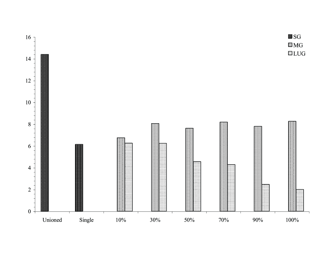
Figure 10: Total Time (hours) for $POND$ to solve all conformant and conditional problems when sampling worlds to use in heuristic computation.

There are two major points to see in Figure 10. First, the $h^{SG}_{RP}$ heuristic is much more effective when computed on $SG^{1}$ versus $SG^{U}$. This is because the $SG^{1}$ is less optimistic. It builds a planning graph for a real world state, as opposed to the union of literals in all possible world states, as in $SG^{U}$. Respecting state boundaries and considering only a single state is better than ignoring state boundaries to naively consider all possible states. However, as we have seen with the $MG$ and $LUG$ heuristics, respecting state boundaries and considering several states can be much better, bringing us to the second point.

We see very different performance when using more possible worlds to build multiple graphs compared to the $LUG$. We are better off using fewer worlds if we have to build multiple graphs because they can become very costly as the number of worlds increases. In contrast, performance improves with more possible worlds when we use the $LUG$. Using more possible worlds to compute heuristics is a good idea, but it takes a more efficient substrate to exploit them.

6.5 Accuracy

The heuristics that account for overlap in the possible worlds should be more accurate than the heuristics that make an assumption of full positive interaction or full independence. To check our intuitions, we compare the heuristic estimates for the distance between the initial belief state and the goal belief state for all the heuristics used in conformant problems solved by $POND$. Figure 11 shows the ratio of the heuristic estimate for $h(BS_{I})$ to the optimal serial plan length $h^{*}(BS_{I})$ in several problems. The points below the line (where the ratio is one) are under-estimates, and those above are over-estimates. Some of the problem instances are not shown because no optimal plan length is known.

We note that in all the domains the $h^{LUG}_{RP}$ and $h^{MG}_{RPU}$ heuristics are very close to $h^{*}$, confirming our intuitions. Interestingly, $h^{MG}_{s-RP}$ and $h^{MG}_{m-RP}$ are both close to $h^{*}$ in Rovers and Logistics; whereas the former is close in the BT and BTC problems, and the latter is close in CubeCenter and Ring. As expected, assuming independence (using summation) tends to over-estimate, and assuming positive interaction (using maximization) tends to under-estimate. The $h^{SG}_{RP}$ heuristic tends to under-estimate, and in some cases (CubeCenter and Ring) gives a value of zero (because there is an initial state that satisfies the goal). The $h_{card}$ heuristic is only accurate in BT and BTC, under-estimates in Rovers and Logistics, and over-estimates in Cube Center and Ring.

The accuracy of heuristics is in some cases disconnected from their run time performance. For instance $h_{card}$ highly overestimates in Ring and Cube Center, but does well because the domains exhibit special structure and the heuristic is fast to compute. On the other hand, $h^{LUG}_{RP}$ and $h^{MG}_{RPU}$ are very accurate in many domains, but suffer in Ring and Cube Center because they can be costly to compute.

Figure 11: Ratio of heuristic estimates for distance between $BS_{I}$ and $BS_{G}$ to optimal plan length. Rv = Rovers, L = Logistics, B = BT, BC = BTC, C = Cube Center, R = Ring.

6.6 Inter-Heuristic Conclusions

Our findings fall into two main categories: one, what are effective estimates for belief state distances in terms of state to state distances, and two, how we can exploit planning graphs to support the computation of these distance measures.

In comparing ways to aggregate state distance measures to compute belief state distances, we found that measuring no interaction as in single graph heuristics tends to poorly guide planners, measuring independence and positive interaction of worlds works well in specific domains, and measuring overlap (i.e. a combination of positive interaction and independence) tends to work well in a large variety of instances. By studying the accuracy of our heuristics we found that in some cases the most accurate were not the most effective. We did however find that the most accurate did best over the most cases.

Comparing graph structures that provide the basis for belief state distance measures, we found that the heuristics extracted from the single graph fail to systematically account for the independence or positive interaction among different possible worlds. Despite this lack in the distance measure, single graphs can still identify some structure in domains like Rovers and Logistics. To more accurately reflect belief state distances, multiple graphs reason about reachability for each world independently. This accuracy comes at the cost of computing a lot of redundant $MG$ structure and is limiting in instances with large belief states. We can reduce the cost of the $MG$ structure by sampling worlds used in its construction. However planners are able to exhibit better scalability by considering more worlds through optimizing the representation of the redundant structure as in the $LUG$. The improvement in scalability is attributed to lowering the cost of heuristic computation, but retaining measures of multiple state distances. The $LUG$ makes a trade-off of using an exponential time algorithm for evaluation of labels instead of building an exponential number of planning graphs. This trade-off is justified by our experiments.

7 Empirical Evaluation: Inter-Planner Comparison

We first compare CAltAlt and $POND$ with several planners on our conformant domains, then compare $POND$ with the conditional planners on the conditional domains. Our purpose in this section is to identify the advantages of our techniques over the state of the art planners. We end the section with a discussion of general conclusions drawn from the evaluation.

Planner	Search Space	Search Direction	Conditional	Heuristic	Implementation
CAltAlt	Belief Space	Backward		Planning Graph	C
$POND$	Belief Space	Forward	$\surd$	Planning Graph	C
MBP	Belief Space	Forward/Backward	$\surd$	Cardinality	C
KACMBP	Belief Space	Forward		Cardinality	C
CGP	Planning Graph	Backward		Planning Graph	Lisp
SGP	Planning Graph	Backward	$\surd$	Planning Graph	Lisp
GPT	Belief Space	Forward	$\surd$	State Space Plans	C
YKA	Belief Space	Backward	$\surd$	Cardinality	C
CFF	Belief Space	Forward		Planning Graph	C

Table 7: Comparison of planner features.

7.1 Conformant Planning

Although this work is aimed at giving a general comparison of heuristics for belief space planning, we also present a comparison of the best heuristics within CAltAlt and $POND$ to some of the other leading approaches to conformant planning. Table 7 lists several features of the evaluated planners, such as their search space, their search direction, whether they are conditional, the type of heuristics, and the implementation language. Note, since each approach uses a different planning representation (BDDs, GraphPlan, etc.), not all of which even use heuristics, it is hard to get a standardized comparison of heuristic effectiveness. Furthermore, not all of the planners use PDDL-like input syntax; MBP, and KACMBP use AR encodings which may give them an advantage in reducing the number of literals and actions. We gave the MBP planners the same grounded and filtered action descriptions that we used in CAltAlt and $POND$. We also tried, but do not report results, giving the MBP planners the full set of ground actions without filtering irrelevant actions. It appears that the MBP planners do not use any sort of action pre-processing because performance was much worse with the full grounded set of actions. Nevertheless, Table 8 compares MBP, KACMBP, GPT, CGP, YKA, and CFF with $h^{LUG(DyX-SX)}_{RP}$ in CAltAlt and $h^{LUG}_{RP}$ in $POND$ with respect to run time and plan length.

Problem	CAltAlt	POND	MBP	KACMBP	GPT	CGP	YKA	CFF
	$h^{LUG(DyX-SX)}_{RPU}$	$h^{LUG}_{RP}$
Rovers 1	16070/5	590/5	66/5	9293/5	3139/5	70/5	1220/7	70/5
2	10457/8	680/9	141/8	9289/15	4365/8	180/8	2050/10	30/8
3	10828/10	850/11	484/10	9293/16	5842/10	460/10	1740/12	10/10
4	15279/13	1130/16	3252/13	9371/18	7393/13	1860/13	2010/16	10/13
5	64870/29	2050/25	OoM	39773/40	399525/20	OoM	7490/27	18/22
6	221051/25	8370/25	727/32	TO	TO	-	24370/26	21/23
Logistics 1	907/9	560/9	37/9	127/12	916/9	60/6	250/13	10/9
2	2862/15	910/15	486/24	451/19	1297/15	290/6	670/19	12/15
3	10810/15	1130/14	408/14	1578/18	1711/11	400/8	20280/21	14/12
4	24862/19	3180/22	2881/27	8865/22	9828/18	1170/8	17530/27	12/18
5	54726/34	6010/29	OoM	226986/42	543865/28	TO	141910/40	25/28
BT 2	16/2	460/2	6/2	10/2	487/2	20/1	0/2	0/2
10	71/10	520/10	119/10	16/10	627/10	520/1	0/10	30/10
20	552/20	1230/20	80/20	84/20	472174/20	3200/1	20/20	4400/20
30	2415/30	4080/30	170/30	244/30	TO	10330/1	80/30	4500/30
40	7543/40	11680/40	160/40	533/40	-	24630/1	160/40	26120/40
50	17573/50	28420/50	300/50	1090/50	-	49329/1	250/50	84730/50
60	35983/60	59420/60	480/60	2123/60	-	87970/1	420/60	233410/60
70	67690/70	113110/70	730/70	3529/70	-	145270/1	620/70	522120/70
80	157655/80	202550/80	1080/80	1090/80	-	TO	3310/80	979400/80
BTC 2	16/3	460/3	8/3	18/3	465/3	0/3	10/3	10/3
10	89/19	540/19	504/19	45/19	715/19	39370/19	30/19	57/19
20	651/39	1460/39	98/39	211/39	-	-	240/39	2039/39
30	2721/59	4820/59	268/59	635/59	-	-	1210/59	23629/59
40	8009/79	14250/79	615/79	1498/79	-	-	3410/79	116156/79
50	19074/99	34220/99	1287/99	10821/99	-	-	8060/50	334879/99
60	38393/119	71650/119	2223/119	5506/119	-	-	15370/119	TO
70	65448/139	134880/139	3625/139	2640/139	-	-	27400/139	-
CubeCenter 3	TO	70/9	10/9	20/9	40/9	28990/3	0/9	20/15
5	-	1780/18	16/18	20/18	363/18	TO	0/19	28540/45
7	-	27900/29	35/27	70/27	4782/27	-	20/34	TO
9	-	177790/36	64/36	120/36	42258/36	-	80/69	-
11	-	609540/47	130/45	230/45	26549/45	-	190/68	-
Ring 2	TO	30/6	0/5	0/5	31/5	TO	0/5	360/12
3	-	70/8	0/8	40/8	35/8	-	0/8	TO
4	-	250/13	10/11	30/11	60/11	-	20/11	-
5	-	970/17	20/14	50/14	635/14	-	80/14	-
6	-	4080/22	30/17	120/18	51678/17	-	110/17	-
7	-	75020/30	80/20	230/21	TO	-	300/20	-
8	-	388300/29	160/23	600/24	-	-	480/23	-

Table 8: Results for CAltAlt using $h^{LUG(DyX-SX)}_{RP}$, $POND$ using $h^{LUG}_{RP}$, MBP, KACMBP, GPT, CGP, YKA, and CFF for conformant Rovers, Logistics, BT, BTC, Cube Center, and Ring. The data is Total Time / # Plan Steps, “TO” indicates a time out (20 minutes), “OoM” indicates out of memory (1GB), and “-” indicates no attempt.

MBP: The MBP planner uses a cardinality heuristic that in many cases overestimates plan distances (as per our implementation with $h_{card}$). MBP uses regression search for conformant plans, but progression search for conditional plans. It is interesting to note that in the more difficult problem instances in the Rovers and Logistics domains MBP and KACMBP tend to generate much longer plans than the other planners. MBP does outperform $POND$ in some cases but does not find solutions in certain instances (like Rovers 5), most likely because of its heuristic. We note that KACMBP and MBP are quite fast on the Cube Center and Ring domains, but have more trouble on domains like Rovers and Logistics. This illustrates how a heuristic modeling knowledge as opposed to reachability can do well in domains where the challenge is uncertainty not reachability.

Optimal Planners: The optimal approaches (CGP and GPT) tend not to scale as well, despite their good solutions. CGP has trouble constructing its planning graphs as the parallel conformant plan depth increases. CGP spends quite a bit of time computing mutexes, which increases the planning cost as plan lengths increase. CGP does much better on shallow and parallel domains like BT, where it can find one step plans that dunk every package in parallel.

GPT performs progression search that is guided by a heuristic that measures the cost of fully observable plans in state space. GPT finds optimal serial plans but is not as effective when the size of the search space increases. GPT fails to scale with the search space because it becomes difficult to even compute its heuristic (due to a larger state space as well).

YKA: YKA, like CAltAlt  is a regression planner, but the search engine is very different and YKA uses a cardinality heuristic. YKA performs well on all the domains because of its search engine based on BDDs. We notice a difference in progression and regression by comparing $POND$ to YKA, similar to trends found in the comparison between $POND$ and CAltAlt. Additionally, it seems YKA has a stronger regression search engine than CAltAlt. $POND$ is able to do better than YKA in the Rovers and Logistics domains, but it is unclear whether that it is because of the search direction or heuristics.

CFF: Conformant FF, a progression planner using a relaxed plan similar to the $LUG$ relaxed plan, does very well in the Rovers and Logistics domains because it uses the highly optimized FF search engine as well as a cheap to compute relaxed plan heuristic. However, CFF does not do as well in the BT, BTC, Cube Center, and Ring problems because there are not as many literals that will be entailed by a belief state. CFF relies on implicitly representing belief states in terms of the literals that are entailed by the belief state, the initial belief state, and the action history. When there are very few literals that can be entailed by the belief state, reasoning about the belief state requires inference about the action history. Another possible reason CFF suffers is our encodings. The Cube Center and Ring domains are naturally expressed with multi-valued state features, and in our transformation to binary state features we describe the values that must hold but also the values that must not hold. This is difficult for CFF because the conditional effect antecedents contain several literals and its heuristic is restricted to considering only one such literal. It may be that CFF is choosing the wrong literal or simply not enough literals to get effective heuristics. However in BT and BTC where we used only one literal in effect antecedents CFF still performs poorly.

Problem	POND	MBP	GPT	SGP	YKA
	$h^{LUG}_{RP}$
Rovers 1	580/5	3312/11	3148/5	70/5	3210/5
2	730/8	4713/75	5334/7	760/7	6400/7
3	810/8	5500/119	7434/8	TO	7490/8
4	910/10	5674/146	11430/10	-	11210/10
5	7100/19	16301/76	TO	-	TO
6	13560/22	OoM	-	-	-
Logistics 1	570/7	41/16	1023/7	5490/6	1390/8
2	1250/12	22660/177	5348/12	TO	TO
3	1210/9	2120/45	2010/8	-	TO
4	4160/15	OoM	TO	-	-
5	20170/22	-	-	-	-
BT 2	460/2	0/2	510/2	0/1	0/2
10	550/10	240/10	155314/10	70/1	20/10
20	1610/20	OoM	OoM	950/1	60/20
30	5970/30	-	-	4470/1	200/30
40	17620/40	-	-	13420/1	400/40
50	43020/50	-	-	32160/1	810/50
60	91990/60	-	-	90407/1	1350/60
70	170510/70	-	-	120010/1	2210/70
80	309940/80	-	-	TO	3290/80
BTC 2	470/2	20/2	529/2	10/2	0/4
10	590/10	280/10	213277/10	TO	210/12
20	1960/20	OoM	TO	-	2540/22
30	6910/30	-	-	-	13880/32
40	19830/40	-	-	-	46160/42
50	49080/50	-	-	-	109620/52
60	103480/60	-	-	-	221460/62
70	202040/70	-	-	-	41374/72

Table 9: Results for $POND$ using $h^{LUG}_{RP}$, MBP, GPT, SGP, and YKA for conditional Rovers, Logistics, BT, and BTC. The data is Total Time / # Maximum possible steps in a execution, “TO” indicates a time out (20 minutes), “OoM” indicates out of memory (1GB), and “-” indicates no attempt.

7.2 Conditional Planning

Table 9 shows the results for testing the conditional versions of the domains on $POND$, MBP, GPT, SGP, and YKA.

MBP: The $POND$ planner is very similar to MBP in that it uses progression search. $POND$ uses an AO* search, whereas the MBP binary we used uses a depth first And-Or search. The depth first search used by MBP contributes to highly sub-optimal maximum length branches (as much as an order of magnitude longer than $POND$). For instance, the plans generated by MBP for the Rovers domain have the rover navigating back and forth between locations several times before doing anything useful; this is not a situation beneficial for actual mission use. MBP tends to not scale as well as $POND$ in all of the domains we tested. A possible reason for the performance of MBP is that the Logistics and Rovers domains have sensory actions with execution preconditions, which prevent branching early and finding deterministic plan segments for each branch. We experimented with MBP using sensory actions without execution preconditions and it was able to scale somewhat better, but plan quality was much longer.

Optimal Planners: GPT and SGP generate better solutions but very slowly. GPT does better on the Rovers and Logistics problems because they exhibit some positive interaction in the plans, but SGP does well on BT because its planning graph search is well suited for shallow, yet broad (highly parallel) problems.

YKA: We see that YKA fares similar to GPT in Rovers and Logistics, but has trouble scaling for other reasons. We think that YKA may be having trouble in regression because of sensory actions since it was able to scale reasonably well in the conformant version of the domains. Despite this, YKA proves to do very well in the BT and BTC problems.

7.3 Empirical Evaluation Conclusions

In our internal comparisons of heuristics within CAltAlt and $POND$, as well as external comparisons with several state of the art conformant and conditional planners we have learned many interesting lessons about heuristics for planning in belief space.

• Distance based heuristics for belief space search help control conformant and conditional plan length because, as opposed to cardinality, the heuristics model desirable plan quality metrics.

• Planning graph heuristics for belief space search scale better than planning graph search and admissible heuristic search techniques.

• Of the planning graph heuristics presented, relaxed plans that take into account the overlap of individual plans between states of the source and destination belief states are the most accurate and tend to perform well across many domains.

• The LUG is an effective planning graph for both regression and progression search heuristics.

• In regression search, planning graphs that maintain only same-world mutexes provide the best trade-off between graph construction cost and heuristic informedness.

• Sampling possible worlds to construct planning graphs does reduce computational cost, but considering more worlds by exploiting planning graph structure common to possible worlds (as in the $LUG$), can be more efficient and informed.

• The LUG heuristics help our conditional planner, $POND$, to scale up in conditional domains, despite the fact that the heuristic computation does not model observation actions.

8 Related Work & Discussion

We discuss connections with several related works that involve heuristics and/or conditional planning in the first half of this section. In the second part of the section we discuss how we can extend our work to directly handle non-deterministic outcomes of actions in heuristic computation.

8.1 Related Work

Much interest in conformant and conditional planning can be traced to CGP (?), a conformant version of GraphPlan (?), and SGP (?), the analogous conditional version of GraphPlan. Here the graph search is conducted on several planning graphs, each constructed from one of the possible initial states. More recent work on C-plan (?) and Frag-Plan (?) generalize the CGP approach by ordering the searches in the different worlds such that the plan for the hardest to satisfy world is found first, and is then extended to the other worlds. Although ${\cal C}{\sl AltAlt}$ and $POND$ utilize planning graphs similar to CGP and Frag-plan it only uses them to compute reachability estimates. The search itself is conducted in the space of belief states.

Another strand of work models conformant and conditional planning as a search in the space of belief states. This started with ? (?), who concentrated on formulating a set of admissible pruning conditions for controlling search. There were no heuristics for choosing among unpruned nodes. GPT (?) extended this idea to consider a simple form of reachability heuristic. Specifically, in computing the estimated cost of a belief state, GPT assumes that the initial state is fully observable. The cost estimate itself is done in terms of reachability (with dynamic programming rather than planning graphs). GPT’s reachability heuristic is similar to our $h_{m-RP}^{MG}$ heuristic because they both estimate the cost of the farthest (maximum distance) state by looking at a deterministic relaxation of the problem. In comparison to GPT, ${\cal C}{\sl AltAlt}$ and $POND$ can be seen as using heuristics that do a better job of considering the cost of the belief state across the various possible worlds.

Another family of planners that search in belief states is the MBP-family of planners—MBP (?), and KACMBP (?). In contrast to ${\cal C}{\sl AltAlt}$ but similar to $POND$, the MBP-family of planners all represent belief states in terms of binary decision diagrams. Action application is modeled as modifications to the BDDs. MBP supports both progression and regression in the space of belief states, while KACMBP is a pure progression planner. Before computing heuristic estimates, KACMBP pro-actively reduces the uncertainty in the belief state by preferring uncertainty reducing actions. The motivation for this approach is that applying cardinality heuristics to belief states containing multiple states may not give accurate enough direction to the search. While reducing the uncertainty seems to be an effective idea, we note that (a) not all domains may contain actions that reduce belief state uncertainty and (b) the need for uncertainty reduction may be reduced when we have heuristics that effectively reason about the multiple worlds (viz., our multiple planning graph heuristics). Nevertheless, it could be very fruitful to integrate knowledge goal ideas of KACMBP and the reachability heuristics of ${\cal C}{\sl AltAlt}$ and $POND$ to handle domains that contain both high uncertainty and costly goals.

In contrast to these domain-independent approaches that only require models of the domain physics, PKSPlan (?) is a forward-chaining knowledge-based planner that requires richer domain knowledge. The planner makes use of several knowledge bases, as opposed to a single knowledge base taking the form of a belief state. The knowledge bases separate binary and multi-valued variables, and planning and execution time knowledge.

YKA (?) is a regression conditional planner using BDDs that uses a cardinality heuristic. Recently Rintanen has also developed related reachability heuristics that consider distances for groups of states, which do not rely on planning graphs (?).

More recently, there has been closely related work on heuristics for constructing conformant plans within the CFF planner (?). The planner represents belief states implicitly through a set of known facts, the action history (leading to the belief state), and the initial belief state. CFF builds a planning graph forward from the set of known literals to the goal literals and backwards to the initial belief state. In the planning graph, conditional effects are restricted to single literals in their antecedent to enable tractable 2-cnf reasoning. From this planning graph, CFF extracts a relaxed plan that represents supporting the goal belief state from all states in the initial belief state. The biggest differences between the $LUG$ and the CFF technique are that the $LUG$ reasons only forward from the source belief state (assuming an explicit, albeit symbolic, belief state), and the $LUG$ does not restrict the number of literals in antecedents. As a result, the $LUG$ does not lose the causal information nor perform backward reasoning to the initial belief state.

Our handling of uncertainty through labels and label propagation is reminiscent of and related to de Kleer’s assumption based truth maintenance system (ATMS) (?). Where an ATMS uses labels to identify the assumptions (contexts) where a particular statement holds, a traditional truth maintenance system requires extensive backtracking and consistency enforcement to identify other contexts. Similarly, where we can reason about multiple possible worlds (contexts) with the LUG simultaneously, the MG approach requires, not backtracking, but reproduction of planning graphs for other possible worlds.

Finally, ${\cal C}{\sl AltAlt}$ and $POND$ are also related to, and an adaptation of the work on reachability heuristics for classical planning, including $AltAlt$ (?), FF (?) and HSP-r (?). ${\cal C}{\sl AltAlt}$ is the conformant extension to $AltAlt$ that uses regression search (similar to HSP-r) guided by planning graph heuristics. $POND$ is similar to FF in that it uses progression search with planning graph heuristics.

8.2 Extension to Non-Deterministic Actions

While the scope of our presentation and evaluation is restricted to planning with initial state uncertainty and deterministic actions, some of the planning graph techniques can be extended to include non-deterministic actions of the type described by ? (?). Non-deterministic actions have effects that are described in terms of a set of outcomes. For simplicity, we consider Rintanen’s conditionality normal form, where actions have a set of conditional effects (as before) and each consequent is a mutually-exclusive set of conjunctions (outcomes) – one outcome of the effect will result randomly. We outline the generalization of our single, multiple, and labelled planning graphs to reason with non-deterministic actions.

Single Planning Graphs: Single planning graphs, that are built from approximate belief states or a sampled state, do not lend themselves to a straight-forward extension. A single graph ignores uncertainty in a belief state by unioning its literals or sampling a state to form the initial planning graph layer. Continuing with the single graph assumptions about uncertainty, it makes sense to treat non-deterministic actions as deterministic. Similar to how we approximate a belief state as a set of literals to form the initial literal layer or sample a state, we can assume that a non-deterministic effect adds all literals appearing in the effect or samples an outcome as if the action were deterministic (i.e. gives a set of literals). Single graph relaxed plan heuristics thus remain unchanged.

Multiple Planning Graphs: Multiple planning graphs are very much like Conformant GraphPlan (?). We can generalize splitting the non-determinism in the current belief state into multiple initial literal layers to splitting the outcomes of non-deterministic effects into multiple literal layers. The idea is to root a set of new planning graphs at each level, where each has an initial literal layer containing literals supported by an interpretation of the previous effect layer. By interpretations of the effect layer we mean every possible set of joint effect outcomes. A set of effect outcomes is possible if no two outcomes are outcomes of the same effect. Relaxed plan extraction still involves finding a relaxed plan in each planning graph. However, since each planning graph is split many times (in a tree-like structure) a relaxed plan is extracted from each “path of the tree”.

We note that this technique is not likely to scale because of the exponential growth in redundant planning graph structure over time. Further, in our experiments CGP has enough trouble with initial state uncertainty. We expect that we should be able to do much better with the $LUG$.

Labelled Uncertainty Graph: With multiple planning graphs we are forced to capture non–determinism through splitting the planning graphs not only in the initial literal layer, but also each literal layer that follows at least one non-deterministic effect. We saw in the $LUG$ that labels can capture the non-determinism that drove us to split the initial literal layer in multiple graphs. As such, these labels took on a syntactic form that describes subsets of the states in our source belief state. In order to generalize labels to capture non-determinism resulting from uncertain effects, we need to extend their syntactic form. Our objective is to have a label represent which sources of uncertainty (arising from the source belief state or effects) causally support the labelled item. We also introduce a graph layer ${\cal O}_{k}$ to represent outcomes and how they connect effects and literals.

It might seem natural to describe the labels for outcomes in terms of their affected literals, but this can lead to trouble. The problem is that the literals in effect outcomes are describing states at a different time than the literals in the projected belief state. Further, an outcome that appears in two levels of the graph is describing a random event at different times. Using state literals to describe all labels will lead to confusion as to which random events (state uncertainty and effect outcomes at distinct steps) causally support a labelled item. A pathological example is when we have an effect whose set of outcomes matches one-to-one with the states in the source belief state. In such a case, by using labels defined in terms of state literals we cannot distinguish which random event (the state uncertainty or the effect uncertainty) is described by the label.

We have two choices for describing effect outcomes in labels. In both choices we introduce a new set of label variables to describe how a literal layer is split. These new variables will be used to describe effect outcomes in labels and will not be confused with variables describing initial state uncertainty. In the first case, these variables will have a one-to-one matching with our original set of literals, but can be thought of as time-stamped literals. The number of variables we add to the label function is on the order of 2$F$ per level (the number of fluent literals – assuming boolean fluents). The second option is to describe outcomes in labels with a new set of fluents, where each interpretation over the fluents is matched to a particular outcome. In this case, we add on the order of log $|{\cal O}_{k}|$ variables, where ${\cal O}_{k}$ is the $k^{th}$ outcome layer. It would actually be lower if many of the outcomes were from deterministic effects because there is no need to describe them in labels. The former approach is likely to introduce fewer variables when there are a lot of non-deterministic effects and they affect quite a few of the same literals. The latter will introduce fewer variables when there are relatively few non-deterministic effects whose outcomes are fairly independent.

With the generalized labelling, we can still say that an item is reachable from the source belief state when its label is entailed by the source belief state. This is because even though we are adding variables to labels, we are implicitly adding the fluents to the source belief state. For example, say we add a fluent $v$ to describe two outcomes of an effect. One outcome is labelled $v$, the other $\neg v$. We can express the source belief state $BS_{P}$ that is projected by the $LUG$ with the new fluent as $BS_{P}\wedge(v\vee\neg v)=BS_{P}$. An item labelled as $BS_{P}\wedge v$ will not be entailed by the projected belief state (i.e. is unreachable) because only one outcome causally supports it. If both outcomes support the item, then it will be reachable.

Given our notion of reachability, we can determine the level from which to extract a relaxed plan. The relaxed plan procedure does not change much in terms of its semantics other than having the extra graph layer for outcomes. We still have to ensure that literals are causally supported in all worlds they are labelled with in a relaxed plan, whether or not the worlds are from the initial state uncertainty or supporting non-deterministic effects.

9 Conclusion

With the intent of establishing a basis for belief state distance estimates, we have:

• Discussed how heuristic measures can aggregate state distance measures to capture positive interaction, negative interaction, independence, and overlap.

• Shown how to compute such heuristic measures on planning graphs and provided empirical comparisons of these measures.

• Found that exploiting planning graph structure to reduce the cost of considering more possible states of a belief state is preferable to sampling a subset of the states for the heuristics.

• Shown that a labelled uncertainty graph can capture the same support information as multiple graphs, and reduces the cost of heuristic computation.

• Shown that the labelled uncertainty graph is very useful for conformant planning and, without considering observational actions and knowledge, can perform well in conditional planning.

Our intent in this work was to provide a formal basis for measuring the distance between belief states in terms of underlying state distances. We investigated several ways to aggregate the state distances to reflect various assumptions about the interaction of state to state trajectories. The best of these measures turned out to measure both positive interaction and independence, what we call overlap. We saw that planners using this notion of overlap tend to do well across a large variety of domains and tend to have more accurate heuristics.

We’ve also shown that planning with a Labelled Uncertainty planning Graph $LUG$, a condensed version of the multiple graphs is useful for encoding conformant reachability information. Our main innovation is the idea of “labels” – labels are attached to all literals, actions, effect relations, and mutexes to indicate the set of worlds in which those respective elements hold. Our experimental results show that the $LUG$ can outperform the multiple graph approach. In comparison to other approaches, we’ve also been able to demonstrate the utility of structured reachability heuristics in controlling plan length and boosting scalability for both conformant and conditional planning.

We intend to investigate three additions to this work. The first, is to incorporate sensing and knowledge into the heuristics. We already have some promising results without using these features in the planning graphs, but hope that they will help the approaches scale even better on conditional problems. The second addition will be to consider heuristics for stochastic planning problems. The major challenges here are to associate probabilities with labels to indicate the likelihood of each possible world and integrate reasoning about probabilistic action effects.

Lastly, we have recently extended the $LUG$ within the framework of state agnostic planning graphs (?), and hope to improve the technique. A state agnostic planning graph is essentially a multiple source planning graph, where by analogy a conventional planning graph has a single source. Planning graphs are already multiple destination, so in our generalization the state agnostic planning graph allows us to compute the distance measure between any pair of states or belief states. The $LUG$ seeks to avoid redundancy across the multiple planning graphs built for states in the same belief state. We extended this notion to avoid redundancy in planning graphs built for every belief state. We have shown that the state agnostic $LUG$ ($SLUG$) which is built once per search episode (as opposed to a $LUG$ at each node) can reduce heuristic computation cost without sacrificing informedness.

Acknowledgments

We would like to thank Minh B. Do, Romeo Sanchez, Terry Zimmermam, Satish Kumar Thittamaranahalli, and Will Cushing for helpful discussions and feedback, Jussi Rintanen for help with the YKA planner, and Piergiorgio Bertoli for help with the MBP planner. This work was supported in part by NASA grants NCC2-1225 and NAG2-1461, the NSF grant IIS-0308139, the 2003 NASA RIACS SSRP, the ARCS Foundation, and an IBM faculty award.

A Additional Heuristics

For completeness, we present some additional heuristics adapted from classical planning to reason about belief state distances in each type of planning graph. Many of these heuristics appeared in our previous work (?). We show how to compute the max, sum, and level heuristics on the single graph $SG$, multiple graphs $MG$, and the labelled uncertainty graph $LUG$. While these heuristics tend to be less effective than the relaxed plan heuristics, we provide them as reference. As with Section 4, we describe the heuristics in terms of regression search.

A.1 Single Planning Graph Heuristics ($SG$)

Like, the relaxed plan for the single unmodified planning graph, we cannot aggregate state distances because all notion of separate states is lost in forming the initial literal layer, thus we only compute heuristics that do not aggregate state distances.

No State Aggregation:

• Max In classical planning, the maximum cost literal is used to get a max heuristic, but we use formulas to describe our belief states, so we take the maximum cost clause as the cost of the belief state to find the max heuristic $h^{SG}_{max}$. The maximum cost clause of the belief state, with respect to a single planning graph, is:

  $$h^{SG}_{max}(BS_{i})=\max\limits_{C\in{\kappa(BS_{i})}}cost(C)$$

  where the cost of a clause is:

  $$cost(C)=\min\limits_{l\in{C}}\min\limits_{k:l\in{\cal L}_{k}}k$$

  Here we find the cheapest literal as the cost of each clause to find the maximum cost clause. This is an underestimate of the closest state to our current belief state.

• Sum Like the classical planning sum heuristic, we can take the sum $h^{SG}_{sum}$ of the costs of the clauses in our belief state to estimate our belief state distance

  $$h^{SG}_{sum}(BS_{i})=\sum\limits_{C\in{\kappa(BS_{i})}}cost(C)$$

  This heuristic takes the summation of costs of literals in the closest estimated state in the belief state, and is inadmissible because there may be a single action that will support every clause, and we could count it once for each clause.

• Level When we have mutexes on the planning graph, we can compute a level heuristic $h^{SG}_{level}$ (without mutexes the level heuristic is equivalent to the max heuristic). The level heuristic maintains the admissibility of the max heuristic but improves the lower bound by considering what level of the planning graph all literals in a constituent are non-pairwise mutex. The level heuristic is computed by taking the minimum among the $\hat{S}\in\hat{\xi}(BS_{i})$, of the first level ($lev({S})$) in the planning graph where literals of $\hat{S}$ are present with none of them marked pairwise mutex. Formally:

  $$h^{SG}_{level}(BS_{i})=\min\limits_{\hat{S}\in\hat{\xi}(BS_{i})}lev(\hat{S})$$

A.2 Multiple Planning Graph Heuristics ($MG$)

Similar to the various relaxed plan heuristics for the multiple graphs, we can compute a max, sum, or level heuristic on each of the multiple planning graphs and aggregate them with a maximum or summation to respectively measure positive interaction or independence. The reason we cannot aggregate the individual graph heuristics to measure overlap is that they are numbers, not sets of actions. Measuring overlap involves taking the union of heuristics from each graph and the union of numbers is not meaningful like the union of action sets from relaxed plans. Like before, there is no reason to use multiple graphs if there is no state distance aggregation.

Positive Interaction Aggregation:

• Max The max heuristic $h^{MG}_{m-max}$ is computed with multiple planning graphs to measure positive interaction in the $h^{MG}_{m-max}$ heuristic. This heuristic computes the maximum cost clause in $\kappa(BS_{i})$ for each graph $\gamma\in\Gamma$, similar to how $h^{SG}_{m-max}(BS_{i})$ is computed, and takes the maximum. Formally:

  $$h^{MG}_{m-max}(BS_{i})=\max\limits_{\gamma\in{\Gamma}}\left(h^{\gamma}_{max}(BS_{i})\right)$$

  The $h^{MG}_{m-max}$ heuristic considers the minimum cost, relevant literals of a belief state (those that are reachable given a possible world for each graph $\gamma$) to get state measures. The maximum is taken because the estimate accounts for the worst (i.e., the plan needed in the most difficult world to achieve the subgoals).

• Sum The sum heuristic that measures positive interaction for multiple planning graphs is $h^{MG}_{m-sum}$. It computes the summation of the cost of the clauses in $\kappa(BS_{i})$ for each graph $\gamma\in\Gamma$ and takes the maximum. Formally:

  $$h^{MG}_{m-sum}(BS_{i})=\max\limits_{\gamma\in{\Gamma}}\left(h^{\gamma}_{sum}(BS_{i})\right)$$

  The heuristic considers the minimum cost, relevant literals of a belief state (those that are reachable given the possible worlds represented for each graph $\gamma$) to get state measures. As with $h^{MG}_{m-max}$, the maximum is taken to estimate for the most costly world.

• Level Similar to $h^{MG}_{m-max}$ and $h^{MG}_{m-sum}$, the $h^{MG}_{m-level}$ heuristic is found by first finding $h^{\gamma}_{level}$ for each graph $\gamma\in\Gamma$ to get a state distance measure, and then taking the maximum across the graphs. $h^{\gamma}_{level}(BS_{i})$ is computed by taking the minimum among the $\hat{S}\in\hat{\xi}(BS_{i})$, of the first level $lev^{\gamma}(\hat{S})$ in the planning graph $\gamma$ where literals of $\hat{S}$ are present with none of them marked mutex. Formally:

  $$h^{\gamma}_{level}(BS_{i})=\min\limits_{\hat{S}\in\hat{\xi}(BS_{i})}lev^{\gamma}(\hat{S})$$

  and

  $$h^{MG}_{m-level}(BS_{i})=\max\limits_{\gamma\in{\Gamma}}(h^{\gamma}_{level}(BS_{i}))$$

  Note that this heuristic is admissible. By the same reasoning as in classical planning, the first level where all the subgoals are present and non-mutex is an underestimate of the true cost of a state. This holds for each of the graphs. Taking the maximum accounts for the most difficult world in which to achieve a constituent of $BS_{i}$ and is thus a provable underestimate of $h^{*}$. GPT’s max heuristic (?) is similar to $h^{MG}_{m-level}$, but is computed with dynamic programming in state space rather than planning graphs.

Independence Aggregation: All heuristics mentioned for Positive Interaction Aggregation can be augmented to take the summation of costs found on the individual planning graphs rather than the maximum. We denote them as: $h^{MG}_{s-max}$, $h^{MG}_{s-sum}$, and $h^{MG}_{s-level}$. None of these heuristics are admissible because the same action may be used in all worlds, but we count its cost for every world by using summation.

A.3 Labelled Uncertainty Graph ($LUG$)

The max, sum, and level heuristics for the $LUG$ are similar to the analogous multiple graph heuristics. The main difference with these heuristics for the $LUG$ is that it is much easier to compute positive interaction measures than independence measures. The reason positive interaction is easier to compute is that we find the cost of a clause for all states in our belief state at once, rather than on each of multiple planning graphs. Like before, we do not consider heuristics that do not aggregate state distances.

Positive Interaction Aggregation:

• Max The max heuristic $h^{LUG}_{m-max}$ for the $LUG$ finds the maximum clause cost across clauses of the current belief state $BS_{i}$. The cost of a clause is the first level it becomes reachable. Formally:

  $$h^{LUG}_{m-max}(BS_{i})=\max\limits_{C\in\kappa(BS_{i})}\left(\min\limits_{k:BS_{P}\models\ell_{k}^{*}(C)}k\right)$$

• Sum The sum heuristic $h^{LUG}_{m-sum}$ for the $LUG$ sums the individual levels where each clause in $\kappa(BS_{i})$ is first reachable. Formally:

  $$h^{LUG}_{m-sum}(BS_{i})=\sum\limits_{C\in\kappa(BS_{i})}\left(\min\limits_{k:BS_{P}\models\ell_{k}^{*}(C)}k\right)$$

• Level The level heuristic $h^{LUG}_{m-level}$ is the index of the first level where $BS_{i}$ is reachable. Formally:

  $$h^{LUG}_{m-level}(BS_{i})=\min\limits_{k:BS_{P}\models\ell_{k}^{*}(BS_{i})}i$$

Independence Aggregation: All heuristics mentioned for positive interaction aggregation can be augmented to take the summation of costs for each state in our belief state. This may be inefficient due to the fact that we lose the benefit of having a $LUG$ by evaluating a heuristic for each state of our $BS_{P}$, rather than all states at once as in the positive interaction aggregation. In such a case we are doing work similar to the multiple graph heuristic extraction, aside from the improved graph construction time. The positive interaction aggregation is able to implicitly calculate the maximum over all worlds for most of the heuristics, whereas for the sum heuristic we need to explicitly find a cost for each world. We denote the sum heuristics as: $h^{LUG}_{s-max}$, $h^{LUG}_{s-sum}$, and $h^{LUG}_{s-level}$.

B Cross-World Mutexes

Mutexes can develop not only in the same possible world but also between two possible worlds, as described by ? (?). Cross-world mutexes are useful to capture negative interactions in belief state distance measures (mentioned in Section 3). The representation of cross-world mutexes requires another generalization for the labelling of mutexes. Same world mutexes require keeping only one label for the mutex to signify all same possible worlds for which the mutex holds. The extended representation keeps a pair of labels, one for each element in the mutex; if $x$ in possible world $S$ is mutex with $x^{\prime}$ in possible world $S^{\prime}$, we denote the mutex as the pair ($\hat{\ell}_{k}(x)=S,\hat{\ell}_{k}(x^{\prime})=S^{\prime}$).

We can compute cross-world mutexes between several worlds of elements $x$ and $x^{\prime}$. For example, if $\ell_{k}(x)=S_{1}\vee S_{2}\vee S_{3}$ and $\ell_{k}(x^{\prime})=S_{2}\vee S_{3}$, then to check for all cross-world mutexes we need to consider mutexes for the world pairs $(S_{1},S_{2}),(S_{1},S_{3}),(S_{2},S_{2}),(S_{2},S_{3}),(S_{3},S_{2})$, and $(S_{3},S_{3})$. We can also check for mutexes in the intersection of the element labels $\ell_{k}(x)\wedge\ell_{k}(x^{\prime})=S_{2}\vee S_{3}$, meaning the only cross world pairs we check for mutexes are $(S_{2},S_{2}),(S_{2},S_{3}),(S_{3},S_{2})$, and $(S_{3},S_{3})$.

We can say that a formula $f$ is reachable from our projected belief state $BS_{P}$, when considering cross-world mutexes, if for every pair of states in $BS_{P}$, $f$ is reachable. For a pair of states $S$ and $S^{\prime}$, $f$ is reachable if $S\wedge S^{\prime}\models\ell_{k}^{*}(f)$ and for every pair of constituents $\hat{S^{\prime\prime}},\hat{S^{\prime\prime\prime}}\in\hat{f}$ such that $S\models\ell_{k}^{*}(\hat{S^{\prime\prime}})$ and $S^{\prime}\models\ell_{k}^{*}(\hat{S^{\prime\prime\prime}})$, there are no two literals in either $\hat{S^{\prime\prime}}$ or $\hat{S^{\prime\prime\prime}}$ that are same-world mutex when $S=S^{\prime}$, and there is not a mutex between literals in $\hat{S^{\prime\prime}}$ and $\hat{S^{\prime\prime\prime}}$, across the respective worlds $S$ and $S^{\prime}$ when $S\neq S^{\prime}$. There is a mutex between a pair literals $l$ and $l^{\prime}$, respectively from $\hat{S^{\prime\prime}}$ and $\hat{S^{\prime\prime\prime}}$ if there is a mutex $(\hat{\ell}_{k}(l),\hat{\ell}_{k}(l^{\prime}))$ such that $S\models\hat{\ell}_{k}(l)$ and $S^{\prime}\models\hat{\ell}_{k}(l^{\prime})$.

The computation of cross-world mutexes requires changes to some of the mutex formulas, as outlined next. The major change is to check, instead of all the single possible worlds $S$, all pairs of possible worlds $S$ and $S^{\prime}$ for mutexes.

Action Mutexes: The action mutexes can now hold for actions that are executable in different possible worlds.

• Interference Interference mutexes do not change for cross-world mutexes, except that there is a pair of labels where ($\hat{\ell}_{k}(a)=BS_{P},\hat{\ell}_{k}(a^{\prime})=BS_{P}$), instead of a single label.

• Competing Needs Competing needs change mutexes for cross-world mutexes because two actions $a$ and $a^{\prime}$, in worlds $S$ and $S^{\prime}$ respectively, could be competing. Formally, a cross-world competing needs mutex ($(\hat{\ell}_{k}(a)=S,\hat{\ell}_{k}(a^{\prime})=S^{\prime}$) exists between $a$ and $a^{\prime}$ in worlds $S$ and $S^{\prime}$ if:

  $$\exists_{l\in\rho^{e}(a),l^{\prime}\in\rho^{e}(a^{\prime})}(\hat{\ell}_{k}(l)=S,\hat{\ell}_{k}(l^{\prime})=S^{\prime})$$

Effect Mutexes: The effect mutexes can now hold for effects that occur in different possible worlds.

• Interference Effect interference mutexes do not change for cross-world mutexes, except that there is a pair of labels where ($\hat{\ell}_{k}(\varphi^{i}(a))=BS_{P},\hat{\ell}_{k}(\varphi^{j}(a^{\prime}))=BS_{P}$), instead of a single label.

• Competing Needs Effect competing needs mutexes change for cross-world mutexes because two effects $\varphi^{i}(a)$ and $\varphi^{j}(a^{\prime})$, in worlds $S$ and $S^{\prime}$ respectively, could be competing. Formally, a cross-world competing needs mutex ($\hat{\ell}_{k}(\varphi^{i}(a))=S,\hat{\ell}_{k}(\varphi^{j}(a^{\prime}))=S^{\prime}$) exists between $\varphi^{i}(a)$ and $\varphi^{j}(a^{\prime})$ in worlds $S$ and $S^{\prime}$ if:

  $$\exists_{l\in\rho^{i}(a),l^{\prime}\in\rho^{j}(a^{\prime})}(\hat{\ell}_{k}(l)=S,\hat{\ell}_{k}(l^{\prime})=S^{\prime})$$

• Induced Induced mutexes change slightly for cross-world mutexes. The worlds where one effect induces another, remains the same, but the mutex changes slightly.

  If $\varphi^{j}(a)$ in $\hat{\ell}_{k}(\varphi^{j}(a))$ is mutex with $\varphi^{h}(a^{\prime})$ in $\hat{\ell}_{k}(\varphi^{h}(a^{\prime}))$, and $\varphi^{i}(a)$ induces effect $\varphi^{j}(a)$ in the possible worlds described by $\ell_{k}(\varphi^{i}(a))\wedge\ell_{k}(\varphi^{j}(a))$, then there is an induced mutex between $\varphi^{i}(a)$ in $\hat{\ell_{k}}(\varphi^{j}(a))\wedge\ell_{k}(\varphi^{i}(a))$ and $\varphi^{h}(a^{\prime})$ in $\hat{\ell_{k}}(\varphi^{h}(a^{\prime}))$ (see Figure 12).

  

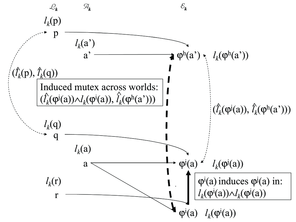
  Figure 12: Example of a cross-world induced effect mutex.

Literal Mutexes: The literal mutexes can now hold for literals that are supported in different possible worlds.

• Inconsistent Support changes for cross-world mutexes. A mutex ($\hat{\ell}_{k}(l)=S,\hat{\ell}_{k}(l^{\prime})=S^{\prime}$) holds for $l$ in $S$ and $l^{\prime}$ in $S^{\prime}$ if $\forall\varphi^{i}(a),\varphi^{j}(a^{\prime})\in{\cal E}_{k-1}$ where $l\in\varepsilon^{i}(a),l^{\prime}\in\varepsilon^{j}(a^{\prime})$, there is a mutex $\hat{\ell}_{k-1}(\varphi^{i}(a))=S,\hat{\ell}_{k-1}(\varphi^{j}(a^{\prime}))=S^{\prime})$.

References

- Bertoli and Cimatti Bertoli, P., and Cimatti, A. (2002). Improving heuristics for planning as search in belief space. In Proceedings of AIPS’02.
- Bertoli et al. Bertoli, P., Cimatti, A., and Roveri, M. (2001a). Heuristic search + symbolic model checking = efficient conformant planning. In Proceedings of IJCAI’01.
- Bertoli et al. Bertoli, P., Cimatti, A., Roveri, M., and Traverso, P. (2001b). Planning in nondeterministic domains under partial observability via symbolic model checking. In Proceedings of IJCAI’01.
- Blum and Furst Blum, A., and Furst, M. (1995). Fast planning through planning graph analysis. In Proceedings of IJCAI’95.
- Bonet and Geffner Bonet, B., and Geffner, H. (1999). Planning as heuristic search: New results. In Proceedings of ECP’99.
- Bonet and Geffner Bonet, B., and Geffner, H. (2000). Planning with incomplete information as heuristic search in belief space. In Proceedings of AIPS’00.
- Brace et al. Brace, K., Rudell, R., and Bryant, R. (1990). Efficient implementation of a bdd package. In Proceedings of the 27th ACM/IEEE design automation conference.
- Bryant Bryant, R. (1986). Graph-based algorithms for Boolean function manipulation. IEEE Transactions on Computers, C-35(8), 677–691.
- Bryce and Kambhampati Bryce, D., and Kambhampati, S. (2004). Heuristic guidance measures for conformant planning. In Proceedings of ICAPS’04.
- Castellini et al. Castellini, C., Giunchiglia, E., and Tacchella, A. (2001). Improvements to sat-based conformant planning. In Proceedings of ECP’01.
- Cimatti and Roveri Cimatti, A., and Roveri, M. (2000). Conformant planning via symbolic model checking. Journal of Artificial Intelligence Research, 13, 305–338.
- Cormen et al. Cormen, T. H., Leiserson, C. E., and Rivest, R. L. (1990). Introduction to Algorithms. McGraw-Hill.
- Cushing and Bryce Cushing, W., and Bryce, D. (2005). State agnostic planning graphs. In Proceedings of AAAI’05.
- de Kleer de Kleer, J. (1986). An Assumption-Based TMS. Artificial Intelligence, 28(2), 127–162.
- Genesereth and Nourbakhsh Genesereth, M. R., and Nourbakhsh, I. R. (1993). Time-saving tips for problem solving with incomplete information. In Proceedings of AAAI’93.
- Hansen and Zilberstein Hansen, E., and Zilberstein, S. (2001). LAO: A heuristic-search algorithm that finds solutions with loops. Artificial Intelligence, 129(1–2), 35–62.
- Hoffmann and Brafman Hoffmann, J., and Brafman, R. (2004). Conformant planning via heuristic forward search: A new approach. In Proceedings of ICAPS’04.
- Hoffmann and Nebel Hoffmann, J., and Nebel, B. (2001). The FF planning system: Fast plan generation through heuristic search. Journal of Artificial Intelligence Research, 14, 253–302.
- Kambhampati et al. Kambhampati, S., Ihrig, L., and Srivastava, B. (1996). A candidate set based analysis of subgoal interactions in conjunctive goal planning. In Proceedings of AIPS’96.
- Koehler et al. Koehler, J., Nebel, B., Hoffmann, J., and Dimopoulos, Y. (1997). Extending planning graphs to an adl subset. In Proceedings of ECP’97.
- Kurien et al. Kurien, J., Nayak, P., and Smith, D. (2002). Fragment-based conformant planning. In Proceedings of AIPS’02.
- Long and Fox Long, D., and Fox, M. (2003). The 3rd international planning competition: Results and analysis. Journal of Artificial Intelligence Research, 20, 1–59.
- Nguyen et al. Nguyen, X., Kambhampati, S., and Nigenda, R. (2002). Planning graph as the basis for deriving heuristics for plan synthesis by state space and CSP search. Artificial Intelligence, 135(1-2), 73–123.
- Nilsson Nilsson, N. (1980). Principles of Artificial Intelligence. Morgan Kaufmann.
- Pednault Pednault, E. P. D. (1988). Synthesizing plans that contain actions with context-dependent effects. Computational Intelligence, 4, 356–372.
- Petrick and Bacchus Petrick, R., and Bacchus, F. (2002). A knowledge-based approach to planning with incomplete information and sensing. In Proceedings of AIPS’02.
- Rintanen Rintanen, J. (2003a). Expressive equivalence of formalisms for planning with sensing. In Proceedings of ICAPS’03.
- Rintanen Rintanen, J. (2003b). Product representation of belief spaces in planning under partial observability. In Proceedings of IJCAI’03.
- Rintanen Rintanen, J. (2004). Distance estimates for planning in the discrete belief space. In Proceedings of AAAI’04.
- Smith and Weld Smith, D., and Weld, D. (1998). Conformant graphplan. In Proceedings of AAAI’98.
- Weld et al. Weld, D., Anderson, C., and Smith, D. (1998). Extending graphplan to handle uncertainty and sensing actions. In Proceedings of AAAI’98.