Advances in Global and Local Helioseismology: an Introductory Review

Abstract

Helioseismology studies the structure and dynamics of the Sun’s interior by observing oscillations on the surface. These studies provide information about the physical processes that control the evolution and magnetic activity of the Sun. In recent years, helioseismology has made substantial progress towards the understanding of the physics of solar oscillations and the physical processes inside the Sun, thanks to observational, theoretical and modeling efforts. In addition to the global seismology of the Sun based on measurements of global oscillation modes, a new field of local helioseismology, which studies oscillation travel times and local frequency shifts, has been developed. It is capable of providing 3D images of the subsurface structures and flows. The basic principles, recent advances and perspectives of global and local helioseismology are reviewed in this article.

1 Introduction

In 1926 in his book The Internal Constitution of the Stars Sir Arthur Stanley Eddington Eddington1926 wrote:

At first sight it would seem that the deep interior of the sun and stars is less accessible to scientific investigation than any other region of the universe. Our telescopes may probe farther and farther into the depths of space; but how can we ever obtain certain knowledge of that which is hidden behind substantial barriers? What appliance can pierce through the outer layers of a star and test the conditions within?

The answer to this question was provided a half a century later by helioseismology. Helioseismology studies the conditions inside the Sun by observing and analyzing oscillations and waves on the surface. The solar interior is not transparent to light but it is transparent to acoustic waves. Acoustic (sound) waves on the Sun are excited by turbulent convection below the visible surface (photosphere) and travel through the interior with the speed of sound. Some of these waves are trapped inside the Sun and form resonant oscillation modes. The travel times of acoustic waves and frequencies of the oscillation modes depend on physical conditions of the internal layers (temperature, density, velocity of mass flows, etc). By measuring the travel times and frequencies one can obtain information these condition. This is the basic principle of helioseismology. Conceptually it is very similar to the Earth’s seismology. The main difference is that the Earth’s seismology studies mostly individual events, earthquakes, while helioseismology is based on the analysis of acoustic noise produced by solar convection. However, recently the local helioseismic techniques have been applied for ambient noise tomography of Earth’s structures. The solar oscillations are observed in variations of intensity of solar images or, more commonly, in line-of-sight velocity of the surface elements, which is measured from the Doppler shift of spectral lines (Fig. 1). Variations caused by these oscillations are very small, much smaller than the noise produced by turbulent convection. Thus, their observation and analysis requires special procedures.

Helioseismology is a relatively new discipline of solar physics and astrophysics. It has been developed over the past few decades by a large group of remarkable observers and theorists, and is continued being actively developed. The history of helioseismology has been very fascinating, from the initial discovery of the solar 5-min oscillations and the initial attempts to understand the physical nature and mechanism of these oscillations to detailed diagnostics of the deep interior and subsurface magnetic structures associated with solar activity. This development was not straightforward. As this always happens in science controversial results and ideas provided inspiration for further more detailed studies.

In a brief historical introduction, I describe some key contributions. It is very interesting to follow the line of discoveries that led to our current understanding of the oscillations and helioseismology techniques. Then, I overview the basic concepts and results of helioseismology. The launch of the Solar Dynamics Observatory in 2010 opens a new era in helioseismology. The Helioseismic and Magnetic Imager (HMI) instrument will provide uninterrupted high-resolution Doppler-shift and vector magnetogram data over the whole disk. These data will provide a complete information about the solar oscillations and their interaction with solar magnetic fields.

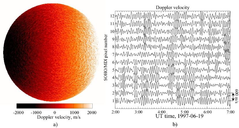
Figure 1: a) Image of the line-of-sight (Doppler) velocity of the solar surface obtained by the Michelson Doppler Imager (MDI) instrument on board SOHO spacecraft on 1997-06-19, 02:00 UT; b) Oscillations of the Doppler velocity, measured by MDI at the solar disk center in 12 CCD pixels separated by $\sim 1.4$ Mm on the Sun.

2 Brief history of helioseismology

Solar oscillations were discovered in 1960 by Robert Leighton, Robert Noyers and George Simon Leighton1962 by analyzing series of Dopplergrams obtained at the Mt. Wilson Observatory. Instead of the expected turbulent behavior of the velocity field they found two distinct classes: large-scale horizontal cellular motions, which they called supergranulation, and vertical quasi-periodic oscillations with a period of about 300 seconds (5 min) and a velocity amplitude of about 0.4 km s^-1. It turned out that these oscillations are the dominant vertical motion in the lower atmosphere (chromosphere) of the Sun. It is remarkable that they realized the diagnostic potential noting that these oscillations ”offer a new means of determining certain local properties of the solar atmosphere, such as the temperature, the vertical temperature gradient, or the mean molecular weight”. They also pointed out that the oscillations might be excited in the Sun’s granulation layer, and account for a part of the energy transfer from the convection zone into the chromosphere.

This discovery was confirmed by other observers, and for several years it was believed that the oscillations represent transient atmospheric waves excited by granules, small convective cells on the solar surface, $1-2\times 10^{3}$ km in size and $8-10$ min lifetime. The physical nature of the oscillation at that time was unclear. In particular, the questions whether these oscillations are acoustic or gravity waves, and if they represent traveling or standing waves remained unanswered for almost a decade after the discovery.

Pierre Mein Mein1966 applied a two-dimensional Fourier analysis (in time and space) to observational data obtained by John Evans and his colleagues at the Sacramento Peak Observatory in 1962-65. His idea was to decompose the oscillation velocity field into normal modes. He calculated the oscillation power spectrum and investigated the relationship between the period and horizontal wavelength (or frequency-wavenumber diagram). From this analysis he concluded that the oscillations are acoustic waves that are stationary (evanescent) in the solar atmosphere. He also made a suggestion that the horizontal structure of the oscillations may be imposed by the convection zone below the surface.

Mein’s results were confirmed by Edward Frazier Frazier1968 who analyzed high-resolution spectrograms taken at the Kitt Peak National Observatory in 1965. In the wavenumber-frequency diagram he noticed that in addition to the primary 5-min peak peak there is a secondary lower frequency peak, which was a new puzzle.

This puzzle was solved by Roger Ulrich Ulrich1970 who following the ideas of Mein and Frazier, calculated the spectrum of standing acoustic waves trapped in a layer below the photosphere. He found that these waves may exist only along discrete line in the wavenumber-frequency ($k-\omega$) diagram, and that the two peaks observed by Frazier correspond to the first two harmonics (normal modes). He formulated the conditions for observing the discrete acoustic modes: observing runs must be longer longer one hour, must cover a sufficiently large region of, at least, 60,000 km in size; the Doppler velocity images must have a spatial resolution of 3,000 km, and be taken at least every 1 minute.

At that time the observing runs were very short, typically, 30-40 min. Only in 1974-75 Franz-Ludwig Deubner Deubner1975 was able to obtain three 3-hour sets of observations using a magnetograph of the Fraunhofer Institute in Anacapri. He measured Doppler velocities along a $\sim 220,000$ km line on the solar disk by scanning it periodically at 110 sec intervals with the scanning steps of about 700 km. The Fourier analysis of these data provided the frequency-wavenumber diagram with three or four mode ridges in the oscillation power spectrum that represents the squared amplitude of the Fourier components as a function of wavenumber and frequency. Deubner’s results provided unambiguous confirmation of the idea that the 5-min oscillations observed on the solar surface represent the standing waves or resonant acoustic modes trapped below the surface. The lowest ridge in the diagram is easily identified as the surface gravity wave because its frequencies depend only on the wavenumber and surface gravity. The ridge above is the first acoustic mode, a standing acoustic waves that have one node along the radius. The ridge above this corresponds to the second acoustic modes with two nodes, and so on.

While these observations showed a remarkable qualitative agreement with Ulrich’s theoretical prediction, the observed power ridges in the $k-\omega$ diagram were systematically lower than the theoretical mode lines. Soon after, in 1975, Edward Rhodes, Ulrich and Simon Rhodes1977 made independent observations at the vacuum solar telescope at the Sacramento Peak Observatory and confirmed the observational results. They also calculated the theoretical mode frequencies for various solar models, and by comparing these with the observations determined the limits on the depth of the solar convection zone. This, probably, was the first helioseismic inference.

However, it was believed that the acoustic (p) modes do not provide much information about the solar interior because detailed theoretical calculations of their properties by Hiroyashi Ando and Yoji Osaki Ando1977 showed that while these mode are determined by interior resonances their amplitude (eigenfunctions) is predominantly concentrated close to the surface. Therefore, the main focus was shifted to observations and analysis of global oscillations of the Sun with periods much longer than 5 min. This task was particularly important for explaining the observed deficit of high-energy solar neutrinos Bahcall1969 , which could be either due to a low temperature (or heavy element abundance - low metallicity) in the energy-generating core or neutrino oscillations.

In 1975, Henry Hill, Tuck Stebbins and Tim Brown Hill1975 reported on the detection of oscillations in their measurements of solar oblateness. The periods of these oscillations were between 10 and 40 min. They suggested that the oscillation signals might correspond to global modes of the Sun. Independently, in 1976, two groups, led by Andrei Severny at the Crimean Observatory Severny1976 and George Isaak at the University of Birmingham Brookes1976 found long-period oscillations in global-Sun Doppler velocity signals. The oscillation with a period of 160 min was particularly prominent and stable. The amplitude of this oscillation was estimated close to 2 m/s. Later this oscillation was found in observations at the Wilcox Solar Observatory Scherrer1979 and at the geographical South Pole Grec1980 . Despite significant efforts to identify this oscillation among the solar resonant modes or to find a physical explanation these results remain a mystery. This oscillations lost the amplitude and coherence in the subsequent ground-based measurements and was not found in later observations from SOHO spacecraft Pall'e1998 . The period of this oscillation was extremely close to 1/9 of a day, and likely was related to terrestrial observing conditions.

Nevertheless, these studies played a very important role in development of helioseismology and emphasized the need for long-term stable and high-accuracy observations from the ground and space. Attempts to detect long-period oscillations (g-modes) still continue. However, the focus of helioseismology was shifted to accurate measurements and analysis of the acoustic p-modes discovered by Leighton.

The next important step was made in 1979 by the Birmingham group Claverie1979 . They observed the Doppler velocity variations integrated over the whole Sun for about 300 hours (but typically 8 hours a day) at two observatories, Izana, on Tenerife, and Pic du Midi in the Pyrenees. In the power spectrum of 5-min oscillations they detected several equally space lines corresponding to global (low-degree) acoustic modes, radial, dipole and quadrupole. (In terms of the angular degree these are labeled as $\ell=0,1,$ and 2). Unlike, the previously observed local short horizontal wavelength acoustic modes these oscillations propagate into the deep interior and provide information about the structure of the solar core. The estimated frequency spacing between the modes was 67.8 $\mu$Hz. This uniform spacing predicted theoretically by Yuri Vandakurov Vandakurov1968 in the framework of a general stellar oscillation theory corresponds to the inverse time that takes for acoustic waves to travel from the surface of the Sun through the center to the opposite side and come back. Thus, the frequency spacing immediately gives an important constraint on the internal structure of the Sun. A comparison with the solar models Iben1976 ; Christensen-Dalsgaard1979 showed that the observed spectrum is consistent with the spectrum of solar models with low metallicity. This result was very exciting because if correct it would provide a solution to the solar neutrino problem. Thus, the determination of solar metallicity (or heavy element abundance) became a central problem of helioseismology.

In the same year, 1974, Gerald Grec, Eric Fossat, and Martin Pomerantz Grec1980 made 5-day continuous measurements at the Amundsen-Scott Station at the South Pole of the global oscillations and confirmed the Birmingham result. Also, they were able to resolve the fine structure of the oscillation spectrum and in addition to the main 67.8 $\mu$Hz spacing (large frequency separation) between the strongest peaks of $\ell=1$ and 2, observe a small 10-16 $\mu$Hz splitting (small separation) between the $\ell=0$ and 2, and $\ell=1$ and 3 modes. The small separation is mostly sensitive to the central part of the Sun and provides additional diagnostic power.

The comparison of the observed oscillation peaks in the frequency power spectra with the p-mode frequencies calculated for solar models showed that below the surface these oscillations correspond to the standing waves with a large number of nodes along the radius (or high radial order). The number of nodes is between 10 and 35, and it was difficult to determine the precise numbers for the observed modes. This created an uncertainty in the helioseismic determination of the heavy element abundance. Joergen Christensen-Dalsgaard and Douglas Gough Christensen-Dalsgaard1981 pointed out that while the South Pole and new Birmingham data favor solar models with normal metallicity the low metallicity models cannot be ruled out.

The uncertainty was resolved three years later in 1983 when Tom Duvall and Jack Harvey Duvall1983 analyzed the Doppler velocity data measured with a photo-diode array in 200 positions along the North-South direction on the disk, and obtained the diagnostic $k-\omega$ diagram for acoustic modes of degree $\ell$, from 1 to 110. This allowed them to connect in the diagnostic diagram the global low-$\ell$ modes with the high-$\ell$ observed by Deubner. Since the correspondence of the ridges on Deubner’s diagram to solar oscillation modes have been determined it was easy to identify the low-$\ell$ modes by simply counting the ridges corresponding to the low-$\ell$ frequencies. It turned out that the these modes are indeed in the best agreement with the normal metallicity solar model. This result had important implications for the solar neutrino problem because it strongly indicated that the observed deficit of solar neutrinos was not due to a low abundance of heavy elements on the Sun but because of changes in neutrino properties (neutrino oscillations) on their way from the energy-generating core to the Earth. This was later confirmed by direct measurements of solar neutrino properties Ahmad2002a .

It was also important that the definite identification of the observed solar oscillations in terms of normal oscillation modes provided a solid foundation for developing diagnostic methods of helioseismology based on the well-developed mathematical theory of non-radial oscillations of stars Pekeris1938 ; Cowling1941 ; Ledoux1958 . This theory provided means for calculating eigenfrequencies and eigenfunctions of normal modes for spherically symmetric stellar models. Mathematically, the problem is reduced to solving a non-linear eigenvalue problem for a fourth-order system of differential equations. This system has two sequences of eigenvalues corresponding to p- and g-modes, and also a degenerate solution, corresponding to f-modes (surface gravity waves). The effects of rotation, asphericity and magnetic fields are usually small and considered by a perturbation theory Gough1990 ; Dziembowski1984 ; Dziembowski1989 ; Dziembowski2005 .

An important prediction of the oscillation theory is that rotation causes splitting of normal mode frequencies. Without rotation, the normal mode frequencies are degenerate with respect to the azimuthal wavenumber, $m$, that is the modes of the angular degree, $l$, and radial order, $n$, have the same frequencies irrespective of the azimuthal (longitudinal) wavelength. The stellar rotation removes this degeneracy. Obviously, it does not affect the axisymmetrical ($m$=0) modes, but the frequencies of non-axisymmetrical modes are split. Generally, these modes can be represented as a superposition of two waves running around a star in two opposite directions (prograde and retrograde waves). Without rotation, these modes have the same frequencies and, thus, the same phase speed. In this case, they form a standing wave. However, rotation increases the speed of the prograde wave and decreases the speed of retrograde wave. This results in an increase of the eigenfrequency of the prograde mode, and a frequency decrease of the retrograde mode. This phenomenon is similar to frequency shifts due to the Doppler effect. It is called rotational frequency splitting.

The rotational frequency splitting was first observed by Ed Rhodes, Roger Ulrich and Franz Deubner Rhodes1979 ; Ulrich1979 ; Deubner1979 . These measurements provided first evidence that the rotation rate of the Sun is not uniform but increases with depth. The rotational splitting was initially measured for high-degree modes, but then the measurements were extended to medium- and low-degree range by Tom Duvall and Jack Harvey Duvall1984 ; Duvall1984a , who made a long continuous series of helioseismology observations at the South Pole. The internal differential rotation law was determined from the data of Tim Brown and Cherilynn Morrow Brown1987 . It was found that the differential latitudinal rotation is confined in the convection zone, and that the radiative interior rotates almost uniformly, and also slower in the equatorial region than the convective envelope Kosovichev1988 ; Brown1989 . Such rotation law was not expected from theories of stellar rotation, which predicted that the stellar cores rotate faster than the envelopes Rosner1985 . The knowledge of the Sun’s internal rotation law is of particular importance for understanding the dynamo mechanism of magnetic field generation Parker1993 .

It became clear that for long uninterrupted observations are essential for accurate inferences of the internal structure and rotation of the Sun. Therefore, the observational programs focused on development of global helioseismology networks, GONG Harvey1988 and BiSON Brookes1978 ; Isaak1989 , and also the Solar and Heliospheric Observatory (SOHO) space mission Domingo1995 . These projects provided almost continuous coverage for helioseismic observations and also stimulated development of new sophisticated data analysis and inversion techniques.

In addition, the Michelson Doppler Imager (MDI) instrument on SOHO Scherrer1995 and the GONG+ network upgraded to higher spatial resolution Leibacher2003 provided excellent opportunities for developing local helioseismology, which provides tools for three-dimensional imaging of the solar interior. The local helioseismology methods are based on measurements of local oscillation properties, such as frequency shift in local areas or variations of travel times.

The idea of using the local frequency shifts for inferring the subsurface flows was suggested by Douglas Gough and Juri Toomre in 1983 Gough1983 . The method is now called ring-diagram analysis Hill1988 , because the dispersion relation of solar oscillations forms rings in horizontal wavenumber plane at a given frequency. It measures shifts of these rings, which are then converted into frequency shifts. Ten years later, Tom Duvall and his colleagues Duvall1993 introduced time-distance helioseismology method. In this method, they suggested to measure travel times of acoustic waves from a cross-covariance function of solar oscillations. This function is obtained by cross-correlating oscillation signals observed at two different points on the solar surface for various time lags. When the time lag in the calculations coincides with the travel time of acoustic waves between these points the cross-covariance function shows a maximum. This method provided means for developing acoustic tomography techniques Kosovichev1996 ; Kosovichev1997 for imaging 3D structures and flows with the high-resolution comparable to the oscillation wavelength. These and other methods of local area helioseismology Chang1997 ; Lindsey2000 have provided important results on the convective and large-scale flows, and also on the structure and evolution of sunspots and active regions. Their development continues.

The SOHO mission and the GONG network were primarily designed for observing solar oscillation modes of low- and medium-degree, needed for global helioseismology. Local helioseismology requires high-resolution observations of high-degree modes. Because of the telemetry constraints such data are available uninterruptedly from the MDI instrument on SOHO only for 2 months every year. These data provided only snapshots of the subsurface structures and dynamics associated with the solar activity. In order to fully investigate the evolving magnetic activity of the Sun, a new space mission Solar Dynamics Observatory (SDO) was launched on February 11, 2010. It carries Helioseismic and Magnetic Imager (HMI) instrument, which will provide continuous 4096x4096-pixel full-disk images of solar oscillations. These data will open new opportunities for investigation the solar interior by local helioseismology Kosovichev2007a .

In the modern helioseismology, a very important role is played by numerical simulations. Both, global and local helioseismology analysis employ relatively simple for fitting the observational data and performing inversions of the fitted frequencies and travel times. For instance, the global helioseismology methods assume that the structures and flows on the Sun are axisymmetrical and infer only the axisymmetrical components of the sound speed and velocity field. The local helioseismology methods are based on a simplified physics of wave propagation on the Sun. The ring-diagram analysis makes an assumption that that the perturbations and flows are horizontally uniform within the area used for calculating the wave dispersion relation, 5-15 heliographic degrees, while a typical size of sunspots is about 1-2 degrees. Most of the time-distance helioseismology inversions are based on a ray-path approximation and ignore the finite wavelength effects that become important at small scales, comparable with the wavelength. Also, all the methods, global and local, do not take into account many effects of solar magnetic fields. Properties of solar oscillations dramatically change in regions of strong magnetic field. In particular, the excitation of oscillations is suppressed in sunspots because the strong magnetic field inhibits convection that drives the oscillations. The magnetic stresses may cause anisotropy of wave speed and lead to transformation of acoustic waves into various MHD type waves. These and other effects have to be investigated and taken into account in the data analysis and inversion procedures. Because of the complexity, these processes can be fully investigated only numerically. The numerical simulations of subsurface solar convection and oscillations were pioneered by Robert Stein and Åke Nordlund Stein1989 . These 3D radiative MHD simulations include all essential physics and provide important insights into the physical processes below the visible surface and also artificial data for helioseismology testing. This type of so-called ”realistic” simulations has been used for testing time-distance helioseismology inferences Zhao2007 , and continues being developed using modern turbulence models Jacoutot2008 . In addition, for testing various aspects of wave propagation and interaction with magnetic fields are studied by solving numerically linearized MHD equations (e.g. Hanasoge2007 ; Parchevsky2008 ; Hartlep2008 ). The numerical simulations become an important tool for verification and testing of the helioseismology methods and inferences.

3 Basic properties of solar oscillations

3.1 Oscillation power spectrum

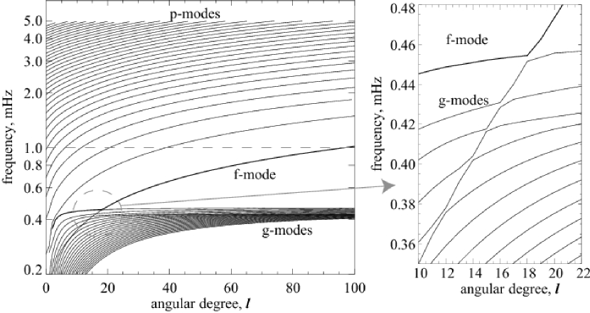
Figure 2: Theoretical frequencies of solar oscillation modes calculated for a standard solar model for a range of angular degree $l$ from 0 to 100, and for the frequency range from 0.2 mHz to 5 mHz. The solid curves connect modes corresponding to the different oscillation overtones (radial orders) The dashed grey horizontal line indicate the low-frequency observational limit: only the modes above this line have been reliably observed. The right panel shows an area of the avoided crossing of f- and g-modes (indicated by the gray dashed circle in left panel).

The theoretical spectrum of solar oscillation modes shown in Fig. 2 covers a wide range of frequencies and angular degrees. It includes oscillations of three types: acoustic (p) modes, surface gravity (f) modes and internal gravity (g) modes. In this spectrum, the modes are organized a series of curves corresponding to different overtones of non-radial modes, which are characterized by the number of nodes along the radius (or by the radial order, $n$). The angular degree, $l$, of the corresponding spherical harmonics describes the horizontal wave number (or inverse horizontal wavelength). The p-modes cover the frequency range from 0.3 to 5 mHz (or from 3 to 55 min in oscillation periods). The low frequency limit corresponds to the first radial harmonic, and the upper limit is set by the acoustic cut-off frequency of the solar atmosphere. The g-modes frequencies have an upper limit corresponding to the maximum Brünt-Väisälä frequency ($\sim 0.45$ mHz) in the radiative zone and occupy the low-frequency part of the spectrum. The intermediate frequency range of 0.3-0.4 mHz at low angular degrees is a region of mixed modes. These modes behave like g-modes in the deep interior and like p-modes in the outer region. The apparent crossings in this diagram are not the actual crossings: the mode branches become close in frequencies but do not cross each other. At these points the mode exchange their properties, and the mode branches are diverted. For instance, the f-mode ridge stays above the g-mode lines. A similar phenomenon is known in quantum mechanics as avoided crossing.

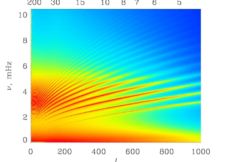
Figure 3: Power spectrum obtained from a 6-day long time series of solar oscillation data from the MDI instrument on SOHO in 1996 ($\nu$ is the cyclic frequency of the oscillations, $l$ is the angular degree, $\lambda_{h}$ is the horizontal wavelength in megameters).

So far, only the upper part of the solar oscillation spectrum is observed. The lowest frequencies of detected p- and f-modes are of about 1 mHz. At lower frequencies the mode amplitudes decrease below the noise level, and become unobservable. There have been several attempts to identify low-frequency p-modes or even g-modes in the noisy spectrum, but so far these results are not convincing.

The observed power spectrum is shown in Fig. 3. The lowest ridge is the f-mode, and the other ridges are p-modes of the radial order, $n$, starting from $n=1$. The ridges of the oscillation modes disappear in the convective noise at frequencies below 1 mHz. The power spectrum is obtained from the SOHO/MDI data, representing 1024x1024-pixel images of the line-of-sight (Doppler) velocity of the solar surface taken every minute without interruption. When the oscillations are observed in the integrated solar light (”Sun-as-a-star”) then only the modes of low angular degree are detected in the power spectrum (Fig. 4). These modes have a mean period of about 5 min, and represent p-modes of high radial order $n$ modes. The $n$-values of these modes can be determined by tracing in Fig. 3 the the high-$n$ ridges of the high-degree modes into the low-degree region. This provides unambiguous identification of the low-degree solar modes. Obviously, the mode identification is much more difficult for spatially unresolved oscillations of other stars.

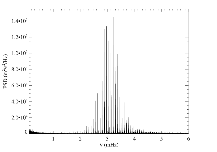
Figure 4: Power spectral density (PSD) of low-degree solar oscillations, obtained from the integrated light observations (Sun-as-a-star) by the GOLF instrument on SOHO, from 11/04/1996 to 08/07/2008.

3.2 Excitation by turbulent convection

Observations and numerical simulations have shown that solar oscillations are driven by turbulent convection in a shallow subsurface layer with a superadiabatic stratification, where convective velocities are the highest. However, details of the stochastic excitation mechanism are not fully established. Solar convection in the superadiabatic layer forms small-scale granulation cells. Analysis of the observations and numerical simulations has shown that sources of solar oscillations are associated with strong downdrafts in dark intergranular lanes Rimmele1995 . These downdrafts are driven by radiative cooling and may reach near-sonic velocity of several km/s. This process has features of convective collapse Skartlien2000 .

Calculations of the work integral for acoustic modes using the realistic numerical simulations of Stein and Nordlund Stein2001 have shown that the principal contribution to the mode excitation is provided by turbulent Reynolds stresses and that a smaller contribution comes from non-adiabatic pressure fluctuations. Because of the very high Reynolds number of the solar dynamics the numerical modeling requires an accurate description of turbulent dissipation and transport on the numerical subgrid scale. The recent radiative hydrodynamics modeling using the Large-Eddy Simulations (LES) approach and various subgrid scale (SGS) formulations Jacoutot2008 showed that among these formulations the most accurate description in terms of the reproducing the total amount of the stochastic energy input to the acoustic oscillations is provided by a dynamic Smagorinsky model Germano1991 ; Moin1991 (Fig. 5a).

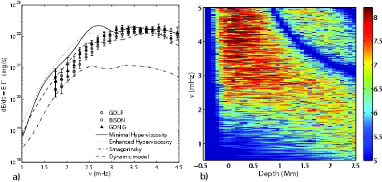
Figure 5: a) Comparison of observed and calculated rate of stochastic energy input to modes for the entire solar surface ($erg\;s^{-1}$). Different curves show the numerical simulation results obtained for 4 turbulence models: hyperviscosity (solid), enhanced hyperviscosity (dots), Smagorinsky (dash-dots), and dynamic model (dashes). Observed distributions: $circles$ SoHo-GOLF, $squares$ BISON, and $triangles$ GONG for $l=1$ Baudin2005 . b) Logarithm of the work integrand in units of $erg\;cm^{-2}\;s^{-1}$), as a function of depth and frequency for numerical simulations with the dynamic turbulence model Jacoutot2008a .

As we have pointed out, the observations show that the modal lines in the oscillation power spectrum are not Lorentzian but display a strong asymmetry Duvall1993a ; Toutain1998 . Curiously, the asymmetry has the opposite sense in the power spectra calculated from Doppler velocity and intensity oscillations. The asymmetry itself can be easily explained by interference of waves emanated by a localized source Gabriel1992 , but the asymmetry reversal is surprising and indicates complicated radiative dynamics of the excitation process. The reversal has been attributed to a correlated noise contribution to the observed intensity oscillations Nigam1998 , but the physics of this effect is still not fully understood. However, it is clear that the line shape of the oscillation modes and the phase-amplitude relations of the velocity and intensity oscillations carry substantial information about the excitation mechanism and, thus, require careful data analysis and modeling.

3.3 Line asymmetry and pseudo-modes

Figure 6 shows the power spectrum for oscillations of the angular degree, $l=200$, obtained from the SOHO/MDI Doppler velocity and intensity data Nigam1998 . The line asymmetry is apparent, particularly, at low frequencies. In the velocity spectrum, there is more power in the low-frequency wings than in the high-frequency wings of the spectral lines. In the intensity spectrum, the distribution of power is reversed. The data also show that the asymmetry varies with frequency. It is the strongest for the f-mode and low-frequency p-mode peaks. At higher frequencies the peaks become more symmetrical, and extend well above the acoustic cut-off frequency (Eq. 51), which is $\sim 5-5.5$ mHz.

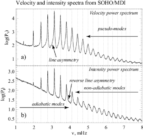
Figure 6: Power spectra of $l=200$ modes obtained from SOHO/MDI observations of a) Doppler velocity, b) continuum intensity Nigam1998 .

Acoustic waves with frequencies below the cut-off frequency are completely reflected by the surface layers because of the steep density gradient. These waves are trapped in the interior, and their frequencies are determined by the resonant conditions, which depend on the solar structure. But the waves with frequencies above the cut-off frequency escape into the solar atmosphere. Above this frequency the power spectrum peaks correspond to so-called ”pseudo-modes”. These are caused by constructive interference of acoustic waves excited by the sources located in the granulation layer and traveling upward, and by the waves traveling downward, reflected in the deep interior and arriving back to the surface. Frequencies of these modes are no longer determined by the resonant conditions of the solar structure. They depend on the location and properties of the excitation source (”source resonance”). The pseudo-mode peaks in the velocity and intensity power spectra are shifted relative to each other by almost a half-width. They are also slightly shifted relative to the normal mode peaks although they look like a continuation of the normal-mode ridges in Figs 1b and 4a. This happens because the excitation sources are located in a shallow subsurface layer, which is very close to the reflection layers of the normal modes. Changes in the frequency distributions below and above the acoustic cut-off frequency can be easily noticed by plotting the frequency differences along the modal ridges.

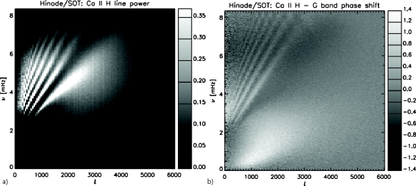
Figure 7: a) The oscillation power spectrum from Hinode CaII H line observations. b) The phase shift between CaII H and G-band (units are in radians) Mitra-Kraev2008 .

The asymmetrical profiles of normal-mode peaks are also caused by the localized excitation sources. The interference signal between acoustic waves traveling from the source upwards and the waves traveling from the source downward and coming back to the surface after the internal reflection depends on the wave frequency. Depending on the multipole type of the source the interference signal can be stronger at frequencies lower or higher than the resonant normal frequencies, thus resulting in asymmetry in the power distribution around the resonant peak. Calculations of Nigam et al. Nigam1998 showed that the asymmetry observed in the velocity spectra and the distribution of the pseudo-mode peaks can be explained by a composite source consisting of a monopole term (mass term) and a dipole term (force due to Reynolds stress) located in the zone of superadiabatic convection at a depth of $\simeq 100$ km below the photosphere. In this model, the reversed asymmetry in the intensity power spectra is explained by effects of a correlated noise added to the oscillation signal through fluctuations of solar radiation during the excitation process. Indeed, if the excitation mechanism is associated with the high-speed turbulent downdrafts in dark lanes of granulation the local darkening contributes to the intensity fluctuations caused by excited waves. The model also explains the shifts of pseudo-mode frequency peaks and their higher amplitude in the intensity spectra. The difference between the correlated and uncorrelated noise is that the correlated noise has some phase coherence with the oscillation signal, while the uncorrelated noise has no coherence.

While this scenario looks plausible and qualitatively explains the main properties of the power spectra details of the physical processes are still uncertain. In particular, it is unclear whether the correlated noise affects only the intensity signal or both the intensity and velocity. It has been suggested that the velocity signal may have a correlated contribution due to convective overshoot Roxburgh1997 . Attempts to estimate the correlated noise components from the observed spectra have not provided conclusive results Severino2001 ; Wachter2005 . Realistic numerical simulations Georgobiani2003 have reproduced the observed asymmetries and provided an indication that radiation transfer plays a critical role in the asymmetry reversal.

Recent high-resolution observations of solar oscillation simultaneously in two intensity filters, in molecular G-band and CaII H line, from the Hinode space mission Kosugi2007 ; Tsuneta2008 revealed significant shifts in frequencies of pseudo-modes observed in the CaII H and G-band intensity oscillations Mitra-Kraev2008 . The phase of the cross-spectrum of these oscillations shows peaks associated with the p-mode lines but no phase shift for the f-mode (Fig. 7b). The p-mode properties can be qualitatively reproduced in a simple model with a correlated background if the correlated noise level in the Ca II H data is higher than in the G-band data Mitra-Kraev2008 . Perhaps, the same effect can explain also the frequency shift of pseudo-modes. The CaII H line is formed in the lower chromosphere while the G-band signal comes from the photosphere. But how this may lead to different levels of the correlated noise is unclear.

The Hinode results suggest that multi-wavelength observations of solar oscillations, in combination with the traditional intensity-velocity observations, may help to measure the level of the correlated background noise and to determine the type of wave excitation sources on the Sun. This is important for understanding the physical mechanism of the line asymmetry and for developing more accurate models and fitting formulae for determining the mode frequencies Nigam1998a .

In addition, Hinode provided observations of non-radial acoustic and surface gravity modes of very high angular degree. These observations show that the oscillation ridges are extended up to $l\simeq 4000$ (Fig. 7a). In the high-degree range, $l\geq 2500$ frequencies of all oscillations exceed the acoustic cut-off frequency. The line width of these oscillations dramatically increases, probably due to strong scattering on turbulence Duvall1998 ; Murawski1998 . Nevertheless, the ridge structure extending up to 8 mHz (Nyquist frequency of these observations) is quite clear. Although the ridge slope clearly changes at the transition from the normal modes to the pseudo-modes.

3.4 Magnetic effects: sunspot oscillations and acoustic halos

In general, the main factors causing variations in oscillation properties in magnetic regions, can be divided in two types: direct and indirect. The direct effects are due to additional magnetic restoring forces that can change the wave speed and may transform acoustic waves into different types of MHD waves. The indirect effects are caused by changes in convective and thermodynamic properties in magnetic regions. These include depth-dependent variations of temperature and density, large-scale flows, and changes in wave source distribution and strength. Both direct and indirect effects may be present in observed properties such as oscillation frequencies and travel times, and often cannot be easily disentangled by data analyses, causing confusions and misinterpretations. Also, one should keep in mind that simple models of MHD waves derived for various uniform magnetic configurations and without stratification or with a polytropic stratification may not provide correct explanations to solar phenomena. In this situation, numerical simulations play an important role in investigations of magnetic effects.

Observed changes of oscillation amplitude and frequencies in magnetic regions are often explained as a result of wave scattering and conversion into various MHD modes. However, recent numerical simulations helped us to understand that magnetic fields not only affect the wave dispersion properties but also the excitation mechanism. In fact, changes in excitation properties of turbulent convection in magnetic regions may play a dominant role in observed phenomena.

Sunspot oscillations

For instance, it is well-known that the amplitude of 5-min oscillations is substantially reduced in sunspots. Observations show that more waves are coming into the sunspot than going out of the sunspot area (e.g. Braun1987 ). This is often attributed to absorption of acoustic waves in magnetic field due to conversion into slow MHD modes traveling along the field lines (e.g. Cally2009 ). However, since convective motions are inhibited by the strong magnetic field of sunspots, the excitation mechanism is also suppressed. Three-dimensional numerical simulations of this effect have shown that the reduction of acoustic emissivity can explain at least 50% of the observed power deficit in sunspots (Fig. 8) Parchevsky2007a .

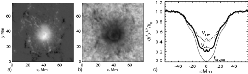
Figure 8: a) Line-of-sight magnetic field map of a sunspot (AR8243); b) oscillation amplitude map; c) profiles of rms oscillation velocities at frequency 3.65 mHz for observations (thick solid curves) and simulations (dashed curves); the thin solid curve shows the distribution of the simulated source strength Parchevsky2007a .

Another significant contribution comes from the amplitude changes caused by variations in the background conditions. Inhomogeneities in the sound speed may increase or decrease the amplitude of acoustic wave traveling through these inhomogeneities. Numerical simulations of MHD waves using magnetostatic sunspot models show that the amplitude of acoustic waves traveling through sunspot decreases when the wave is inside sunspot and then increases when the wave comes out of sunspot Parchevsky2010 . Simulations with multiple random sources show that these changes in the wave amplitude together with the suppression of acoustic sources can explain the whole observed deficit of the power of 5-min oscillations. Thus, the role of the MHD mode conversion may be insignificant for explaining the power deficit of 5-min photospheric oscillations in sunspots. However, the mode conversion is expected to be significant higher in the solar atmosphere where magnetic forces become dominant.

We should note that while the 5-min oscillations in sunspots come mostly from outside sources there are also 3-min oscillations, which are probably intrinsic oscillations of sunspots. The origin of these oscillations is not yet understood. They are probably excited by a different mechanism operating in strong magnetic field.

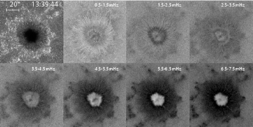
Figure 9: CaII H intensity image from Hinode observations (top-left) and the corresponding power maps from CaII H intensity data in five frequency intervals of active region NOAA 10935. The field of view is 100 arcsec square in all the panels. The power is displayed in logarithmic greyscaling Nagashima2007 .

Hinode observations added new puzzles to sunspot oscillations. Figure 9 shows a sample Ca II H intensity and the relative intensity power maps averaged over 1 mHz intervals in the range from 1 mHz to 7 mHz with logarithmic greyscaling Nagashima2007 . In the Ca II H power maps, in all the frequency ranges, there is a small area ($\sim$ 6 arcsec in diameter) near the center of the umbra where the power was suppressed. This type of ‘node’ has not been reported before. Possibly, the stable high-resolution observation made by Hinode/SOT was required to find such a tiny node, although analysis of other sunspots indicates that probably only a particular type of sunspots, e.g., round ones with axisymmetric geometry, exhibit such node-like structure. Above 4 mHz in the Ca II H power maps, power in the umbra is remarkably high. In the power maps averaged over narrower frequency range (0.05 mHz wide, not shown), the region with high power in the umbra seems to be more patchy. This may correspond to elements of umbral flashes, probably caused by overshooting convective elements Schussler2006 . The Ca II H power maps show a bright ring in the penumbra at lower frequencies. It probably corresponds to the running penumbral waves. The power spectrum in the umbra has two peaks: one around 3 mHz and the other around 5.5 mHz. The high-frequency peak is caused by the oscillations that excited only in the strong magnetic field of sunspots. The origin of these oscillations is not known yet.

Acoustic halos

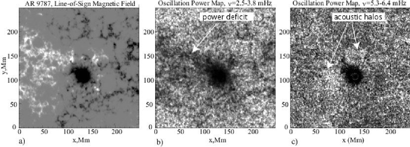
Figure 10: a) Line-of-sight magnetic field map of active region NOAA 9787 observed from SOHO/MDI on Jan. 24, 2002 and averaged over a 3-hour period; b) oscillation power map from Doppler velocity measurements for the same period in the frequency 2.5–3.8 mHz; c) power map for 5.3–6.4 mHz.

In moderate field regions, such as plages around sunspot regions, observations reveal enhanced emission at high frequencies, 5-7 mHz, (with period $\sim 3$ min) Braun1992 . Sometimes this emission is called the ”acoustic halo” (Fig. 10c). There have been several attempts to explain this effect as a result of wave transformation or scattering in magnetic structures (e.g. Hanasoge2008 ; Khomenko2009 ). However, numerical simulations show that magnetic field can change the excitation properties of solar granulation resulting in an enhanced high-frequency emission. In particular, the radiative MHD simulations of solar convection Jacoutot2008a in the presence of vertical magnetic field have shown that the magnetic field significantly changes the structure and dynamics of granulations, and thus the conditions of wave excitation. In magnetic field the granules become smaller, and the turbulence spectrum is shifted towards higher frequencies. This is illustrated in Figure 11, which shows the frequency spectrum of the horizontally averaged vertical velocity. Without a magnetic field the turbulence spectrum declines sharply at frequencies above 5 mHz, but in the presence of magnetic field it develops a plateau. In the plateau region characteristic peaks (corresponding to the ”pseudo-modes”) appear in the spectrum for moderate magnetic field strength of about 300-600 G. These peaks may explain the effect of the ”acoustic halo”. Of course, more detailed theoretical and observational studies are required to confirm this mechanism. In particular, multi-wavelength observations of solar oscillations at several different heights would be important. Investigations of the excitation mechanism in magnetic regions is also important for interpretation of the variations of the frequency spectrum of low-degree modes on the Sun, and for asteroseismic diagnostics of stellar activity.

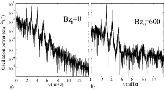
Figure 11: Power spectra of the horizontally averaged vertical velocity at the visible surface for different initial vertical magnetic fields. The peaks on the top of the smooth background spectrum of turbulent convection represent oscillation modes: the sharp asymmetric peaks below 6 mHz are resonant normal modes, while the broader peaks above 6 mHz, which become stronger in magnetic regions, correspond to pseudo-modes.Jacoutot2008a

3.5 Impulsive excitation: sunquakes

“Sunquakes”, the helioseismic response to solar flares, are caused by strong localized hydrodynamic impacts in the photosphere during the flare impulsive phase. The helioseismic waves have been observed directly as expanding circular-shaped ripples in SOHO/MDI Dopplergrams Kosovichev1998 (Fig. 12).

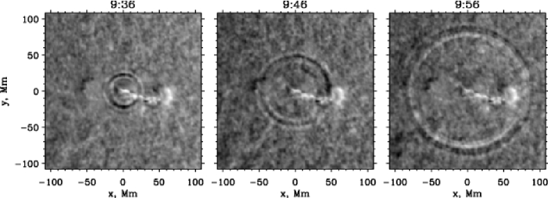
Figure 12: Observations of the seismic response (“sunquakes”) of the solar flare of 9 July, 1996, showing a sequence of Doppler-velocity images, taken by the SOHO/MDI instrument. The signal of expanding ripples is enhanced by a factor 4 in the these images.

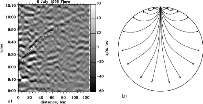
Figure 13: a) The time-distance diagram of the seismic response to the solar flare of 9 July, 1996. b) Illustration of acoustic ray paths of the flare-excited waves traveling through the Sun.

These waves can be detected in Dopplergram movies and as a characteristic ridge in time-distance diagrams (Fig. 13a), Kosovichev1998 ; Kosovichev2006a ; Kosovichev2006b ; Kosovichev2006c , or indirectly by calculating integrated acoustic emission Donea1999 ; Donea2005 ; Donea2006 . Solar flares are sources of high-temperature plasma and strong hydrodynamic motions in the solar atmosphere. Perhaps, in all flares such perturbations generate acoustic waves traveling through the interior. However, only in some flares is the impact sufficiently localized and strong to produce the seismic waves with the amplitude above the convection noise level. It has been established in the initial July 9, 1996, flare observations Kosovichev1998 that the hydrodynamic impact follows the hard X-ray flux impulse, and hence, the impact of high-energy electrons.

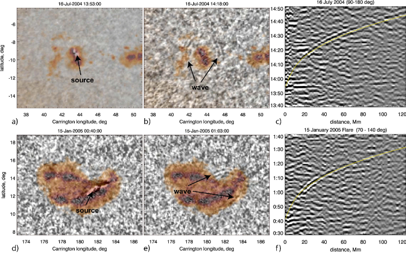
Figure 14: Observations of the seismic response of the Sun (“sunquakes”) to two solar flares: a-c) X3 of 16 July, 2004, and d-f) X1 flare of 15 January, 2005. The left panels show a superposition of MDI white-light images of the active regions and locations of the sources of the seismic waves determined from MDI Dopplergrams, the middle column shows the seismic waves, and the right panels show the time-distance diagrams of these events. The thin yellow curves in the right panels represent a theoretical time-distance relation for helioseismic waves for a standard solar model.Kosovichev2006c

A characteristic feature of the seismic response in this flare and several others Kosovichev2006a ; Kosovichev2006b ; Kosovichev2006c is anisotropy of the wave front: the observed wave amplitude is much stronger in one direction than in the others. In particular, the seismic waves excited during the October 28, 2003, 16 July, 2004, flare of 15 January, 2005 flare had the greatest amplitude in the direction of the expanding flare ribbons (Fig. 14). The wave anisotropy can be attributed to the moving source of the hydrodynamic impact, which is located in the flare ribbons Kosovichev2006a ; Kosovichev2006c ; Kosovichev2007 . The motion of flare ribbons is often interpreted as a result of the magnetic reconnection processes in the corona. When the reconnection region moves up it involves higher magnetic loops, the footpoints of which are further apart. The motion of the footpoints of impact of the high-energy particles is particularly well observed in the SOHO/MDI magnetograms showing magnetic transients moving with supersonic speed, in some cases Kosovichev2006b . Of course, there might be other reasons for the anisotropy of the wave front, such as inhomogeneities in temperature, magnetic field, and plasma flows. However, the source motion seems to be a key factor.

Therefore, we conclude that the seismic wave was generated not by a single impulse but by a series of impulses, which produce the hydrodynamic source moving on the solar surface with a supersonic speed. The seismic effect of the moving source can be easily calculated by convolving the wave Green’s function with a moving source function. The results of these calculations a strong anisotropic wavefront, qualitatively similar to the observations Kosovichev2007 . Curiously, this effect is quite similar to the anisotropy of seismic waves on Earth, when the earthquake rupture moves along the fault. Thus, taking into account the effects of multiple impulses of accelerated electrons and moving source is very important for sunquake theories. The impulsive sunquake oscillations provide unique information about interaction of acoustic waves with sunspots. Thus, these effects must be studied in more detail.

4 Global helioseismology

4.1 Basic equations

A simple theoretical model of solar oscillations can be derived using the following assumptions:

1. linearity: ${\vec{v}}/c<<1$, where ${\vec{v}}$ is velocity of oscillating elements, $c$ is the speed of sound;

2. adiabaticity: $dS/dt=0$, where $S$ is the specific entropy;

3. spherical symmetry of the background state;

4. magnetic forces and Reynolds stresses are negligible.

The basic governing equations are derived from the conservation of mass, momentum, energy and the Newton’s gravity law. The conservation of mass (continuity equation) assumes that the rate of mass change in a fluid element of volume $V$ is equal to the mass flux through the surface of this element (of area $A$):

$$\frac{\partial}{\partial t}\int_{V}\rho dV=-\int_{A}\rho{\vec{v}}d{\vec{a}}=-\int_{V}\nabla(\rho{\vec{v}})dV,$$ (1)

where $\rho$ is the mass density. Then,

$$\frac{\partial\rho}{\partial t}+\nabla(\rho\vec{v})=0,$$ (2)

or in terms of the material derivative $d\rho/dt=\partial\rho/\partial t+\vec{v}\cdot\nabla\rho$:

$$\frac{d\rho}{dt}+\rho\nabla\vec{v}=0.$$ (3)

The momentum equation (conservation of momentum of a fluid element) is:

$$\rho\frac{d\vec{v}}{dt}=-\nabla P+\rho\vec{g},$$ (4)

where $P$ is pressure, $\vec{g}$ is the gravity acceleration, which can be expressed in terms of gravitational potential $\Phi$: $\vec{g}=\nabla\Phi$, $d\vec{v}/dt=\partial\vec{v}/\partial t+\vec{v}\cdot\nabla\vec{v}$ is the material derivative for the velocity vector. The adiabaticity equation (conservation of energy) for a fluid element is:

$$\frac{dS}{dt}=\frac{d}{dt}\left(\frac{P}{\rho^{\gamma}}\right)=0,$$ (5)

or

$$\frac{dP}{dt}=c^{2}\frac{d\rho}{dt},$$ (6)

where $c^{2}=\gamma P/\rho$ is the squared adiabatic sound speed. The gravitational potential is calculated from the Poisson equation:

$$\nabla^{2}\Phi=4\pi G\rho.$$ (7)

Now, we consider small perturbations of a stationary spherically symmetrical star in hydrostatic equilibrium:

$$v_{0}=0,\;\rho=\rho_{0}(r),\;P=P_{0}(r).$$

If $\vec{\xi}(t)$ is a vector of displacement of a fluid element then velocity $\vec{v}$ of this element:

$$\vec{v}=\frac{d\xi}{dt}\approx\frac{\partial\vec{\xi}}{\partial t}.$$ (8)

Perturbations of scalar variables, $\rho,P,\Phi$ can be of two general types: Eulerian (denoted with prime symbol), at a fixed position $\vec{r}$:

$$\rho(\vec{r},t)=\rho_{0}(r)+\rho^{\prime}(\vec{r},t),$$

and Lagrangian, measured in the moving element (denoted with $\delta$):

$$\delta\rho(\vec{r}+\vec{\xi})=\rho_{0}(r)+\delta\rho(\vec{r},t).$$ (9)

The Eulerian and Lagrangian perturbations are related to each other:

$$\delta\rho=\rho^{\prime}+(\vec{\xi}\cdot\nabla\rho_{0})=\rho^{\prime}+(\vec{\xi}\cdot\vec{e}_{r})\frac{d\rho_{0}}{dr}=\rho^{\prime}+\xi_{r}\frac{d\rho_{0}}{dr},$$ (10)

where $\vec{e}_{r}$ is the radial unit vector.

In terms of the Eulerian perturbations and the displacement vector, $\vec{\xi}$ the linearized mass, momentum and energy equations can be expressed in the following form:

$$\rho^{\prime}+\nabla(\rho_{0}\vec{\xi})=0,$$ (11)

$$\rho_{0}\frac{\partial\vec{v}}{\partial t}=-\nabla P^{\prime}-g_{0}\vec{e}_{r}\rho^{\prime}+\rho_{0}\nabla\Phi^{\prime},$$ (12)

$$P^{\prime}+\xi_{r}\frac{dP_{0}}{dr}=c_{0}^{2}(\rho^{\prime}+\xi_{r}\frac{d\rho_{0}}{dr}),$$ (13)

$$\nabla^{2}\Phi^{\prime}=4\pi G\rho^{\prime}.$$ (14)

The equation of solar oscillations can be further simplified by neglecting the perturbations of the gravitational potential, which give relatively small corrections to theoretical oscillation frequencies. This is so-called Cowling approximation: $\Phi^{\prime}=0.$

Now, we consider the linearized equations in the spherical coordinate system, $r,\theta,\phi$. In this system, the displacement vector has the following form:

$$\vec{\xi}=\xi_{r}\vec{e}_{r}+\xi_{\theta}\vec{e}_{\theta}+\xi_{\phi}\vec{e}_{\phi}\equiv\xi_{r}\vec{e}_{r}+\vec{\xi}_{h},$$ (15)

where $\vec{\xi}_{h}=\xi_{\theta}\vec{e}_{\theta}+\xi_{\phi}\vec{e}_{\phi}$ is the horizontal component of displacement. Also, we use the equation for divergence of the displacement (called dilatation):

$$\nabla\vec{\xi}\equiv{\rm div}\xi= \frac{1}{r^{2}}\frac{\partial}{\partial r}(r^{2}\xi_{r})+\frac{1}{r\sin\theta}\frac{\partial}{\partial\theta}(\sin\theta\xi_{\theta})+\frac{1}{r\sin\theta}\frac{\partial\xi_{\phi}}{\partial\phi}=$$

$$=\frac{1}{r^{2}}\frac{\partial}{\partial r}(r^{2}\xi_{r})+\frac{1}{r}\nabla_{h}\vec{\xi}_{h}.$$ (16)

We consider periodic perturbations with frequency $\omega$: $\vec{\xi}\propto\exp({i\omega t}),...$. Here, $\omega$ is the angular frequency measured in rad/sec; it relates to the cyclic frequency, $\nu$, which measures the number of oscillation cycles per sec, as: $\omega=2\pi\nu$.

Then, in the Cowling approximation, we obtained the following system of the linearized equations (omitting subscript $0$ for unperturbed variables):

$$\rho^{\prime}+\frac{1}{r^{2}}\frac{\partial}{\partial r}(r^{2}\rho\xi_{r})+\frac{\rho}{r}\nabla_{h}\vec{\xi}_{h}=0,$$ (17)

$$-\omega^{2}\rho\xi_{r}=-\frac{\partial P^{\prime}}{\partial r}+g\rho^{\prime},$$ (18)

$$-\omega^{2}\rho\vec{\xi}_{h}=-\frac{1}{r}\nabla_{h}P^{\prime},$$ (19)

$$\rho^{\prime}=\frac{1}{c^{2}}P^{\prime}+\frac{\rho N^{2}}{g}\xi_{r},$$ (20)

where

$$N^{2}=g\left(\frac{1}{\gamma P}\frac{dP}{dr}-\frac{1}{\rho}\frac{d\rho}{dr}\right)$$ (21)

is the Brünt-Väisälä (or buoyancy) frequency.

For the boundary conditions, we assume that the solution is regular at the Sun’s center. This correspond to the zero displacement, $\xi_{r}=0$ at $r=0$, for all oscillation modes except of the dipole modes of angular degree $l=1$. In the dipole-mode oscillations the center of a star oscillates (but not the center of mass), and the boundary condition at the center is replaced by a regularity condition. At the surface, we assume that the Lagrangian pressure perturbation is zero: $\delta P=0$ at $r=R$. This is equivalent to the absence of external forces. Also, we assume that the solution is regular at the poles $\theta=0,\pi$.

We seek a solution of Eqs (17-20) by separation of the radial and angular variables in the following form:

$$\rho^{\prime}(r,\theta,\phi)=\rho^{\prime}(r)\cdot f(\theta,\phi),$$ (22)

$$P^{\prime}(r,\theta,\phi)=P^{\prime}(r)\cdot f(\theta,\phi),$$ (23)

$$\xi_{r}(r,\theta,\phi)=\xi_{r}(r)\cdot f(\theta,\phi),$$ (24)

$$\vec{\xi}_{h}(r,\theta,\phi)=\xi_{h}(r)\nabla_{h}f(\theta,\phi).$$ (25)

Then, in the continuity equation:

$$\left[\rho^{\prime}+\frac{1}{r^{2}}\frac{\partial}{\partial r}(r^{2}\rho\xi_{r})\right]f(\theta,\phi)+\frac{\rho}{r}\xi_{h}\nabla_{h}^{2}f=0.$$ (26)

the radial and angular variables can be separated if

$$\nabla_{h}^{2}f=\alpha f,$$ (27)

where $\alpha$ is a constant.

It is well-known that this equation has a non-zero solution regular at the poles ($\theta=0,\pi$) only when

$$\alpha=-l(l+1),$$ (28)

where $l$ is an integer. This non-zero solution is:

$$f(\theta,\phi)=Y_{l}^{m}(\theta,\phi)\propto P_{l}^{m}(\theta)e^{im\phi},$$ (29)

where $P_{l}^{m}(\theta)$ is the associated Legendre function of angular degree $l$ and order $m$.

Then, the continuity equation for the radial dependence of the Eulerian density perturbation, $\rho^{\prime}(r)$, takes the form:

$$\rho^{\prime}+\frac{1}{r^{2}}\frac{\partial}{\partial r}\left(r^{2}\rho\xi_{r}\right)-\frac{l(l+1)}{r^{2}}\rho\xi_{h}=0.$$ (30)

The horizontal component of displacement $\xi_{h}$ can be determined from the horizontal component of the momentum equation:

$$-\omega^{2}\rho\xi_{h}(r)=-\frac{1}{r}P^{\prime}(r),$$ (31)

or

$$\xi_{h}=\frac{1}{\omega^{2}\rho r}P^{\prime}.$$ (32)

Substituting this into the continuity equation (30) we get:

$$\rho\frac{d\xi_{r}}{dr}+\xi_{h}\frac{d\rho}{dr}+\frac{2}{r}\rho\xi_{r}+\frac{P^{\prime}}{c^{2}}+\frac{\rho N^{2}}{g}\xi_{r}-\frac{L^{2}}{r^{2}\omega^{2}\rho}P^{\prime}=0,$$ (33)

where we define $L^{2}=l(l+1)$.

Using the hydrostatic equation for the background (unperturbed) state, ${dP}/{dr}=-g\rho,$ we finally obtain:

$$\frac{d\xi_{r}}{dr}+\frac{2}{r}\xi_{r}-\frac{g}{c^{2}}\xi_{r}+\left(1-\frac{L^{2}c^{2}}{r^{2}\omega^{2}}\right)\frac{P^{\prime}}{\rho c^{2}}=0,$$ (34)

or

$$\frac{d\xi_{r}}{dr}+\frac{2}{r}\xi_{r}-\frac{g}{c^{2}}\xi_{r}+\left(1-\frac{S_{l}^{2}}{\omega^{2}}\right)\frac{P^{\prime}}{\rho c^{2}}=0,$$ (35)

where

$$S_{l}^{2}=\frac{L^{2}c^{2}}{r^{2}}$$ (36)

is the Lamb frequency.

Similarly, for the momentum equation we obtain:

$$\frac{dP^{\prime}}{dr}+\frac{g}{c^{2}}P^{\prime}+(N^{2}-\omega^{2})\rho\xi_{r}=0.$$ (37)

The inner boundary condition at the Sun’s center is:

$$\xi_{r}=0,$$ (38)

or a regularity condition for $l=1$.

The outer boundary condition at the surface ($r=R$) is:

$$\delta P=P^{\prime}+\frac{dP}{dr}\xi_{r}=0.$$ (39)

Applying the hydrostatic equation, we get:

$$P^{\prime}-g\rho\xi_{r}=0.$$ (40)

Using the horizontal component of the momentum equation: $P^{\prime}=\omega^{2}\rho r\xi_{h}$, the outer boundary condition (40) can be written in the following form:

$$\frac{\xi_{h}}{\xi_{r}}=\frac{g}{\omega^{2}r},$$ (41)

that is the ratio of the horizontal and radial components of displacement is inverse proportional to the squared oscillation frequency. However, observations show that this relation is only approximate, presumably, because of the external force caused by the solar atmosphere.

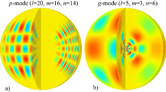
Figure 15: Eigenfunctions (42) of two normal oscillation modes of the Sun: a) p-mode of angular degree $l=20$, angular degree $m=16$, and radial order $n=16$, b) g-mode of $l=5$, $m=3$, and $n=5$. Red and blue-green colors correspond to positive and negative values.

Equations (35) and (37) with boundary conditions (38)-(40) constitute an eigenvalue problem for solar oscillation modes. This eigenvalue problem can be solved numerically for any solar or stellar model. The solution gives the frequencies, $\omega_{nl}$, and the radial eigenfunctions, $\xi_{r}^{(n,l)}(r)$ and ${P^{\prime}}^{(n,l)}(r)$, of the normal modes.

The radial eigenfunctions multiplied by the angular eigenfunctions (22)-(25) represented by the spherical harmonics (29) give three-dimensional oscillation eigenfunctions of the normal modes, e.g.:

$$\xi_{r}(r,\theta,\phi,\omega)=\xi_{r}^{(n,l)}(r)Y_{l}^{m}(\theta,\phi).$$ (42)

Examples of such two eigenfunctions for p- and g-modes are shown in Fig. 15. It illustrates the typical behavior of the modes: the p-modes are concentrated (have the strongest amplitude) in the outer layers of the Sun, and g-modes are mostly confined in the central region.

4.2 JWKB solution

The basic properties of the oscillation modes can be investigated analytically using an asymptotic approximation. In this approximation, we assume that only density $\rho(r)$ varies significantly among the solar properties in the oscillation equations, and seek for an oscillatory solution in the JWKB form:

$$\xi_{r}=A\rho^{-1/2}e^{ik_{r}r},$$ (43)

$$P^{\prime}=B\rho^{1/2}e^{ik_{r}r},$$ (44)

where the radial wavenumber $k_{r}$ is a slowly varying function of $r$; $A$ and $B$ are constants.

Then, substituting these in Eqs (35) and (37) we obtain:

$$\frac{d\xi_{r}}{dr}=-A\rho^{-1/2}\left(-ik_{r}+\frac{1}{H}\right)e^{ik_{r}r},$$ (45)

$$\frac{dP^{\prime}}{dr}=-B\rho^{1/2}\left(-ik_{r}-\frac{1}{H}\right)e^{ik_{r}r},$$ (46)

where

$$H=\left(\frac{d\log\rho}{dr}\right)^{-1},$$ (47)

is the density scale height.

From (45-46) we get a linear system for the constant, $A$, and $B$:

$$\left(-ik_{r}+\frac{1}{H}\right)A-\frac{g}{c^{2}}A+\frac{1}{c^{2}}\left(1-\frac{S_{l}^{2}}{\omega^{2}}\right)B=0,$$ (48)

$$\left(-ik_{r}-\frac{1}{H}\right)B+\frac{g}{c^{2}}B+(N^{2}-\omega^{2})A=0.$$ (49)

It has a non-zero solution when the determinant is equal zero, that is when

$$k_{r}^{2}=\frac{\omega^{2}-\omega_{c}^{2}}{c^{2}}+\frac{S_{l}^{2}}{c^{2}\omega^{2}}\left(N^{2}-\omega^{2}\right),$$ (50)

where

$$\omega_{c}=\frac{c}{2H}$$ (51)

is the acoustic cut-off frequency. Here, we used the relation: $N^{2}=g/H-g^{2}/c^{2}$.

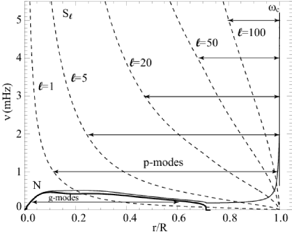
Figure 16: Buoyancy (Brünt-Väisälä) frequency $N$ (thick curve), acoustic cut-off frequency, $\omega_{c}$ (thin curve) and Lamb frequency $S_{l}$ for $l$=1, 5, 20, 50, and 100 (dashed curves) vs. fractional radius $r/R$ for a standard solar model. The horizontal lines with arrows indicate the trapping regions for a g mode with frequency $\nu=0.2$ mHz, and for a sample of five p modes: $l=1$, $\nu=1$ mHz; $l=5$, $\nu=2$ mHz; $l=20$, $\nu=3$ mHz; $l=50$, $\nu=4$ mHz; $l=100$, $\nu=5$ mHz.

The frequencies of solar modes depend on the sound speed, $c$, and three characteristic frequencies: acoustic cut-off frequency, $\omega_{c}$ (51), Lamb frequency, $S_{l}$ (36), and Brünt-Väisälä frequency, $N$ (21). These frequencies calculated for a standard solar model are shown in Fig. 16. The acoustic cut-off and Brünt-Väisälä frequencies depend only on the solar structure, but the Lamb frequency depends also on the mode angular degree, $l$. This diagram is very useful for determining the regions of mode propagation. The waves propagate in the regions where the radial wavenumber is real, that $k_{r}^{2}>0$. If $k_{r}^{2}<0$ then the waves exponentially decay with distance (become ‘evanescent’). The characteristic frequencies define the boundaries of the propagation regions, also called the wave turning points. The region of propagation for p- and g-modes are indicated in Fig. 16, and are discussed in the following sections.

We define a horizontal wavenumber as

$$k_{h}\equiv\frac{L}{r},$$ (52)

where $L=\sqrt{l(l+1)}$. This definition follows from the angular part of the wave equation (27):

$$\frac{1}{r^{2}}\nabla_{h}^{2}Y_{l}^{m}+\frac{l(l+1)}{r^{2}}Y_{l}^{m}=0,$$ (53)

where $\nabla_{h}$ is the horizontal component of gradient. It can be rewritten in terms of a horizontal wavenumber, $k_{h}$, $\frac{1}{r^{2}}\nabla_{h}^{2}Y_{l}^{m}+k_{h}^{2}Y_{l}^{m}=0$ if $k_{h}^{2}=l(l+1)/r^{2}$.

In term of $k_{h}$ the Lamb frequency is $S_{l}=k_{h}c$, and Eq. 50 takes the form:

$$k_{r}^{2}=\frac{\omega^{2}-\omega_{c}^{2}}{c^{2}}+k_{h}^{2}\left(\frac{N^{2}}{\omega^{2}}-1\right),$$ (54)

The frequencies of normal modes are determined for the Borh quantization rule (resonant condition):

$$\int_{r_{1}}^{r_{2}}k_{r}dr=\pi(n+\alpha),$$ (55)

where $r_{1}$ and $r_{2}$ are the radii of the inner and outer turning points where $k_{r}$=0, $n$ is a radial order -integer number, and $\alpha$ is a phase shift which depends on properties of the reflecting boundaries.

4.3 Dispersion relations for p- and g-modes

For high-frequency oscillations, when $\omega^{2}>>N^{2}$, the dispersion relation (50)-(54) can be written as:

$$k_{r}^{2}=\frac{\omega^{2}-\omega_{c}^{2}}{c^{2}}-\frac{S_{l}^{2}}{c^{2}}=\frac{\omega^{2}-\omega_{c}^{2}}{c^{2}}-k_{h}^{2}.$$ (56)

Then, we obtain:

$$\omega^{2}=\omega_{c}^{2}+(k_{r}^{2}+k_{h}^{2})c^{2}\equiv\omega_{c}^{2}+k^{2}c^{2}.$$ (57)

This is a dispersion relation for acoustic (p) modes, $\omega_{c}$ is the acoustic cut-off frequency. The wave with frequencies less than $\omega_{c}$ (or wavelength $\lambda>4\pi H$) do not propagate. These waves exponentially decay, and called ‘evanescent’.

For low-frequency perturbations, when $\omega^{2}<<S_{l}^{2}$, one gets:

$$k_{r}^{2}=\frac{S_{l}^{2}}{c^{2}\omega^{2}}(N^{2}-\omega^{2})=\frac{k_{h}^{2}}{\omega^{2}}(N^{2}-\omega^{2}),$$ (58)

and

$$\omega^{2}=\frac{k_{h}^{2}N^{2}}{k_{r}^{2}}\equiv N^{2}\cos^{2}\theta,$$ (59)

where $\theta$ is the angle between the wavevector, $k$, and horizontal surface.

These waves are called internal gravity waves or g-modes. They propagate mostly horizontally, and only if $\omega^{2}<N^{2}$. The frequency of the internal gravity waves does not depend on the wavenumber, but on the direction of propagation. These waves are evanescent if $\omega^{2}>N^{2}$.

4.4 Frequencies of p- and g-modes

Now, we use the Borh quantization rule (55) and the dispersion relations for the p- and g-modes (57-58) to derive the mode frequencies.

p-modes:

The modes propagate in the region where $k_{r}^{2}>0$; and the radii of the turning points, $r_{1}$ and $r_{2}$, are determined from the relation $k_{r}^{2}=0$:

$$\omega^{2}=\omega_{c}^{2}+\frac{L^{2}c^{2}}{r^{2}}=0.$$ (60)

The acoustic cut-off is only significant near the Sun’s surface. The lower turning point is located in the interior where $\omega_{c}<<\omega$ (Fig. 16. Then, at the lower turning point, $r=r_{1}$: $\omega\approx{Lc}/{r}$, or

$$\frac{c(r_{1})}{r_{1}}=\frac{\omega}{L}$$ (61)

represents the equation for the radius of the lower turning point, $r_{1}$. The upper turning point is determined by the acoustic frequency term: $\omega_{c}(r_{2})\approx\omega$. Since $\omega_{c}(r)$ is a steep function of $r$ near the surface, then

$$r_{2}\approx R.$$ (62)

The p-mode propagation region is illustrated in Fig. 16 Thus, the resonant condition for the p-modes is:

$$\int_{r_{1}}^{R}\sqrt{\frac{\omega^{2}}{c^{2}}-\frac{L^{2}}{r^{2}}}dr=\pi(n+\alpha)$$ (63)

In the case, of the low-degree “global” modes, for which $l<<n$, the lower turning point is almost at the center, $r_{1}\approx 0$, and we obtain Vandakurov1968 :

$$\omega\approx\frac{\pi(n+L/2+\alpha)}{\int_{0}^{R}{dr/c}}.$$ (64)

This relation shows is the spectrum of low-degree p-modes is approximately equidistant with the frequency spacing:

$$\Delta\nu=\left(4\int_{0}^{R}\frac{dr}{c}\right)^{-1}.$$ (65)

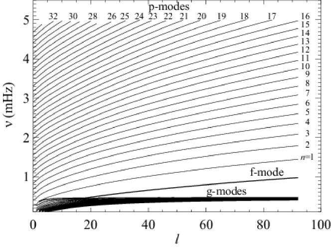
Figure 17: Spectrum of normal modes calculated for a standard solar model. The thick gray curve shows $f$-mode. Labels $p_{1}$-$p_{33}$ mark p-modes of the radial order $n=1,\ldots,33$.

This corresponds very well to the observational power spectrum shown in Fig. 4. According to this relation, the frequencies of mode pairs, $(n,l)$ and $(n-1,l+2)$, coincide. However, calculations to the second-order shows that the frequencies in these pairs are separated by the amount Tassoul1980 ; Gough1993 :

$$\delta\nu_{nl}=\nu_{nl}-\nu_{n-1,l+2}\approx-(4l+6)\frac{\Delta\nu}{4\pi^{2}\nu_{nl}}\int_{0}^{R}\frac{dc}{dr}\frac{dr}{r}.$$ (66)

This is so-called “small separation”. For the Sun, $\Delta\nu\approx 136\mu$Hz, and $\delta\nu\approx 9\mu$Hz. The $l-\nu$ for the p-modes is illustrated in Fig. 17.

g-modes:

The turning points, $k^{r}=0$, are determined from equation (58):

$$N(r)=\omega.$$ (67)

In the propagation region, $k_{r}>0$, (see Fig. 16), far from the turning points ($N>>\omega$):

$$k_{r}\approx\frac{LN}{r\omega}.$$ (68)

Then, from the resonant condition:

$$\int_{r_{1}}^{r_{2}}\frac{L}{\omega}N\frac{dr}{r}=\pi(n+\alpha).$$ (69)

we find an asymptotic formula for the g-mode frequencies:

$$\omega\approx\frac{L\int_{r_{1}}^{r_{2}}N\frac{dr}{r}}{\pi(n+\alpha)}.$$ (70)

It follows that for a given $l$ value the oscillation periods form a regular equally spaced pattern:

$$P=\frac{2\pi}{\omega}=\frac{\pi(n+\alpha)}{L\int_{r_{1}}^{r_{2}}N\frac{dr}{r}}.$$ (71)

The distribution of numerically calculated g-mode periods is shown in Fig. 18.

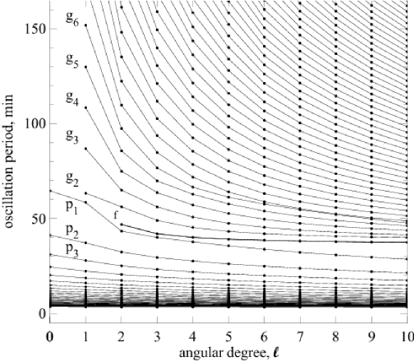
Figure 18: Periods of solar oscillation modes in the angular degree range, $l=0-10$. Labels $g_{1}$-$g_{6}$ mark g-modes of the radial order $n=1,\ldots,6$

4.5 Asymptotic ray-path approximation

The asymptotic approximation provides an important representation of solar oscillations in terms of the ray theory. Consider the wave path equation in the ray approximation:

$$\frac{\partial\vec{r}}{\partial t}=\frac{\partial\omega}{\partial\vec{k}}.$$ (72)

Then, the radial and angular components of this equation are:

$$\frac{dr}{dt}=\frac{\partial\omega}{\partial k_{r}},$$ (73)

$$r\frac{d\theta}{dt}=\frac{\partial\omega}{\partial k_{h}}.$$ (74)

Using the dispersion relation for acoustic (p) modes:

$$\omega^{2}=c^{2}(k_{r}^{2}+k_{h}^{2}),$$ (75)

in which we neglected the $\omega_{c}$ term. (It can be neglected everywhere except near the upper turning point, $R$), we get

$$dt=\frac{dr}{c\left(1-{k_{h}^{2}c^{2}}/{\omega^{2}}\right)^{1/2}}.$$ (76)

Thus, is the travel time from the lower turning point to the surface.

The equation for the acoustic ray path is given by the ratio of equations (74) and (73):

$$r\frac{d\theta}{dr}=\left(\frac{\partial\omega}{\partial k_{h}}\right)/\left(\frac{\partial\omega}{\partial k_{r}}\right)=\frac{k_{h}}{k_{r}},$$ (77)

or

$$r\frac{d\theta}{dr}=\frac{k_{h}}{k_{r}}=\frac{L/r}{\sqrt{{\omega^{2}}/{c^{2}}-{L^{2}}/{r^{2}}}}.$$ (78)

For any given values of $\omega$ and $l$, and initial coordinates, $r$ and $\theta$, this equation gives trajectories of ray paths of p-modes inside the Sun. The ray paths calculated for two solar p-modes are shown in Fig. 19a. They illustrate an important property that the acoustic waves excited by a source near the solar surface travel into the interior and come back to surface. The distance, $\Delta$, between the surface points for one skip can be calculated as the integral:

$$\Delta=2\int_{r_{1}}^{R}d\theta=2\int_{r_{1}}^{R}\frac{L/r}{\sqrt{\omega^{2}/c^{2}-L^{2}/r^{2}}}dr\equiv 2\int_{r_{1}}^{R}\frac{c/r}{\sqrt{\omega^{2}/L^{2}-c^{2}/r^{2}}}dr.$$ (79)

The corresponding travel time is calculated by integrating equation (73):

$$\tau=2\int_{r_{1}}^{R}dt=\int_{r_{1}}^{R}\frac{dr}{c\left(1-{k_{h}^{2}c^{2}}/{\omega^{2}}\right)^{1/2}}\equiv\int_{r_{1}}^{R}\frac{dr}{c\left(1-{L^{2}c^{2}}/{r^{2}\omega^{2}}\right)^{1/2}}.$$ (80)

These equations give a time-distance relation, $\tau-\Delta$, for acoustic waves traveling between two surface points through the solar interior. The ray representation of the solar modes and the time-distance relation provided a motivation for developing time-distance helioseismology (Sec. 7), a local helioseismology method Duvall1993 .

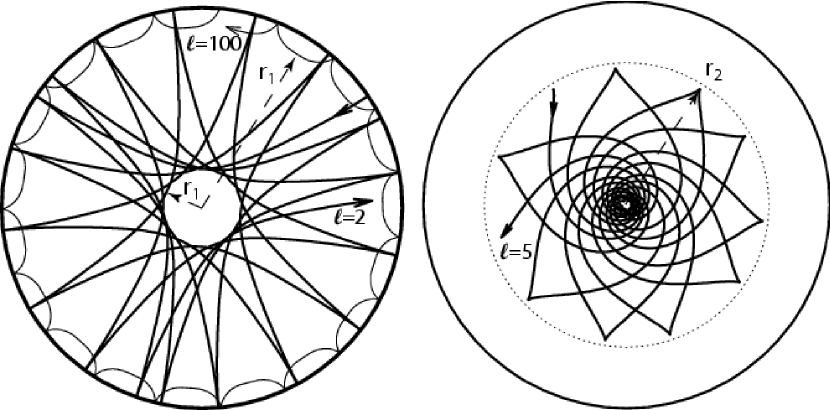
Figure 19: Ray paths for a) two solar p-modes of angular degree $l=2$, frequency $\nu=1429.4\;\mu$Hz (thick curve), and $l=100$, $\nu=3357.5\;\mu$Hz (thin curve); b) g-mode of $l=5$, $\nu=192.6\;\mu$Hz (the dotted curve indicates the base of the convection zone). The lower turning points, $r_{1}$ of the p-modes are shown by arrows. The upper turning points of these modes are close to the surface and not shown. For the g-mode, the upper turning point, $r_{2}$, is shown by arrow. The inner turning point is close to the center and not shown.

The ray paths for g-modes are calculated similarly. For the g-modes, the dispersion relation is:

$$\omega^{2}=\frac{k_{h}^{2}N^{2}}{k_{r}^{2}+k_{h}^{2}}.$$ (81)

Then, the corresponding ray path equation:

$$r\frac{d\theta}{dr}=-\frac{k_{r}}{k_{h}}=-\sqrt{\frac{N^{2}}{\omega^{2}}-1}.$$ (82)

The solution for a g-mode of $l=5,\nu=192.6\mu$Hz is shown in Fig. 19b. Note that the g-mode travels mostly in the central region. Therefore, the frequencies of g-modes are mostly sensitive to the central conditions.

4.6 Duvall’s law

The solar p-modes, observed in the period range of 3–8 minutes, can be considered as high-frequency modes and described by the asymptotic theory quite accurately. Consider the resonant condition (63) for p-modes:

$$\int_{r_{1}}^{R}\left(\frac{\omega^{2}}{c^{2}}-\frac{L^{2}}{r^{2}}\right)^{1/2}dr=\pi(n+\alpha),$$ (83)

Dividing both sides by $\omega$ we get:

$$\int_{r_{1}}^{R}\left(\frac{r^{2}}{c^{2}}-\frac{L^{2}}{\omega^{2}}\right)^{1/2}\frac{dr}{r}=\frac{\pi(n+\alpha)}{\omega}.$$ (84)

Since the lower integral limit, $r_{1}$ depends only on the ratio $L/\omega$, then the whole left-hand side is a function of only one parameter, $L/\omega$, that is:

$$F\left(\frac{L}{\omega}\right)=\frac{\pi(n+\alpha)}{\omega}.$$ (85)

This relation represents so-called Duvall’s law Duvall1982 . It means that a 2D dispersion relation $\omega=\omega(n,l)$ is reduced to the 1D relation between two ratios $L/\omega$ and $(n+\alpha)/\omega$. With an appropriate choice of parameter $\alpha$ (e.g. 1.5) these ratios can easily calculated from a table of observed solar frequencies. An example of such calculations shown in Fig. 20) illustrates that the Duvall’s law holds quite well for the observed solar modes. The short bottom branch that separates from the main curve correspond to f-modes.

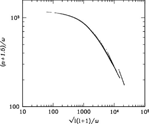
Figure 20: The observed Duvall’s law relation for modes of $l=0-250$.

4.7 Asymptotic sound-speed inversion

The Duvall’s law demonstrate that the asymptotic theory provides a rather accurate description of the observed solar p-modes. Thus, it can be used for solving the inverse problem of helioseismology - determination of the internal properties from the observed frequencies. Theoretically, the internal structure of the Sun is described by the stellar evolution theory Christensen-Dalsgaard1996 . This theory calculates the thermodynamic structure of the Sun during the evolution on the Main Sequence. The evolutionary model of the current age, $\approx 4.6\times 10^{9}$ years, is called the standard solar model. Helioseismology provides estimates of the interior properties, such as the sound-speed profiles, that can be compared with the predictions of the standard model.

Our goal is to find corrections to a solar model from the observed frequency differences between the Sun and the model using the asymptotic formula for the Duvall’s law Christensen-Dalsgaard1988 .

We consider a small perturbation of the sound-speed, $c\rightarrow c+\Delta c$, and the corresponding perturbation of frequency: $\omega\rightarrow\omega+\Delta\omega$. Then, from equation (84) we obtain:

$$\int_{r_{t}}^{R}\left[\frac{(\omega+\Delta\omega)^{2}}{(c+\Delta c)^{2}}-\frac{L^{2}}{r^{2}}\right]^{1/2}dr=\pi(n+\alpha).$$ (86)

Expanding this in terms of $\Delta c/c$ and $\Delta\omega/\omega$ and keeping only the first-order terms we get:

$$\frac{\Delta\omega}{\omega}\int_{r_{t}}^{R}\frac{dr}{c\left(1-{L^{2}c^{2}}/{r^{2}\omega^{2}}\right)^{1/2}}=\int_{r_{t}}^{R}\frac{\Delta c}{c}\frac{dr}{c\left(1-{L^{2}c^{2}}/{r^{2}\omega^{2}}\right)^{1/2}}.$$ (87)

If we introduce a new variable:

$$T=\int_{r_{t}}^{R}\frac{dr}{c\left(1-{L^{2}c^{2}}/{r^{2}\omega^{2}}\right)^{1/2}},$$ (88)

then

$$\frac{\Delta\omega}{\omega}=\frac{1}{T}\int_{r_{t}}^{R}\frac{\Delta c}{c}\frac{dr}{c\left(1-{L^{2}c^{2}}/{r^{2}\omega^{2}}\right)^{1/2}}.$$ (89)

This equation has a simple physical interpretation: $T$ is the travel time of acoustic waves to travel along the acoustic ray path between the lower and upper turning points (Fig. 19). The right-hand side integral is an average of the sound-speed perturbations along this ray path (compare with Eq.(80)).

Equation (89) can be reduced to the Abel integral equation by making a substitution of variables. The new variables are:

$$x=\frac{\omega^{2}}{L^{2}},$$ (90)

$$y=\frac{c^{2}}{r^{2}},$$ (91)

where $x$ is a measured quantity, and $y$ is associated with the sound-speed distribution of an unperturbed solar model.

Then, we obtain an equation for $x$ and $y$:

$$F(x)=\int_{0}^{x}\frac{f(y)dy}{\sqrt{x-y}},$$ (92)

where

$$F(x)=T\frac{\Delta\omega}{\omega}\frac{1}{\sqrt{x}},$$

$$f(y)=\frac{\Delta c}{c}\frac{1}{2y^{3/2}\left(\dfrac{d\log c}{d\log r}+1\right)}.$$

To solve for $f(y)$ we multiply both sides of Eq.(12) by ${dx}/{\sqrt{z-x}}$ and integrate with respect to $x$ from 0 to $z$:

$$\int_{0}^{z}\frac{F(x)dx}{\sqrt{z-x}}=\int_{0}^{z}\frac{dx}{\sqrt{z-x}}\int_{0}^{x}\frac{f(y)dy}{\sqrt{x-y}}=$$

$$=\int_{0}^{x}f(y)dy\int_{y}^{z}\frac{dx}{\sqrt{(z-x)(x-y)}}.$$

Here we changed the order of integration.

Note that

$$\int_{y}^{z}\frac{dx}{\sqrt{(z-x)(x-y)}}=\pi,$$

then

$$\int_{0}^{z}\frac{F(x)dx}{\sqrt{z-x}}=\pi\int_{0}^{x}f(y)dy.$$

Differentiating with respect to $x$, we obtain the final solution:

$$f(y)=\frac{1}{\pi}\frac{d}{dx}\int_{0}^{z}\frac{F(x)dx}{\sqrt{z-x}}.$$ (93)

Then, from $f(y)$ we find the sound-speed correction $\Delta c/c$.

This method based on linearization of the asymptotic Abel integral is called ”differential asymptotic sound-speed inversion” Christensen-Dalsgaard1988 . It provides estimates of the sound-speed deviations from a reference solar model.

Alternatively, the sound-speed profile inside the Sun can be found from a implicit solution of the Abel obtained by differentiating the Duvall’s law equation (84) with respect to variable $y=L/\omega$. Then, this equation can be solved analytically. The solution provides an implicit relationship between the solar radius and sound speed Gough1986 :

$$\ln(r/R)=\int_{r/c}^{R/c_{s}}\frac{dF}{dy}\left(y^{2}-\frac{r^{2}}{c^{2}}\right)^{-1/2}dy,$$ (94)

where $c_{s}$ is the sound speed at the solar surface $r=R$. The calculation of the derivative, $dF/dy$, is essentially differentiation of a smooth function approximating the Duvall’s law, that is differentiating $\pi(n+\alpha)/\omega$ with respect to $L/\omega$. Both of these quantities are obtained from the observed frequency table, $\omega(n,l)$.

The first inversion results using this approach was published by Christensen-Dalsgaard et al Christensen-Dalsgaard1988 . These technique can be generalized by including the Brünt-Väisälä frequency term in the p-mode dispersion relation, and also taking into account the frequency dependence of the phase shift, $\alpha$ Kosovichev1988 . The results show that this inversion procedure provides a good agreement with the solar models, used for testing, except the central core, where the asymptotic and Cowling approximations become inaccurate.

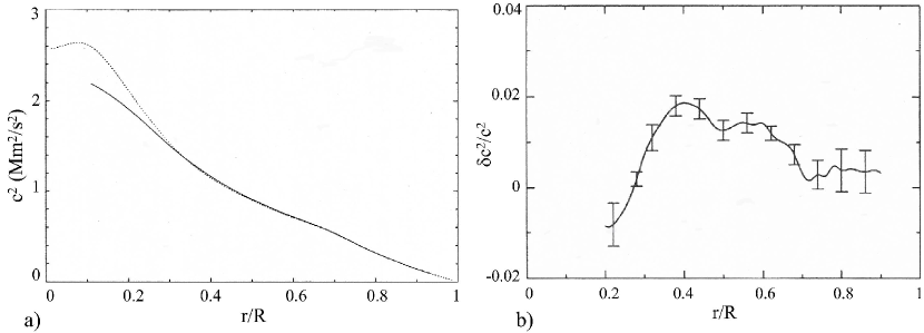
Figure 21: a) Result of the asymptotic sound inversion (solid curve) Kosovichev1988e for the p-mode frequencies Duvall1988 . It confirmed the standard solar model (model 1) Christensen-Dalsgaard1982 (dots). The large discrepancy in the central region is due inaccuracy of the data and the asymptotic approximation. b) The relative difference in the squared sound speed between the asymptotic inversions of the observed and theoretical frequencies.

Figure 21 shows the inversion results Kosovichev1988e for the p-mode frequencies measured by Duvall et al. Duvall1988 . The deviation of the sound speed from a standard solar model is about 1%. Later, the agreement between the solar model and and the helioseismic inversions was improved by using more precise opacity tables and including element diffusion in the model calculations Christensen-Dalsgaard1996 . Also, a more accurate inversion method was developed by using a perturbation theory based on a variational principle for the normal mode frequencies (Sec. 5).

4.8 Surface gravity waves (f-mode)

The surface gravity (f-mode) waves are similar in nature to the surface ocean waves. They are driven by the buoyancy force, and exist because of the sharp density decrease at the solar surface. These waves are missing in the JWKB solution. These waves propagate at the surface boundary where Lagrangian pressure perturbation $\delta P\sim 0$.

To investigate these waves we consider the oscillation equations in terms of $\delta P$ by making use of the relation between Eulerian and Lagrangian variables (10):

$$P^{\prime}=\delta P+g\rho\xi_{r}.$$

The oscillation equations (35) and (37) in terms of $\xi_{r}$ and $\delta P$ are:

$$\frac{d\xi_{r}}{dr}-\frac{L^{2}g}{\omega^{2}r^{2}}\xi_{r}+\left(1-\frac{L^{2}c^{2}}{\omega^{2}r^{2}}\right)\frac{\delta P}{\rho c^{2}}=0,$$ (95)

$$\frac{d\delta P}{dr}+\frac{L^{2}g}{\omega^{2}r^{2}}\delta P-\frac{g\rho f}{r}\xi_{r}=0,$$ (96)

where

$$f\approx\frac{\omega^{2}r}{g}-\frac{L^{2}g}{\omega^{2}r}.$$ (97)

These equations have a peculiar solution:

$$\delta P=0,\;\;f=0.$$

For this solution:

$$\omega^{2}=\frac{Lg}{R}=k_{h}g$$ (98)

-dispersion relation for f-mode.

The eigenfunction equation:

$$\frac{d\xi_{r}}{dr}-\frac{L}{r}\xi_{r}=0$$ (99)

has a solution

$$\xi_{r}\propto e^{k_{h}(r-R)}$$ (100)

exponentially decaying with depth.

These waves are similar in nature to water waves which have the same dispersion relation: $\omega=gk_{h}$. The f-mode waves are incompressible: $\nabla\vec{v}=0.$ These waves are not sensitive to the sound speed but are sensitive to the density gradient at the solar surface. They are used for measurements of the ‘seismic radius’ of the Sun.

4.9 The seismic radius

The frequencies of f-modes:

$$\omega^{2}=gk_{h}\equiv\frac{GM}{R^{2}}\frac{L}{R}\equiv L\frac{GM}{R^{3}}.$$ (101)

If the frequencies are determined in observations for given $l$, then we can define the ‘seismic radius’, $R$, as

$$R=\left(\frac{LGM}{\omega^{2}}\right)^{1/3}.$$ (102)

The procedure of measuring the solar seismic radius is simple Schou1997 . The lower curve in Figure 22a shows the relative difference between the f-mode frequencies of $l=88-250$ calculated for a standard solar model (Model S) and the frequencies obtained from the SOHO/MDI observations. This difference shows that the model frequencies are systematically, by $\approx 6.6\times 10^{-4}$, lower than the observed frequencies. Then from equation (101):

$$\frac{\Delta R}{R}=-\frac{2}{3}\frac{\Delta\nu}{\nu}\approx 4.4\times 10^{-4},$$ (103)

This means that the seismic radius is approximately equal to 695.68 Mm, which is about 0.3 Mm less than the standard radius, 695.99 Mm, used for calibrating the model calculation. This radius is usually measured astrometrically as a position of the inflection point in the solar limb profile. However, in the model calculations it is considered as a height where the optical depth of continuum radiation is equal 1. The difference between this height and the height of the inflection point can explain the discrepancy between the model and seismic radius.

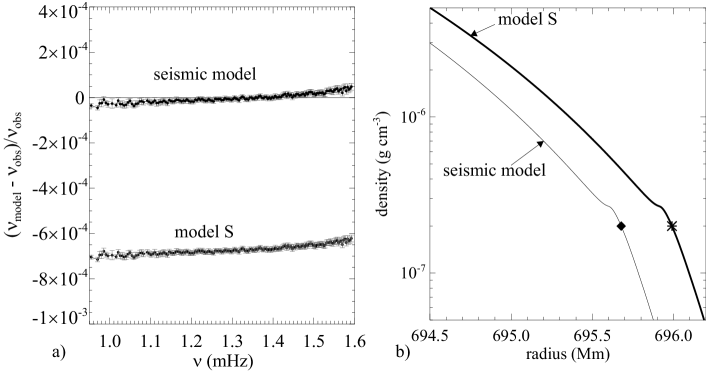
Figure 22: a) Relative differences between the f-mode frequencies of $l=88-250$ computed for a standard solar model (Model S) and the observed frequencies. The ‘seismic model’ frequencies are obtained by scaling the frequencies of model S with factor 1.00066 which corresponds to scaling down the model radius with $(1.00066)^{2/3}\approx 1.00044$. The error bars are $3\sigma$ error estimates of the observed frequencies. b) Density as a function of radius near the surface for the standard and seismic models. The star indicates the photospheric radius. The diamond shows the seismic radius, $695.68$ Mm.

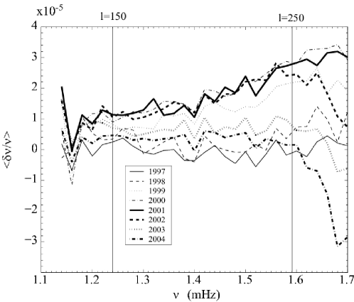
Figure 23: Average relative frequency differences in f-mode $\left\langle\delta\nu/\nu\right\rangle$ as a function of $\left\langle\nu\right\rangle$, average frequencies binned every 20 $\mu$Hz. The reference year is 1996.

Figure 22b illustrates the density profiles in the standard solar model (model S Christensen-Dalsgaard1996 ) and a ‘seismic’ model, calibrated to the seismic radius. The f-mode frequencies of the seismic model match the observations.

Since the f-mode frequencies provide an accurate estimate of the seismic radius, then it is interesting to investigate the variations of the solar radius during the solar activity cycle, which are quite important for understanding physical mechanisms of solar variability (e.g. Rozelot2004 ). Figure 23 shows the f-mode frequency variations during the solar cycle 24, in 1997-2004, relative to the f-mode frequencies observed in 1996 during the solar minimum Lefebvre2005 .

The results show a systematic increase of the f-mode frequency with the increased solar activity, which means a decrease of the seismic radius. However, the variations of the f-mode frequencies are not constant as this is expected from equation (103 for a simple homologous change of the solar structure. A detailed investigation of these variations showed that the frequency dependence can be explained if the variations of the solar structure are not homologous and if the deeper subsurface layers expand but the shallower layers shrink with the increased solar activity Lefebvre2005 ; Lefebvre2007 .

5 General helioseismic inverse problem

In the asymptotic (high-frequency of short-wavelength) approximation (84), the oscillation frequencies depend only on the sound-speed profile. This dependence is expressed in terms of the Abel integral equation (89), which can be solved analytically.

In the general case, the relation between the frequencies and internal properties is more complicated, the frequencies depend not only on the sound speed, but also on other internal properties, and there is no analytical solution. Generally, the frequencies determined from the oscillation equations (35) and (37) depend on the density, $\rho(r)$, the pressure, $P(r)$, and the adiabatic exponent, $\gamma(r)$. However, $\rho$ and $P$ are not independent, and related to each other through the hydrostatic equation:

$$\frac{dP}{dr}=-g\rho,$$ (104)

where $g={Gm}/{r^{2}},\;\;m=4\pi\int_{0}^{r}\rho r^{\prime}\,{}^{2}dr^{\prime}.$ Therefore, only two thermodynamic (hydrostatic) properties of the Sun are independent, e.g. pairs of $(\rho,\gamma)$, $(P,\gamma)$, or their combinations: $(P/\rho,\gamma)$, $(c^{2},\gamma)$, $(c^{2},\rho)$ etc.

The general inverse problem of helioseismology is formulated in terms of small corrections to the standard solar model because the differences between the Sun and the standard model are typically $1\%$ or less. When necessary the corrections can be applied repeatedly, using an iterative procedure.

5.1 Variational principle

We consider the oscillation equations as a formal operator equation in terms of the vector displacement, $\vec{\xi}$:

$$\omega^{2}\vec{\xi}={\cal L}(\vec{\xi}),$$ (105)

where ${\cal L}$ in the general case is an integro-differential operator. If we multiply this equation by $\vec{\xi}^{*}$ and integrate over the mass of the Sun we get:

$$\omega^{2}\int_{V}\rho\vec{\xi}^{*}\cdot\vec{\xi}dV=\int_{V}\vec{\xi}^{*}\cdot{\cal L}\vec{\xi}\rho dV,$$ (106)

where $\rho$ is the model density, $V$ is the solar volume.

Then, the oscillation frequencies can be determined as a ratio of two integrals:

$$\omega^{2}=\frac{\int_{V}\vec{\xi}^{*}\cdot{\cal L}\vec{\xi}\rho dV}{\int_{V}\rho\vec{\xi}^{*}\cdot\vec{\xi}dV}.$$ (107)

The frequencies are expressed in terms of eigenfunctions $\vec{\xi}$ and the solar properties properties represented by coefficients of the operator ${\cal L}$. For small perturbations of solar parameters the frequency change will depend on these perturbations and the corresponding perturbations of the eigenfunctions, e.g.

$$\delta\omega^{2}=\Psi[\delta\rho,\delta\gamma,\delta\vec{\xi}].$$ (108)

The variational principle states that the perturbation of the eigenfunctions constitute second-order corrections, that is to the first-order approximation the frequency variations depend only on variations of the model properties:

$$\delta\omega^{2}\approx\Psi[\delta\rho,\delta\gamma].$$ (109)

The variational principle allows us to neglect the perturbation of the eigenfunctions in the first-order perturbation theory. This was first established by Rayleigh. Thus, equation (107) is called the Rayleigh’s Quotient, and the variational principle is called the Rayleigh’s Principle. The original formulation of this principle is: for an oscillatory system the averaged over period kinetic energy is equal the averaged potential energy. In our case, the left-hand side of equation (106) is proportional to the mean kinetic energy, and the right-hand side is proportional to the potential energy of solar oscillations.

5.2 Perturbation theory

We consider a small perturbation of the operator ${\cal L}$ caused by variations of the solar structure properties:

$${\cal L}(\vec{\xi})={\cal L}_{0}(\vec{\xi})+{\cal L}_{1}(\vec{\xi}).$$

Then, the corresponding frequency perturbations are determined from the following equation:

$$\delta\omega^{2}=\frac{\int_{V}\vec{\xi}^{*}\cdot{\cal L}_{1}\vec{\xi}\rho dV}{\int_{V}\rho\vec{\xi}^{*}\cdot\vec{\xi}dV},$$

or

$$\frac{\delta\omega}{\omega}=\frac{1}{2\omega_{0}I}{\int_{V}\vec{\xi}^{*}\cdot{\cal L}_{1}\vec{\xi}\rho dV},$$ (110)

where

$$I=\int_{V}\rho\vec{\xi}^{*}\cdot\vec{\xi}dV$$ (111)

is so-called mode inertia or mode mass. The mode energy is $E=I\omega_{0}^{2}a^{2}$, where $a$ is the amplitude of the surface displacement. The mode eigenfunctions are usually normalized such that $\xi_{r}(R)=1$.

Using explicit formulations for operator ${\cal L}_{1}$ Eq. 110 can be reduced to a system of integral equations for a chosen pair of independent variables Dziembowski1990 ; Gough1988 ; Gough1990a ; Kosovichev1999 , e.g. for $(\rho,\gamma)$

$$\frac{\delta\omega^{(n,l)}}{\omega^{(n,l)}}=\int_{0}^{R}K_{\rho,\gamma}^{(n,l)}\frac{\delta\rho}{\rho}dr+\int_{0}^{R}K_{\gamma,\rho}^{(n,l)}\frac{\delta\gamma}{\gamma}dr,$$ (112)

where $K_{\rho,\gamma}^{(n,l)}(r)$ and $K_{\gamma,\rho}^{(n,l)}(r)$ are sensitivity (or ‘seismic’) kernels. They are calculated using the initial solar model parameters, $\rho_{0}$, $P_{0}$, $\gamma$, and the oscillation eigenfunctions for these model, $\vec{\xi}$.

5.3 Kernel transformations

The sensitivity kernels for various pairs of solar parameters can be obtained by using the relations among these parameters, which follows from the equations of solar structure (‘stellar evolution theory’).

A general procedure for calculating the sensitivity kernels developed by Kosovichev Kosovichev1999 can be illustrated in an operator form. Consider two pairs of solar variables, $\vec{X}$ and $\vec{Y}$, e.g.

$$\vec{X}=\left(\frac{\delta\rho}{\rho},\frac{\delta\gamma}{\gamma}\right);\;\;\vec{X}=\left(\frac{\delta u}{u},\frac{\delta Y}{Y}\right),$$

where $u=P/\rho$, $Y$ is the helium abundance.

The linearized structure equations (the hydrostatic equilibrium equation and the equation of state) that relates these variables can be written symbolically:

$${\cal A}\vec{X}=\vec{Y}.$$ (113)

Let $\vec{K}_{X}$ and $\vec{K}_{Y}$ be the sensitivity kernels for $X$ and $Y$, then the frequency perturbation is:

$$\frac{\delta\omega}{\omega}=\int_{0}^{R}\vec{K}_{X}\cdot\vec{X}dr\equiv\left<\vec{K}_{X}\cdot\vec{X}\right>,$$ (114)

where $<\cdot>$ denotes the inner product. Similarly,

$$\frac{\delta\omega}{\omega}=\left<\vec{K}_{Y}\cdot\vec{Y}\right>.$$ (115)

Then from equations (114) and (115) we obtain the following relation:

$$\left<\vec{K}_{Y}\cdot\vec{Y}\right>=\left<\vec{K}_{Y}\cdot{\cal A}\vec{X}\right>=\left<{\cal A}^{*}\vec{K}_{Y}\cdot\vec{X}\right>,$$ (116)

where ${\cal A}^{*}$ is an adjoint operator. This operator is adjoint to the stellar structure operator, ${\cal A}$. The second part of equation (116) represent a formal definition of this operator.

From Eq.(114) and (116) we get:

$$\left<{\cal A}^{*}\vec{K}_{Y}\cdot\vec{X}\right>=\left<\vec{K}_{X}\cdot\vec{X}\right>.$$

This equation is valid for any $\vec{X}$ only if

$${\cal A}^{*}\vec{K}_{Y}=\vec{K}_{X}.$$ (117)

That means that the equation for the sensitivity kernels is adjoint to the stellar structure equations. The explicit formulation of the adjoint equations for the sensitivity kernels for various pairs of variables is given in Kosovichev1999 .

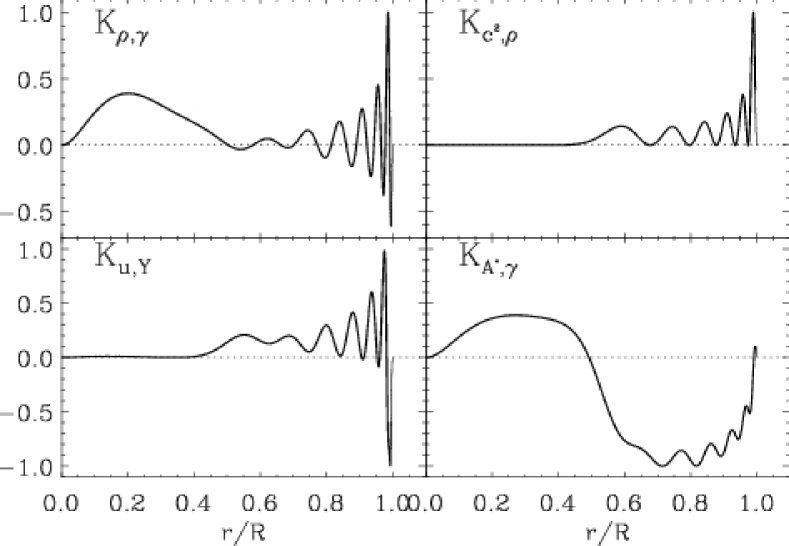
Figure 24: Sensitivity kernels for the acoustic mode of the angular degree, $l$=10, and the radial order, $n$=6. $K_{\rho,\gamma}$ is the kernel for density, $\rho$, at constant adiabatic exponent, $\gamma$; $K_{c^{2},\rho}$ is the kernel for the squared sound speed, $c^{2}$, at constant $\rho$; $K_{u,Y}$ is the kernel for function $u$, - the ratio pressure, $p$, to density at constant helium abundance, $Y$; and $K_{A^{*},\gamma}$ is the kernel for the parameter of convective stability, $A^{*}=rN^{2}/g$, at constant $\gamma$.

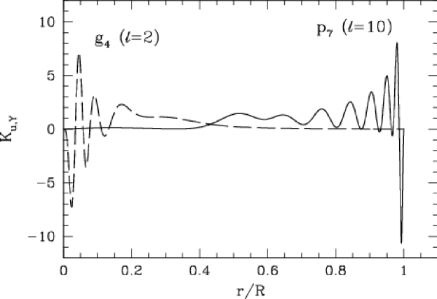
Figure 25: Sensitivity kernels for p- and g-modes for $u=P/\rho$ and helium abundance $Y$.

Examples of the sensitivity kernels for solar properties are shown in Figures 24. Figure 25 illustrates the difference in sensitivities of the p- and g-modes. The frequencies of solar p-modes are mostly sensitive to properties of the outer layers of the Sun while the frequencies of g-modes have the greatest sensitivity to the parameters of the solar core.

5.4 Solution of inverse problem

The variation formulation provides us with a system integral equations (112) for a set of observed mode frequencies. Typically, the number of observed frequencies, $N\simeq 2000$. Thus, we have a problem of determining two functions from this finite set of measurements. In general, it is impossible to determine these functions precisely. We can always find some rapidly oscillating functions, $f(r)$, that being added to the unknowns, $\delta\rho/\rho$ and $\delta\gamma/\gamma$, do not change the values of the integrals, e.g.

$$\int_{0}^{R}K_{\rho,\gamma}^{(n,l)}(r)f(r)dr=0.$$

Such problems without a unique solution are called ”ill-posed”. The general approach is to find a smooth solution that satisfies the integral equations (112) by applying some smoothness constraints to the unknown functions. This is called a regularization procedure.

There are two basic methods for the helioseismic inverse problem:

1. Optimally Localized Averages (OLA) method - (Backus-Gilbert method) Backus1968

2. Regularized Least-Squares (RLS) method - (Tikhonov method) Tikhonov1977

5.5 Optimally localized averages method

The idea of the OLA method is to find a linear combination of data such as the corresponding linear combination of the sensitivity kernels for one unknown has an isolated peak at a given radial point, $r_{0}$, (resembling a $\delta$-function), and the combination for the other unknown is close to zero. Then, this linear combination provides an estimate for the first unknown at $r_{0}$.

Indeed, consider a linear combination of (112) with some unknown coefficient $a^{(n,l)}$:

$$\sum a^{(n,l)}\frac{\delta\omega^{(n,l)}}{\omega^{(n,l)}}==\int_{0}^{R}\sum a^{(n,l)}K_{\rho,\gamma}^{(n,l)}\frac{\delta\rho}{\rho}dr+\int_{0}^{R}\sum a^{(n,l)}K_{\gamma,\rho}^{(n,l)}\frac{\delta\gamma}{\gamma}dr.$$ (118)

If in the first term the linear combination of the kernels is close to a $\delta$-function at $r=r_{0}$, that is

$$\sum a^{(n,l)}K_{\rho,\gamma}^{(n,l)}(r)\simeq\delta(r-r_{0}),$$ (119)

and the linear combination in the second term vanishes:

$$\sum a^{(n,l)}K_{\gamma,\rho}^{(n,l)}(r)\simeq 0,$$ (120)

then equation (118) gives an estimate of the density perturbation, $\delta\rho/\rho$, at $r=r_{0}$:

$$\sum a^{(n,l)}\frac{\delta\omega^{(n,l)}}{\omega^{(n,l)}}\approx\int_{0}^{R}\delta(r-r_{0})\frac{\delta\rho}{\rho}dr=\overline{\left(\frac{\delta\rho}{\rho}\right)}_{r_{0}}.$$ (121)

Of course, the coefficients, $a^{(n,l)}$, of equation (121) must be calculated from conditions (119) and (120) for various target radii $r_{0}$.

The functions,

$$\sum a^{(n,l)}K_{\rho,\gamma}^{(n,l)}(r)\equiv A(r_{0},r),$$ (122)

$$\sum a^{(n,l)}K_{\gamma,\rho}^{(n,l)}(r)\equiv B(r_{0},r),$$ (123)

are called the averaging kernels. They play a fundamental role in the helioseismic inverse theory for determining the resolving power of helioseismic data.

The coefficients, $a^{n,l}$, are determined my minimizing a quadratic form :

$$M(r_{0},A,\alpha,\beta)=\int_{0}^{R}J(r_{0},r)\left[A(r_{0},r)\right]^{2}dr+$$ (124)

$$+\beta\int_{0}^{R}\left[B(r_{0},r)\right]^{2}dr+\alpha\sum_{i,j}E_{n,l;n^{\prime},l^{\prime}}a^{n,l}a^{n^{\prime},l^{\prime}},$$

where function $J(r_{0},r)=12(r-r_{0})^{2}$ provides a localization of the averaging kernels $A(r,r_{0})$ at $r=r_{0}$, $E_{n,l;n^{\prime},l^{\prime}}$ is a covariance matrix of observational errors, $\alpha$ and $\beta$ are regularization parameters. The first integral in eq. (5.5) represents the Backus-Gilbert criterion of $\delta$-ness for $A(r_{0},r)$; the second term minimizes the contribution from $B(r_{0},r)$, thus, effectively eliminating the second unknown function, ($\delta\gamma/\gamma$ in this case); and the last term minimizes the errors. A practical minimization algorithm is presented in Kosovichev1999 . An example of the averaging kernels is shown in Fig. 26

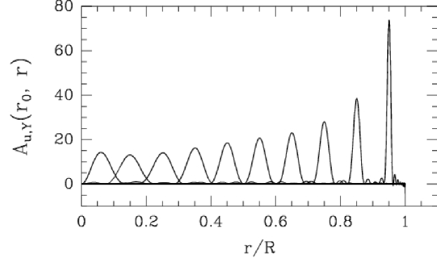
Figure 26: A sample of the optimally localized averaging kernels for the structure function, $u$, the ratio of pressure, $P$, to density, $\rho$, $u=P/\rho$. The second, eliminated, parameter in these kernels is the helium abundance, $Y$.

5.6 Inversion results for solar structure

As an example, consider the results of inversion of the recent data obtained from the MDI instrument on board the SOHO space observatory. The data represent 2176 frequencies of solar oscillations of the angular degree, $l$, from 0 to 250. These frequencies were obtained by fitting peaks in the oscillation power spectra from a 360-day observing run, between May 1, 1996 and April 25, 1997.

Figure 27: The relative frequency difference, scaled with the relative mode inertia factor, $Q=I/I_{0}$ (111), between the Sun and the standard solar model.

Figure 27 shows the relative frequency difference, $\delta\omega/\omega$, between the observed frequencies and the corresponding frequencies calculated for the standard model S Christensen-Dalsgaard1996 . The frequency difference is scaled with a factor $Q\equiv I(\omega)/I_{0}(\omega)$, where $I(\omega)$ is the mode inertia, and $I_{0}(\omega)$ is the mode inertia of radial modes ($l=0$), calculated at the same frequency.

This scaled frequency difference depends mainly on the frequency alone meaning that most of the difference between the Sun and the reference solar model is in the near-surface layers. Physically, this follows from the fact that the p-modes of different $l$ behave similarly near the surface where they propagate almost vertically. This behavior is illustrated by the p-mode ray paths in Fig. 19a, which become almost radial near the surface. In the inversion procedure, this frequency dependence is eliminated by adding an additional “surface term” in equation (112) Kosovichev1999 . However, there is also a significant scatter along the general frequency trend. This scatter is due to the variations of the structure in the deep interior, and it is the basic task of the inversion methods to uncover the variations.

Figure 28: The results of test inversions (points with the error bars, connected with dashed curves) of frequency differences between two solar models for the squared sound speed, $c^{2}$, the adiabatic exponent, $\gamma$, the density, $\rho$, and the parameter of convective stability, $A^{*}$. The solid curves show the actual differences between the two models. Random Gaussian noise was added to the frequencies of a test solar model. The vertical bars show the formal error estimates, the horizontal bars show the characteristic width of the localized averaging kernels. The central points of the averages are plotted at the centers of gravity of the averaging kernels.

First, we test the inversion procedure by considering the frequency difference for two solar models and trying to recover the differences between model properties. Results of the test inversion (Fig. 28) show good agreement with the actual differences. However, the sharp variations, like a peak in the parameter of convective stability, $A^{*}\equiv rN^{2}/g$, at the base of the convection zone, are smoothed. Also, the inner 5% of the Sun and the subsurface layers (outer 2-3%) are not resolved.

Figure 29: The relative differences between the Sun and the standard solar model Christensen-Dalsgaard1996 in the squared sound speed, $c^{2}$, the adiabatic exponent, $\gamma$, the density, $\rho$, and the parameter of convective stability, $A^{*}$, inferred from the solar frequencies determined from the 360-day series of SOHO MDI data.

Then, we apply this procedure to the real solar data. The results (Fig. 29) show that the differences between the inferred structure and the reference solar model (model S) are quite small, generally less than 1%. The small differences provide a justification for the linearization procedure, based on the variational principle. This also means that the modern standard model of the Sun Christensen-Dalsgaard1996 provides an accurate description of the solar properties compared to the earlier solar model Christensen-Dalsgaard1982 , used for the asymptotic inversions (Fig. 21). A significant improvement in the solar modeling was achieved by using more accurate radiative opacity data and by including the effects of gravitational settling of heavy elements and element diffusion. However, recent spectroscopic estimates of the heavy element abundance on the Sun, based on radiative hydrodynamics simulations of solar convection, indicated that the heavy element abundance on the Sun may be lower than the value used in the standard model Asplund2009 . The solar model with a low heavy element abundance do not agree with the helioseismology measurements (e.g. Bahcall2005 ). This problem in the solar modeling has not been resolved. Thus, the helioseismic inferences of the solar structure lead to better understanding of the structure and evolution of the star, and have important applications in other fields of astrophysics.

The prominent peak of the squared sound speed, $\delta c^{2}/c^{2}$, at the base of the convection zone, $r/R\approx 0.7$, indicates on additional mixing which may be caused by rotational shear flows or by convective overshoot. The variation in the sound speed in the energy-generating core at $r/R<0.2$ might be also caused by a partial mixing.

The monotonic decrease of the adiabatic exponent, $\gamma$, in the core was recently explained by the relativistic corrections to the equation of state Elliott1998 . Near surface variations of $\gamma$, in the zones of ionization of helium and hydrogen, and below these zones, are most likely caused by deficiencies in the theoretical models of the weakly coupled plasma employed in the equation of state calculations Dappen2007 .

The monotonic decrease of the squared sound speed variation in the convection zone ($r/R>0.7$) is partly due to an error in the solar seismic radius used to calibrate the standard model Schou1997 , and partly due to the inaccurate description of the subsurface layers by the standard solar model, based on a mixing-length convection theory.

5.7 Regularized least-squares method

The Regularized Least-Squares (RLS) method Tikhonov1977 is based on minimization of the quantity

$${\cal E}\equiv\sum_{n,l}\frac{1}{\sigma^{2}_{n,l}}\left[\frac{\delta\omega^{(n,l)}}{\omega^{(n,l)}}-\int_{0}^{R}\left(K_{(f,g)}^{(n,l)}\frac{\delta f}{f}+K_{(g,f)}^{(n,l)}\frac{\delta g}{g}\right)dr\right]^{2}+$$

$$+\int_{0}^{R}\left[\alpha_{1}\left(L_{1}\frac{\delta f}{f}\right)^{2}+\alpha_{2}\left(L_{2}\frac{\delta g}{g}\right)^{2}\right]dr,$$ (125)

in which the unknown structure correction functions, ${\delta f}/{f}$ and ${\delta g}/{g}$, are both represented by piece-wise linear functions or by cubic splines. The second integral specifies smoothness constraints for the unknown functions, in which $L_{1}$ and $L_{2}$ are linear differential operators, e.g. $L_{1,2}={d^{2}}/{d^{2}r}$; $\sigma_{i}$ are error estimates of the relative frequency differences.

In this inversion method, the estimates of the structure corrections are, once again, linear combinations of the frequency differences obtained from observations, and corresponding averaging kernels exist too. However, unlike the OLA kernels $A(r_{0};r)$, the RLS averaging kernels may have negative sidelobes and significant peaks near the surface, thus making interpretation of the inversion results to some extent ambiguous. Nevertheless, it works well in most cases, and may provide a higher resolution compared to the OLA method.

5.8 Inversions for solar rotation

The eigenfrequencies of a spherically-symmetrical static star are degenerate with respect to the azimuthal number $m$. Rotation breaks the symmetry and splits each mode of radial order, $n$, and angular degree, $l$, into $(2l+1)$ components of $m=-l,...,l$ (mode multiplets). The rotational frequency splitting can be computed using a more general variational principle derived by Lynden-Bell and Ostriker Lynden-Bell1967 . From this variational principle, one can obtain mode frequencies $\omega_{nlm}$ relative to the degenerate frequency $\omega_{nl}$ of the non-rotating star:

$$\Delta\omega_{nlm}\equiv\omega_{nlm}-\omega_{nl}=\frac{1}{I_{nl}}\int_{V}\left[m\mbox{\boldmath$\xi$}\cdot\mbox{\boldmath$\xi$}^{*}+i{\textstyle{\tenbi e}}_{\Omega}(\mbox{\boldmath$\xi$}\times\mbox{\boldmath$\xi$}^{*})\right]\Omega\rho dV,$$ (126)

where ${\textstyle{\tenbi e}}_{\Omega}$ is the unit vector defining the rotation axis, and $\Omega=\Omega(r,\theta)$ is the angular velocity which is a function of radius $r$ and co-latitude $\theta$, and $I_{nl}$ is the mode inertia.

Equation (126) can be rewritten as a two-dimensional integral equation for $\Omega(r,\theta)$:

$$\Delta\omega_{nlm}=\int_{0}^{R}\int_{0}^{\pi}K^{(\Omega)}_{nlm}(r,\theta)\Omega(r,\theta)d\theta dr.$$ (127)

where $K^{(\Omega)}_{nlm}(r,\theta)$ represent the rotational splitting kernels:

$$K^{(\Omega)}_{nlm}(r,\theta)=\frac{m}{I_{nl}}4\pi\rho r^{2}\left\{(\xi_{nl}^{2}-2\xi_{nl}\eta_{nl})(P_{l}^{m})^{2}+\eta_{nl}^{2}\left[\left(\frac{dP_{l}^{m}}{d\theta}\right)^{2}-\right.\right.$$

$$\vspace*{-2cm}\left.\left.-2P_{l}^{m}\frac{dP_{l}^{m}}{d\theta}\frac{\cos\theta}{\sin\theta}+\frac{m^{2}}{\sin^{2}\theta}(P_{l}^{m})^{2}\right]\right\}\sin\theta.$$ (128)

Here $\xi_{nl}$ and $\eta_{nl}$ are the radial and horizontal components of eigenfunctions of the mean spherically symmetric structure of the Sun, $P_{l}^{m}(\theta)$ is an associated normalized Legendre function ($\int_{0}^{\pi}(P_{l}^{m})^{2}\sin\theta d\theta=1$). The kernels are symmetric relative to the equator, $\theta=\pi/2$. Therefore, the frequency splittings are sensitive only to the symmetric component of rotation in the first approximation. The non-symmetric component can, in principle, be determined from the second-order correction to the frequency splitting, or from local helioseismic techniques, such as time-distance seismology.

For a given set of observed frequency splitting, $\Delta\omega_{nlm}$, eq. (126) constitutes a two-dimensional linear inverse problem for the angular velocity, $\Omega(r,\theta)$, which can be solved by the OLA or RLS techniques.

5.9 Results for Solar Rotation

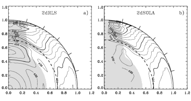
Figure 30: Contour lines of the rotation rate (in nHz) inside the Sun obtained by inverting the rotational frequency splittings from a 144-day observing run from SOHO MDI by the RLS and SOLA methods. The shaded areas are the areas where the localized averaging kernels substantially deviate from the target positions.

As an example, we present the inversion results for solar rotation obtained from SOHO/MDI data. The frequency splitting data were obtained from the 144-day MDI time series by J. Schou for $j=1,...,36$ and $1\leq l\leq 250$ Schou1998 . The total number of measurements in this data set was $M=37366$.

Figure 30 shows results of inversion of the SOI-MDI data by the two methods. The results are generally in good agreement in most of the area where good averaging kernels were obtained. However, the results differ in the high-latitude region. In particular, a prominent feature of the RLS inversion at coordinates (0.2, 0.95) in Fig. 30a, which can be interpreted as a ‘polar jet’, is barely visible in Fig. 30b, showing the OLA inversion of the same data. Therefore, obtaining reliable inversion results in this region and also in the shaded area is one of the main current goals of helioseismology. This can be achieved by obtaining more accurate measurements of rotational frequency splitting and improving inversion techniques. Of course, the radical improvement can be made by observing the polar regions of the Sun. These measurements can be done by using spacecraft with an orbit highly inclined to the ecliptic plane, such as a proposed Solar Polar Imager (SPI) and POLARIS missions Appourchaux2009 .

The most characteristic feature of solar rotation is the differential rotation of the convection zone, which occupies the our 30% of the solar radius. While the radiative core rotates almost uniformly, the equatorial regions of the convection zone rotate significantly faster than the polar regions. The main interest is in understanding the role of Sun’s internal rotation in the dynamo process of generation of solar magnetic fields and the origin of the 11-year sunspot cycle. The results of these measurements (Fig. 31a) reveal two radial shear layers at the bottom of the convection zone (so-called tachocline) and in the upper convective boundary layer. A common assumption is that the solar dynamo operates in the tachocline area (interface dynamo) where it is easier to explain storage of magnetic flux than in the upper convection zone because of the flux buoyancy. However, there are theoretical and observational difficulties with this concept. First, the magnetic field in the tachocline must be quite strong, $\sim 60-160$ kG, to sustain the action of the Coriolis force transporting the emerging flux tubes into high-latitude regions DSilva1993 . The magnetic energy of such field is above the equipartition level of the turbulent energy. Second, the back-reaction such strong field should suppress turbulent motions affecting the Reynolds stresses. Since these turbulent stresses support the differential rotation one should expect significant changes in the rotation rate in the tachocline. However, no significant variations with the 11-year solar cycle are detected. Third, magnetic fields often tend to emerge in compact regions on the solar surface during long periods lasting several solar rotations. This effect is known as ”complexes of activity” or ”active longitudes”. However, the helioseismology observations show that the rotation rate of the solar tachocline is significantly lower than the surface rotation rate. Thus, magnetic flux emerging from the tachocline should be spread over longitudes (with new flux lagging the previously emerged flux) whether it remains connected to the dynamo region or disconnected. It is well-known that sunspots rotate faster than surrounding plasma. This means that the magnetic field of sunspots is anchored in subsurface layers. Observations show that the rotation rate of magnetic flux matches the internal plasma rotation in the upper shear layer (Fig. 31b) indicating that this layer is playing an important role in the solar dynamo, and causing a shift in the dynamo paradigm Brandenburg2005 .

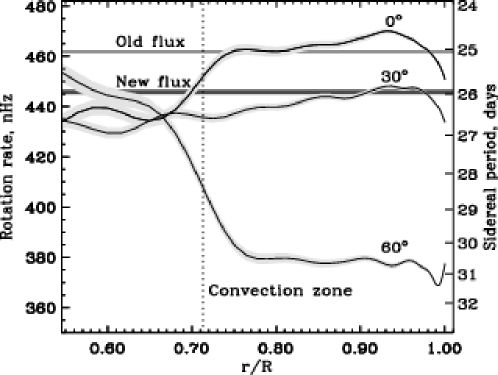
Figure 31: The solar rotation rate as a function of radius at three latitudes. The horizontal lines indicate the rotation rate of the surface magnetic flux at the end of solar cycle 22 (”old magnetic flux”) and at the beginning of cycle 23 (”new magnetic flux”) Benevolenskaya1999

.

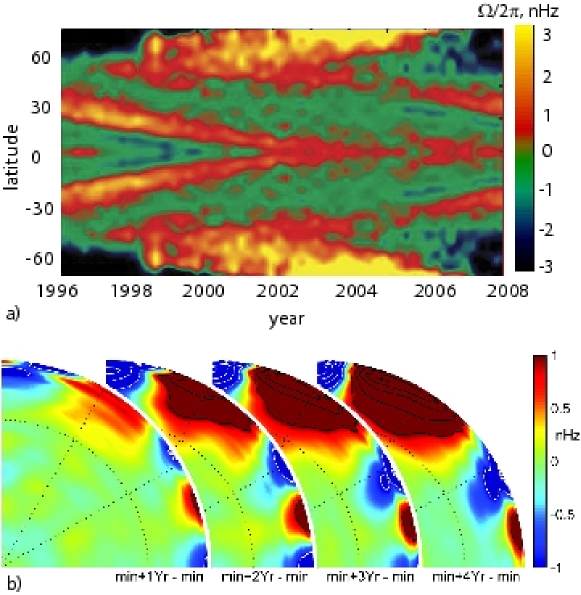
Figure 32: a) Migration of the subsurface zonal flows with latitude during solar cycle 23 from SOHO/MDI data Howe2008 . Red shows zones of faster rotation, green and blue show slower rotation. b) Variations of the zonal flows with depth and latitude during the first 4 years after the solar minimum. Vorontsov2002

Variations in solar rotation clearly related to the 11-year sunspot cycle are observed in the upper convection zone. These are so-called ‘torsional oscillations’ which represent bands of slower and faster rotation, migrating towards the equator as the solar cycle progresses (Fig. 32). The torsional oscillations were first discovered on the Sun’s surface Howard1980 , and then were found in the upper convection zone by helioseismology Kosovichev1997b ; Howe2000 . The depth of these evolving zonal flows is not yet established. However, there are indications that they may be persistent through most of the convection zone, at least, at high latitudes Vorontsov2002 . The physical mechanism is not understood. Nevertheless, it is clear that these zonal flows are closely related to the internal dynamo mechanism that produces toroidal magnetic field. On the solar surface, this field forms sunspots and active regions which tend to appear in the areas of shear flows at the outer (relative to the equator) part of the faster bands. Thus, the torsional flows are an important key to understanding the solar dynamo, and one of the challenges is to establish their precise depth and detect corresponding variations in the thermodynamic structure of the convection zone. Recent modeling of the torsional oscillations by the Lorentz force feedback on differential rotation showed that the poleward-propagating high-latitude branch of the torsional oscillations can be explained as a response of the coupled differential rotation/meridional flow system to periodic forcing in midlatitudes of either mechanical (Lorentz force) or thermal nature Rempel2007 . However, the main equatorward-propagating branches cannot be explained by the Lorenz force, but maybe driven by thermal perturbations caused by magnetic field Spruit2003 . It is intriguing that starting from 2002, during the solar maximum, the helioseismology observations show new branches of ”torsional oscillations” migrating from about $45^{\circ}$ latitude towards the equator (Fig. 32a). They indicate the start of the next solar cycle, number 24, in the interior, and are obviously related to magnetic processes inside the Sun. However, magnetic field of the new cycle appeared on the surface only in 2008.

6 Local-area helioseismology

6.1 Basic principles

In the previous sections we discussed methods of global helioseismology, which are based on inversions of accurately measured frequencies and frequency splitting of normal oscillation modes of the Sun. The frequencies are measured from long time series of observations of the Doppler velocity of the solar disk. These time series are much longer than the mode lifetimes, typically, two or three 36-day-long ‘GONG months’, that is 72 or 108 days. The long time series allow us to resolve individual mode peaks in the power spectrum, and accurately measure the frequencies and other parameters of these modes. However, because of the long integration times global helioseismology cannot capture the fast evolution of magnetic activity in subsurface layers of the Sun. Also, it provides only information about the axisymmetrical structure of the Sun and the differential rotation (zonal flows).

Local helioseismology attempts to determine the subsurface structure and dynamics of the Sun in local areas by analyzing local characteristics of solar oscillations, such as frequency and phase shifts and variations in wave travel times. This is a relatively new and rapidly growing field. It takes advantage of high-resolution observations of solar oscillations, currently available from the GONG+ helioseismology network and the space mission SOHO, and are anticipated from the SDO mission.

6.2 Ring-diagram analysis

Local helioseismology was pioneered by Douglas Gough and Juri Toomre Gough1983 first proposed to measure oscillation frequencies of solar modes as a function of the wavevector, $\omega({\textstyle{\tenbi k}})$, (the dispersion relation) in local areas, and use these measurements for diagnostics of the local flows and thermodynamic properties. They noticed that subsurface variations of temperature cause change in the frequencies, and that subsurface flows result in distortion of the dispersion relation because of the advection effect.

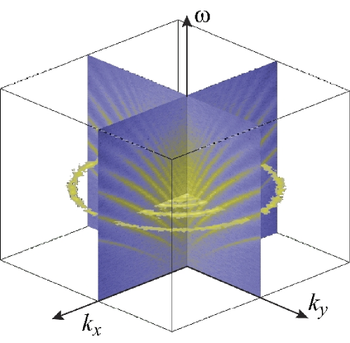
Figure 33: Three-dimensional power spectrum of solar oscillations, $P(k_{x},k_{y},\omega)$. The vertical panels with blue background show the mode ridge structure similar to the global oscillation spectrum shown in Fig. 3. The horizontal cut with transparent background shows the ring structure of the power spectrum at a given frequency (courtesy of Amara Graps).

This idea was implemented by Frank Hill Hill1988 in the form of a ring-diagram analysis. The name of this technique comes from the ring appearance of the 3D dispersion relation, $\omega=\omega(k_{x},k_{y})$, in the $(k_{x},k_{y})$ plane, where $k_{x}$ and $k_{y}$ are $x$- and $y$-components of the wave vector, ${\textstyle{\tenbi k}}$ (Fig. 33). The ridges in the vertical cuts represent the same mode ridges as in Fig. 3, corresponding to the normal oscillation modes of different radial orders $n$.

In the presence of a horizontal flow field, ${\textstyle{\tenbi U}}=(U_{x},U_{y})$ the dispersion relation has the form:

$$\omega=\omega_{0}(k)+{\textstyle{\tenbi k}}\cdot{\textstyle{\tenbi U}}\equiv\omega_{0}+(U_{x}k_{x}+U_{y}k_{y}),$$ (129)

where $\omega_{0}(k)$ is the symmetrical part of the dispersion relation in the $(k_{x},k_{y})$-plane. It depends only on the magnitude of the wave vector, ${\textstyle{\tenbi k}}$. The power spectrum, $P(\omega,{\textstyle{\tenbi k}})$ for each ${\textstyle{\tenbi k}}$ is fitted with a Lorentian profile Haber2002 :

$$P(\omega,{\textstyle{\tenbi k}})=\frac{A}{(\omega-\omega_{0}+k_{x}U_{x}+k_{y}U_{y})^{2}+\Gamma^{2}}+\frac{b_{0}}{k^{3}},$$ (130)

where $A,\omega_{0},\Gamma$, and $b_{0}$ are respectively the amplitude, central frequency, line width and a background noise parameter.

In some realizations, the fitting formula includes the line asymmetry (Sec. 3). Also, the central frequency can be fitted by assuming a power-law relation: $\omega_{0}=ck^{p}$, where $c$ and $p$ are constants Basu2004 ; Hill1988 . This relationship is valid for a polytropic adiabatic stratification, where $p=1/2$ Gough1983 . If the flow velocity changes with depth then the parameter, ${\textstyle{\tenbi U}}$, represent a velocity, averaged with the depth with a weighting factor proportional to the kinetic energy density of the waves, $\rho\mbox{\boldmath$\xi$}\cdot\mbox{\boldmath$\xi$}$ Gough1976 :

$${\textstyle{\tenbi U}}=\frac{\int{\textstyle{\tenbi u}}(z)\rho\mbox{\boldmath$\xi$}\cdot\mbox{\boldmath$\xi$}dz}{\int\rho\mbox{\boldmath$\xi$}\cdot\mbox{\boldmath$\xi$}dz},$$ (131)

where $\mbox{\boldmath$\xi$}(z)=(\xi_{r},\xi_{h})$ is the wave amplitude, given by the mode displacement eigenfunctions (15. The integral is taken over the entire extent of the solar envelope. Equation (131) is solved by the RLS or OLA techniques (Sec. 5).

The ring-diagram method has provided important results about the structure and evolution of large-scale and meridional flows and dynamics of active regions Haber2000 ; Haber2002 ; Haber2004 ; Howe2008 ; Komm2008 . In particular, large-scale patterns of subsurface flows converging around magnetic active regions were discovered Haber2004 . These flows cause variations of the mean meridional circulation with the solar cycle Haber2002 , which may affect transport of magnetic flux of decaying active regions from low latitudes to the polar regions, and thus change the duration and magnitude of the solar cycles Dikpati2006 .

However, the ring-diagram technique in the present formulation has limitations in terms of the spatial and temporal resolution and the depth coverage. The local oscillation power spectra are typically calculated for regions with the horizontal size covering 15 heliographic degrees ($\simeq 180$ Mm). This is significantly larger than the typical size of supergranulation and active regions ($\simeq 30$ Mm). There have been attempts to increase the resolution by doing the measurements in overlapping regions (so-called ”dense-packed diagrams”). However, since such measurements are not independent, their resolution is unclear. The measurements of the power spectra calculated for smaller regions (2-4 degrees in size) increase the spatial resolution but decrease the depth coverage Hindman2006 .

6.3 Time-distance helioseismology (Solar tomography)

Further developments of local seismology led to the idea to perform measurements of local wave distortions in the time-distance space instead of the traditional frequency-wavenumber Fourier space Duvall1993 . In this case, the wave distortions can be measured as perturbations of wave travel times. However, because of the stochastic nature of solar waves it is impossible to track individual wave fronts. Instead, it was suggested to use a cross-covariance (time-distance) function that provides a statistical measure of the wave distortion. Indeed, by cross-correlating solar oscillation signals at two points one may expect that the main contribution to this cross-correlation will be from the waves traveling between these points along the acoustic ray paths Claerbout1968 ; Rickett2000 . Thus, the cross-ccovariance function calculated for oscillation signals measured at two points separated by a distance, $\Delta$, for various time lags, $\tau$, has a peak when the time lag is equal to the travel time of acoustic waves between these points. Physically, the cross-covariance function corresponds to the Green’s function of the wave equation, representing the wave signal from a point source. Of course, in reality, because of the finite wavelength effects, non-uniform distribution of acoustic sources, and complicated wave interaction with turbulence and magnetic fields the interpretation of the travel-time measurements is extremely challenging. Various approximations are used to relate the observed perturbations of the travel times to the internal properties such as sound-speed perturbations and flow velocities. We discuss the basic principles and the current status of the time-distance helioseismology method in Sec. 7.

6.4 Acoustic holography and imaging

The acoustic holography Lindsey1997 and acoustic imaging Chang1997 techniques are developed on the principles of day-light imaging by collecting over large areas on the solar surface coherent acoustic signals emitted from selected target points of the interior. The idea is that the constructed this way signals contain information about objects located below the surface because of wave absorption or scattering at the target points. The phases of individual signals are calculated by using the time-distance relation, $\tau(\Delta)$, f or acoustic waves traveling along the ray paths. The constructed signals, $\psi_{\rm out,in}(t)$, are calculated using the following relation Chou1999 :

$$\psi_{\rm out,in}(t)=\sum_{\tau_{1}}^{\tau_{2}}W\overline{\psi}(\Delta,t\pm\tau),$$ (132)

where $\overline{\psi}(\Delta,t+\tau)$ is the azimuthal-averaged signal at a distance $\Delta$ from a target point at time $t\pm\tau(\Delta)$. The summation variable $\tau$ is equally spaced in the interval $(\tau_{1},\tau_{2})$; and the weighting factor, $W\propto(\sin\Delta/\tau^{2})^{1/2}$, describes the geometrical spreading of acoustic waves with distance. The positive sign in equation (132) corresponds to $\psi_{\rm out}$ constructed with waves traveling outward from a target point (”egression signal” Lindsey1997 ), while the negative sign provides $\psi_{\rm in}$ constructed with the incoming waves (”ingression signal”).

The amplitude and phase of the constructed signals contain information about subsurface perturbation. A practical approach to extract this is to cross-correlate the outgoing and incoming signals Chen1998 ; Braun2000 :

$$C(t)=\int\psi_{\rm in}(t^{\prime})\psi_{\rm out}(t^{\prime}+t)dt^{\prime},$$ (133)

and then to measure time shifts of this function for various target positions relative to the corresponding quiet Sun values. These measurements correspond to the travel-time variations obtained by time-distance helioseismology Chou2000a ; Chou2007 . Further analysis of the travel-time variations is similar to the time-distance helioseismology method Kosovichev1997 . The advantages and disadvantages of the time-distance helioseismology and acoustic holography/imaging are not clear. Both, approaches are being tested using various types of artificial data and applied for measuring subsurface structures and flows. Most of the current inferences of subsurface structures and flows have been obtained using the time-distance approach Duvall1993 ; Kosovichev1997 . The time-distance helioseismology method, also called solar tomography is described in more detail in the following section.

7 Solar tomography

7.1 Time-distance diagram

Solar acoustic waves (p-modes) are excited by turbulent convection near the solar surface and travel through the interior with the speed of sound. Because the sound speed increases with depth the waves are refracted and reappear on the surface at some distance from the source. The wave propagation is illustrated in Figure 34. Waves excited at point A will reappear at the surface points B, C, D, E, F, and others after propagating along the ray paths indicated by the curves connecting these points.

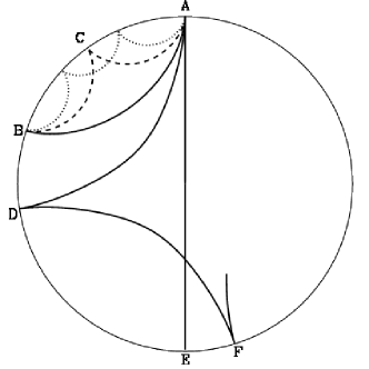
Figure 34: A cross-section diagram through the solar interior showing a sample of wave paths inside the Sun.

The basic idea of time-distance helioseismology, or helioseismic tomography, is to measure the acoustic travel time between different points on the solar surface, and then to use these measurements for inferring variations of wave-speed perturbations and flow velocities in the interior by inversion Duvall1993 . This idea is similar to seismology of Earth. However, unlike in Earth, the solar waves are generated stochastically by numerous acoustic sources in a subsurface layer of turbulent convection.

Therefore, the wave travel time is determined from the cross-covariance function, $\Psi(\tau,\Delta)$, of the oscillation signal, $f(t,{\textstyle{\tenbi r}})$:

$$\Psi(\tau,\Delta)=\int_{0}^{T}f(t,{\textstyle{\tenbi r}}_{1})f^{*}(t+\tau,{\textstyle{\tenbi r}}_{2})dt,$$ (134)

where $\Delta$ is the horizontal distance between two points with coordinates ${\textstyle{\tenbi r}}_{1}$ and ${\textstyle{\tenbi r}}_{2}$, $\tau$ is the lag time, and $T$ is the total time of the observations. The normalized cross-covariance function is called cross-correlation. The time-distance analysis is based on non-normalized cross-covariance. Because of the stochastic nature of solar oscillations, function $\Psi$ must be averaged over some areas to achieve a good signal-to-noise ratio sufficient for measuring the travel times. The oscillation signal, $f(t,{\textstyle{\tenbi r}})$, is measured from the Doppler shift or intensity of a spectral line. A typical cross-covariance function obtained from full-disk solar observations of the Doppler shift shown in Fig. 35a displays a set of ridges. The ridges correspond to acoustic wave packets traveling between two points on the surface directly through the interior or with intermediate reflections (bounces) from the surface as illustrated in Figure 34

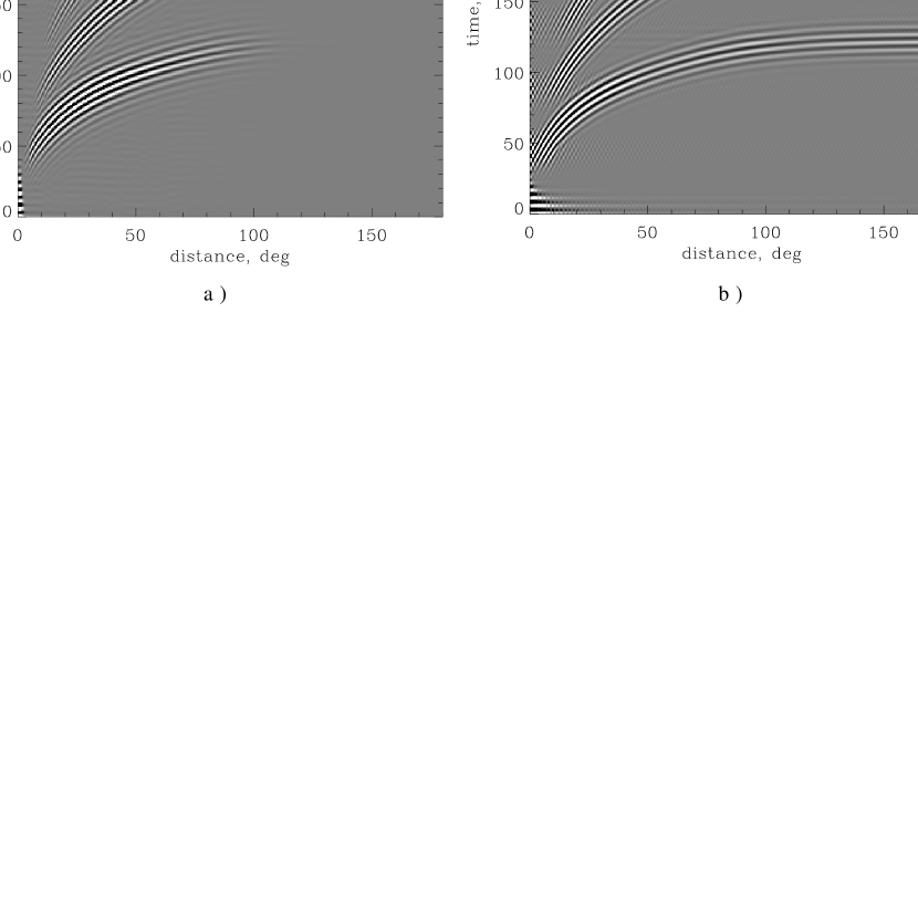
Figure 35: The observational (a) and theoretical (b) cross-covariance functions (time-distance diagrams) as a function of distance on the solar surface, $\Delta$, and the delay time, $\tau$. The lowest set of ridges (‘first bounce’) corresponds to waves propagated to the distance, $\Delta$, without additional reflections from the solar surface. The second from the bottom ridge (‘second bounce’) is produced by the waves arriving to the same distance after one reflection from the surface, and the third ridge (‘third bounce’) results from the waves arriving after two bounces from the surface. The backward ridge at $\tau\approx 250$ min is a continuation of the second-bounce ridge due to the choice of the angular distance range from 0 to 180 degrees (that is, the counterclockwise distance ADF in Fig.34 is substituted with the clockwise distance AF). Because of foreshortening close to the solar limb the observational cross-covariance function covers only $\sim 110$ degrees of distance.

The waves originated at point A may reach point B directly (solid curve) forming the first-bounce ridge, or after one bounce at point C (dashed curve) forming the second-bounce ridge, or after two bounces (dotted curve) - the third-bounce ridge and so on. Because the sound speed is higher in the deeper layers the direct waves arrive first, followed by the second-bounce and higher-bounce waves.

The cross-covariance function represents a time-distance diagram, or a solar ‘seismogram’. Figure 36 shows the cross-covariance signal as a function of time for the travel distance, $\Delta$, of 30 degrees. It consists of three wave packets corresponding to the first, second and third bounces. Ideally, like in Earth seismology, the seismogram can be inverted to infer the structure and flows using a wave theory. However, in practice, modeling the wave fronts is a computationally intensive task. Therefore, the analysis is performed by measuring and inverting the phase and group travel times of the wave packets employing various approximations, the most simple and powerful of which is the ray-path approximation.

Figure 36: The observed cross-covariance signal as a function of time at the distance of 30 degrees.

Generally, the observed solar oscillation signal corresponds to displacement or pressure perturbation, and can be represented in terms of the normal modes eigenfunctions. Therefore, the cross-covariance function also can be expressed in terms of the normal modes. In addition, it can be represented as a superposition of traveling wave packets, as we show in the next subsection Kosovichev1997 . An example of the theoretical cross-covariance function calculated using normal p-modes of the standard solar model is shown in Fig. 35b. This model reproduces the observational cross-covariance function very well in the observed range of distances, from 0 to 90 degrees. The theoretical model was calculated for larger distances than the corresponding observational diagram in Fig. 35a, including points on the far side of the Sun, which is not accessible for measurements. A backward propagating ridge originating from the second-bounce ridge at 180 degrees is a geometrical effect due to the choice of the range of the angular distance from 0 to 180 degrees. In the theoretical diagram (Fig. 35b) one can notice a very weak backward ridge between 30 and 70 degrees and at 120 min. This ridge is due to reflection from the boundary between the convection and radiative zones. However, this signal has not been detected in observations.

7.2 Wave travel times

For simplicity we consider solar oscillation signals observed not far from the disk center and describe these in terms of the radial displacement neglecting the horizontal displacement. The general theory was developed by Nigam and Kosovichev Nigam2010 . In the simple case, the solar oscillation signal can be represented in terms of the radial eigenfunctions (42):

$$f(t,r,\theta,\phi)=\sum_{nlm}a_{nlm}\xi_{r}^{(n,l,m)}(r,\theta,\phi)\exp(i\omega_{nlm}t+i\phi_{nlm}),$$ (135)

where $n,l$ and $m$ are the radial order, angular degree and angular order of a normal mode respectively, $\xi_{nlm}(r,\theta,\phi)$ is a mode eigenfunction in the spherical coordinates, $r,\theta$ and $\phi$, $\omega_{nlm}$ is the eigenfrequency, and $\phi_{nlm}$ is an initial phase of the mode. Using equation (135), we calculate the cross-covariance function, and express it as a superposition of traveling wave packets. Such a representation is important for interpretation of the time-distance data. A similar correspondence between the normal modes and the wave packets has been discussed for surface oscillations in Earth’s seismology Ben-Menahem1964 and also for ocean waves Tindle1974 .

To simplify the analysis, we consider the spherically symmetrical case. In this case, the mode eigenfrequencies do not depend on the azimuthal order $m$. For a radially stratified sphere, the eigenfunctions can be represented in terms of spherical harmonics $Y_{lm}(\theta,\phi)$ (42):

$$\xi_{r}^{(n,l,m)}(r,\theta,\phi)=\xi_{r}^{(n,l)}(r)Y_{lm}(\theta,\phi),$$ (136)

where $\xi_{r}^{(n,l)}(r)$ is the radial eigenfunction Unno1989 .

Using, the convolution theorem Bracewell1986 we express the cross-covariance function in terms of a Fourier intergral:

$$\Psi(\tau,\Delta)=\int_{-\infty}^{\infty}F(\omega,{\textstyle{\tenbi r}}_{1})F^{*}(\omega,{\textstyle{\tenbi r}}_{2})\exp(i\omega\tau)d\omega,$$ (137)

where $F(\omega,{\textstyle{\tenbi r}})$ is Fourier transform of the oscillation signal $f(t,{\textstyle{\tenbi r}})$.

The oscillation signal is considered as band-limited and filtered to select a p-mode frequency range using a Gaussian transfer function:

$$G(\omega)=\exp\left[-\frac{1}{2}\left(\frac{\omega-\omega_{0}}{\delta\omega}\right)^{2}\right],$$ (138)

where $\omega$ is the cyclic frequency, $\omega_{0}$ is the central frequency and $\delta\omega$ is the characteristic bandwidth of the filter. The cross-covariance function in Fig. 1 displays three sets of ridges which correspond to the first, second and third bounces of packets of acoustic wave packets from the surface.

The time series used in our analysis are considerably longer than the travel time $\tau$, therefore, we can neglect the effect of the window function, and represent $F(\omega,{\textstyle{\tenbi r}})$ in the form

$$F(\omega,r,\theta,\phi)\approx A\sum_{nlm}\xi_{r}^{(n,l)}(r)Y_{lm}(\theta,\phi)\delta(\omega-\omega_{nl})\exp\left[-\frac{1}{2}\left(\frac{\omega-\omega_{0}}{\delta\omega}\right)^{2}\right],$$ (139)

where $\delta(x)$ is the delta-function, $\omega_{nl}$ are frequencies of the normal modes, and $A$ is the amplitude of the Gaussian envelope of the amplitude spectrum at $\omega=\omega_{0}$. In addition, we assume the normalization conditions: $\xi_{r}^{(n,l)}(R)=1$, $a_{nl}=A\,G(\omega)$. Then, the cross-covariance function is

$$\Psi(\tau,\Delta)=A^{2}\sum_{nl}\exp\left[-\left(\frac{\omega_{nl}-\omega_{0}}{\delta\omega}\right)^{2}+i\omega_{nl}\tau\right]\sum_{m=-l}^{l}Y_{lm}(\theta_{1},\phi_{1})Y^{*}_{lm}(\theta_{2},\phi_{2}),$$ (140)

where $\theta_{1},\phi_{1}$ and $\theta_{2},\phi_{2}$ are the spherical heliographic coordinates of the two observational points. The sum of the spherical function products

$$\sum_{m=-l}^{l}Y_{lm}(\theta_{1},\phi_{1})Y^{*}_{lm}(\theta_{2},\phi_{2})=\alpha_{l}P_{l}(\cos\Delta),$$ (141)

where $P_{l}(\cos\Delta)$ is the Legendre polynomial, $\Delta$ is the angular distance between points 1 and 2 along the great circle on the sphere, $\cos\Delta=\cos\theta_{1}\cos\theta_{2}+\sin\theta_{1}\sin\theta_{2}\cos(\phi_{2}-\phi_{1})$, and $\alpha_{l}=\sqrt{4\pi/(2l+1)}$. Then, the cross-covariance function is:

$$\Psi(\tau,\Delta)\approx A^{2}\sum_{nl}\alpha_{l}P_{l}(\cos\Delta)\exp\left[-\left(\frac{\omega_{nl}-\omega_{0}}{\delta\omega}\right)^{2}+i\omega_{nl}\tau\right].$$ (142)

For large values of $l\Delta$, but when $\Delta$ is small,

$$P_{l}(\cos\Delta)\simeq\sqrt{\frac{2}{\pi L\Delta}}\cos\left(L\Delta-\frac{\pi}{4}\right).$$ (143)

Thus,

$$\Psi(\tau,\Delta)=A^{2}\sum_{nl}\frac{2}{L\sqrt{\Delta}}\exp\left[-\frac{(\omega_{nl}-\omega_{0})^{2}}{\delta\omega^{2}}\right]\cos(\omega_{nl}\tau)\cos(L\Delta).$$ (144)

Now the double sum can be reduced to a convenient sum of integrals if we regroup the modes so that the outer sum is over the ratio $v=\omega_{nl}/L$ and the inner sum is over $\omega_{nl}$.

According to the ray-path theory, the travel distance $\Delta$ of an acoustic wave is determined by the ratio $v$, which represent the horizontal angular phase velocity ($v=\omega_{nl}/L\equiv(\omega_{nl}/k_{h})/r$). Because of the band-limited nature of the function $G$, only values of $L$ which are close to $L_{0}\equiv\omega_{0}/v$ contribute to the sum. We consider the relation $L$ vs $\omega_{nl}$ as a continuous function along the mode ridges (Fig. 3), and expand $L$ near the central frequency $\omega_{0}$:

$$L\simeq L_{0}+\frac{\partial L}{\partial\omega_{nl}}(\omega_{nl}-\omega_{0})=\frac{\omega_{0}}{v}+\frac{\omega_{nl}-\omega_{0}}{u},$$ (145)

where $u\equiv\partial\omega_{nl}/\partial L$. Furthermore,

$$\cos(\omega_{nl})\tau)\cos(L\Delta)=\cos\left[\left(\tau-\frac{\Delta}{u}\right)\omega_{nl}+\left(\frac{1}{u}-\frac{1}{v}\right)\Delta\omega_{0}\right],$$ (146)

and the other term is identical except that $\tau$ has been replaced with $-\tau$ (negative time lag). The result is that the double sum in equation (146) becomes

$$\Psi(\tau,\Delta)\simeq A^{2}\sum_{v}\frac{2}{L_{0}\sqrt{\Delta}}\sum_{\omega_{nl}}\exp\left[-\frac{(\omega-\omega_{0})^{2}}{\delta\omega^{2}}\right]\cos\left[\left(\pm\tau-\frac{\Delta}{u}\right)+\left(\frac{1}{u}-\frac{1}{v}\right)\Delta\omega_{0}\right].$$ (147)

The inner sum can be approximated by an integral, considering $\omega_{nl}$ as a continuous variable along the mode ridges:

$$\int_{-\infty}^{\infty}d\omega\,\exp\left[-\frac{(\omega-\omega_{0})^{2}}{\delta\omega^{2}}\right]\cos\left[\left(\tau-\frac{\Delta}{u}\right)\omega-\left(\frac{1}{u}-\frac{1}{v}\right)\Delta\omega_{0}\right]=$$ (148)

$$\sqrt{\pi\,\delta\omega^{2}}\exp\left[-\frac{\delta\omega^{2}}{4}\left(\tau-\frac{\Delta}{u}\right)^{2}\right]\cos\left[\omega_{0}\left(\tau-\frac{\Delta}{v}\right)\right].$$

The integration limits reflect the fact that the amplitude function $G(\omega)$ is essentially zero for very large and very small frequencies. Finally, the cross-covariance is expressed in the following form Kosovichev1997 :

$$\Psi(\tau,\Delta)=B\sum_{v}\cos\left[\omega_{0}\left(\tau-\tau_{\rm ph}\right)\right]\exp\left[-\frac{\delta\omega^{2}}{4}\left(\tau-\tau_{\rm gr}\right)^{2}\right],$$ (149)

where $B$ is constant, $\tau_{\rm ph}=\Delta/v$ and $\tau_{\rm gr}=\Delta/u$ are the phase and group travel times. Equation (149) has the form of a Gabor wavelet. The phase and group travel times are measured by fitting individual terms of equation (149) to the observed cross-covariance function using a least-squares technique.

7.3 Deep- and surface-focus measurement schemes

As we have pointed out the travel-time measurements require averaging of the cross-covariance function in order to obtain a good signal-to-noise ratio. Two typical schemes of the spatial averaging suggested by Duvall Duvall1995 are shown in Fig. 37.

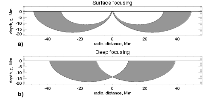
Figure 37: The regions of ray propagation (shaded areas) as a function of depth, $z$, and the radial distance, $\Delta$, from a point on the surface for two observing schemes: ‘surface focusing’ (a) and ‘deep focusing’ (b). The rays are also averaged over a circular regions on the surface, forming three-dimensional figures of revolution.

For the so-called ‘surface-focusing’ scheme (Fig.37a) the measured travel times are mostly sensitive to the near surface condition at the central point where the ray paths are focused. However, by measuring the travel times for several distances and applying an inversion procedure it is possible to infer the distribution of the variations of the wave speed and flow velocities with depth. The averaging also can be done in such a way that the ‘focus’ point is located beneath the surface. An example of the ‘deep-focusing’ scheme is shown in Fig.37b. In this case the travel times are more sensitive to deep structures but still inversions are required for correct interpretation.

7.4 Sensitivity kernels: Ray-path approximation

The travel-time inversion procedures are based on theoretical relations between the travel-time variations and interior properties constituting the forward problem of local helioseismology. Similarly to global helioseismology, these relations are expressed in the form linear integral equations with sensitivity kernels. Two basic types of the sensitivity kernels have been used: ray-path kernels Kosovichev1997 and Born-approximation kernels Birch2000 ; Birch2004 ; Couvidat2006 . The ray-path kernels are based on a simple and generally robust theoretical ray approximation, but they do not take into account finite wavelength effects and thus are not sufficiently accurate for diagnostics of small-scale structures. For reliable inferences it is important to use both these kernels.

In the ray approximation, the travel times are sensitive only to the perturbations along the ray paths given by Hamilton’s equations (72). The variations of the phase travel time obey the Fermat’s Principle:

$$\delta\tau=\frac{1}{\omega}\int_{\Gamma}\delta{\textstyle{\tenbi k}}d{\textstyle{\tenbi r}},$$ (150)

where $\delta{\textstyle{\tenbi k}}$ is the perturbation of the wave vector, ${\textstyle{\tenbi k}}$, due to the structural inhomogeneities and flows along the unperturbed ray path, $\Gamma$. Using the dispersion relation for acoustic waves in the convection zone the travel-time variations can be expressed in terms of the sound-speed, magnetic field strength and flow velocity.

The dispersion relation for magnetoacoustic waves in the convection zone is

$$(\omega-{\textstyle{\tenbi k}}\cdot{\textstyle{\tenbi U}})^{2}=\omega_{c}^{2}+k^{2}c_{f}^{2},$$ (151)

where ${\textstyle{\tenbi U}}$ is the flow velocity, $\omega_{c}$ is the acoustic cut-off frequency, $\;\;c_{f}^{2}=\frac{1}{2}\left(c^{2}+c_{A}^{2}+\sqrt{\left(c^{2}+c_{A}^{2}\right)^{2}-4c^{2}({\textstyle{\tenbi k}}\cdot\mbox{\boldmath$c_{A}$})^{2}/k^{2}}\right)$ is the fast magnetoacoustic speed, $\mbox{\boldmath$c_{A}$}=\mbox{\boldmath$B$}/\sqrt{4\pi\rho}\;\;$ is the vector Alfvén velocity, $B$ is the magnetic field strength, $c$ is the adiabatic sound speed, and $\rho$ is the plasma density. If we assume that, in the unperturbed state ${\textstyle{\tenbi U}}=\mbox{\boldmath$B$}=0$, then, to the first-order approximation

$$\delta\tau=-\int_{\Gamma}\left[\frac{(\mbox{\boldmath$n$}\cdot{\textstyle{\tenbi U}})}{c^{2}}+\frac{\delta c}{c}S+\left(\frac{\delta\omega_{c}}{\omega_{c}}\right)\frac{\omega_{c}^{2}}{\omega^{2}c^{2}S}+\frac{1}{2}\left(\frac{c_{A}^{2}}{c^{2}}-\frac{({\textstyle{\tenbi k}}\cdot\mbox{\boldmath$c_{A}$})^{2}}{k^{2}c^{2}}\right)S\right]ds,\;\;\;$$ (152)

where $n$ is a unit vector tangent to the ray, $S=k/\omega$ is the phase slowness.

Then, we separate the effects of flows and structural perturbations by measuring the travel times of acoustic waves traveling in opposite directions along the same ray path, and calculating the difference, $\tau_{\rm diff}$ and the mean, $\tau_{\rm mean}$, of these reciprocal travel times:

$$\delta\tau_{\rm diff}=-2\int_{\Gamma}\frac{(\mbox{\boldmath$n$}\cdot{\textstyle{\tenbi U}})}{c^{2}}ds;\\$$ (153)

$$\delta\tau_{\rm mean}=-\int_{\Gamma}\left[\frac{\delta c}{c}S+\left(\frac{\delta\omega_{c}}{\omega_{c}}\right)\frac{\omega_{c}^{2}}{\omega^{2}c^{2}S}+\frac{1}{2}\left(\frac{c_{A}^{2}}{c^{2}}-\frac{({\textstyle{\tenbi k}}\cdot\mbox{\boldmath$c_{A}$})^{2}}{k^{2}c^{2}}\right)S\right]ds.$$ (154)

Anisotropy of the last term of equation (154) allows us to separate, at least partly, the magnetic effects from the variations of the sound speed and the acoustic cut-off frequency. The acoustic cut-off frequency, $\omega_{c}$ may be perturbed by surface magnetic fields and by temperature and density inhomogeneities. The effect of the cut-off frequency variation depends strongly on the wave frequency, and, therefore, it results in a frequency dependence in $\tau_{\rm mean}$.

In practice, the travel times are measured for from the cross-covariance functions between selected central points on the solar surface and surrounding quadrants symmetrical relative to the North, South, East and West directions. In each quadrant, the travel times are averaged over narrow ranges of the travel distance, $\Delta$. The travel times of the northward-directed waves are subtracted from the times of the south-directed waves to yield the time, $\tau_{\rm diff}^{\rm NS}$, which is predominantly sensitive to subsurface north-south flows. Similarly, the time differences, $\tau_{\rm diff}^{\rm EW}$, between westward- and eastward directed waves yields a measure of the east-ward flows. The time, $\tau_{\rm diff}^{\rm oi}$, between the outward- and inward-directed waves, averaged over the full annuli, is mainly sensitive to vertical flows and divergence of the horizontal flows. This represents a cross-talk effect between the vertical flows and horizontal flows, which is difficult to resolve when the vertical flows are weak Zhao2003a .

Thus, the effects of flows and structural perturbations are separated from each other by taking the difference and the mean of the reciprocal travel times:

$$\delta\tau_{\rm diff}\approx-2\int_{\Gamma}\frac{(\mbox{\boldmath$n$}{\textstyle{\tenbi U}})}{c^{2}}ds;\\$$ (155)

$$\delta\tau_{\rm mean}\approx-\int_{\Gamma}\frac{\delta w}{c}Sds,$$ (156)

where $c$ is the adiabatic sound speed, $n$ is a unit vector tangent to the ray, $S=k/\omega$ is the phase slowness, $\delta w$ is the local wave speed perturbation:

$$\frac{\delta w}{c}=\frac{\delta c}{c}+\mbox{$\frac{1}{2}$}\left(\frac{c_{A}^{2}}{c^{2}}-\frac{({\textstyle{\tenbi k}}\mbox{\boldmath$c_{A}$})^{2}}{k^{2}c^{2}}\right).$$ (157)

Magnetic field causes anisotropy of the mean travel times, which allows us to separate, in principle, the magnetic effects from the variations of the sound speed (or temperature). So far, only a combined effect of the magnetic fields and temperature variations has been measured reliably.

7.5 Born approximation

The development of a more accurate theory for the travel times, based on the Born approximation is currently under way Birch2000 ; Birch2001 ; Gizon2001 ; Birch2004 ; Couvidat2006 .

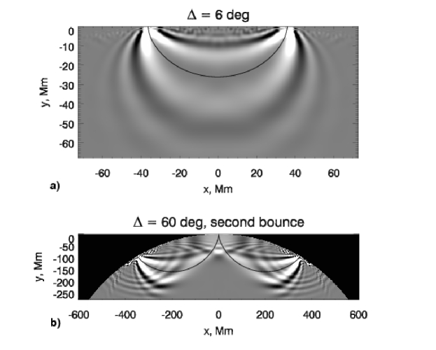
Figure 38: Travel-time sensitivity kernels in the first Born approximation for sound-speed variations as a function of the horizontal, $x$, and vertical, $y$, coordinates for: a) the first-bounce signal for distance $\Delta=6$ degrees, b) the second-bounce signal for $\Delta=60$ degrees. The solid curves show the corresponding ray paths at frequency $\nu=3$ mHz Kosovichev2003 .

One unexpected feature of the single-source travel-time kernels calculated in the Born approximation is that these kernels have zero value along the ray path (called ‘banana-doughnut kernels’). Examples of the Born kernels for the first and the second bounces are shown in Fig.38. The kernels are mostly sensitive to perturbations within the first Fresnel zone.

Figure 39 shows the test results for both the ray and Born approximations for a simple model of a smooth sphere in an uniform medium by comparing with precise numerical results Birch2001 . These results show that for typical perturbations in the solar interior the Born approximation is sufficiently accurate, while the ray approximation significantly overestimates the travel times for perturbations smaller than the size of the first Fresnel zone. That means that the inversion results based on the ray theory may underestimate the strength of the small-scale perturbations. The comparison of the inversion results for sub-surface sound-speed structures beneath sunspots have showed a very good agreement between the ray-paths and Born theories Couvidat2006 .

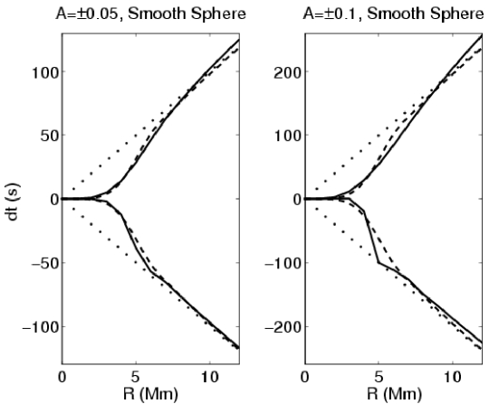
Figure 39: Tests of the ray and Born approximations: travel times for smooth spheres as functions of sphere radius at half maximum. The solid lines are the numerical results. The dashed curves are the Born approximation travel times and the dotted lines are the first order ray approximation. The left panel shows the two perturbations of the relative amplitude, $A=\pm 0.05$. The right panel is for the cases $A=\pm 0.1$. Birch2001

8 Inversion results of solar acoustic tomography

The results of test inversions (e.g. Kosovichev1997 ; Zhao2003a ; Zhao2007 ) demonstrate an accurate reconstruction of sound-speed variations and the horizontal components of subsurface flows. However, vertical flows in deep layers are not resolved because of the predominantly horizontal propagation of the rays in these layers. The vertical velocities are also systematically underestimated in the upper layers. When the vertical flow is weak, e.g. such as in supergranulation, the vertical velocity is not estimated correctly, because the trave-time signal is dominated by the horizontal flow divergence. In such situation, it is difficult to determine even the direction of the vertical flow Zhao2007 . Similarly, the sound-speed variations are underestimated in the deep layers and close to the surface. These limitations of the solar tomography should be taken into account in interpretation of the inversion results.

Here, I briefly present some examples of the local helioseismology inferences obtained by inversion of acoustic travel times.

8.1 Diagnostics of supergranulation.

The data used were for 8.5 hours on 27 January, 1996 from the high resolution mode of the MDI instrument. The results of inversion of these data are shown in Figure 40 Kosovichev1997 . It has been found that, in the upper layers, 2-3 Mm deep, the horizontal flow is organized in supergranular cells, with outflows from the center of the supergranules. The characteristic size of the cells is 20-30 Mm. Comparing with MDI magnetograms, it was found that the cell boundaries coincide with the areas of enhanced magnetic field. These results are consistent with the observations of supergranulation on the solar surface. However, in the layers deeper than $\sim 5$ Mm, the supergranulation pattern disappears. The inversions show an evidence of reverse converging flows at the depth of $\sim 10$ Mm Zhao2003a . This means that supergranulation is a relatively shallow phenomenon.

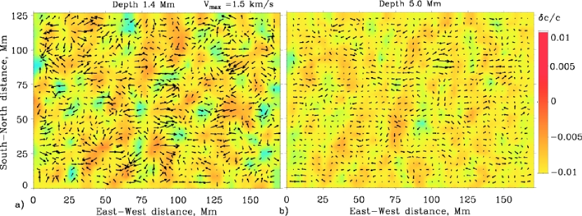
Figure 40: The supergranulation horizontal flow velocity field (arrows) and the sound-speed perturbation (color background) at the depths of 1.4 Mm (a) and 5.0 Mm (b), as inferred from the SOHO/MDI high-resolution data of 27 January 1996. Kosovichev1997

8.2 Structure and dynamics of sunspot

The high-resolution data from the SOHO and Hinode space missions have allowed us to investigate the structure and dynamics beneath sunspots. Figure 41 shows an example of the internal structure of a large sunspot observed on June 17, 1998 Kosovichev2000 . An image of the spot taken in the continuum is shown at the top. The wave-speed perturbations under the sunspot are much stronger than these of the emerging flux, and can reach $\sim 3$ km/s. It is interesting that beneath the spot the perturbation is negative in the subsurface layers and becomes positive in the deeper interior. One can suggest that the negative perturbations beneath the spot are, probably, due to the lower temperature. It follows that magnetic inhibition of convection that makes sunspots cooler is most effective within the top 2-3 Mm of the convection zone. The strong positive perturbation below suggests that the deep sunspot structure is hotter than the surrounding plasma. However, the effects of temperature and magnetic field have not been separated in these inversions. Separating these effects is an important problem of solar tomography. These data also show at a depth of $\sim 4$ Mm connections to the spot of small pores, which have the same magnetic polarity as the main spot. The pores of the opposite polarity are not connected to the main sunspot. This suggests that sunspots represent a tree-like structure in the upper convection zone.

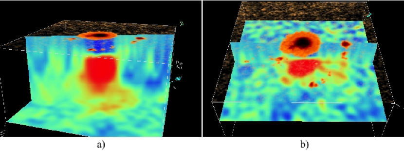
Figure 41: The sound-speed perturbation in a large sunspot observed on June 20, 1998, are shown as vertical and horizontal cuts. The horizontal size of the box is 13 degrees (158 Mm), the depth is 24 Mm. The positive variations of the sound speed are shown in red, and the negative variations (just beneath the sunspot)are in blue. The upper semitransparent panel is the surface intensity image (dark color shows umbra, and light color shows penumbra). In panel b) the horizontal sound-speed plane is located at the depth of 4 Mm, and shows long narrow structures (‘fingers’) connecting the main sunspot structure with surrounding pores the same magnetic polarity as the spot Kosovichev2000 .

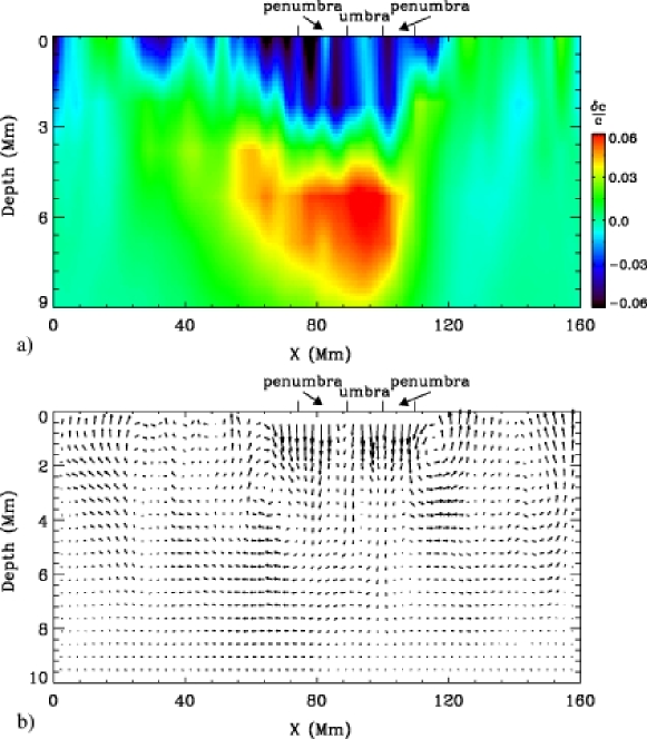
Figure 42: Wave speed perturbation and flow velocities beneath sunspots from Hinode dataZhao2010

Figure 42 shows the subsurface structures and flows beneath a sunspot obtained from Hinode Zhao2010 . A vertical cut along the East-West direction approximately in the middle of a large sunspot observed in AR 10953, May 2, 2007, (Fig. 42a), shows that the wave speed anomalies extend about half of the sunspot size beyond the sunspot penumbra into the plage area. In the vertical direction, the negative wave speed perturbation extends to a depth of 3–4 Mm. The positive perturbation is about 9 Mm deep, but it is not clear whether it extends further, because our inversion cannot reach deeper layers because of the small field of view. Similar two-layer sunspot structures were observed before from SOHO/MDI Kosovichev2000 (Fig. 41). But, it is striking that the new images strongly indicate on the cluster structure of the sunspot Parker1979 . This was not previously seen in the tomographic images of sunspots obtained with lower resolution.

The high-resolution flow field below the sunspot is also significantly more complicated than the previously inferred from SOHO/MDI Zhao2001 , but reveals the same general converging downdraft pattern. A vertical view of an averaged flow field (Fig. 42b) shows nicely the flow structure beneath the active region. Strong downdrafts are seen immediately below the sunspot’s surface, and extends up to 6 Mm in depth. A little beyond the sunspot’s boundary, one can find both upward and inward flows. Clearly, large-scale mass circulations form outside the sunspot, bringing plasma down along the sunspot’s boundary, and back to the photosphere within about twice of the sunspot’s radius. It is remarkable that such an apparent mass circulation is obtained directly from the helioseismic inversions without using any additional constraints, such as forced mass conservation. Previously, the circulation pattern was not that clear.

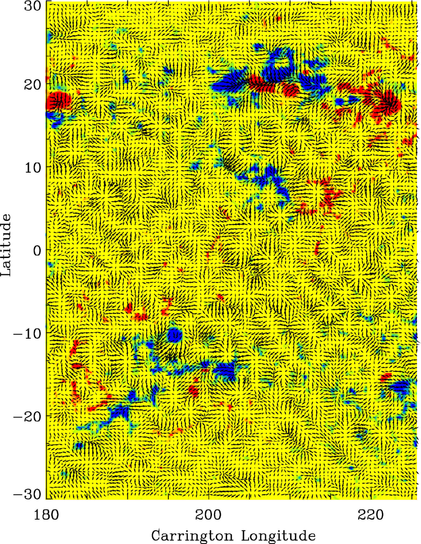
Figure 43: A portion of a synoptic subsurface flow map at depth of 2 Mm. The color background shows the distribution of magnetic field on the surface Zhao2004 .

8.3 Large-scale and meridional flows

Time-distance helioseismology Zhao2004 and also local measurements of the p-mode frequency shifts by the ‘ring-diagram’ analysis Haber2002 ; Haber2000 ; Haber2004 , have provided synoptic maps of subsurface flows over the whole surface of the Sun. Figure 43 shows a portion of a high-resolution synoptic flow map at the depth of 2 Mm below the surface. In addition, to the supergranulation pattern these maps reveal large-scale converging plasma flow around the active regions where magnetic field is concentrated. These flows are particularly well visible in low-resolution synoptic flow maps (Fig. 44). The characteristic speed of these flows is about 50 m/s.

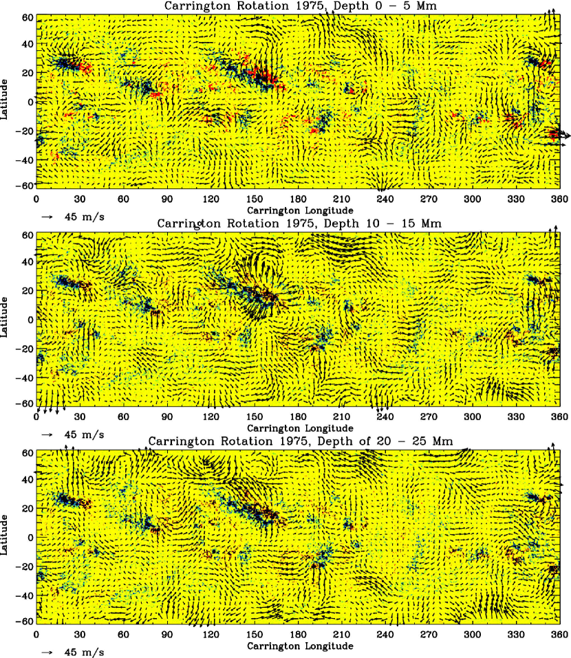
Figure 44: Subsurface synoptic flow maps at three depths. The color background shows the distribution of magnetic field on the surface Zhao2004 .

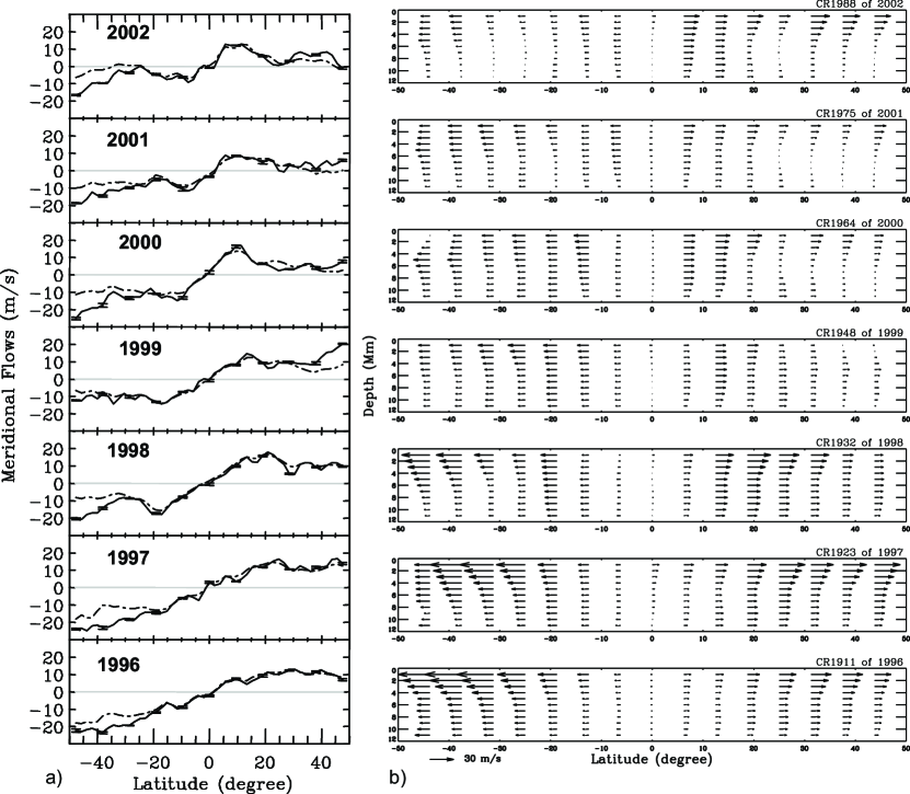
Figure 45: Evolution of subsurface meridional flow during 1996-2002 for various Carrington rotations Zhao2004 .

These stable long-living flow patterns affect the global circulation in the Sun. It is particularly important that these flows change the mean meridional flow from the equator to the poles, slowing it down during the solar maximum years (Fig. 45). This may have important consequences for the solar dynamo theories which invoke the meridional flow to explain the magnetic flux transport into the polar regions and the polar magnetic field polarity reversals usually happening during the period of maximum of solar activity.

9 Conclusion and outlook

During the past decade thanks to the long-term continuous observations from the ground and space the physics of solar oscillations made a tremendous progress in understanding the mechanism of solar oscillations, and in developing new techniques for helioseismic diagnostics of the solar structure and dynamics. However, many problems are still unresolved. Most of them are related to phenomena in strong magnetic field regions and in the deep interior. The prime helioseismology tasks are to detect processes of magnetic field generation and transport in the solar interior, and formation of active regions and sunspots. This will be help to understand the physics of the solar dynamo and the cyclic behavior of solar activity.

For solving these tasks it is very important to continue developing realistic MHD simulations of solar convection and oscillations and to obtain continuous high-resolution helioseismology data for the whole Sun. The recent observations from Hinode have convincingly demonstrated advantages of high-resolution helioseismology, but unfortunately such data are available only for small regions and for short periods of time. A new substantial progress in observations of solar oscillations is expected from the Solar Dynamics Observatory (SDO) space mission launched in February 2010.

The Helioseismic and Magnetic Imager (HMI) instrument on SDO will provide uninterrupted Doppler shift measurements over the whole visible disk of the Sun with a spatial resolution of 0.5 arcsec per pixel ($4096\times 4096$ images) and 40-50 sec time cadence. The total amount of data from this instrument will reach 2 Tb per day. This tremendous amount of data will be processed through a specially developed data analysis pipeline and will provide high-resolution maps of subsurface flows and sound-speed structures Kosovichev2007a . These data will enable investigations of the multi-scale dynamics and magnetism of the Sun and also contribute to our understanding of the Sun as a star.

The tools that will be used in the HMI program include: helioseismology to map and probe the solar convection zone where a magnetic dynamo likely generates this diverse range of activity; measurements of the photospheric magnetic field which results from the internal processes and drives the processes in the atmosphere; and brightness measurements which can reveal the relationship between magnetic and convective processes and solar irradiance variability.

Helioseismology, which uses solar oscillations to probe flows and structures in the solar interior, is providing remarkable new perspectives about the complex interactions between highly turbulent convection, rotation and magnetism. It has revealed a region of intense rotational shear at the base of the convection zone, called the tachocline, which is the likely seat of the global dynamo. Convective flows also have a crucial role in advecting and shearing the magnetic fields, twisting the emerging flux tubes and displacing the photospheric footpoints of magnetic structures present in the corona. Flows of all spatial scales influence the evolution of the magnetic fields, including how the fields generated near the base of the convection zone rise and emerge at the solar surface, and how the magnetic fields already present at the surface are advected and redistributed. Both of these mechanisms contribute to the establishment of magnetic field configurations that may become unstable and lead to eruptions that affect the near-Earth environment.

New methods of local-area helioseismology have begun to reveal the great complexity of rapidly evolving 3-D magnetic structures and flows in the sub-surface shear layer in which the sunspots and active regions are embedded. Most of these new techniques were developed during analysis of MDI observations. As useful as they are, the limitations of MDI telemetry availability and the limited field of view at high resolution has prevented the full exploitation of the methods to answer the important questions about the origins of solar variability. By using these techniques on continuous, full-disk, high-resolution observations, HMI will enable detailed probing of dynamics and magnetism within the near-surface shear layer, and provide sensitive measures of variations in the tachocline.

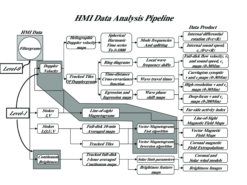
Figure 46: A schematic illustration of the Solar Dynamics Observatory HMI data analysis pipeline and data products. The dark shaded area indicates Level-1 data products. The boxes to the right of this area represent intermediate and final Level-2 data products. The data products are described in detail in the HMI Science Plan Kosovichev2007a .

The scientific operation modes and data products can be divided into four main areas: global helioseismology, local-area helioseismology, line-of-sight and vector magnetography and continuum intensity studies. The principal data flows and products are summarized in Figure 46.

Global Helioseismology:Diagnostics of global changes inside the Sun.

The traditional normal-mode method described in Sec. 4-5, will provide large-scale axisymmetrical distributions of sound speed, density, adiabatic exponent and flow velocities through the whole solar interior from the energy-generating core to the near-surface convective boundary layer. These diagnostics will be based on frequencies and frequency splitting of modes of angular degree up to 1000, obtained for several day intervals each month and up to $l$=300 for each 2-month interval. These will be used to produce a regular sequence of internal rotation and sound-speed inversions to allow observation of the tachocline and average near surface shear.

Local-Area Helioseismology: 3D imaging of the solar interior.

The new methods of local-area helioseismology (Sec. 6-reftomography), time-distance technique, ring-diagram analysis and acoustic holography represent powerful tools for investigating physical processes inside the Sun. These methods on measuring local properties of acoustic and surface gravity waves, such as travel times, frequency and phase shifts. They will provide images of internal structures and flows on various spatial and temporal scales and depth resolution. The targeted high-level regular data products include:

• Full-disk velocity and sound-speed maps of the upper convection zone (covering the top 30 Mm) obtained every 8 hours with the time-distance methods on a Carrington grid;

• Synoptic maps of mass flows and sound-speed perturbations in the upper convection zone for each Carrington rotation with a 2-degree resolution, from averages of full disk time-distance maps;

• Synoptic maps of horizontal flows in upper convection zone for each Carrington rotation with a 5 degree resolution from ring-diagram analyses.

• Higher-resolution maps zoomed on particular active regions, sunspots and other targets, obtained with 4-8-hour resolution for up to 9 days continuously, from the time-distance method;

• Deep-focus maps covering the whole convection zone depth, 0-200 Mm, with 10-15 degree resolution;

• Far-side images of the sound-speed perturbations associated with large active regions every 24 hours.

The HMI science investigation addresses the fundamental problems of solar variability with studies in all interlinked time and space domains, including global scale, active regions, small scale, and coronal connections. One of the prime objectives of the Living With a Star program is to understand how well predictions of evolving space weather variability can be made. The HMI investigation will examine these questions in parallel with the fundamental science questions of how the Sun varies and how that variability drives global change and space weather.

References

- (1) A.S. Eddington, The Internal Constitution of the Stars (1926)
- (2) R.B. Leighton, R.W. Noyes, G.W. Simon, Astrophys. J. 135, 474 (1962)
- (3) P. Mein, Annales d’Astrophysique 29, 153 (1966)
- (4) E.N. Frazier, Astrophys. J. 152, 557 (1968)
- (5) R.K. Ulrich, Astrophys. J. 162, 993 (1970)
- (6) F. Deubner, Astron. Astrophys. 44, 371 (1975)
- (7) E.J. Rhodes, Jr., R.K. Ulrich, G.W. Simon, Astrophys. J. 218, 901 (1977)
- (8) H. Ando, Y. Osaki, Pub. Astron. Soc. Japan 29, 221 (1977)
- (9) J.N. Bahcall, N.A. Bahcall, R.K. Ulrich, Astrophys. J. 156, 559 (1969)
- (10) H.A. Hill, R.T. Stebbins, T.M. Brown, in Bulletin of the American Astronomical Society, Bulletin of the American Astronomical Society, vol. 7 (1975), Bulletin of the American Astronomical Society, vol. 7, p. 478
- (11) A.B. Severny, V.A. Kotov, T.T. Tsap, Nature 259, 87 (1976)
- (12) J.R. Brookes, G.R. Isaak, H.B. van der Raay, Nature 259, 92 (1976)
- (13) P.H. Scherrer, J.M. Wilcox, V.A. Kotov, A.B. Severny, T.T. Tsap, Nature 277, 635 (1979)
- (14) G. Grec, E. Fossat, M. Pomerantz, Nature 288, 541 (1980)
- (15) P.L. Pallé, T. Roca Cortés, B. Gelly, the GOLF Team, in Structure and Dynamics of the Interior of the Sun and Sun-like Stars, ESA Special Publication, vol. 418, ed. by S. Korzennik (1998), ESA Special Publication, vol. 418, pp. 291
- (16) A. Claverie, G.R. Isaak, C.P. McLeod, H.B. van der Raay, T.R. Cortes,
- (17) Y.V. Vandakurov, Soviet Astronomy 11, 630 (1968)
- (18) I. Iben, Jr., J. Mahaffy, Astrophys. J. Lett. 209, L39 (1976)
- (19) J. Christensen-Dalsgaard, D.O. Gough, J.G. Morgan, Astron. Astrophys. 73, 121 (1979)
- (20) J. Christensen-Dalsgaard, D.O. Gough, Astron. Astrophys. 104, 173 (1981)
- (21) T.L. Duvall, Jr., J.W. Harvey, Nature 302, 24 (1983)
- (22) Q.R. Ahmad, et al., Physical Review Letters 89(1), 011301 (2002)
- (23) C.L. Pekeris, Astrophys. J. 88, 189 (1938)
- (24) T.G. Cowling, Mon. Not. Roy. Astron. Soc. 101, 367 (1941)
- (25) P. Ledoux, T. Walraven, Handbuch der Physik 51, 353 (1958)
- (26) D.O. Gough, M.J. Thompson, Mon. Not. Roy. Astron. Soc. 242, 25 (1990)
- (27) W. Dziembowski, P.R. Goode, Memorie della Societa Astronomica Italiana 55, 185 (1984)
- (28) W.A. Dziembowski, P.R. Goode, Astrophys. J. 347, 540 (1989)
- (29) W.A. Dziembowski, P.R. Goode, Astrophys. J. 625, 548 (2005)
- (30) E.J. Rhodes, Jr., R.K. Ulrich, F. Deubner, Astrophys. J. 227, 629 (1979)
- (31) R.K. Ulrich, E.J. Rhodes, Jr., F. Deubner, Astrophys. J. 227, 638 (1979)
- (32) F. Deubner, R.K. Ulrich, E.J. Rhodes, Jr., Astron. Astrophys. 72, 177 (1979)
- (33) T.L. Duvall, Jr., J.W. Harvey, Nature 310, 19 (1984)
- (34) T.L. Duvall, Jr., W.A. Dziembowski, P.R. Goode, D.O. Gough, J.W. Harvey, J.W. Leibacher, Nature 310, 22 (1984)
- (35) T.M. Brown, C.A. Morrow, Astrophys. J. Lett. 314, L21 (1987)
- (36) A.G. Kosovichev, Soviet Astronomy Letters 14, 145 (1988)
- (37) T.M. Brown, J. Christensen-Dalsgaard, W.A. Dziembowski, P. Goode, D.O. Gough, C.A. Morrow, Astrophys. J. 343, 526 (1989)
- (38) R. Rosner, N.O. Weiss, Nature 317, 790 (1985)
- (39) E.N. Parker, Astrophys. J. 408, 707 (1993)
- (40) J.W. Harvey, K. Abdel-Gawad, W. Ball, B. Boxum, F. Bull, J. Cole, L. Cole, S. Colley, K. Dowdney, R. Drake, in Seismology of the Sun and Sun-Like Stars, ESA Special Publication, vol. 286, ed. by E. J. Rolfe (1988), ESA Special Publication, vol. 286, pp. 203–208
- (41) J.R. Brookes, G.R. Isaak, H.B. van der Raay, Mon. Not. Roy. Astron. Soc. 185, 1 (1978)
- (42) G.R. Isaak, C.P. McLeod, P.L. Palle, H.B. van der Raay, T. Roca Cortes, Astron. Astrophys. 208, 297 (1989)
- (43) V. Domingo, B. Fleck, A.I. Poland, Solar Phys. 162, 1 (1995)
- (44) P.H. Scherrer, R.S. Bogart, R.I. Bush, J.T. Hoeksema, A.G. Kosovichev, J. Schou, W. Rosenberg, L. Springer, T.D. Tarbell, A. Title, C.J. Wolfson, I. Zayer, MDI Engineering Team, Solar Phys. 162, 129 (1995)
- (45) J. Leibacher, in IAU Joint Discussion, IAU Joint Discussion, vol. 12 (2003), IAU Joint Discussion, vol. 12
- (46) D.O. Gough, J. Toomre, Solar Phys. 82, 401 (1983)
- (47) F. Hill, Astrophys. J. 333, 996 (1988)
- (48) T.L. Duvall, Jr., S.M. Jefferies, J.W. Harvey, M.A. Pomerantz, Nature 362, 430 (1993)
- (49) A.G. Kosovichev, Astrophys. J. Lett. 469, L61 (1996)
- (50) A.G. Kosovichev, T.L. Duvall, Jr., in SCORe’96 : Solar Convection and Oscillations and their Relationship, Astrophysics and Space Science Library, vol. 225, ed. by F.P. Pijpers, J. Christensen-Dalsgaard, C.S. Rosenthal (1997), Astrophysics and Space Science Library, vol. 225, pp. 241–260
- (51) H. Chang, D. Chou, B. Labonte, The TON Team, Nature 389, 825 (1997)
- (52) C. Lindsey, D.C. Braun, Solar Phys. 192, 261 (2000)
- (53) A.G. Kosovichev, HMI Science Team, Astronomische Nachrichten 328, 339 (2007)
- (54) R.F. Stein, A. Nordlund, Astrophys. J. Lett. 342, L95 (1989)
- (55) J. Zhao, D. Georgobiani, A.G. Kosovichev, D. Benson, R.F. Stein, Å. Nordlund, Astrophys. J. 659, 848 (2007)
- (56) L. Jacoutot, A.G. Kosovichev, A.A. Wray, N.N. Mansour, Astrophys. J. 682, 1386 (2008)
- (57) S.M. Hanasoge, T.L. Duvall, Jr., S. Couvidat, Astrophys. J. 664, 1234 (2007)
- (58) K.V. Parchevsky, J. Zhao, A.G. Kosovichev, Astrophys. J. 678, 1498 (2008)
- (59) T. Hartlep, J. Zhao, N.N. Mansour, A.G. Kosovichev, Astrophys. J. 689, 1373 (2008)
- (60) T.R. Rimmele, P.R. Goode, E. Harold, R.T. Stebbins, Astrophys. J. Lett. 444, L119 (1995)
- (61) R. Skartlien, M.P. Rast, Astrophys. J. 535, 464 (2000)
- (62) R.F. Stein, Å. Nordlund, Astrophys. J. 546, 585 (2001)
- (63) M. Germano, U. Piomelli, P. Moin, W.H. Cabot, Physics of Fluids 3, 1760 (1991)
- (64) P. Moin, K. Squires, W. Cabot, S. Lee, Physics of Fluids 3, 2746 (1991)
- (65) F. Baudin, R. Samadi, M. Goupil, T. Appourchaux, C. Barban, P. Boumier, W.J. Chaplin, P. Gouttebroze, Astron. Astrophys. 433, 349 (2005)
- (66) L. Jacoutot, A.G. Kosovichev, A. Wray, N.N. Mansour, Astrophys. J. Lett. 684, L51 (2008)
- (67) T.L. Duvall, Jr., S.M. Jefferies, J.W. Harvey, Y. Osaki, M.A. Pomerantz, Astrophys. J. 410, 829 (1993)
- (68) T. Toutain, T. Appourchaux, C. Fröhlich, A.G. Kosovichev, R. Nigam, P.H. Scherrer, Astrophys. J. Lett. 506, L147 (1998)
- (69) M. Gabriel, Astron. Astrophys. 265, 771 (1992)
- (70) R. Nigam, A.G. Kosovichev, P.H. Scherrer, J. Schou, Astrophys. J. Lett. 495, L115+ (1998)
- (71) U. Mitra-Kraev, A.G. Kosovichev, T. Sekii, Astron. Astrophys. 481, L1 (2008)
- (72) I.W. Roxburgh, S.V. Vorontsov, Mon. Not. Roy. Astron. Soc. 292, L33 (1997)
- (73) G. Severino, M. Magrì, M. Oliviero, T. Straus, S.M. Jefferies, Astrophys. J. 561, 444 (2001)
- (74) R. Wachter, A.G. Kosovichev, Astrophys. J. 627, 550 (2005)
- (75) D. Georgobiani, R.F. Stein, Å. Nordlund, Astrophys. J. 596, 698 (2003)
- (76) T. Kosugi, K. Matsuzaki, T. Sakao, T. Shimizu, Y. Sone, S. Tachikawa, T. Hashimoto, K. Minesugi, A. Ohnishi, T. Yamada, S. Tsuneta, H. Hara, K. Ichimoto, Y. Suematsu, M. Shimojo, T. Watanabe, S. Shimada, J.M. Davis, L.D. Hill, J.K. Owens, A.M. Title, J.L. Culhane, L.K. Harra, G.A. Doschek, L. Golub, Solar Phys. 243, 3 (2007)
- (77) S. Tsuneta, K. Ichimoto, Y. Katsukawa, S. Nagata, M. Otsubo, T. Shimizu, Y. Suematsu, M. Nakagiri, M. Noguchi, T. Tarbell, A. Title, R. Shine, W. Rosenberg, C. Hoffmann, B. Jurcevich, G. Kushner, M. Levay, B. Lites, D. Elmore, T. Matsushita, N. Kawaguchi, H. Saito, I. Mikami, L.D. Hill, J.K. Owens, Solar Phys. 249, 167 (2008)
- (78) R. Nigam, A.G. Kosovichev, Astrophys. J. Lett. 505, L51+ (1998)
- (79) T.L. Duvall, Jr., A.G. Kosovichev, K. Murawski, Astrophys. J. Lett. 505, L55+ (1998)
- (80) K. Murawski, T.L. Duvall, Jr., A.G. Kosovichev, in Structure and Dynamics of the Interior of the Sun and Sun-like Stars, ESA Special Publication, vol. 418, ed. by S. Korzennik (1998), ESA Special Publication, vol. 418, pp. 825
- (81) D.C. Braun, T.L. Duvall, Jr., B.J. Labonte, Astrophys. J. Lett. 319, L27 (1987)
- (82) P.S. Cally, Mon. Not. Roy. Astron. Soc. 395, 1309 (2009)
- (83) K.V. Parchevsky, A.G. Kosovichev, Astrophys. J. Lett. 666, L53 (2007)
- (84) K. Parchevsky, A. Kosovichev, E. Khomenko, V. Olshevsky, M. Collados, ArXiv e-prints (2010)
- (85) K. Nagashima, T. Sekii, A.G. Kosovichev, H. Shibahashi, S. Tsuneta, K. Ichimoto, Y. Katsukawa, B. Lites, S. Nagata, T. Shimizu, R.A. Shine, Y. Suematsu, T.D. Tarbell, A.M. Title, Pub. Astron. Soc. Japan 59, 631 (2007)
- (86) M. Schüssler, A. Vögler, Astrophys. J. Lett. 641, L73 (2006)
- (87) D.C. Braun, C. Lindsey, Y. Fan, S.M. Jefferies, Astrophys. J. 392, 739 (1992)
- (88) S.M. Hanasoge, Astrophys. J. 680, 1457 (2008)
- (89) E. Khomenko, M. Collados, Astron. Astrophys. 506, L5 (2009)
- (90) A.G. Kosovichev, V.V. Zharkova, Nature 393, 317 (1998)
- (91) A.G. Kosovichev, in Solar MHD Theory and Observations: A High Spatial Resolution Perspective, Astronomical Society of the Pacific Conference Series, vol. 354, ed. by J. Leibacher, R. F. Stein, & H. Uitenbroek (2006), Astronomical Society of the Pacific Conference Series, vol. 354, pp. 154
- (92) A.G. Kosovichev, in Proceedings of SOHO 18/GONG 2006/HELAS I, Beyond the spherical Sun, ESA Special Publication, vol. 624 (2006), ESA Special Publication, vol. 624
- (93) A.G. Kosovichev, Solar Phys. 238, 1 (2006)
- (94) A. Donea, D.C. Braun, C. Lindsey, Astrophys. J. Lett. 513, L143 (1999)
- (95) A. Donea, C. Lindsey, Astrophys. J. 630, 1168 (2005)
- (96) A. Donea, D. Besliu-Ionescu, P.S. Cally, C. Lindsey, V.V. Zharkova, Solar Phys. 239, 113 (2006)
- (97) A.G. Kosovichev, Astrophys. J. Lett. 670, L65 (2007)
- (98) M. Tassoul, Astrophys. J. Suppl. 43, 469 (1980)
- (99) D.O. Gough, in Astrophysical Fluid Dynamics - Les Houches 1987 (1993), pp. 399–560
- (100) T.L. Duvall, Jr., Nature 300, 242 (1982)
- (101) J. Christensen-Dalsgaard, W. Dappen, S.V. Ajukov, E.R. Anderson, H.M. Antia, S. Basu, V.A. Baturin, G. Berthomieu, B. Chaboyer, S.M. Chitre, A.N. Cox, P. Demarque, J. Donatowicz, W.A. Dziembowski, M. Gabriel, D.O. Gough, D.B. Guenther, J.A. Guzik, J.W. Harvey, F. Hill, G. Houdek, C.A. Iglesias, A.G. Kosovichev, J.W. Leibacher, P. Morel, C.R. Proffitt, J. Provost, J. Reiter, E.J. Rhodes, Jr., F.J. Rogers, I.W. Roxburgh, M.J. Thompson, R.K. Ulrich, Science 272, 1286 (1996)
- (102) J. Christensen-Dalsgaard, D.O. Gough, M.J. Thompson, in Seismology of the Sun and Sun-Like Stars, ESA Special Publication, vol. 286, ed. by E. J. Rolfe (1988), ESA Special Publication, vol. 286, pp. 493–497
- (103) D.O. Gough, in NATO ASIC Proc. 169: Seismology of the Sun and the Distant Stars, ed. by D. O. Gough (1986), pp. 125–140
- (104) A.G. Kosovichev, K.V. Parchevskii, Soviet Astronomy Letters 14, 201 (1988)
- (105) T.L. Duvall, Jr., J.W. Harvey, K.G. Libbrecht, B.D. Popp, M.A. Pomerantz, Astrophys. J. 324, 1158 (1988)
- (106) J. Christensen-Dalsgaard, Mon. Not. Roy. Astron. Soc. 199, 735 (1982)
- (107) J. Schou, A.G. Kosovichev, P.R. Goode, W.A. Dziembowski, Astrophys. J. Lett. 489, L197+ (1997)
- (108) J.P. Rozelot, S. Lefebvre, S. Pireaux, A. Ajabshirizadeh, Solar Phys. 224, 229 (2004)
- (109) S. Lefebvre, A.G. Kosovichev, Astrophys. J. Lett. 633, L149 (2005)
- (110) S. Lefebvre, A.G. Kosovichev, J.P. Rozelot, Astrophys. J. Lett. 658, L135 (2007)
- (111) W.A. Dziembowski, A.A. Pamyatnykh, R. Sienkiewicz, Mon. Not. Roy. Astron. Soc. 244, 542 (1990)
- (112) D.O. Gough, A.G. Kosovichev, in Seismology of the Sun and Sun-Like Stars, ESA Special Publication, vol. 286, ed. by E. J. Rolfe (1988), ESA Special Publication, vol. 286, pp. 195–201
- (113) D.O. Gough, A.G. Kosovichev, in IAU Colloq. 121: Inside the Sun, Astrophysics and Space Science Library, vol. 159, ed. by G. Berthomieu & M. Cribier (1990), Astrophysics and Space Science Library, vol. 159, pp. 327
- (114) A.G. Kosovichev, Journal of Computational and Applied Mathematics 109, 1 (1999)
- (115) G.E. Backus, J.F. Gilbert, Geophysical Journal 16, 169 (1968)
- (116) V.Y. Tikhonov, A. N.; Arsenin, Solution of Ill-posed Problems (Washington: Winston & Sons, 1977)
- (117) M. Asplund, N. Grevesse, A.J. Sauval, P. Scott, Ann. Rev. Astron. Astrophys. 47, 481 (2009)
- (118) J.N. Bahcall, A.M. Serenelli, S. Basu, Astrophys. J. Lett. 621, L85 (2005)
- (119) J.R. Elliott, A.G. Kosovichev, Astrophys. J. Lett. 500, L199+ (1998)
- (120) W. Däppen, in Solar and Stellar Physics Through Eclipses, Astronomical Society of the Pacific Conference Series, vol. 370, ed. by O. Demircan, S. O. Selam, & B. Albayrak (2007), Astronomical Society of the Pacific Conference Series, vol. 370, pp. 3
- (121) D. Lynden-Bell, J.P. Ostriker, Mon. Not. Roy. Astron. Soc. 136, 293 (1967)
- (122) J. Schou, H.M. Antia, S. Basu, R.S. Bogart, R.I. Bush, S.M. Chitre, J. Christensen-Dalsgaard, M.P. di Mauro, W.A. Dziembowski, A. Eff-Darwich, D.O. Gough, D.A. Haber, J.T. Hoeksema, R. Howe, S.G. Korzennik, A.G. Kosovichev, R.M. Larsen, F.P. Pijpers, P.H. Scherrer, T. Sekii, T.D. Tarbell, A.M. Title, M.J. Thompson, J. Toomre, Astrophys. J. 505, 390 (1998)
- (123) T. Appourchaux, P. Liewer, M. Watt, D. Alexander, V. Andretta, F. Auchère, P. D’Arrigo, J. Ayon, T. Corbard, S. Fineschi, W. Finsterle, L. Floyd, G. Garbe, L. Gizon, D. Hassler, L. Harra, A. Kosovichev, J. Leibacher, M. Leipold, N. Murphy, M. Maksimovic, V. Martinez-Pillet, B.S.A. Matthews, R. Mewaldt, D. Moses, J. Newmark, S. Régnier, W. Schmutz, D. Socker, D. Spadaro, M. Stuttard, C. Trosseille, R. Ulrich, M. Velli, A. Vourlidas, C.R. Wimmer-Schweingruber, T. Zurbuchen, Experimental Astronomy 23, 1079 (2009)
- (124) S. D’Silva, R.F. Howard, Solar Phys. 148, 1 (1993)
- (125) A. Brandenburg, Astrophys. J. 625, 539 (2005)
- (126) E.E. Benevolenskaya, J.T. Hoeksema, A.G. Kosovichev, P.H. Scherrer, Astrophys. J. Lett. 517, L163 (1999)
- (127) R. Howe, Advances in Space Research 41, 846 (2008)
- (128) S.V. Vorontsov, J. Christensen-Dalsgaard, J. Schou, V.N. Strakhov, M.J. Thompson, Science 296, 101 (2002)
- (129) R. Howard, B.J. Labonte, Astrophys. J. Lett. 239, L33 (1980)
- (130) A.G. Kosovichev, J. Schou, Astrophys. J. Lett. 482, L207+ (1997)
- (131) R. Howe, J. Christensen-Dalsgaard, F. Hill, R.W. Komm, R.M. Larsen, J. Schou, M.J. Thompson, J. Toomre, Science 287, 2456 (2000)
- (132) M. Rempel, Astrophys. J. 655, 651 (2007)
- (133) H.C. Spruit, Solar Phys. 213, 1 (2003)
- (134) D.A. Haber, B.W. Hindman, J. Toomre, R.S. Bogart, R.M. Larsen, F. Hill, Astrophys. J. 570, 855 (2002)
- (135) S. Basu, H.M. Antia, R.S. Bogart, Astrophys. J. 610, 1157 (2004)
- (136) D. Gough, (1976)
- (137) D.A. Haber, B.W. Hindman, J. Toomre, R.S. Bogart, M.J. Thompson, F. Hill, Solar Phys. 192, 335 (2000)
- (138) D.A. Haber, B.W. Hindman, J. Toomre, M.J. Thompson, Solar Phys. 220, 371 (2004)
- (139) R. Komm, S. Morita, R. Howe, F. Hill, Astrophys. J. 672, 1254 (2008)
- (140) P. Dikpati, M.; Giman, (2006)
- (141) B.W. Hindman, D.A. Haber, J. Toomre, Astrophys. J. 653, 725 (2006)
- (142) J.F. Claerbout, Geophysics 33, 264 (1968)
- (143) J.E. Rickett, J.F. Claerbout, Solar Phys. 192, 203 (2000)
- (144) C. Lindsey, D.C. Braun, Astrophys. J. 485, 895 (1997)
- (145) D. Chou, H. Chang, M. Sun, B. Labonte, H. Chen, S. Yeh, The TON Team, Astrophys. J. 514, 979 (1999)
- (146) H. Chen, D. Chou, H. Chang, M. Sun, S. Yeh, B. Labonte, The TON Team, Astrophys. J. Lett. 501, L139 (1998)
- (147) D.C. Braun, C. Lindsey, Solar Phys. 192, 307 (2000)
- (148) D. Chou, T.L. Duvall, Jr., Astrophys. J. 533, 568 (2000)
- (149) D. Chou, in New Solar Physics with Solar-B Mission, Astronomical Society of the Pacific Conference Series, vol. 369, ed. by K. Shibata, S. Nagata, & T. Sakurai (2007), Astronomical Society of the Pacific Conference Series, vol. 369, pp. 313
- (150) R. Nigam, A.G. Kosovichev, Astrophys. J. 708, 1475 (2010)
- (151) A. Ben-Menahem, Bulletin of the Seismological Society of America 54, 1351 (1964)
- (152) C. Tindle, K. Guthrie, Journal of Sound Vibration 34, 291 (1974)
- (153) W. Unno, Y. Osaki, H. Ando, H. Saio, H. Shibahashi, Nonradial oscillations of stars (1989)
- (154) R.N. Bracewell, The Fourier Transform and its applications (1986)
- (155) T.L. Duvall, Jr., in GONG 1994. Helio- and Astro-Seismology from the Earth and Space, Astronomical Society of the Pacific Conference Series, vol. 76, ed. by R. K. Ulrich, E. J. Rhodes Jr., & W. Dappen (1995), Astronomical Society of the Pacific Conference Series, vol. 76, pp. 465–474
- (156) A.C. Birch, A.G. Kosovichev, Solar Phys. 192, 193 (2000)
- (157) A.C. Birch, A.G. Kosovichev, T.L. Duvall, Jr., Astrophys. J. 608, 580 (2004)
- (158) S. Couvidat, A.C. Birch, A.G. Kosovichev, Astrophys. J. 640, 516 (2006)
- (159) J. Zhao, A.G. Kosovichev, in GONG+ 2002. Local and Global Helioseismology: the Present and Future, ESA Special Publication, vol. 517, ed. by H. Sawaya-Lacoste (2003), ESA Special Publication, vol. 517, pp. 417–420
- (160) A.C. Birch, A.G. Kosovichev, G.H. Price, R.B. Schlottmann, Astrophys. J. Lett. 561, L229 (2001)
- (161) L. Gizon, A.C. Birch, R.I. Bush, T.L. Duvall, Jr., A.G. Kosovichev, P.H. Scherrer, J. Zhao, in Solar encounter. Proceedings of the First Solar Orbiter Workshop, ESA Special Publication, vol. 493, ed. by B. Battrick, H. Sawaya-Lacoste, E. Marsch, V. Martinez Pillet, B. Fleck, & R. Marsden (2001), ESA Special Publication, vol. 493, pp. 227–231
- (162) A.G. Kosovichev, T.L. Duvall, Jr., in Society of Photo-Optical Instrumentation Engineers (SPIE) Conference Series, Presented at the Society of Photo-Optical Instrumentation Engineers (SPIE) Conference, vol. 4853, ed. by S. L. Keil & S. V. Avakyan (2003), Presented at the Society of Photo-Optical Instrumentation Engineers (SPIE) Conference, vol. 4853, pp. 327–340
- (163) A.G. Kosovichev, T.L..J. Duvall, P.H. Scherrer, Solar Phys. 192, 159 (2000)
- (164) J. Zhao, A.G. Kosovichev, T. Sekii, Astrophys. J. 708, 304 (2010)
- (165) E.N. Parker, Astrophys. J. 230, 905 (1979)
- (166) J. Zhao, A.G. Kosovichev, T.L. Duvall, Jr., Astrophys. J. 557, 384 (2001)
- (167) J. Zhao, A.G. Kosovichev, Astrophys. J. 603, 776 (2004)