Very deep spectroscopy of the bright Saturn Nebula NGC 7009 – I. Observations and plasma diagnostics

Abstract

We present very deep CCD spectrum of the bright, medium-excitation planetary nebula NGC 7009, with a wavelength coverage from 3040 to 11,000 Å. Traditional emission line identification is carried out to identify all the emission features in the spectra, based on the available laboratory atomic transition data. Since the spectra are of medium resolution, we use multi-Gaussian line profile fitting to deblend faint blended lines, most of which are optical recombination lines (ORLs) emitted by singly ionized ions of abundant second-row elements such as C, N, O and Ne. Computer-aided emission-line identification, using the code emili developed by Sharpee et al., is then employed to further identify all the emission lines thus obtained. In total about 1200 emission features are identified, with the faintest ones down to fluxes 10^-4 of H$\beta$. The flux errors for all emission lines, estimated from multi-Gaussian fitting, are presented. Plots of the whole optical spectrum, identified emission lines labeled, are presented along with the results of multi-Gaussian fits

Of all the properly identified emission lines, permitted lines contribute 81 per cent to the total line number. More than 200 O ii permitted lines are presented, as well as many others from N ii and Ne ii. Due to its relatively simple atomic structure, C ii presents few lines. Within the flux range 10^-2 – 10^-4 H$\beta$ where most permitted lines of C ii, N ii, O ii and Ne ii fall, the average flux measurement uncertainties are about 10 to 20 per cent. Comparison is also made of the number of emission lines identified in the current work of NGC 7009 and those of several other planetary nebulae (PNe) that have been extensively studied in the recent literature, and it shows that our line-deblending procedure increases the total line number significantly, especially for emission lines with fluxes lower than 10^-3 of H$\beta$. Higher resolution is still needed to obtain more reliable fluxes for those extremely faint emission lines, lines of fluxes of the order of 10^-5 – 10^-6 of H$\beta$.

Plasma diagnostics using optical forbidden line ratios give an average electron temperature of 10,020 K, which agrees well with previous results of the same object. The average electron density of NGC 7009 derived from optical forbidden line ratios is 4290 cm^-3. The [O iii] $\lambda$4959/$\lambda$4363 nebular-to-auroral line ratio yields an electron temperature of 9800 K. The ratio of the nebular continuum Balmer discontinuity at 3646 Å  to H 11 reveals an electron temperature of 6500 K, about 600 K lower than the measurements published in the literature. The Balmer decrement reveals a density of about 3000 cm^-3. Also derived are electron temperatures from the He i line ratios, and a value of 5100 K from the $\lambda$7281/$\lambda$6678 ratio is adopted. Utilizing the effective recombination coefficients newly available, we find an electron temperature around 1000 K from O ii ORL spectrum. Thus general pattern of electron temperatures, $T_{\mathrm{e}}$([O iii]) $\gtrsim$ $T_{\mathrm{e}}$(H i BJ) $\gtrsim$ $T_{\mathrm{e}}$(He i) $\gtrsim$ $T_{\mathrm{e}}$(O ii), which is seen in many PNe, is repeated in NGC 7009. Far-IR fine-structure lines, with observed fluxes adopted from the literature, are also used to derive $T_{\mathrm{e}}$ and $N_{\mathrm{e}}$. The [O iii] (52$\mu$m + 88$\mu$m)/$\lambda$4959 line ratio gives an electron temperature of 9260 K, and the 52$\mu$m/88$\mu$m ratio yields an electron density of 1260 cm^-3.

1 Introduction

The Saturn Nebula NGC 7009 is one of the best-known planetary nebulae (PNe), and has been extensively studied both observationally and theoretically. It is a large, double-ringed, high-surface-brightness PN, with a pair of low-ionization knots ansae along its major axis. It has an H-rich O-type central star, with an effective temperature of 82,000K (Méndez, Kudritzki & Herrero mendez1992 1992; Kingsburgh & Barlow kb1992 1992).

NGC 7009 has been the subject of many investigations since the early twentieth century. Berman berman1930 (1930) made the first photometric measurements and isophotic contours. Spectrophotometric measurements extending to the ultraviolet were carried out in late 1930’s (Aller aller1941 1941). Bowen & Wyse bw1939 (1939) and Wyse wyse1942 (1941) obtained spectra of NGC 7009 and estimated its chemical composition. In their work, nearly three hundred emission lines were detected, but only about 60 per cent were identified. Further studies were carried out by Aller & Menzel am1945 (1945) and Aller aller1961 (1961). NGC 7009 is rich in emission lines, and is particularly well known for its unusually rich and prominent O ii optical recombination lines ever since the early high-resolution photographic spectroscopy observations in the 1930’s. Aller & Kaler 1964a identified more than 100 O ii permitted transitions in the wavelength range 3100 – 4960 Å. In their longest-exposure spectrum of NGC 7009, lines as weak as 0.02 on the scale where $I({\rm H}\beta)$ = 100 were detected. Kaler & Aller ka1969 (1969) later reexamined the tracings of the long-exposure photographic plates used by Aller & Kaler 1964a and 1964b and reported several dozen additional very faint lines just marginally above the plate noise level. Barker barker1983 (1983) obtained spectrophotometric observations at eight positions of NGC 7009, covering a wide wavelength range from 1400 Å  to 10,000 Å. He found that the C²⁺/H⁺ abundance ratio derived from the C ii $\lambda$4267 optical recombination line (ORL) is significantly higher than that derived from the C iii $\lambda$ $\lambda$1906,1909 collisionally excited UV intercombination lines, a phenomenon first discovered by Perinotto & Benvenuti pb1981 (1981).

With the advent of modern high-quantum-efficiency and large-format linear detectors such as the IPCS and CCDs, more and more faint emission lines have been detected in the deep spectra of photoionized gaseous nebulae, including PNe and H ii regions. Albeit faint, many of them are of important diagnostic value to probe various nebular atomic processes such as radiative and dielectronic recombination, continuum and Bowen-like fluorescence and charge-exchange reactions. A very detailed study of the O ii optical permitted lines in the deep spectra of NGC 7009 was presented by Liu et al. liu1995 (1995) who showed that for the 4f – 3d transitions the departure from $LS$-coupling is important. They also found that the total elemental abundances of C, N, and O relative to hydrogen based on the recombination line measurements are about a factor of 5 higher than the corresponding values derived from collisionally excited lines (CELs), a discrepancy previously known to exist in the case of C²⁺/H⁺. A number of postulations have been proposed to explain this discrepancy, including temperature fluctuations and density inhomogeneities (Peimbert peimbert1967 1967; Rubin rubin1989 1989; Viegas & Clegg vc1994 1994), but failed to provide a consistent interpretation of all observations. A bi-abundance model given by Liu et al. liu2000 (2000), who postulate that nebulae contain H-deficient inclusions, provides a much better and natural explanation of the dichotomy. In this model, the optical recombination lines of heavy-element ions arise mainly from the “cold” H-deficient component, while as the strong CELs are emitted predominantly from the warmer ambient plasma of ‘normal’ chemical composition. Deep spectroscopic surveys (Tsamis et al. tsamis2003 2003, tsamis2004 2004; Liu et al. 2004a , 2004a ; Wang et al. wang2007 2007) and recombination line analysis of individual nebulae (Liu et al. liu1995 1995; Liu et al. liu2000 2000; Liu et al. liu2001 2001; Liu et al. 2006a ) in the past decade has yielded strong evidence for the existence of such a “cold” H-deficient component. Recent reviews on this topic are presented by Liu (liu2003 2003 and 2006b ).

In the study of emission line nebulae using faint heavy-element ORLs, which typically have intensities two to three magnitudes lower than H$\beta$, reliable line identifications become an important issue. Correct identifications of spectral lines are fundamental to all spectroscopic studies. For lines commonly observed in astronomical spectra, a century of study has resulted in general agreement on transitions that give rise to strong lines observed at visible wavelengths. However, there is still much uncertainty about the proper identifications of many lines, particularly for fainter ones, and this problem is even more severe in other wavelength regions. As spectra approach fainter detection limits, the increasing number of features observed leads to a larger fraction of uncertain identifications. The effort involved in assigning correct and astronomically sound line identifications for the large numbers of emission lines detected in high signal-to-noise ratio (S/N) spectra can be daunting. Recent notable work on this topic includes Péquignot & Baluteau pb1994 (1994), Sharpee et al. sharpee2003 (2003) and Zhang et al. 2005a . In particular, Sharpee et al. sharpee2003 (2003) developed a computer-aided code to identify lines detected in emission line objects. The code automatically applies the same logic that is used in the traditional manual identification of spectral lines, working from a list of measured lines and a database of known transitions, and trying to find identifications based on the wavelengths and computed relative intensities of putative identifications, as well as on the presence of any other confirmed lines from the same multiplet or ion.

While robust emission line identification is a difficult task, especially for faint lines, today deep, high-resolution spectra of PNe (Liu et al. liu1995 1995, liu2000 2000; Sharpee et al. sharpee2003 2003) and H ii regions (Esteban et al. esteban1998 1998, esteban1999 1999; Baldwin et al. baldwin2000 2000) are routinely obtained. Since valuable information often results from the detection of previously unobserved low-abundant ionic species (e.g. Péquignot & Baluteau pb1994 1994), line identification remains a worthwhile investment. Emission line lists with robust identifications have been published for a number of bright PNe and H ii regions, e.g. the Orion Nebula (3490 – 7470 Å; Baldwin et al. baldwin2000 2000), IC 418 (3510 – 9840 Å; Sharpee et al. sharpee2003 2003, sharpee2004 2004), NGC 7027 (3310 – 9160 Å; Zhang et al. 2005a ). In the current work, we present deep spectra and identified emission lines of NGC 7009, another bright PN with archetypal rich and prominent heavy element ORLs. We illustrate the techniques used to deblend faint lines, especially ORLs emitted by C⁺, N⁺ and O⁺ ions. A detailed analysis of those ORLs is the subject of a subsequent paper.

2 Observations and Data Reduction

2.1 Observations

The spectra analyzed in the current work were observed from 1995 July to 2001 June, using the ESO 1.52-m and the WHT 4.2-m telescopes. An observational journal is given in Table 1. NGC 7009 was observed in July of 1995, 1996, 1999 and June of 2001, with the Boller & Chivens long-slit spectrograph mounted on the ESO 1.52-m telescope. All spectra were secured with a long slit, whose width could be varied as shown in Table 1. During the 1995 ESO 1.52-m run, the B&C spectrograph was used with a Ford 2048$\times$2048 15$\mu$m$\times$15$\mu$m CCD. The slit was positioned at 79^o, i.e. along the nebular major axis and passing through the two outlying ansae (c.f. the WFPC2 image of NGC 7009 published by Balick et al. balick1998 1998), and was offset 2–3 arcsec south of the central star (CS) in order to avoid the strong continuum emission from the CS, which, if included, would have had reduced the signal-to-noise ratios (S/N’s) and the detectability of weak emission lines. The slit was about 3.5 arcmin long, and the slit width for all observations was 2 arcsec, except for one short exposure (60 s) for which an 8 arcsec wide slit was used (Table 1). During the 1996 run, the CCD on the B&C spectrograph was replaced by a thinned ultraviolet-enhanced Loral 2048$\times$2048 15$\mu$m$\times$15$\mu$m chip of much improved quantum efficiency. For both observational runs, in order to reduce the read-out noise, the CCD was binned by a factor of 2 along the slit direction, yielding a spatial sampling of 1.63 arcsec per pixel projected on the sky. Several wavelength regions from the near ultraviolet (UV) atmospheric cut-off to approximately 5000 Å  were observed using a 2400 line mm^-1 holographic grating, yielding a spectral resolution of approximately 1.5 Å  FWHM. Lower resolution spectra from 3520 to 7420 Å  were also obtained using a 600 groove mm^-1 grating. The $Hubble$ $Space$ $Telescope$ ($HST$) standard stars, Feige 110 and (the nucleus of the PN) NGC 7293, were observed with an 8 arcsec wide slit for the purpose of flux calibration.

During the three nights’ observations in 1999 at the ESO 1.52 m, three wavelength regions were covered: 8105 – 10,076 Å, 4697 – 6724 Å and 3965 – 4965 Å. The spectral resolution for the three sets of spectra was about 3.0 Å  FWHM. The third night was cloudy and no standard star was observed, so the spectra of the range 3965 – 4965 Å  were only wavelength calibrated. They are of limited usage given the low S/N’s. Data from the first (8105 – 10,076 Å) and second (4697 – 6724 Å) nights were better. Data reduction was no easy task, especially for data obtained in the first night, very accurate wavelength calibration was needed in order to satisfactorily subtract the many bright sky OH emission lines present in the spectra. The first attempt to wavelength calibrate the spectra using arc lines of an HeArFeNe lamp was not optimal as it was found that the geometric distortions of arc lines along the slit, which yielded crescent shaped line images with a curvature of about 1.2 pixels, were slightly different from those seen in the sky emission lines. This probably resulted from the fact that the light path of the comparison lamp was not exactly the same as that of the sky light. As a result, we opted to wavelength calibrate the spectra using the sky emission lines. The first attempt to wavelength calibrate a nebular spectrum using the sky emission lines detected in the same spectrum was not satisfactory, as for wavelengths longer than 9800 Å, no suitable sky emission lines not blended with nebular lines were available. Eventually, we calibrated all the first night’s nebular spectra using the sky emission lines detected in a single narrow slit exposure of the standard star Feige 110. The second night’s observations (4697 – 6724 Å) were still wavelength calibrated using arc lines, as there were not enough number of sky lines in this wavelength region and the sky subtraction was less critical for this region. Despite all the efforts, subtraction of the many strong sky emission lines present in the 8105 – 10,076 Å  wavelength region was still not entirely satisfactory.

Observations at the WHT 4.2-m telescope were obtained using the ISIS double spectrograph during two observing runs in 1996 and 1997 (Table 1). For both the Blue and Red Arms, a Tek 1024$\times$1024 24$\mu$m$\times$24$\mu$m chip was used, yielding a spatial sampling of 0.3576 arcsec per pixel projected on the sky. In 1996, gratings of 1200 and 600 groove mm^-1 were used in the Blue and Red Arms, respectively. The same set of gratings were used in 1997. Two wavelength regions, 3618 – 4433 Å  and 4190 – 4989 Å, were covered by the Blue Arm and another two wavelength regions, 5176 – 6708 Å  and 6483 – 8005 Å, were covered by the Red Arm. During the 1996 run, the slit was scanned across the whole nebula by uniformly driving the telescope differentially in Right Ascension (RA). The observations thus yielded average spectra for the whole nebula, which, when combined with the total H$\beta$ flux published in the literature and measured with a large entrance aperture, then yielded absolute fluxes of the whole nebula for all the emission lines detected in the spectra. The spectra obtained in 1997 were secured with a fixed slit oriented at PA = 90^o and passing through the CS. For both WHT runs, a 1 arcsec wide slit was used for nebular observations. Two $HST$ spectrophotometric standard stars, BD+28^o 4211 and HZ 44, were observed using a 6 arcsec wide slit for the purpose of flux calibration.

There was still a gap in spectral coverage from 8000 to 8110 Å  in the spectra described above. This gap was filled with 2001 observations at the 1.52-m telescope, which covered a wide wavelength range from 7700 to 11,100 Å  (Table 1). The spectral resolution was about 3.3 Å  FWHM. Combined together, our observations of NGC 7009 cover the complete wavelength range from the near-UV 3000 Å  to the near-IR 11,100 Å.

2.2 Data reduction

All the spectra were reduced with standard procedures using midas. The spectra were bias-subtracted, flat-fielded, cosmic rays removed and wavelength calibrated using exposures of comparison lamps, and then flux-calibrated using wide slit observations of spectrophotometric standard stars. Ozone absorption bands that affect data points shortwards of 3400 Å  were corrected for using observations of the standard stars Feige 110 and the CS of PN NGC 7293 taken with a 2 arcsec wide slit. As noted above, sky subtraction for spectra covering the wavelength range 8105 – 10,076 Å  in 1999 with the ESO 1.52-m telescope was not perfect. The extracted one-dimensional (1-D) spectrum of NGC 7009 from 3040 to 11,000 Å  is shown in Fig. 1.

Detailed spectral processing to deblend and identify weak lines is illustrated in the following sections. Analysis of important ORLs that are detected or deblended in the spectrum is the topic of a subsequent paper.

2.3 Reddening summary

The logarithmic extinction at H$\beta$, $c$(H$\beta$), was derived by comparing the observed Balmer line ratios, H$\alpha$/H$\beta$ and H$\gamma$/H$\beta$, with the predicted Case B values calculated by Storey & Hummer sh1995 (1995) at $T_{\mathrm{e}}$ = $10,000$ K and $N_{\mathrm{e}}$ = $10,000$ cm^-3. This yielded a mean value of 0.174, larger than 0.07 given by Luo et al. luo2001 (2001) but close to 0.2 by Liu et al. liu1995 (1995). As described in Luo et al. luo2001 (2001), the discrepancy is probably partly caused by the different regions of the nebula being sampled, although the possibility that it is caused by the calibration uncertainties cannot be completely ruled out. We have dereddened the observed line fluxes by

$$I(\lambda)=10^{c(\rm{H}\beta)f(\lambda)}F(\lambda),$$ (1)

where $f(\lambda)$ is the standard Galactic extinction curve for a total-to-selective extinction ratio of $R$ = 3.1 (Howarth howarth1983 1983), and $c({\rm H}\beta)=0.174$.

Table 1: Observational journal. All observations were taken with a 2 arcsec wide slit unless otherwise specified.

Date	Telescope	Wavelength	FWHM	Exposure Time	PA	Note
		Range (Å)	(Å)	(sec)
07/1995	ESO 1.52 m	3994–4983	1.50	2$\times$300,900,1418,5$\times$1800	79
	ESO 1.52 m	3523–7420	5.40	2$\times$30,60,60a,1200	79
	ESO 1.52 m	3523–7420	5.40	60	79	(1)
07/1996	ESO 1.52 m	3040–4048	1.50	5$\times$1800	79
07/1996	ESO 1.52 m	3994–4983	1.50	5,60,100,400,900	79
	ESO 1.52 m	3994–4983	1.50	2$\times$1800	79
07/1999	ESO 1.52 m	8105–10,076	3.00	4$\times$1200	79
07/1999	ESO 1.52 m	4697–6724	3.00	2$\times$1800,240,120	79
	ESO 1.52 m	4697–6724	3.00	60,1800	79
07/1999	ESO 1.52 m	3965–4965	3.00	2$\times$1200,600,120	79	(2)
06/2001	ESO 1.52 m	3500–4805	1.50	1800	79
	ESO 1.52 m	7700–11,100	3.30	2$\times$1800	79
07/1996	WHT 4.2 m	3618–4433	1.40	2$\times$600,2$\times$20	Scanned
07/1996	WHT 4.2 m	4190–4989	1.40	2$\times$600,300,2$\times$20,2$\times$10	Scanned
07/1996	WHT 4.2 m	5176–6708	2.70	2$\times$600,300,2$\times$20,2$\times$10	Scanned
08/1996	WHT 4.2 m	6483–8005	2.90	2$\times$600,2$\times$20	Scanned
08/1997	WHT 4.2 m	4104–4512	1.00	1200,431.79,120,30	79
08/1997	WHT 4.2 m	4508–4918	1.00	1200,30	79
08/1997	WHT 4.2 m	5166–5966	2.00	1200,120	79
08/1997	WHT 4.2 m	5203–6006	2.00	428.19,30	79
08/1997	WHT 4.2 m	6002–6809	2.00	1200,30	79

(1)

Observed with an 8 arcsec wide slit.

(2)

Only wavelength calibrated spectra, no standards observed.

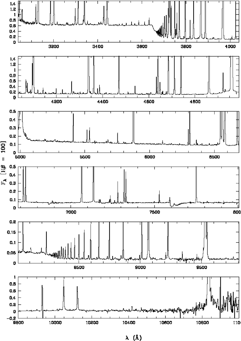
Figure 1: CCD spectra of NGC 7009 from 3040 to 11,000 Å. Flux is normalized such that H$\beta$ = 100. Extinction has not been corrected for.

3 Emission line identification

Once the data have been reduced and high-quality 1-D spectra extracted, what follows is the most tedious and time-consuming process: emission line identifications. Three steps are involved in this procedure: (1) We first identify the strong (and obvious) emission lines manually, using the traditional empirical method, aided by available atomic transition data. Lists of identified emission lines in spectra of PNe published in the literature are also used. (2) We then use the technique of multi-Gaussian fitting to deblend the possible lines blended with a strong feature, except for those saturated ones that have no short-exposure, unsaturated data. This step requires strenuous efforts because our spectra are of medium resolution, and most, if not all, faint emission lines (mainly ORLs) are blended with adjacent stronger features. Setting initial values for a multi-Gaussian fit is tricky, and can be more difficult when there are many, say more than ten, components in a single, broad feature. (3) After a complete emission line list has been generated after completing multi-Gaussian fitting across the whole spectrum, further identification is carried out with the computer-aided emission line identification code emili, originally developed by Sharpee et al. sharpee2003 (2003).

3.1 The traditional method

The usual approach of identifying emission lines in high-quality spectra is to start with lists of line identifications available in the literature for spectra of objects of similar nature. It is generally necessary to manually work through various multiplet tables and line lists in order to arrive at an identification that makes physical sense in terms of the wavelength agreement with the laboratory value, anticipated intensity, and the presence or absence from the same multiplet or from the same ion. This process, which has been referred to as the traditional approach, is both tedious and prone to be incomplete (Sharpee et al. sharpee2003 2003).

NGC 7009 is an evolved medium-excitation PN exhibiting an extraordinary rich and prominent ORL spectrum of heavy element ions that is hardly rivaled by any other bright PNe of similar excitation class. Hitherto, fairly complete emission line identifications covering the whole optical wavelengths have been carried out for a few bright objects, including the high excitation class PN NGC 7027 (Zhang et al. 2005a ) and the low excitation class PN IC 418 (Sharpee et al. sharpee2003 2003; Sharpee et al. sharpee2004 2004), amongst others. For NGC 7027, a total of 1174 identified emission lines have been tabulated, including 739 isolated features and more than two hundred blended ones without individual flux estimates. For IC 418, a total of 807 emission lines are listed, including 624 with solid identifications and another 72 with possible identifications. While the physical conditions in those two PNe differ from those of NGC 7009, we have found their line lists useful, in particular in identifying some features that are otherwise difficult to identify manually.

Liu et al. liu1995 (1995) identified and analyzed eight O ii ORL multiplets (M1, M2, M5, M10, M12, M19, M20 and M26) belonging to the 3s – 3p and 3p – 3d transitions, about 30 measurements belonging to the 3d – 4f transition as well as eleven doubly excited (with O²⁺ parentage other than ³P) ORLs in the blue optical spectrum of NGC 7009. In the same object, Luo et al. luo2001 (2001) reported and analyzed several dozen Ne ii ORLs belonging to transitions 3s – 3p, 3p – 3d and 3d – 4f. One expects that most lines emitted by NGC 7009 are of intermediate excitation energies, and second-row elements (C, N, O and Ne) are mostly doubly ionized. Triply ionized species should exist to some extent, whereas those of even higher ionization stages must be negligible.

We use midas to process the continuum-subtracted 1-D spectra. The basic observational information, such as central wavelengths, FWHMs and fluxes (normalized to a scale where H$\beta$ = 100), of all the obvious, isolated emission features in the spectra is obtained using midas. For those features with line profiles that obviously deviate from Gaussian, e.g., features that suffer from serious blending, the peak wavelength is adopted as the central wavelength. S/N ratio for each feature is obtained by measuring the standard deviation of the local continuum near the emission feature. All the observed wavelengths are corrected for the Doppler shifts (NGC 7009 is blue-shifted by about $100$ km/s) estimated from the hydrogen Balmer and Paschen lines.

We manually identify all the isolated emission features by comparing the measured central wavelengths with laboratory values available from the atomic spectral line lists compiled by Hirata & Horaguchi hh1995 (1995), after taking into account the Doppler shifts. The line lists of Hirata & Horaguchi hh1995 (1995) include only dipole transitions. For forbidden transitions, emission line lists of other PNe (e.g. NGC 7027, IC 418) from the literature are used. For features for which we cannot find reasonable identifications in the lists of either Hirata & Horaguchi hh1995 (1995) or from the literature, online atomic transition database is used as an aid. This step of manual identification is based on wavelength matching only, and could be unreliable for some features. The measured fluxes are not used because at this stage many of lines suffer from line-blending issues. Once this first round of emission-line identification is complete, we scan through the list checking for the presence of the other components belonging to the same multiplet if one of the components is identified. About 700 isolated emission features are obtained in this preliminary line list.

3.2 Enlargement of the emission line list

The preliminary line list created above is incomplete. Since the spectra are of medium resolution, $1.5$ Å  at short wavelengths and $3.0$ Å  at longer ones, many faint ORLs are partially blended with or even entirely embedded in strong features. We check for lines that should be present but are blended and add them to the emission line list. This empirical approach should proceed with great care. We search through available atomic database, including high resolution spectra of PNe in the literature. Although the physical conditions in different PNe are different, a large number of ORLs are commonly observed, as judged from a comparison of line lists of different objects. In addition to the most recent atomic database three criteria are used to decide whether a line should be present in the spectrum and thus be included in the line list:

(1) Elemental abundances: The most abundant heavy elements are O, N, C and Ne from the second row of the table of chemical elements, thus we consider the presence of their ORLs prior to those from other less abundant elements.

(2) Components within the same multiplets: If one or several components of a given multiplet have been detected with solid identifications, we assume that the other components must also be present. Only components that are too faint to be of any significance, say more than two orders of magnitude fainter than the principal component, are neglected.

(3) Ionization potential and excitation energy: In cases where not even a single component of a given multiplet is seen, but this multiplet probably should exist as judged from its excitation energy as well as ionization potential of the emitting ion, we add the multiplet to the line list. Only components that may be of any significance are included.

The emission line list enlarged in this way may still be incomplete. Limited by the spectral resolutions and S/N’s, reliable fluxes for many faint blended lines are difficult to obtain. However, the enlarged emission line list, now containing more than 1300 transitions, has nearly doubled the size of the original preliminary one.

3.3 Multi-Gaussian fits

Many of those faint ORLs are of great value for astrophysical diagnostics. In order to obtain reliable fluxes for them, deblending is often needed. Assuming all lines have a Gaussian profile, we use multi-Gaussian fitting to deblend the lines using procedures in midas. The fitting proceeds from blue to red wavelengths and covers the whole wavelength range (3040 – 11,000 Å) of the continuum-subtracted 1-D spectra, with each fit covering a spectral segment of about 20–30 Å  at short wavelengths (FWHM $\sim$ 1.5 Å) and about 50–60 Å  at long wavelengths (FWHM $\sim$ 3.0 Å). Much wider spectral segments are not favored because: (1) A wide spectral range often contains many emission components. Fitting the whole range in a single go will involve a large number of free parameters and thus may result in large uncertainties in the output. (2) The maximum number of components that midas can handle in a single multi-Gaussian fit is 16. The fit may also diverge if too many components crowd in a narrow wavelength range with adjacent lines of wavelength difference $\Delta\lambda<$ 0.5 Å.

For each segment fitted, we make sure that its blue and red ending points are equal or close to the local continuum level as judged by eyes. If several broad features are partially blended with each other and cover a wide spectral range, we split them into two smaller ones and the split point is chosen where the separation of the features is the largest. This is also judged by eyes.

For each multi-Gaussian fit to a spectral segment we first set the initial values for the parameters of each Gaussian component – height (CCD pixel value), central wavelength and width (i.e. FWHM). In general, all Gaussian components considered in a given fit are assumed to have the same line width, and the wavelength differences between individual components are fixed to their known laboratory values. Even if the initial values have been set with care, several tries are often needed before the program converges and reasonable fitting results are obtained. Fig. 2 shows the Gaussian profile fits to the spectral range 4625 – 4680 Å, where the O ii M1 lines locate. Some specific cases are noted below:

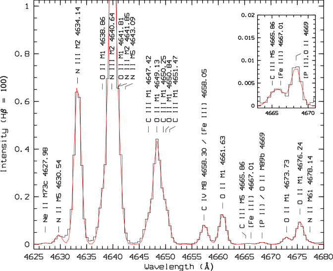
Figure 2: Spectrum of NGC 7009 from 4625 to 4680 Å showing the O ii M1 lines and other blended emission features. The continuous curve is the sum of Gaussian profile fits. The inset zooms in the weak features of [Fe iii] $\lambda$4667.01, which is blended with C iii M5 3p^′ 3P₂ – 3s^′ 3P${}^{\rm o}_{2}$ $\lambda$4665.86, and O ii M89b 4f D[2]${}^{\rm o}_{5/2}$ – 3d ²D_3/2 $\lambda$4669.27, which is blended with [P ii] 3p^2 1S₀ – 3p^2 3P₁ $\lambda$4669.25 and contributes about 40 per cent to the total flux of the blend at $\lambda$4669. Continuum has been subtracted and fluxes normalized such that H$\beta$ = 100. Extinction has not been corrected for.

(1) For a blended feature, the wavelength of the strongest component can be easily estimated. For the other fainter blended components, we fix their wavelengths relative to those stronger ones, utilizing their known laboratory wavelengths. All components are assumed to have the same FWHM. There are cases where the strongest emission component obviously deviates from a Gaussian profile. In such case we set a large FWHM to it while keeping the Gaussian assumption.

(2) For cases where several faint lines blend with a strong one with close wavelengths, say $\Delta\lambda$ $<$ 0.5 Å, accurate fluxes are almost impossible to obtain even with multi-Gaussian fitting. In such cases fluxes of fainter lines are estimated from the ionic abundances (often deduced from lines free of serious blending) using available atomic data, i.e. the effective recombination coefficients for recombination lines, and collisional strengths for forbidden lines. If a faint line contributes little, say less than 5 per cent, to the total intensity of the strong feature, we assume that the faint line is negligible.

Fig. 3 is an example illustrating the case of deblending the He i $\lambda$4026 feature. Here the N ii M39b 4f 2[5]₄ – 3d ³F${}^{\rm o}_{3}$ $\lambda$4026.08 and O ii M50b 4f F[3]${}^{\rm o}_{5/2}$ – 3d ⁴F_3/2 $\lambda$4026.31 lines are blended with the stronger He i M18 5d ³D – 2p ³P^o $\lambda$4026.20 line, with wavelength differences less than 0.5 Å. Also embedded in this feature are the He ii 4.13 13g ²G – 4f ²F^o $\lambda$4025.60 and He i M54 7s ¹S₀ – 2p ¹P${}^{\rm o}_{1}$ $\lambda$4023.99 lines.

Fluxes of the blended N ii $\lambda$4026.08 and O ii $\lambda$4026.31 lines are estimated from the N ii and O ii effective recombination coefficients calculated by Fang et al. fang2010 (2010) and Storey (private communications), respectively, using the equation,

$$\frac{I\left(\lambda\right)}{I\left({\rm H}\beta\right)}=\frac{\alpha_{\rm eff}\left(\lambda\right)}{\alpha_{\rm eff}\left({\rm H}\beta\right)}\frac{\lambda}{4861}\frac{{\rm X}^{+}}{{\rm H}^{+}},$$ (2)

where $\alpha_{\rm eff}(\lambda)$ and $\alpha_{\rm eff}({\rm H}\beta)$ are the effective recombination coefficients for the emission line $\lambda$ and H$\beta$ respectively, and X⁺/H⁺ the ionic abundance ratio (N²⁺ for the N ii line and O²⁺ for the O ii line). N²⁺/H⁺ and O²⁺/H⁺ abundance ratios are adopted from Liu et al. liu1995 (1995). Here we assume $T_{\mathrm{e}}$ = 1000 K, as diagnosed from N ii and O ii recombination lines, and $N_{\mathrm{e}}$ = 4300 cm^-3, the average electron density of NGC 7009 deduced from optical CEL ratios (Section 4). Details for the derivations of $T_{\mathrm{e}}$ based on ORLs will be presented in a subsequent paper. The fluxes of the blended N ii $\lambda$4026.08 and O ii $\lambda$4026.31 lines thus estimated contribute, respectively, 0.74 and 0.09 per cent to the He i $\lambda$4026 feature.

For the He ii $\lambda$4025.60 line, its flux is calculated from the He⁺⁺/H⁺ abundance ratio using the hydrogenic recombination theory of Storey & Hummer sh1995 (1995), with $T_{\mathrm{e}}$ and $N_{\mathrm{e}}$ assumed to be 10,000 K and 10,000 cm^-3, respectively. The estimated He ii line flux contributes 5.7 per cent to the He i $\lambda$4026 feature. The contribution of the He i $\lambda$4023.99 line is estimated from the Case B predictions of Brocklehurst brocklehurst1972 (1972), and it amounts about 0.66 per cent. In the latter case, we assume $T_{\mathrm{e}}$ = 5000 K, as is derived from the He i $\lambda$7281/$\lambda$6678 line ratio, and $N_{\mathrm{e}}$ = 10,000 cm^-3.

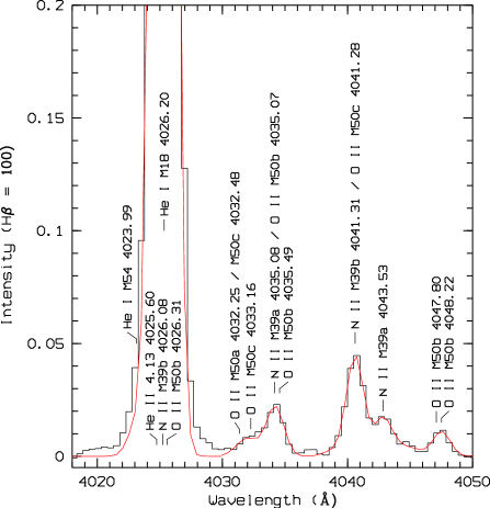
Figure 3: Spectrum of NGC 7009 from 4018 to 4050 Å showing the emission lines identified in this wavelength range. Here the strongest emission feature is the He i M18 $\lambda$4026.20 line, with at least four weak lines blended with it: He ii 4.13 $\lambda$4025.60, N ii M39b $\lambda$4026.08, O ii M50b $\lambda$4026.31 and He i M54 $\lambda$4023.99. Other emission lines present in this wavelength range, mostly N ii and O ii permitted lines, are also marked. The continuous curve represents the sum of multi-Gaussian fits. The spectrum has been continuum subtracted and flux normalized such that H$\beta$ = 100. Extinction has not been corrected for.

(3) There are cases where several faint ORLs blend together and their wavelengths do not differ much. Such feature often exhibits an irregular spectral shape, where only the relatively stronger ones can be easily discerned from the obvious peaks. In order to estimate fluxes for the fainter ones, we resort to theoretical atomic data. If the components belong to the same multiplet, their relative intensities are set to equal to the predicted values, i.e., $I(\lambda_{1})$ : $I(\lambda_{2})$ : … = $\alpha_{\rm eff}(\lambda_{1})$/$\lambda_{1}$ : $\alpha_{\rm eff}(\lambda_{2})$/$\lambda_{2}$ : …, where $\alpha_{\rm eff}(\lambda_{i})$ is the effective recombination coefficient of the blended component $i$, and $I(\lambda_{i})$ its intensity. The effective recombination coefficients adopted here are calculated assuming appropriate physical conditions ($T_{\mathrm{e}}$ and $N_{\mathrm{e}}$) under which ORLs are emitted. For NGC 7009, we assume $T_{\mathrm{e}}$ = $1000$ K and $N_{\mathrm{e}}$ = 4300 cm^-3. Here 4300 cm^-3 is the average electron density deduced in Section 4. Components predicted to have intensities negligible compared to others, are ignored. Fig. 4 shows a very broad feature between the wavelength range 4270 – 4280 Å formed by more than ten O ii lines from the 4f – 3d transition array blended together. Within this broad feature, the strongest component is M67a 4f F[4]${}^{\rm o}_{9/2}$ – 3d ⁴D_7/2 $\lambda$4275.55 with a fitted intensity of 0.11 (on a scale where H$\beta$ = 100). Fluxes of other components are estimated from the O ii effective recombination coefficients of Storey (2008), and the values are 10^-4 of H$\beta$ flux or lower.

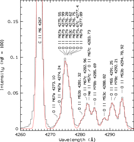
Figure 4: Spectrum of NGC 7009 from 4260 to 4298 Å. The very broad emission feature at 4275 Å  which is formed by more than ten O ii ORLs from the 4f – 3d transition array blended together, is clearly seen, with positions and wavelengths of the components labeled.

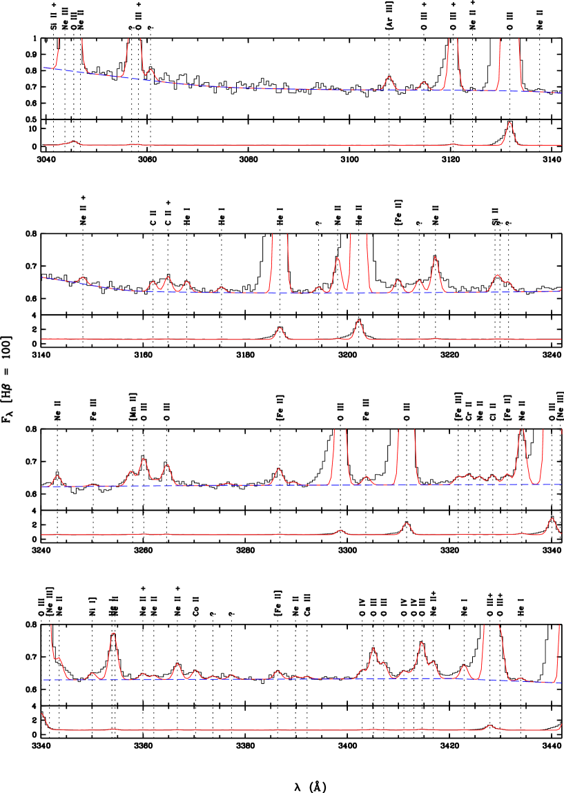
Figure 16: Spectrum of NGC 7009. A “$+$” attached to a line identification means that the line is blended with other emission features. The red solid curve is the sum of multi-Gaussian fits to the emission lines; the blue dashed line represents the continuum.

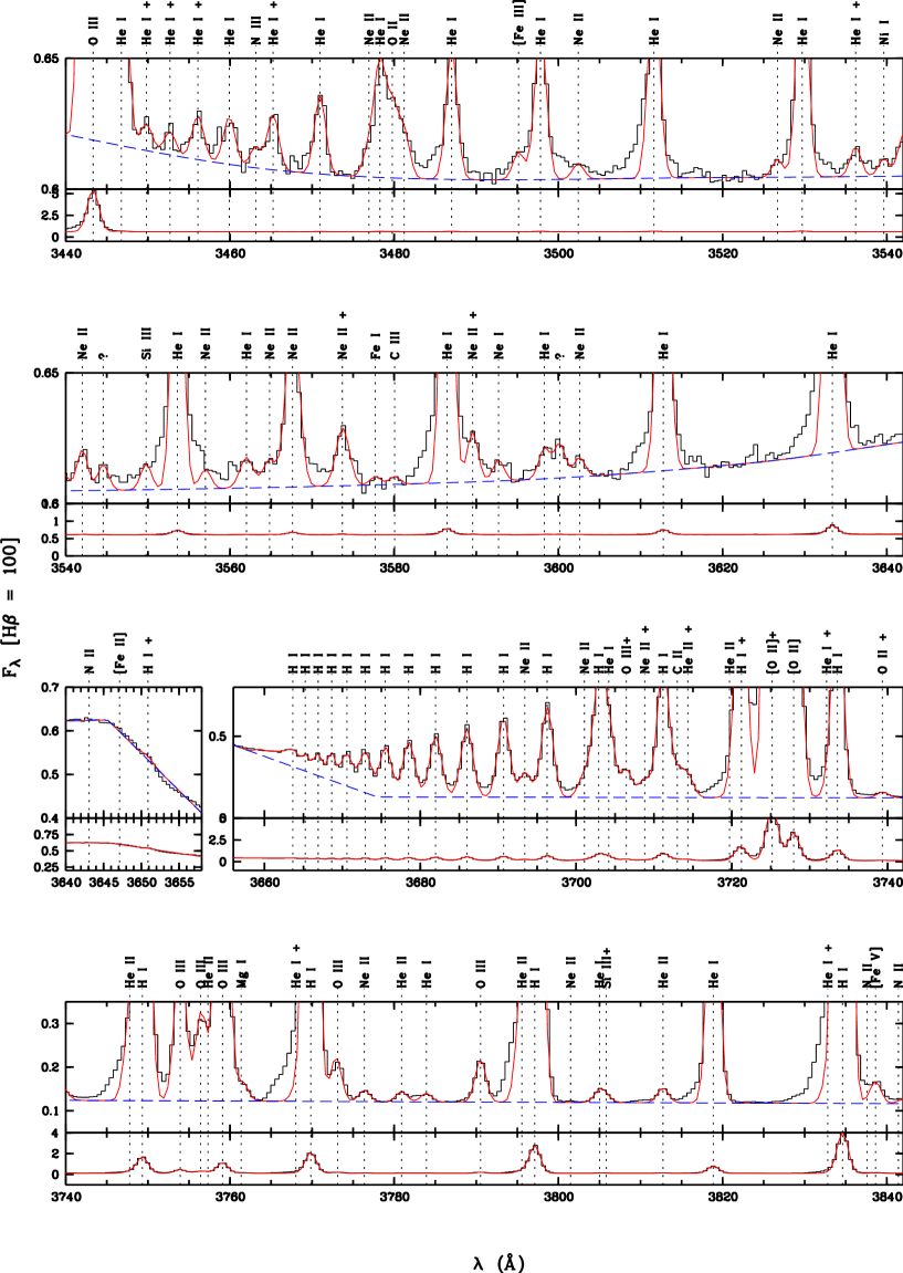
Figure 16: Continued.

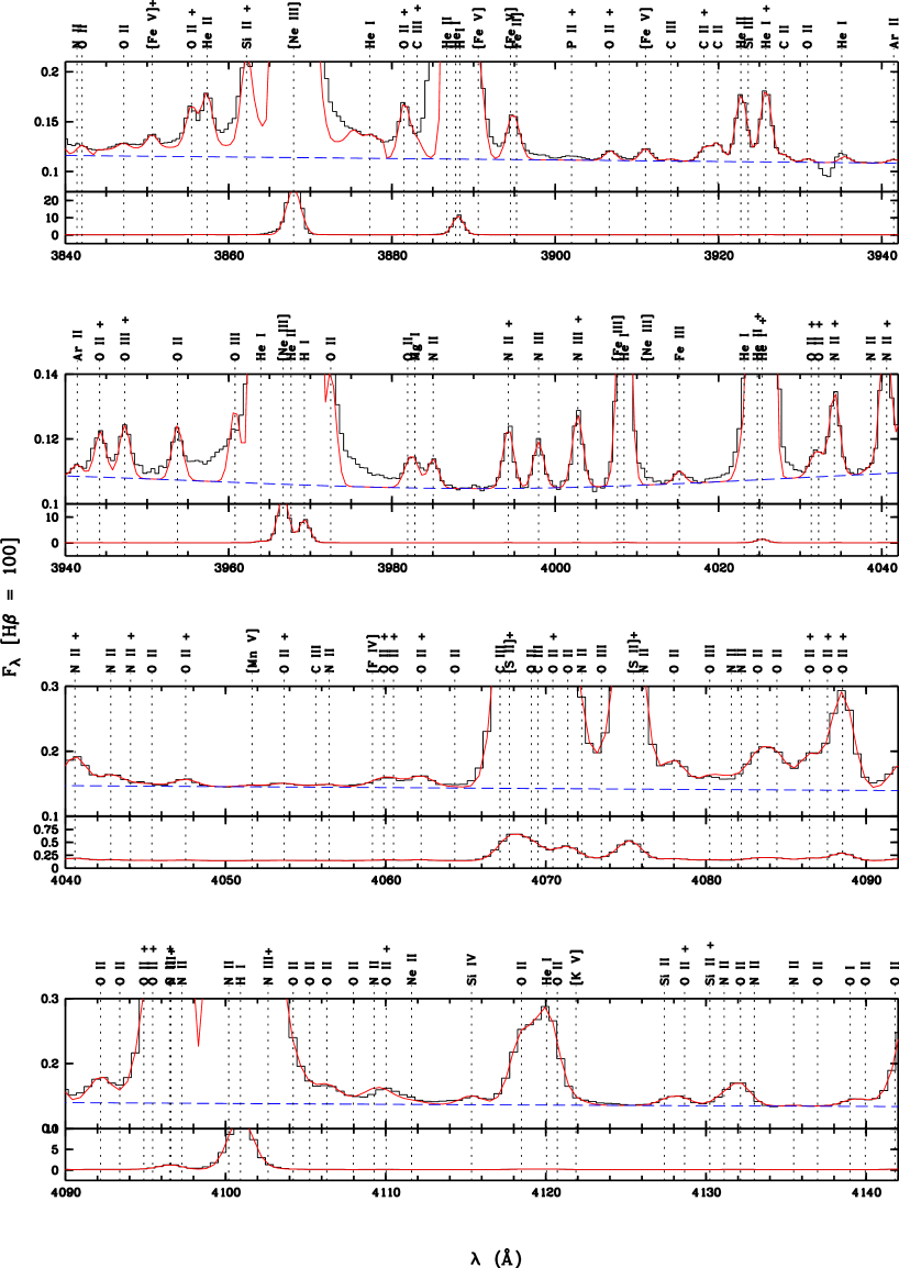
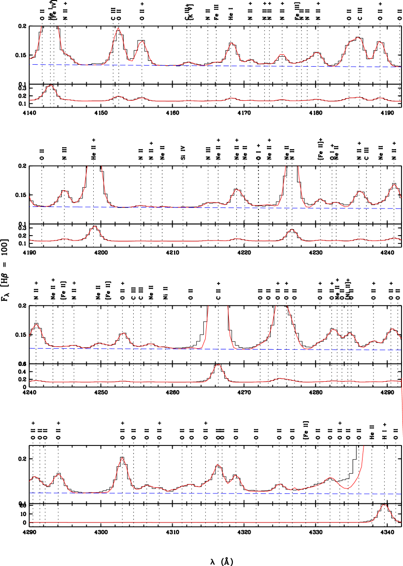
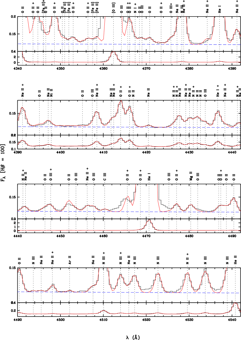
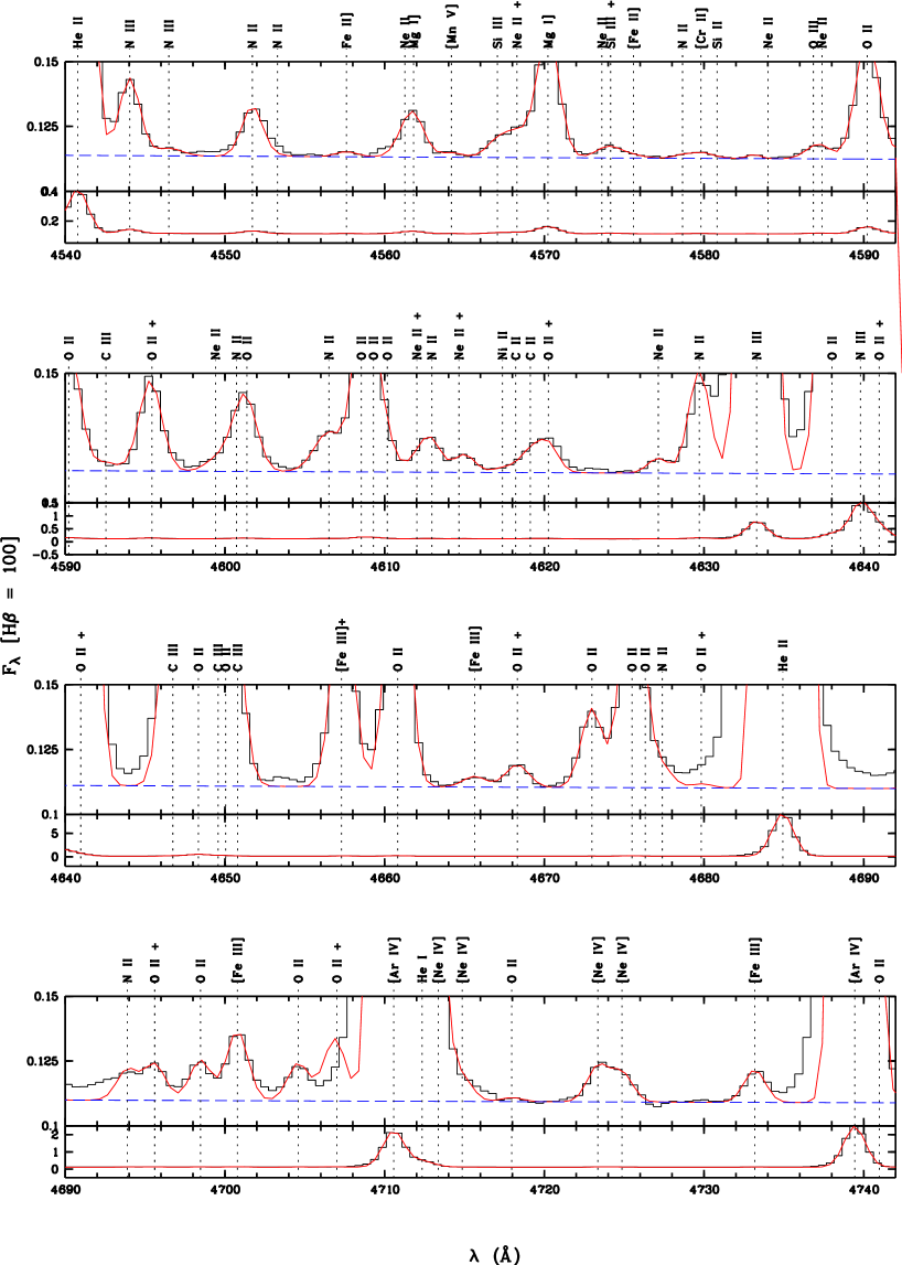
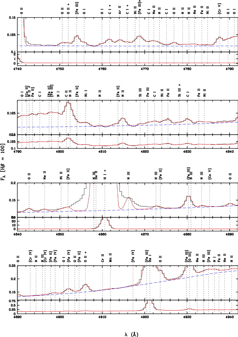
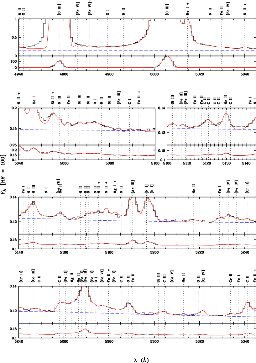
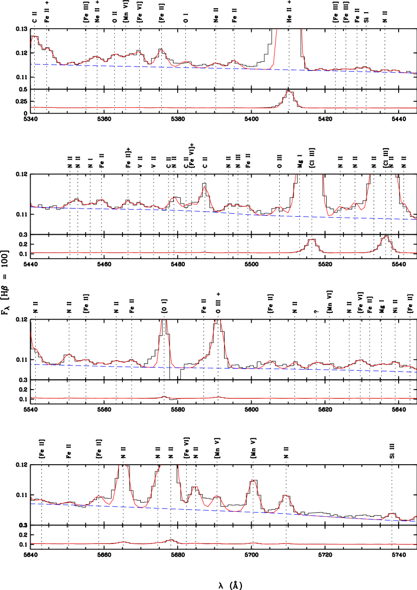
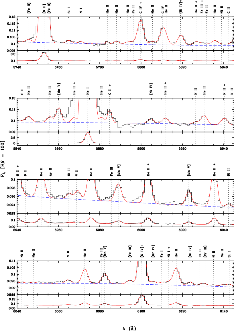
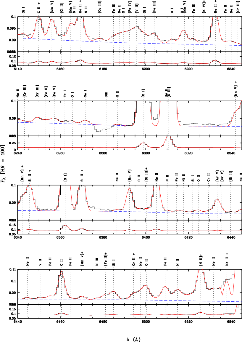
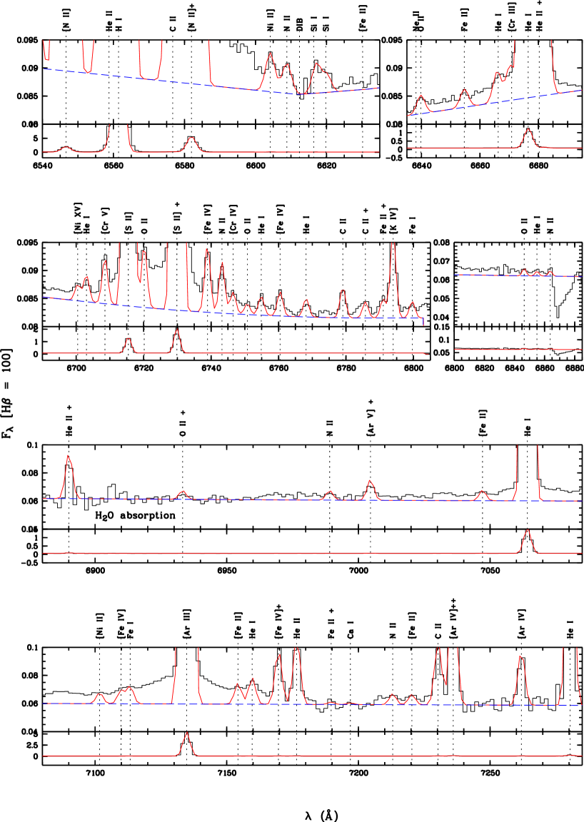
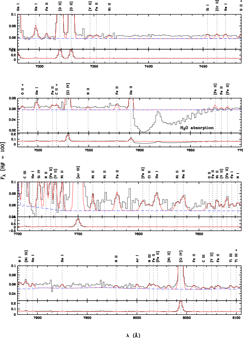
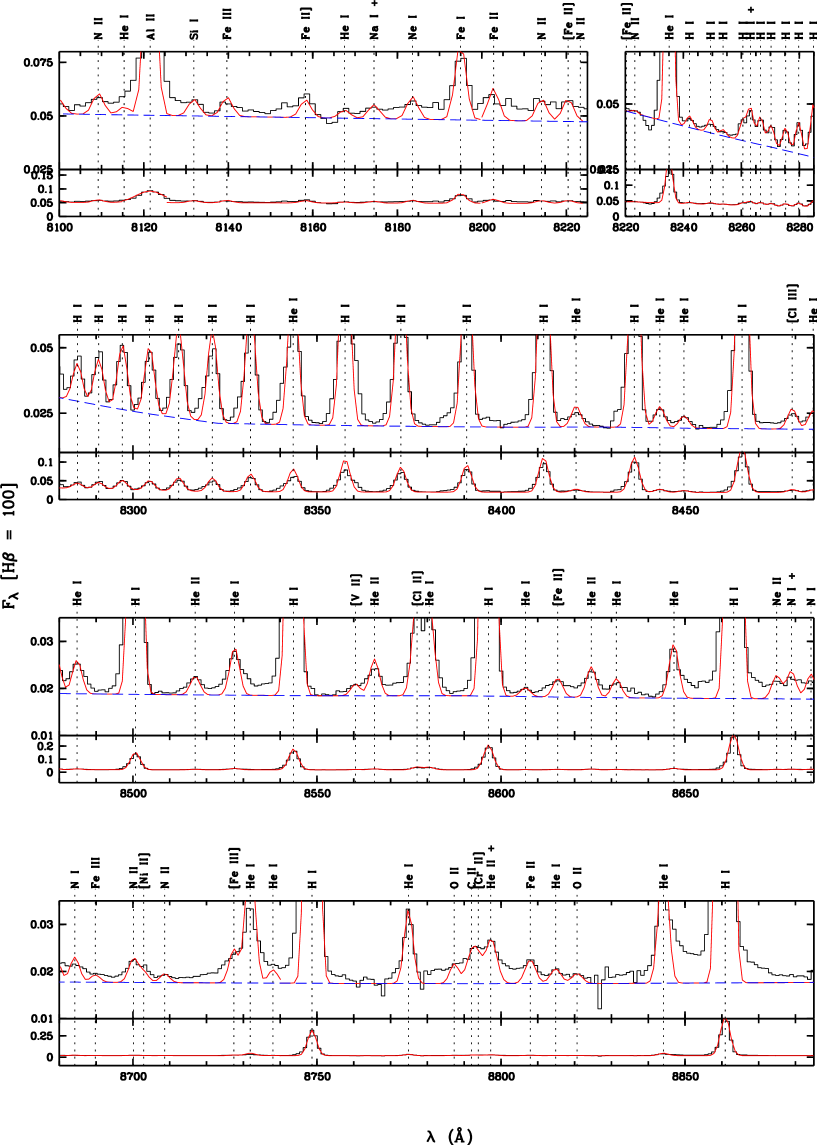
Figure 16: Continued.

Figure 16: Continued.

Figure 16: Continued.

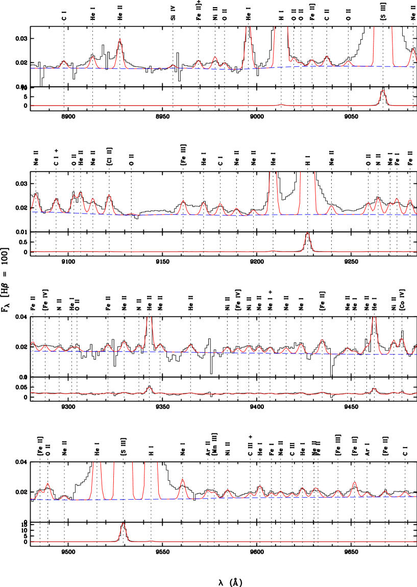
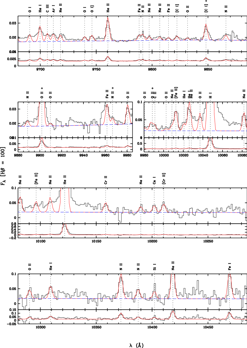
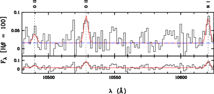
Figure 16: Continued.

The above cases illustrate the procedure that we deblend the spectra of NGC 7009 and estimate the contributions of the blended faint lines whose reliable measurements are difficult. We obtain an enlarged line list containing 1440 individual transitions, 169 of which are estimated from the available atomic data and thus have large uncertainties in their fluxes. The sum of all the multi-Gaussian fits is overplotted on the observed spectrum in Fig. 16 for comparison.

3.4 Finalization of the line list

Up to this stage, the emission line list remains preliminary, even though a large number of faint lines have been added. The identifications are done manually and may contain spurious ones, especially for those ‘isolated’ features without any other corroborative components from the same multiplet. Care must also be exercised for those that appear only in the line list of NGC 7009. Further more, the atomic database used could be incomplete, or there are more than one candidate transitions for the observed feature. A more systematic approach to line identification is needed to generate reasonable results for all emission features that are either detected or deblended properly, if necessary. Here the emission line identification code, emili, has been used to aid and clarify identifications of faint emission lines. Technic details of emili and its operation are documented in Sharpee et al. sharpee2003 (2003). Previously mentioned in Section 3.3, the intensities of a number of blended faint lines (mainly ORLs) are simply estimated from the atomic data (e.g. effective recombination coefficients) at assumed $T_{\mathrm{e}}$’s and $N_{\mathrm{e}}$’s and these estimated intensities could be of large uncertainties. These lines are excluded from the input list of the emili code, and henceforth referred to simply as estimated lines.

emili reads in the basic information (wavelengths and errors, line widths in velocity, and line intensities, etc.) of the 1271 emission transitions in the line list we have constructed, searches for all the possible candidates in the atomic transition database for each of those input transitions and decides which candidate matches the observation best. emili automatically applies the same logic that is used in the traditional manual identification of spectral lines, working on a list of measured lines and a database of known transitions, and trying to find identifications based on wavelength agreement and relative computed intensities of putative identifications, and on the presence of other confirming lines from the same multiplet or ion.

An analysis of the code output shows: (1) For strong lines, e.g., most CELs, hydrogen lines, relatively strong helium lines, and some relatively strong ORLs emitted by C, N, O and Ne ions, the code output agrees well with the empirical identifications obtained manually. (2) For most faint ORLs emitted by C, N, O and Ne ions as well as by ions of the third-row elements (e.g., Mg ii, Si ii, Si iii, etc.) identifications returned by the code generally agree with empirical identifications, except for a few faint lines with fluxes $\simeq$ 10^-4 to 10^-5 times the H$\beta$. For this small number of lines, emili gives identifications different from the original assignments, and this adds ambiguity to their identifications. For these lines, we search the whole line list and choose the candidate that have highest number of solidly identified lines from the same multiplet or from the same ion. (3) A few dozen emission lines are unidentified. We attribute this to either the lack of relevant atomic data, or large errors from the multi-Gaussian fits, or spurious features. For transitions that have alternative identifications given by emili, we list all the candidates and mark them as blends (the fourth column of Table LABEL:linelist). In total, there are 1170 identified transitions in the final emission line list plus 28 unknown features, 235 alternative identifications given by emili and 73 questionable ones. Most of the latter ones are identified as Ne i, Fe i, Co i, Ni i and etc. The identifications as well as the observed and dereddened line fluxes (on a scale where H$\beta$ is 100) are presented in Table LABEL:linelist. The 169 blended faint lines, whose intensities are simply estimated from atomic data, are also included in the line list, and their flux errors (the last column of Table LABEL:linelist) could be large and are labeled by “:”. In Fig. 16, identifications of all lines present in the spectrum are marked.

4 Plasma diagnostics

Electron densities and temperatures are deduced from optical CEL ratios of heavy element ions. Also derived are temperatures from the hydrogen continuum Balmer and Paschen discontinuities, and from the He i and He ii recombination spectrum, the $N_{\mathrm{e}}$’s from the Balmer and Paschen decrements. The enhancement of the [N ii], [O ii] and [O iii] auroral lines contributed by recombination excitation is discussed, and estimation of the enhancement is provided.

4.1 $T_{\mathrm{e}}$’s and $N_{\mathrm{e}}$’s from CELs

The spectrum of NGC 7009 reveals many CELs, useful for nebular electron density and temperature diagnostics and abundance determinations. Adopting the atomic data from the references given in Table 2 and solving the level populations for multilevel ($\geq~{}5$) atomic models, we have determined electron temperatures and densities from a variety of CEL ratios. The results are listed in Table 3. Electron temperatures were derived assuming a constant electron density of $\log$ $N_{\mathrm{e}}$ = 3.633 (cm^-3), or 4290 cm^-3, the average value yielded by the four density-sensitive CEL diagnostic ratios, [O ii] $\lambda$3726/$\lambda$3729, [S ii] $\lambda$6731/$\lambda$6716, [Ar iv] $\lambda$4740/$\lambda$4711 and [Cl iii] $\lambda$5537/$\lambda$5517. The four [Fe iii] line ratios, $\lambda$4733/$\lambda$4754, $\lambda$4701/$\lambda$4733, $\lambda$4881/$\lambda$4701 and $\lambda$4733/$\lambda$4008, yield much higher electron densities for $T_{\mathrm{e}}$ = 10,020 K, the average temperature deduced from a number of optical CEL ratios. We have thus ignored densities yielded by the [Fe iii] line ratios in calculating the average electron density. A plasma diagnostic diagram based on CEL ratios is plotted in Fig. 5. The temperature diagnostic ratio, [O i] ($\lambda$6300 + $\lambda$6363)/$\lambda$5577 is not used because of poor sky subtraction for the auroral line $\lambda$5577, making its intensity quite unreliable.

The [O ii] nebular-to-auroral line ratio ($\lambda$7320 + $\lambda$7330)/$\lambda$3729 yields an electron temperature of about 19,000 K, which is abnormally high, if one assumes an electron density of Log$N_{\mathrm{e}}$ = 3.674 (Table 3), as yielded by the [O ii] $\lambda$3726/$\lambda$3729 line ratio. Here we assume $N_{\mathrm{e}}$ = 10,000 cm^-3 for [O ii], and then the [O ii] nebular-to-auroral line ratio yields a temperature of 9850 K, which is quite reasonable.

Table 2: References for CEL atomic data.

ion	Transition probabilities	Collision strengths
N ii	Nussbaumer & Rusca nr1979 1979	Stafford et al. stafford1994 1994
O i	Baluja & Zeippen bz1988 1988	Berrington berrington1988 1988
O ii	Zeippen zeippen1982 1982	Pradhan pradhan1976 1976
O iii	Nussbaumer & Storey ns1981 1981	Aggarwal aggarwal1983 1983
Ne iii	Mendoza mendoza1983 1983	Butler & Zeippen bz1994 1994
S ii	Mendoza & Zeippen mz1982b 1982	Keenan et al. keenan1996 1996
	Keenan et al. keenan1993 1993
S iii	Mendoza & Zeippen mz1982a 1982	Mendoza mendoza1983 1983
Cl iii	Mendoza mendoza1983 1983	Mendoza mendoza1983 1983
Ar iii	Mendoza & Zeippen mz1983 1983	Johnson & Kingston jk1990 1990
Ar iv	Mendoza & Zeippen mz1982b 1982	Zeippen et al. zeippen1987 1987
Fe iii	Nahar & Pradhan np1996 1996	Zhang zhang1996 1996

Table 3: Plasma diagnostics.

ID	Diagnostic	Result
		$T_{\mathrm{e}}$ [K]
1	[N ii] ($\lambda$6548 + $\lambda$6584)/$\lambda$5754	10,780a
2	[O iii] ($\lambda$4959 + $\lambda$5007)/$\lambda$4363	10,940
3	[S iii] ($\lambda$9531 + $\lambda$9069)/$\lambda$6312	11,500
4	[O ii] ($\lambda$7320 + $\lambda$7330)/$\lambda$3729	9850b
5	[O i] ($\lambda$6300 + $\lambda$6363)/$\lambda$5577	–c
6	[Ar iii] $\lambda$7135/$\lambda$5192	10,050
	[O iii] $\lambda$4959/$\lambda$4363	9810
	[O iii] (52$\mu$m + 88$\mu$m)/$\lambda$4959	9260
	[Ne iii] (15.5$\mu$m + 36$\mu$m)/($\lambda$3868 + $\lambda$3967)	9010
	[S ii] ($\lambda$6717 + $\lambda$6731)/($\lambda$4069 + $\lambda$4076)	9770
	Average optical CEL temperature	10,020d
	He i $\lambda$7281/$\lambda$5876	3850
	He i $\lambda$7281/$\lambda$6678	5100
	He i $\lambda$5876/$\lambda$4471	4360
	He i $\lambda$6678/$\lambda$4471	9690
	H i BJ / H11	6420
	H i PJ / P11	6750$\pm$160
	He i Jump at 3421 Å	7800$\pm$200
	He ii Jump at 5694 Å	11,000$\pm$2000
		$N_{\mathrm{e}}$ [cm-3]
7	[Ar iv] $\lambda$4740/$\lambda$4711	4890
8	[Cl iii] $\lambda$5537/$\lambda$5517	3600
9	[S ii] $\lambda$6731/$\lambda$6716	4100
10	[Fe iii] $\lambda$4733/$\lambda$4754	64,560
11	[Fe iii] $\lambda$4701/$\lambda$4733	22,860
12	[Fe iii] $\lambda$4881/$\lambda$4701	93,330
13	[Fe iii] $\lambda$4733/$\lambda$4008	–e
14	[O ii] $\lambda$3726/$\lambda$3729	4720
	Adopted optical CEL density	4290
	[O iii] 52$\mu$m/88$\mu$m	1260
	[Ne iii] 15.5$\mu$m/36$\mu$m	11,480
	H i Balmer decrement	3000
	H i Paschen decrement	1000$\sim$3000

^a

Probably unreliable. Here an electron density Log$N_{\mathrm{e}}$ = 4.0 is assumed. The intensity of the auroral line $\lambda$5754 has been corrected for the contribution from recombination excitation (c.f. Section 4.3), which amounts to 9.5 per cent.

^b

Assuming $LogN_{\mathrm{e}}$ = 4.0. The intensity of the two auroral lines $\lambda\lambda$7320, 7330 have been corrected for the contribution by recombination excitation (c.f. Section 4.3), which is about 13 per cent.

^c

The intensity of the $\lambda$5577 line is unreliable due to poor sky subtraction.

^d

Average temperature derived from the [O ii], [O iii], [S iii] and [Ar iii] nebular-to-auroral line ratios.

^e

The loci of this diagnostic delineates very high temperatures, from 11,500 to 19,800 K for the density range 3.06 $\leq$ Log$N_{\mathrm{e}}$ $\leq$ 3.61.

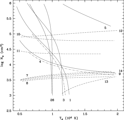
Figure 5: Plasma diagnostic diagram. Each curve is labeled with an ID number given in Table 3. The solid curves are temperature-sensitive diagnostics, and the dashed curves are density-sensitive diagnostics. The dash-dot curves represent temperature diagnostics of [N ii] (labeled as 1) and [O ii] (labeled as 4), after the contributions by recombination excitation to the auroral lines have been corrected for, whereas the solid curves represent those without corrections.

4.2 Recombination excitation of the [N ii], [O ii] and [O iii] auroral lines

In NGC 7009, most N and O atoms are in their doubly ionized stages. Recombination of N²⁺ and O²⁺ can be important in exciting the weak [N ii] $\lambda$5754 auroral line and the [O ii] auroral and nebular lines $\lambda\lambda$7320, 7330, and $\lambda\lambda$3726, 3729, leading to apparent high electron temperatures from the ($\lambda$6548 + $\lambda$6584)/$\lambda$5754 and ($\lambda$7320 + $\lambda$7330)/$\lambda$3727 ratios (Rubin rubin1986 1986). Similarly, the [O iii] auroral line $\lambda$4363 could be also enhanced by recombination, leading to an overestimated $T_{\mathrm{e}}$. Here we estimate the contribution by recombination using the empirical fitting formulae [Equations (1), (2) and (3) in their paper] given by Liu et al. liu2000 (2000), which are derived from the recombination coefficients and transition data for the meta-stable levels of N⁺, O⁺ and O²⁺ ions. The three equations are as follows:

$$\frac{I_{\mathrm{R}}(\lambda~{}5754)}{I(\rm{H}\beta)}=3.19t^{0.30}\times\frac{\rm{N}^{2+}}{\rm{H}^{+}},(0.5\leq~{}t~{}\leq 2.0),$$ (3)

$$\frac{I_{\mathrm{R}}(\lambda~{}7320+\lambda~{}7330)}{I(\rm{H}\beta)}=9.36t^{0.44}\times\frac{\rm{O}^{2+}}{\rm{H}^{+}},(0.5\leq~{}t~{}\leq 1.0),$$ (4)

and

$$\frac{I_{\mathrm{R}}(\lambda~{}4363)}{I(\rm{H}\beta)}=12.4t^{0.59}\times\frac{\rm{O}^{3+}}{\rm{H}^{+}},$$ (5)

where $t$ = $T_{\mathrm{e}}$/10⁴ K.

For the [N ii] $\lambda$5754 auroral line, we estimate the recombination-contributed intensity of about 0.037 [$I(\rm{H}\beta)$ = 100], which amounts to 9.5 per cent of the observed intensity of $\lambda$5754. Here we use the N²⁺/H⁺ abundance ratio derived from the [N iii] 57$\mu$m far-IR line obtained from the ISO/LWS observation by Liu et al. liu2001 (2001). The temperature range that Eq. (4) can be applied is 5000 $\leq\,T_{\mathrm{e}}\,\leq$ 20,000 K. Here we adopt the average $T_{\mathrm{e}}$ of NGC 7009 deduced from CEL diagnostic ratios, which is about 10,020 K (Table 3), to calculate the contribution by recombination. If instead we use the N²⁺/H⁺ abundance ratio derived from the UV N iii] $\lambda$1747 line, with the observed flux from the IUE observation by Perinotto & Benvenuti pb1981 (1981), then we find that the recombination contributes about 4.5 per cent to the total intensity of $\lambda$5754. We assume that the N²⁺/H⁺ abundance from far-IR line is more reliable. Subtracting the flux contributed by the recombination excitation, we obtain a ($\lambda$6584 + $\lambda$6548)/$\lambda$5754 ratio that is about 9.5 per cent higher than the value before the correction, and that brings the resultant electron temperature from original 12,100 K down to now 10,780 K, assuming an electron density of 10,000 cm^-3. If we use the average electron density 4290 cm^-3, the corrected [N ii] nebular-to-auroral line ratio then yields a temperature of 11,520 K.

For the [O ii] auroral lines $\lambda\lambda$7320, 7330, we estimate the recombination excitation contributes an intensity of 0.303 [$I(\rm{H}\beta)$ = 100], which is about 13 per cent of their total intensity. Here the O²⁺/H⁺ abundance ratio derived from [O iii] optical CELs is used. And we use an electron temperature of 9810 K, derived from the [O iii] $\lambda$4959/$\lambda$4363 ratio. Subtracting the recombination contribution, we obtain a temperature of 9850 K from the corrected [O ii] ($\lambda$7320 + $\lambda$7330)/$\lambda$3729 ratio, with electron density assumed to be 10,000 cm^-3. The result seems reasonable, given the fact that O⁺ resides in a relatively low ionization region.

For the [O iii] auroral line $\lambda$4363, we estimate the recombination excitation contributes an intensity of 0.049 [$I(\rm{H}\beta)$ = 100], which amounts to only about 0.68 per cent of the total $\lambda$4363 intensity. This contribution is negligible. Here the O³⁺/H⁺ abundance ratio derived from the O iv] $\lambda$1403 UV line is used, with its observed flux from the IUE observations by Perinotto & Benvenuti pb1981 (1981), and electron temperature is set to be 10,020 K.

For the above three cases, the forbidden line temperatures and CEL abundances are used to calculate the intensities contributed by recombination excitation. These results are applicable for a chemically uniform nebula, and can be used to explain the apparently high temperatures yielded by the [N ii] $\lambda$5754 and [O ii] $\lambda\lambda$7320, 7330 auroral lines. For a chemically inhomogeneous nebula, for example, the model proposed by Liu et al. liu2000 (2000) to explain the long-existing discrepancies in the electron temperature diagnostics and heavy element abundance determinations in PNe and probably also in H ii regions, using recombination lines/continua on the hand and CELs on the other, the approach above may not be applicable. In their bi-abundance model, Liu et al. liu2000 (2000) suggest that the nebula contains a “cold”, H-deficient and metal-rich component, where most of the observed fluxes of heavy element ORLs arise. The CELs are mainly emitted by the hot ambient plasma. Plasma diagnostics with the aid of newly calculated effective recombination coefficients during the past decade shows that this “cold” component has electron temperatures much lower than the forbidden line temperatures by nearly an order of magnitude, reaching, in some PNe, as low as 1000 K or even lower (Liu et al. 2006a ). The heavy element abundances of this “cold” component are much higher than those derived from CELs by a factor of 2 to 10, and up to 2 orders of magnitude in the most extreme case (Liu et al. 2006a ). Evidence in favor of this bi-abundance model has been provided by a number of ORL surveys in the past decade.

The “cold” and H-deficient (metal-rich) component postulated by Liu et al. liu2000 (2000) may also contribute to the auroral lines of [N ii] and [O ii]. If we adopt an electron temperature for the “cold” component of plasma, say 1000 K, and N²⁺/H⁺, O²⁺/H⁺ and O³⁺/H⁺ abundance ratios derived from ORLs, then the contribution of recombination excitation to the [N ii] $\lambda$5754 line is 0.061 [$I(\rm{H}\beta)$ = 100], about 15.6 per cent of its observed value, higher than the percentage of 9.5 derived above using the N²⁺/H$+$ abundance ratio derived from the [N iii] 57$\mu$m. For the [O ii] $\lambda\lambda$7320, 7330 auroral lines, the contribution is 22 per cent, also much higher than the value estimated above. For the [O iii] $\lambda$4363 auroral line, the recombination excitation contributes about 15 per cent to its total intensity, if $T_{\mathrm{e}}$ = 1000 K and the O³⁺/H⁺ abundance ratio derived from the O iii M8 $\lambda$3265 line is adopted.

From the discussion above, it is clear that, depending on the physical models assumed, the exact amounts of the recombination contribution to the [O ii] and [N ii] auroral lines remain uncertain, and thus the electron temperatures derived from them (and consequently ionic abundances derived from CELs). The difficulty is that, in the scenario of the bi-abundance model, without resort detailed modeling, it is impossible to separate the contributions from the two components of plasma of vastly different physical conditions and chemical composition to the observed fluxes of emission lines, CELs or ORLs likewise.

4.3 $T_{\mathrm{e}}$ and $N_{\mathrm{e}}$ from the H i Balmer recombination spectrum

Together with the temperatures and densities derived from CEL ratios, Table 3 also gives the Balmer jump temperature derived from the ratio of the nebular continuum Balmer discontinuity at 3646 Å  to H11 $\lambda$3770, which is defined as [$I_{\mathrm{c}}(\lambda 3643)$ $-$ $I_{\mathrm{c}}(\lambda 3681)$]/$I$(H11). Here $I_{\mathrm{c}}(\lambda 3643)$ and $I_{\mathrm{c}}(\lambda 3681)$ are the nebular continua at 3643 and 3681 Å, respectively. Using the fitting formula from Liu et al. liu2000 (2000),

$$T_{\mathrm{e}}=368\times(1+0.259~{}\frac{\rm He^{+}}{\rm H^{+}}+3.409~{}\frac{\rm He^{2+}}{\rm H^{+}})(\frac{\rm BJ}{{\rm H}11})^{-3/2}~{}{\rm K},$$ (6)

we derive a Balmer jump temperature of 6490 K (Table 3). Here He⁺/H⁺ = 0.099 and He²⁺/H⁺ = 0.013, as derived, respectively, from the He i $\lambda\lambda$4471, 5876 and 6678 and from the He ii recombination line $\lambda$4686. Our Balmer jump temperature agrees within the uncertainties with that obtained by Zhang et al. zhang2004 (2004), but is much lower than the values 8000$\sim$8300 K given by Liu et al. liu1995 (1995). The difference could not be caused by the different extinction values adopted, given the small wavelength gap between the Balmer discontinuity and H 11, but is more likely due to different nebular regions being sampled. The Balmer jump temperature 6500 K is about 3300 K lower than the [O iii] forbidden line temperature $T_{\mathrm{e}}$([O iii]), and about 3500 K lower than the value of 10,020 K, yielded by a number of optical CEL ratios (Table 3).

The intensities of the high-order Balmer lines relative to H$\beta$, $I(n\rightarrow\,2,n\geq\,10)$, are sensitive to electron density $N_{\mathrm{e}}$ and thus provide a valuable density diagnostic. Unlike the Balmer discontinuity, this diagnostic is insensitive to the adopted electron temperature and can be used to probe the presence of high-density plasmas ($N_{\mathrm{e}}\geq\,10^{6}$ cm^-3). With our spectral resolution, the Balmer decrements can be measured up to $n\sim\,23$. For higher $n$, the fluxes become unreliable due to line blending. Fig. 7 shows the Balmer line intensities as a function of $n$ for 10 $\leq\,n\leq$ 24. Also overplotted in the Figure are the predicted Balmer line intensities for different densities for a fixed $T_{\mathrm{e}}$ of 6500 K deduced from the Balmer discontinuity. The predictions are calculated from the H i emissivities of Storey & Hummer sh1995 (1995). An optimization yields a Balmer decrement density of 3000 cm^-3 (Table 3). This value is about 3300 cm^-3 lower than Zhang et al. zhang2004 (2004).

Given the crowdedness of lines in the spectral region redwards of the Balmer discontinuity, where in addition to the high-order Balmer lines also fall many faint ORLs from helium and heavy elements, there are no line-free spectral windows from the Balmer discontinuity to 3745 Å, as is shown in Fig. 6. The continuum level in this spectral range is therefore estimated by linear extrapolation from longer wavelengths (Fig. 6), a method adopted by Liu et al. liu2000 (2000) in their determination of the Balmer discontinuity of the NGC 6153 spectrum. Given the short wavelength range covered (from the leftward of the Balmer discontinuity to H 11 $\lambda$3770) and the flatness of the nebular continuum, the local continuum level thus derived should be secure enough. As estimated by Liu et al. liu2000 (2000) for NGC 6153, the resultant Balmer line intensities could be accurate to a few per cent.

Multi-Gaussian fitting is performed in the continuum-subtracted spectrum to derive individual line fluxes, especially for the wavelength region near the Balmer discontinuity, where many ORLs from He i, He ii and heavy element ions are blended with the crowd of high order H i Balmer lines. H 14 $\lambda$3721.94 is partially blended with the [O ii] $\lambda$3726, in addition to the [S iii] 3p^2 1S₀ – 3p^2 3P₁ $\lambda$3721.69 line, the latter contributes about 30 per cent to the total intensity of H 14 as estimated from the multi-Gaussian fitting. A high-order He ii line 28g ²G – 4f ²F^o $\lambda$3720.41 probably also contributes to H 11, at the level less than 1 per cent. H 15 $\lambda$3711.97 is blended with two Ne ii lines M1 $\lambda$3709.62 and M5 $\lambda$3713.08, and two O iii M14 lines $\lambda$3714.03 and $\lambda$3715.08 also affect the wing of H 15. H 16 $\lambda$3703.85 is partially blended with the O iii $\lambda$3707.25, in addition to the O iii M14 $\lambda$3702.75 and He i M25 7d ³D – 2p ³P^o $\lambda$3705.00. H 17 $\lambda$3697.15 and H 18 $\lambda$3691.55 are both affected by the Ne ii M1 3p ⁴P${}^{\rm o}_{5/2}$ – 3s ⁴P_5/2 $\lambda$3694.21. For low-order Balmer lines H $n$ ($n$ = 10, 11, 12), the deblending of faint ORLs is relatively easy as the spectrum becomes less crowded. Fig. 7 shows that H 14 and H 16 may be overestimated whereas those of H 23 and H 24 underestimated.

The electron density derived from the high-order Balmer lines is 3000 cm^-3, which does not differ much from the average density 4290 cm^-3 derived from the optical CEL ratios of [O ii], [S ii], [Cl iii] and [Ar iv] (Table 3).

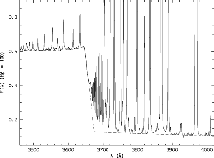
Figure 6: The near-UV spectrum of NGC 7009 from 3460 to 4020 Å, showing the nebular continuum Balmer discontinuity at 3646 Å. The ratio of the Balmer jump to H 11 $\lambda$3770 yields an electron temperature of 6490 K, about 3300 K lower than that derived from the [O iii] $\lambda$4959/$\lambda$4363 nebular-to-auroral line ratio. The dashed line is a two-part fit to the continuum, bluewards and redwards of the Balmer jump. The observed continuum level includes a small contribution from the central star. The stellar continuum is expected to be smooth over the plotted wavelength range and thus should not affect the magnitude of the observed Balmer discontinuity. The spectrum has been corrected to the rest wavelengths but not corrected for extinction, and is normalized such that $F({\rm H}\beta)$ = 100.

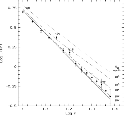
Figure 7: Observed intensities (in units where H$\beta$ = 100) of high-order Balmer lines H $n$($n$ = 10, 11, 12, …, 24) as a function of the principal quantum number $n$. The intensities of H14 and H16 may be overestimated due to blending of unknown lines, in addition to those deblended (see text for more details). The curves show the predicted Balmer decrements for a range of electron density from $N_{\mathrm{e}}$ = 10² to 10⁶ cm^-3. A constant temperature of 6500 K, derived from the nebular continuum Balmer discontinuity, has been assumed in all cases.

4.4 $T_{\mathrm{e}}$ and $N_{\mathrm{e}}$ from the H i Paschen recombination spectrum

Electron temperature is also estimated from the Paschen decrements, using

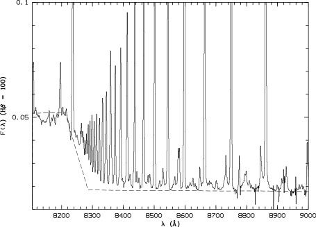
Figure 8: The red spectrum of NGC 7009 from 8105 to 9000 Å, showing the nebular continuum Paschen discontinuity at 8204 Å, as well as the Paschen decrements. The dashed line is a two-part fit to the continuum, bluewards and redwards of the Paschen jump. The observed continuum level includes a small contribution from the central star. The stellar continuum is expected to be extremely smooth over the plotted wavelength range and thus does not affect the estimate of the Paschen discontinuity. The spectrum has been corrected to the rest wavelengths but not corrected for extinction, and is normalized such that $F({\rm H}\beta)$ = 100.

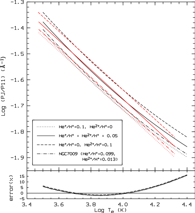
Figure 9: $Upper~{}Panel$: The Paschen discontinuity to P11 ratio, PJ/P11 $\equiv$ [$I_{\rm c}(8194)$ $-$ $I_{\rm c}(8269)$]/$I$(P11), as a function of $T_{\mathrm{e}}$, in logarithm space, for (a) He⁺/H⁺ = 0.1 and He²⁺/H⁺ = 0 (dotted line), (b) He⁺/H⁺ = He²⁺/H⁺ = 0.05 (solid line), (c) He⁺/H⁺ = 0 and He²⁺/H⁺ = 0.1 (dashed line), and (d) He⁺/H⁺ = 0.099 and He²⁺/H⁺ = 0.013 (dash-dot line), which is the case of NGC 7009. $I_{\rm c}(8194)$ and $I_{\rm c}(8269)$ are the nebular continuum fluxes at 8194 and 8269 Å, respectively, which bracket the H i Paschen discontinuity at 8204 Å  and several discontinuities of He i and He ii. Also overplotted are the red curves calculated from Eq. 7 for the four cases. $Lower~{}Panel$: Distribution of fitting errors using Eq. 7 as a function of $T_{\mathrm{e}}$ for the four cases as defined in the $upper~{}panel$. Here the fitting error is calculated from the real unit of electron temperature (K), not in logarithm space as in the $upper~{}panel$.

$$T_{\rm e}=8.72\times(1+0.52\frac{{\rm He}^{+}}{{\rm H}^{+}}+4.40\frac{{\rm He}^{2+}}{{\rm H}^{+}})(\frac{\rm PJ}{\rm P~{}11})^{-1.77}.$$ (7)

where PJ/P11 is ($I_{\rm c}(8194)$ $-$ $I_{\rm c}(8169)$)/$I$(P11), in units of Å^-1. The fitting errors given by Eq. 7 are less than 5 per cent for the temperature range 10^3.55 $\leq$ Log$T_{\mathrm{e}}$ $\leq$ 10^4.15, which is from 3550 to 14,000 K, and are less than 16 per cent for 10^3.50 $\leq$ Log$T_{\mathrm{e}}$ $\leq$ 10^4.40, as is shown in Fig. 9. The electron temperature derived from the Paschen jump for NGC 7009 is 6750$\pm$160 K (Table 3).

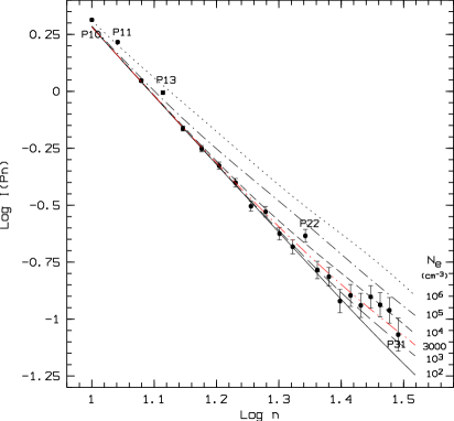
Figure 10: Observed intensities (in units where H$\beta$ = 100) of high-order Paschen lines P $n$ ($n$ = 10, 11, 12,…, 31) as a function of the principal quantum number $n$. The intensities of P11 and P13 are overestimated due to the blend of other emission lines. Also probably overestimated are Paschen lines with $n\geq\,28$. The various curves show respectively the predicted Paschen decrements for electron densities from 10² to 10⁶ cm^-3. A constant temperature of 6750 K as derived from the nebular continuum Paschen discontinuity has been assumed in all cases.

4.5 $T_{\mathrm{e}}$’s from the He i and He ii recombination spectra

Electron temperatures are derived from the intensity ratios of the He i $\lambda$4471, $\lambda$5876, $\lambda$6678 and $\lambda$7281 recombination lines, as is shown in Table 3. Zhang et al. 2005b developed an electron temperature diagnostic with the He i recombination lines, utilizing the He i line emissivities calculated by Benjamin et al. benjamin1999 (1999). Analytic formulae for the He i line emissivities were used:

$$\frac{I_{1}}{I_{2}}=\frac{a_{1}}{a_{2}}t^{b_{1}-b_{2}}{\rm exp}(\frac{c_{1}-c_{2}}{t}),$$ (8)

where $t$ = $T_{\mathrm{e}}$/10⁴ K, and $a_{i}$, $b_{i}$ and $c_{i}$ are the fitting parameters for emissivities given by Benjamin et al. benjamin1999 (1999). Eq. (8) is valid for the temperature 5000$\sim$20,000 K. For lower temperatures ($T_{\mathrm{e}}\,<\,5000$ K), Zhang et al. 2005b obtained similar fits using the He i recombination line intensities calculated by Smits smits1996 (1996) and the effects of collisional excitation from the 2s ³S and 2s ¹S meta-stable levels by Sawey & Berrington sb1993 (1993).

Using the fit formula (8), we derived an electron temperature of 5100$\pm$400 K from the He i $\lambda$7281/$\lambda$6678 line ratio. We also derived 3850$\pm$350 K from the $\lambda$7281/$\lambda$5876 line ratio, and 4360$\pm$2200 K from the $\lambda$5876/$\lambda$4471 line ratio. Here the uncertainties were estimated based on the line ratio errors which are deduced from the line fitting errors. The large uncertainty of $T_{\mathrm{e}}$($\lambda$5876/$\lambda$4471) is mainly due to the complex line blending of $\lambda$4471 (as mentioned in the next paragraph). The electron temperatures derived from the $\lambda$7281/$\lambda$6678 and $\lambda$7281/$\lambda$5876 ratios agree well with those given by Zhang et al. 2005b within errors. The He i $\lambda$6678/$\lambda$4471 line ratio gives an electron temperature of about 9700 K, which is higher than the values given by the other three He i line ratios by nearly a factor of 2.

The high electron temperature yielded by the He i $\lambda$6678/$\lambda$4471 ratio is probably questionable. The He i $\lambda$4471 line suffers the most from line blending among the four He i lines: it is blended with two O ii M86c lines $\lambda$4469.46 and $\lambda$4469.48, three O iii lines M49c $\lambda$4471.02, M49c $\lambda$4475.17 and M45b $\lambda$4476.11, and one Ne ii line M61b $\lambda$4468.91. In addition, both wings of the $\lambda$4471 line are affected by weak features. All these complication bring notable uncertainties to the intensity of the $\lambda$4471 line. The $\lambda$4471 line intensity adopted in the current analysis has been corrected for the contributions from the blended lines listed above, using the effective recombination coefficients available for the O ii and O iii lines. We estimate that all those blended lines may contribute at least 10 per cent of the observed intensity of the $\lambda$4471 line. If we do not consider the effects of those blended O ii, O iii and Ne ii lines, and assume the measured intensity of the feature is entirely from the $\lambda$4471 line, the $\lambda$6678/$\lambda$4471 ratio would then yield an electron temperature of 17,500 K. We conclude that the electron temperature given by the $\lambda$6678/$\lambda$4471 line ratio is probably unreliable.

It is generally assumed that the He i Lyman lines (1s$n$p ¹P^o – 1s^2 1S) are optically thick and that the He i singlet transitions follow Case B recombination theory under nebular conditions. Under this assumption, all the Lyman photons emitted by transitions from upper levels with $n\,\geq\,3$ of singlet He i will be re-absorbed and scattered by He⁰, and eventually converted to He i Ly $\alpha$ at 584 Å plus photons at longer wavelengths, in particular those of the series $n$p ¹P^o – 2s ¹S. Of the three singlet series represented by $\lambda$7281 (3s ¹S – 2p ¹P^o), $\lambda$5016 (3p ¹P^o – 2s ¹S) and $\lambda$6678 (3d ¹D – 2p ¹P^o) lines, the $n$d ¹D – 2p ¹P^o lines are essentially unaffected by optical depth effects as well as the assumption of Case A or Case B recombination, while the other two series, $n$p ¹P^o – 2s ¹S and $n$s ¹S – 2p ¹P^o, are strongly affected (Liu et al. liu2001 2001). The predicted Case A intensities of the $n$p ¹P^o – 2s ¹S lines, relative to He i 2p ¹P^o – 4d ¹D $\lambda$4922, are more than an order of magnitude lower than those predicted in Case B. For the $n$s ¹S – 2p ¹P^o series, the predicted Case A intensities are nearly a factor of 2 lower than for Case B. In the current measurements, the $\lambda$7281/$\lambda$4922 intensity ratio is 0.389, which is quite close to the Case B value 0.391 of Brocklehurst brocklehurst1972 (1972). The intensity of 4s ¹S – 2p ¹P^o $\lambda$5048, relative to the $\lambda$4922 line, also agrees with the Case B prediction within the errors. Our measured intensity ratio of He i 3p ¹P^o – 2s¹S $\lambda$5016 to the $\lambda$4922 line is 1.324, which is about 30 per cent lower than the Case B value 1.860 of Brocklehurst brocklehurst1972 (1972), and is higher than the Case A prediction by a factor of 30. The observed $\lambda$6678/$\lambda$4922 line ratio agrees with the predictions of Brocklehurst brocklehurst1972 (1972) within the errors. Thus the singlet transitions of He i in NGC 7009 are probably close to the Case B assumption. Here an electron temperature of 5000 K and a density of 10⁴ cm^-3 are assumed for the theoretical predictions.

Liu et al. liu2001 (2001) raised the possibility of departure from Case B of the He i singlet lines: It is possible that the He i Lyman photons (with $\lambda\leq$ 584 Å) are destroyed by photoionization of neutral hydrogen H⁰ and or absorption by dust grains, rather than re-absorbed by He⁰ and converted to photons at longer wavelengths, if there is a significant amount of neutral hydrogen or dust grains co-existing with He⁺. These processes effectively cause a departure of the He i singlet recombination spectrum from Case B towards Case A, even though the nebula is optically thick to the He i Lyman lines. Thus the electron temperature derived from the $\lambda$7281/$\lambda$6678 and $\lambda$7281/$\lambda$5876 lines could be underestimated, due to a decrease of the $\lambda$7281 intensity. As analyzed above, this departure is not clearly observed in our spectrum. However, detailed photoionization modeling is needed to test the hypothesis and deduce the contribution of this mechanism quantitatively.

Given that the $\lambda$7281/$\lambda$6678 ratio is probably the best He i line ratio suitable for electron temperature determinations (Zhang et al. 2005b ), we adopt 5100 K deduced from the ratio as the He i emission line temperature.

The He i discontinuity at 3421 Å, which is formed by singly ionized helium recombining to the 2 ³P^o term of He i, is detected (Fig. 11), thanks to the high S/N of the spectrum. Theoretical calculations are carried out to fit the spectrum near the He i and H i Balmer discontinuities. The detailed description of the fitting procedure is in Zhang et al. zhang2004 (2004), and the same method has been used by Zhang et al. zhang2009 (2009) to simultaneously determine electron temperatures of PNe from the H i and He i discontinuities. The current fits yield an electron temperature of 7800$\pm$200 K (Table 3), which is lower than those given by Liu et al. liu1993 (1993): 11,720${}^{+2590}_{-2260}$ K (PA = 360^o) and 10,400${}^{+2480}_{-2440}$ K (PA = 270^o). The error of the temperature is estimated from repeated runs of the fitting procedure. The actual uncertainty in temperature could be even larger.

The He ii jump at 5694 Å, which is formed by doubly ionized helium recombining to spectral terms of He⁺ with principal quantum number $n$ = 5, is also detected (Fig. 12), although it is not obvious. Spectral fitting to the He ii discontinuity at 5694 Å gives an electron temperature of about 11,000 K, with an uncertainty of about 2000 K. This estimate is slightly lower than 13,800${}^{+6200}_{-3800}$ K given by Liu et al. liu1993 (1993). This fitting procedure is carried out in a broad wavelength range, 5100 – 6400 Å  (Fig. 12), due to the weakness of the discontinuity.

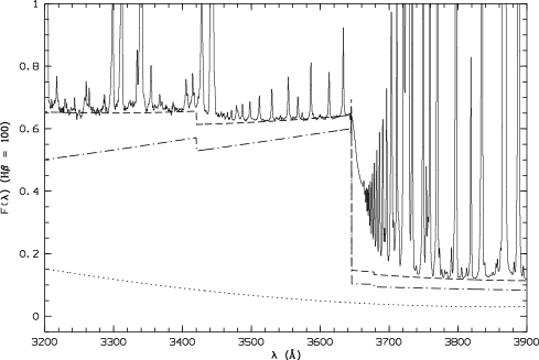
Figure 11: CCD spectrum (solid line) of NGC 7009 from 3200 to 3900 Å, showing the He i discontinuity at 3421 Å, as well as the Balmer discontinuity at 3646 Å. The intensity is normalized such that H$\beta$ = 100, and corrected for extinction. The dashed line is the total continuum, the sum of the theoretical nebular continuum (dot-dashed line) and the scattered stellar light (dotted line).

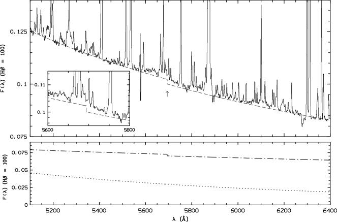
Figure 12: $Upper~{}Panel$: CCD spectrum of NGC 7009 (solid line) from 5100 to 6400 Å, showing the He ii discontinuity at 5694 Å  marked by an arrow. The insert is a zoom of the jump. The dashed line is a fit to the continuum level of the spectrum. $Lower~{}Panel$: The theoretical nebular continuum (dot-dashed line) and scattered stellar light (dotted line). The lower panel is not on the same scale as the upper one.

5 Discussion

5.1 Flux errors

The spectrum of NGC 7009 presented in the current work is among the deepest CCD spectra ever taken for an emission line nebula. The high S/N’s coupled with the medium resolution make it difficult to find a line-free region to estimate the local continuum and its uncertainties, and consequently the uncertainties of the fluxes of individual emission lines. Here we have adopted the flux errors yielded by the multi-Gaussian fitting, and they are listed in the last column of Table LABEL:linelist.

The errors vary but only have a weak dependence on wavelength. They do have a strong dependence on the strength of the line, as expected. Table 4 shows the average flux errors for different flux bins. Also presented in Table 4 are the numbers of the emission lines in each flux bins. For lines with fluxes higher than $\log[F(\lambda)/F({\rm H}\beta)]>-5.0$, those with flux errors larger than 100$\%$ are excluded in the calculation of the average error of individual flux bin, and their numbers are given in the notes to Table 4.

Amongst the large number of lines detected or deblended in the spectrum of NGC 7009, of particular interests are ORLs from C ii, N ii, O ii and Ne ii, and they will be analyzed separately in a subsequent paper. Those ORLs have typical fluxes about 10^-4 to 10^-2 of H$\beta$, with typical measurement uncertainties of 10 to 20 per cent (Table 4). The best observed ORLs of N ii and O ii have errors that are well below 10 per cent: e.g., the fitted intensity of O ii M1 3p ⁴D${}^{\rm o}_{7/2}$ – 3s ⁴P_5/2 $\lambda$4649.13, which is shown in Fig. 2, is 0.666 (on a scale where H$\beta$ is 100), with a fitting error of less than 2 per cent; the fitted intensity of N ii M3 3p ³D₃ – 3s ³P${}^{\rm o}_{2}$ $\lambda$5679.56 is 0.136 (H$\beta$ = 100), and its fitting error is about 5 per cent. The Ne ii M2 3p ⁴D${}^{\rm o}_{7/2}$ – 3s ⁴P_5/2 $\lambda$3334.84 line has a measured intensity of 0.428 (H$\beta$ = 100), with a fitting error of 8 per cent. Accurate measurements of those ORLs are of paramount importance for plasma diagnostics and abundance determinations using ORLs.

Table 4: Flux measurement errors.

Flux range	Number	The average	Note
	of lines	error (%)
$-$5.0 $<$ $\log[F(\lambda)/F({\rm H}\beta)]$ $<$ $-$4.0	312	$>$28.0	(1)
$-$4.0 $<$ $\log[F(\lambda)/F({\rm H}\beta)]$ $<$ $-$3.0	627	19.3	(2)
$-$3.0 $<$ $\log[F(\lambda)/F({\rm H}\beta)]$ $<$ $-$2.0	157	10.6	(3)
$-$2.0 $<$ $\log[F(\lambda)/F({\rm H}\beta)]$ $<$ $-$1.0	64	6.34	(4)
$-$1.0 $<$ $\log[F(\lambda)/F({\rm H}\beta)]$ $<$ 0	15	1.56
0 $<$ $\log[F(\lambda)/F({\rm H}\beta)]$ $<$ 2.0	5	$<$0.1

(1)

93 lines with errors larger than 100%.

(2)

28 lines with errors larger than 100%.

(3)

2 lines with errors larger than 100%.

(4)

2 lines with errors larger than 100%.

5.2 Number of lines

5.2.1 Cumulative numbers

The current spectrum is among the deepest ever taken for a PN, which allows the detection or deblending of many weak ORLs that are valuable for nebular analyses. In this subsection, a statistical analysis of the distribution of the emission lines as a function of intensity is presented. Fig. 13 shows the cumulative numbers of lines exceeding a given flux level relative to H$\beta$. For comparison, also shown in the Figure are numbers of emission lines detected in deep spectroscopy of a number of PNe published in the recent literature: NGC 7027 (short-dashed curve, labeled with number 2; Zhang et al. 2005a ), IC 418 (dot-dashed curve, labeled with number 3; Sharpee et al. sharpee2003 2003), IC 2501 (long-dashed curve, labeled with number 4; Sharpee et al. sharpee2007 2007), IC 4191 (dot-dot-dashed curve, labeled with number 5; Sharpee et al. sharpee2007 2007), NGC 2440 (dotted curve, labeled with number 6; Sharpee et al. sharpee2007 2007). In Fig. 13, for curves labeled by the numbers from 1 to 6, we consider only those lines within the wavelength range 3510 – 7470 Å which is covered by all the spectra. The curve of cumulative number of lines measured in NGC 7009 over the whole wavelength range 3040 – 11,000 Å is also presented (the dotted curve, which is labeled by 0).

In the wavelength range 3510 – 7470 Å, for the very weak intensity bin ($-5.0\leq\log[F(\lambda)/F({\rm H}\beta)]\leq-4.0$), 270 lines are measured and identified in NGC 7009, 251 in NGC 7027 (Zhang et al. 2005a ), 418 in IC 418 (Sharpee et al. sharpee2003 2003) and 421, 299 and 166 respectively in the remaining three PNe, IC 2501, IC 4191 and NGC 2440 (Sharpee et al. sharpee2007 2007). In the same wavelength range, for the medium weak intensity bin ($-4.0\leq\log[F(\lambda)/F({\rm H}\beta)]\leq-3.0$), NGC 7009 yields 459 lines identified, NGC 7027 311, IC 418 204 and the other three PNe, IC 2501, IC 4191 and NGC 2440 215, 286 and 230, respectively. In the weak to strong intensity bin ($\log[F(\lambda)/F({\rm H}\beta)]>-3.0$), NGC 7009 gives 153 lines, NGC 7027 158, IC 418 105 and the other three PNe, IC 2501, IC 4191 and NGC 2440 110, 143 and 175, respectively.

In Fig. 13, all curves start to flatten out at $\log[F(\lambda)/F({\rm H}\beta)]\sim-4.6$, where the line detection incompleteness kicks in, even though lines continue to be detected at fainter intensities. In the case of NGC 7009, no lines are detected with reliable identifications with logarithmic intensities lower than $-5.0$. The detection limit of the current spectrum of NGC 7009 is similar to that of NGC 7027 (Zhang et al. 2005a ) but is obviously lower than the deepest echelle spectrum ever taken for a PN, i.e. that of IC 2501 (Sharpee et al. sharpee2007 2007).

In the wavelength range 3510 – 7470 Å, the total number of emission lines identified in NGC 7009 is 887, larger than in all other PNe shown in Fig. 13, including NGC 7027 (684 lines), NGC 2440 (572 lines), IC 418 (732 lines), IC 4191 (778 lines) and IC 2501 (833 lines). That is because many optical recombination lines are taken into account and are deblended from the spectra of NGC 7009, although our resolution is much lower than those echelle spectra. The total number of the emission lines of NGC 7009, in the complete wavelength range 3040 – 11,000 Å, is more than 1300, as is shown in Fig. 13. The 235 alternative identifications given by emili are excluded from the calculation of the cumulative line numbers.

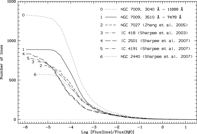
Figure 13: Cumulative number of emission lines exceeding a given flux level identified in the spectrum of NGC 7009 and in several recently published deep spectra of other PNe. For the curves labeled with numbers 1, 2, 3, 4, 5 and 6, we consider only lines within the wavelength range 3510 – 7470 Å, which is the common range covered by the observations of these PNe. For curve 1, the dubious identifications in NGC 7009 are not included. The dotted curve 0 includes all emission lines of NGC 7009 in the whole wavelength range from 3040 to 11,000 Å, except those 235 alternative identifications given by emili.

5.2.2 Emission lines from different ionic species

In Table 5 we summarize for each ionic species the number of permitted lines identified in NGC 7009. In total 986 permitted lines are identified, and most of them are excited mainly by recombination. Similar results for forbidden lines (CELs) are presented in Table 6. These include a total of 234 lines. Dubious identifications are excluded from both tables.

Nearly 200 O ii permitted lines are identified in NGC 7009. In addition, more than 100 N ii and Ne ii lines are identified. The identifications of a few Ne ii lines, those from very high-$n$, with $n\,\geq\,7$, may be problematic. Further observations are needed to establish their legitimacy. Only 34 C ii permitted lines are identified. The relatively small number of C ii lines is due to the relatively simple atomic structure, i.e., an ion with only one valence electron.

Several permitted lines emitted by highly ionized species of the most abundant heavy elements (C and O) are also detected or deblended in the spectrum of NGC 7009: For example, C iv M8 6h ²H^o – 5g ²G $\lambda$4658 (please see Fig. 2) and O iv M2 3d ²D – 3p ²P^o $\lambda$3409. Here the C iv $\lambda$4658 line may contain a small contamination from the [Fe iii] $\lambda$4658 line (Liu et al. liu1995 1995).

Table 5: Numbers of permitted lines identified for all ionic species. Lines with dubious identifications are not included.

Ion	No. of	Note
	lines
H i	60
He i	93
He ii	65
C i	13
C ii	34
C iii	25
C iv	3
N i	11
N ii	117
N iii	36
O i	17
O ii	192
O iii	47
O iv	3
Ne i	10
Ne ii	135
Ne iii	1
Na i	3
Mg i	5
Mg i$]$	3
Mg ii	2
Al ii	1
Si i	3
Si ii	13
Si iii	12
Si iv	5
S ii	2
Ar i	3
Ar ii	5
Ca i	2
Fe i	4
Fe ii	48
Fe iii	11

Table 6: Same as Table 5, but for CELs.

Ion	No. of	Note
	lines
$[$C i$]$	2
$[$N i$]$	2
$[$N ii$]$	4
$[$O i$]$	3
$[$O ii$]$	4
$[$O iii$]$	4
$[$F ii$]$	1
$[$F iv$]$	1
$[$Ne iii$]$	4
$[$Ne iv$]$	4
$[$P ii$]$	1	(1)
$[$S ii$]$	4
$[$S iii$]$	4
$[$Cl ii$]$	3
$[$Cl iii$]$	4
$[$Cl iv$]$	3
$[$Ar iii$]$	4
$[$Ar iv$]$	4
$[$Ar v$]$	2
$[$K iv$]$	2
$[$K v$]$	1
$[$K vi$]$	1
$[$Ca v$]$	1
$[$V ii$]$	6
$[$Cr ii$]$	6
$[$Cr iii$]$	6
$[$Cr iv$]$	4
$[$Cr v$]$	3
$[$Mn ii$]$	1
$[$Mn iii$]$	1
$[$Mn v$]$	14
$[$Mn vi$]$	2
$[$Fe ii$]$	56
$[$Fe iii$]$	25
$[$Fe iv$]$	15
$[$Fe v$]$	8
$[$Fe vi$]$	8
$[$Fe vii$]$	1
$[$Co ii$]$	1
$[$Co iii$]$	2
$[$Co iv$]$	1
$[$Co v$]$	1
$[$Ni ii$]$	5
$[$Ni iii$]$	2
$[$Ni iv$]$	3

(1)

Blended with O ii M89b 4f D[2]${}^{\rm o}_{5/2}$ – 3d ²D_3/2 $\lambda$4669.27, which contributes about 40 per cent to the blend at $\lambda$4669.

Fig. 14 shows the histograms of intensity distributions of all the lines identified, as well as those of permitted lines from the most prominent heavy element ions, C ii, N ii, O ii and Ne ii. Fig. 15 shows the distributions of the strengths of all identified ORLs and CELs. Most ORLs as well as CELs have intensities between 10^-5 and 10^-2 of H$\beta$.

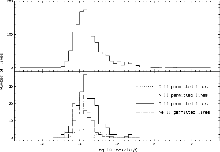
Figure 14: $Upper~{}panel$: Histograms showing the intensity distributions of all lines identified. $Lower~{}panel$: Histograms showing the distributions of C ii, N ii, O ii and Ne ii permitted lines. Lines with dubious identifications are not counted.

Figure 15: Histograms showing the intensity distributions of ORLs and CELs in NGC 7009. Lines with dubious identifications are not counted.

6 Summary

Based on very deep, medium-resolution long-slit spectra of the Saturn Nebula NGC 7009, we have detected, deblended and estimated more than 1400 emission lines, with the weakest lines estimated down to intensity levels from 10^-6 to 10^-5 that of H$\beta$. In total 1170 emission lines are identified, both manually and systematically by the computer-aided code emili. Multi-Gaussian line profile fitting is carried out across the whole wavelength range (3040 – 11,000 Å) to retrieve intensities of blended features. We first manually identify all the obvious emission features in the spectra, following the traditional method. Then we use multi-Gaussian fitting to obtain fluxes of weak lines that are blended with strong features. The most updated atomic transition data are utilized to estimate the fluxes of those weak lines whose reliable measurements are difficult. Finally, all the aforementioned features, except those that are simply estimated from atomic data, are further identified with emili. All the emission lines are presented in a comprehensive table with all detailed transition information included.

In addition to singly and doubly ionized species, recombination lines emitted by highly ionized ions of C, N and O are also identified. We also detected forbidden lines from neutral species C i, N i and O i. The majority of lines are in the flux range 10^-5 – 10^-2 that of H$\beta$.

Compared to several other PNe that have been extensively studied in the recent literature, NGC 7009 exhibits much more faint emission lines, thanks to its very rich and prominent ORL spectra from abundant second-row elements. The current set of spectra of NGC 7009 are among the deepest ever taken for a PN. The detection limit of the current data set is limited by the relatively low spectral resolution. Spectroscopy of this bright PN with better resolution will no doubt lead to direct detection of more and fainter lines.

Figure 16: Continued.

Figure 16: Continued.

Figure 16: Continued.

Figure 16: Continued.

Figure 16: Continued.

Figure 16: Continued.

Figure 16: Continued.

Figure 16: Continued.

Figure 16: Continued.

Figure 16: Continued.

Figure 16: Continued.

Table 7: Emission line list of NGC 7009. The line fluxes are normalized such that H$\beta$ = 100.

$\lambda_{\mathrm{obs}}$(Å)	$F(\lambda)$	$I(\lambda)$		ID	$\lambda_{\mathrm{lab}}$(Å)	Mul.	Lower Term	Upper Term	$g_{1}$	$g_{2}$	Error (%)
3041.49	0.2480	0.3170		Si II	3042.19	V14	3d’ 4D*	4f’ 4D	8	8	:
			*	Si II	3042.18	V14	3d’ 4D*	4f’ 4D	4	4
3043.75	1.3100	1.6737		Ne III	3044.24		3s 3D*	3p 3D	3	5	5.75
			*	Ne II	3045.56	V8	3p 4P*	3d 4D	2	2
3045.50	3.7120	4.7410		O III	3047.12	V4	3s 3P*	3p 3P	5	5	3.03
3046.82	0.0950	0.1213		Ne II	3047.56	V8	3p 4P*	3d 4D	4	6	86.32
3058.27	1.0840	1.3814		O III	3059.30	V4	3s 3P*	3p 3P	5	3	7.56
			*	C V	3057.50		3s 3S	3p 3P*	3	5
			*	Ne II	3057.83		3d 2F	5f 0$<$3$>$*	6	6
			*	Ne II	3057.87		3d 2F	5f 0$<$3$>$*	6	8
3060.68	0.1220	0.1554		[Cr III]	3061.49		3d4 1F	3d4 1G	7	9	37.46
3107.84	0.1420	0.1794		[Ar III]	3109.17		3p4 3P	3p4 1S	3	1	35.21
3114.71	0.0870	0.1098		O III	3115.68	V12	3p 3S	3d 3P*	3	1	34.48
			*	Fe II	3115.35	V121	c2G	z2H*	10	10
3120.49	1.1510	1.4515		O III	3121.64	V12	3p 3S	3d 3P*	3	3	4.34
			*	Fe I	3121.15	V163	z7D	g5D	3	5
3124.33	0.0400	0.0504		Ne II	3124.95		3d’ 2F	5f’2$<$3$>$*	6	6	:
			*	Ne II	3124.98		3d’ 2F	5f’2$<$3$>$*	8	8
3131.70	29.9830	37.7420		O III	3132.79	V12	3p 3S	3d 3P*	3	5	6.67
3137.60	0.0430	0.0541		Ne II	3138.13		3d 4F	5f 2$<$2$>$*	4	4	34.88
3148.23	0.0350	0.0439		Ne II	3149.09		3d 2F	5f 2$<$3$>$*	6	8	57.14
			*	Ne II	3149.04		3d 2F	5f 2$<$3$>$*	6	6
3161.95	0.0540	0.0677		C II	3162.66		4f 2F*	5d 2D	6	6	27.78
3164.87	0.0800	0.1002		C II	3165.47	V9	2p3 2D*	3p’ 2P	6	4	25.00
			*	C II	3165.97	V9	2p3 2D*	3p’ 2P	4	4
3168.56	0.0580	0.0726		He I	3169.02		2s 1S	15p 1P*	1	3	25.86
3175.37	0.0290	0.0363		He I	3176.27		2s 1S	14p 1P*	1	3	24.14
3186.79	2.8410	3.5457		He I	3187.74	V3	2s 3S	4p 3P*	3	9	9.86
3194.37	0.0320	0.0399		?							31.25
			*	Ne II	3198.92	V13	3p 4D*	3d 4F	4	4
3202.24	4.8092	5.9883		He II	3203.17	3.5a	3d 2D	5f 2F*	6	8	9.66
3209.95	0.0710	0.0883		[Fe II]	3210.74		a6D	b2F	4	8	21.13
3214.07	0.0670	0.0833		[Fe II]	3214.67		(5D)4s 6D	(3D)4s 4D	8	8	20.90
3217.25	0.1880	0.2336		Ne II	3218.19	V13	3p 4D*	3d 4F	8	10	9.95
3228.91	0.0580	0.0719		Si II	3229.55		3d’ 2P*	4f’ 2D	4	6	10.34
3229.87	0.0560	0.0694		N II	3230.54		3D	3P*	7	5	10.71
3231.56	0.0500	0.0620		?							12.00
3243.22	0.0600	0.0743		Ne II	3244.09	V13	3p 4D*	3d 4F	6	8	10.00
3250.23	0.0210	0.0260		Fe III	3250.84		4G 4d3I	2I 5p3I*	11	11	42.38
3257.97	0.0670	0.0828		[Mn II]	3258.56		a7S	a3H	7	11	15.82
3260.14	0.1490	0.1840		O III	3260.85	V8	3p 3D	3d 3F*	5	7	8.86
3264.61	0.1160	0.1432		O III	3265.32	V8	3p 3D	3d 3F*	7	9	9.48
3266.49	0.0170	0.0210		O III	3267.20	V8	3p 3D	3d 3F*	3	5	52.35
3276.61	0.0120	0.0148		Fe II]	3277.35	V1	a4D	z6D*	8	10	74.17
3286.78	0.0850	0.1046		[Fe II]	3287.35		a6D	b4D	2	6	12.35
3289.46	0.0220	0.0271		O II	3289.98	V23	3p 4P*	4s 4P	2	4	40.91
3298.64	1.1070	1.3598		O III	3299.40	V3	3s 3P*	3p 3S	1	3	9.79
			*	Ne II	3297.73	V2	3s 4P	3p 4D*	6	6
3303.62	0.0390	0.0479		Fe III	3304.31		2S 4s3S	4D 4p3P*	3	5	:
3311.61	3.0740	3.7695		O III	3312.32	V3	3s 3P*	3p 3S	3	3	5.57
			*	Ne II	3311.27	V2	3s 4P	3p 4D*	4	2
3321.71	0.0480	0.0588		[Fe III]	3322.53		5D	7S	9	7	:
3323.74	0.0600	0.0735		Cr II	3324.47		x6D*	5D 9s6D	8	10	66.67
3325.94	0.0460	0.0563		Ne II	3327.15	V2	3s 4P	3p 4D*	4	4	29.13
3328.47	0.0430	0.0526		Ne II	3329.16	V12	3p 4D*	3d 4D	8	8	31.40
3330.04	0.0120	0.0147		Ne II	3330.73	V20	3p 2D*	3d 2F	6	6	:
3331.31	0.0610	0.0746		[Fe II]	3331.96		a6D	b2G	8	10	45.90
3334.16	0.3500	0.4279		Ne II	3334.84	V2	3s 4P	3p 4D*	6	8	8.46
3340.07	4.4230	5.4035		O III	3340.76	V3	3s 3P*	3p 3S	5	3	6.50
3341.68	0.6390	0.7805		[Ne III]	3342.50		2p4 1D	2p4 1S	5	1	1.96
			*	Ne II	3344.40	V2	3s 4P	3p 4D*	2	2
3345.08	0.0110	0.0134		Ne II	3345.88	V12	3p 4D*	3d 4D	6	4	36.36
3350.05	0.0360	0.0439		Fe I	3350.62		z5P*	7/2$<$3/2$>$	3	5	27.78
3352.47	0.0650	0.0793		[Cl III]	3353.17		3p3 4S*	3p3 2P*	4	2	15.38
3353.90	0.1403	0.1711		He I	3354.55	V8	2s 1S	7p 1P*	1	3	6.37
3354.52	0.1827	0.2228		Ne II	3355.02	V2	3s 4P	3p 4D*	4	6	6.02
3357.07	0.0170	0.0207		Ne II	3357.82	V12	3p 4D*	3d 4D	6	6	58.82
3359.95	0.0330	0.0402		Ne II	3360.60	V2	3s 4P	3p 4D*	1	3	30.30
			*	O II	3360.62	V52	3d 4F	5p 4D*	4	6
3362.11	0.0220	0.0268		Ne II	3362.94	V12	3p 4D*	3d 4D	4	2	45.45
			*	Ne II	3362.71	V42	3p 2P*	4s 2P	4	2
3366.73	0.0870	0.1059		Ne II	3367.22	V20	3p 2D*	3d 2F	6	8	11.49
			*	Ne II	3366.98	V12	3p 4D*	3d 4D	6	8
			*	N III	3367.36	V5	3s’ 4P*	3p’ 4P	6	6
3370.30	0.0490	0.0596		Co II	3370.92	V2	a5P	z5D*	3	1	20.41
3373.30	0.0120	0.0146		Ne II	3374.06	V12	3p 4D*	3d 4D	4	4	83.33
3373.67	0.0170	0.0207		?							58.82
3377.33	0.0240	0.0292		?							41.67
			*	Ne II	3379.32	V12	3p 4D*	3d 4D	2	2
3386.35	0.0450	0.0547		[Fe II]	3387.09		a4F	b4D	10	6	22.22
			*	Ne II	3386.20	V12	3p 4D*	3d 4D	4	6
3389.85	0.0140	0.0170		Ne II	3390.55	V12	3p 4D*	3d 4D	2	4	71.43
3392.12	0.0090	0.0109		Ne II	3393.18	V21	3p 2D*	3d 2D	6	4	:
3402.91	0.0490	0.0594		O IV	3403.52	V2	3p 2P*	3d 2D	2	4	20.41
3405.11	0.1630	0.1975		O III	3405.71	V15	3p 3P	3d 3P*	1	3	6.13
3407.12	0.0860	0.1042		O III	3408.12	V15	3p 3P	3d 3P*	3	1	11.63
3411.08	0.0400	0.0484		O IV	3411.69	V2	3p 2P*	3d 2D	4	6	25.00
3413.03	0.0450	0.0545		O IV	3413.64	V2	3p 2P*	3d 2D	4	4	22.22
3414.61	0.3430	0.4152		O III	3415.26	V15	3p 3P	3d 3P*	3	3	2.92
3416.27	0.0640	0.0775		Ne II	3416.91	V21	3p 2D*	3d 2D	6	6	15.62
3417.05	0.0300	0.0363		Ne II	3417.69	V19	3p 2D*	3d 4F	6	8	33.33
3422.86	0.0770	0.0931		Ne I	3423.91	V2.4	3s 2$<$2$>$*	4p 1$<$2$>$	3	3	12.99
3427.92	1.1660	1.4091		O III	3428.62	V15	3p 3P	3d 3P*	3	5	0.86
			*	O II	3428.51		3d 4P	5p 4S*	6	4
3429.87	0.2640	0.3190		O III	3430.57	V15	3p 3P	3d 3P*	5	3	3.79
			*	He I	3430.56		2p 3P*	35s 3S	1	3
3433.94	0.0170	0.0205		He I	3434.68		2p 3P*	31s 3S			58.82
3443.33	9.5950	11.5747		O III	3444.06	V15	3p 3P	3d 3P*	5	5	2.57
3446.76	0.1680	0.2026		He I	3447.59	V7	2s 1S	6p 1P*	1	3	2.86
3449.81	0.0180	0.0217		He I	3450.28		2p 3P*	21d 3D	9	15	55.56
			*	O III	3450.92	V25	3p’ 5D*	3d’ 5F	7	9
3452.69	0.0160	0.0193		He I	3453.32		2p 3P*	20d 3D	9	15	62.50
			*	Ne II	3453.07	V21	3p 2D*	3d 2D	4	4
3456.09	0.0295	0.0355		He I	3456.86		2p 3P*	19d 3D	9	15	33.33
			*	Ne II	3456.61	V28	3p 2S*	3d 2P	2	4
3459.92	0.0320	0.0385		He I	3461.01		2p 3P*	18d 3D	9	15	31.25
3463.15	0.0140	0.0168		N III	3463.74		2D	2F*	6	6	71.43
3465.25	0.0360	0.0433		He I	3465.94	V45	2p 3P*	17d 2D	9	15	27.78
			*	O III	3466.11	V25	3p’ 5D*	3d’ 5F	9	9
3470.97	0.0510	0.0613		He I	3471.81	V44	2p 3P*	16d 3D	9	15	19.61
3476.93	0.0100	0.0120		Ne II	3477.65	V21	3p 2D*	3d 2D	4	6	30.00
			*	N IV	3478.71	V1	3s 3S	3p 3P*	3	5
3478.27	0.0730	0.0877		He I	3478.97	V43	2p 3P*	15d 3D	9	15	13.70
3479.78	0.0450	0.0541		O II	3480.25		3d 4P	5p 4P*	4	4	22.22
			*	[Fe III]	3480.57		3F4	3F2	9	5
3481.21	0.0362	0.0434		Ne II	3481.93	V6	3s 2P	3p 2S*	4	2	33.33
			*	[Fe III]	3481.82		3F4	3P2	7	5
			*	N IV	3482.99	V1	3s 3S	3p 3P*	3	3
3486.99	0.0850	0.1020		He I	3487.72	V42	2p 3P*	14d 3D	9	15	9.41
3495.16	0.0180	0.0216		[Fe III]	3496.08		3F4	3F2	7	7	27.78
3497.82	0.1030	0.1235		He I	3498.64	V40	2p 3P*	13d 3D	9	15	7.77
3502.42	0.0100	0.0120		Ne II	3503.58	V28	3p 2S*	3d 2P	2	2	50.00
3511.64	0.1340	0.1604		He I	3512.51	V38	2p 3P*	12d 3D	9	15	5.97
3526.70	0.0100	0.0120		Ne II	3527.36		2F*	2F	8	8	50.00
3529.70	0.1590	0.1899		He I	3530.49	V36	2p 3P*	11d 3D	9	15	3.14
3536.21	0.0190	0.0227		He I	3536.94		2p 3P*	11s 3S	9	3	26.32
			*	Ne II	3537.00		3d 2D	5p 2P*	4	4
3539.65	0.0110	0.0131		Ni I	3540.33	V119	z5F*	i3F	3	5	45.45
3542.01	0.0260	0.0310		Ne II	3542.85	V34	3p 4S*	3d 4P	4	6	19.23
3544.56	0.0160	0.0191		?							31.25
3549.78	0.0160	0.0191		Si III	3550.38	V8.01	3d’ 3F*	5d 3D	5	3	31.25
3553.60	0.2220	0.2645		He I	3554.41	V34	2p 3P*	10d 3D	9	15	2.25
3557.00	0.0120	0.0143		Ne II	3557.81	V6	3s 2P	3p 2S*	2	2	41.67
3562.01	0.0240	0.0286		He I	3562.95	V33	2p 3P*	10s 3S	9	3	22.50
3564.83	0.0210	0.0250		Ne II	3565.82	V34	3p 4S*	3d 4P	4	4	26.67
3567.62	0.1410	0.1678		Ne II	3568.50	V9	3s’ 2D	3p’ 2F*	6	8	9.93
3573.68	0.0450	0.0535		Ne II	3574.18	V9	3s’ 2D	3p’ 2F*	6	6	4.67
			*	Ne II	3574.61	V9	3s’ 2D	3p’ 2F*	4	6
3577.71	0.0050	0.0059		Fe I	3578.55		a3G	n7P*	7	9	:
3580.06	0.0050	0.0059		C III	3580.68		3G	3G*	7	11	:
3586.43	0.2920	0.3467		He I	3587.27	V31	2p 3P*	9d 3D	9	15	1.71
3589.55	0.0320	0.0380		Ne II	3590.45	V31	3p 4S*	3d 4F	4	6	15.62
			*	C I	3590.21	V7.08	3s 3P*	7p 3P	3	5
3593.58	0.0100	0.0119		Ne II	3594.16	V34	3p 4S*	3d 4P	4	2	50.00
3598.29	0.0200	0.0237		He I	3599.32	V30	2p 3P*	9s 3S	9	3	14.50
3600.16	0.0220	0.0261		?							13.64
3602.58	0.0120	0.0142		Ne II	3603.24		3d 4D	5p 4P*	4	4	18.33
3612.77	0.2440	0.2890		He I	3613.64	V6	2s 1S	5p 1P*	1	3	4.30
3633.36	0.4530	0.5354		He I	3634.23	V28	2p 3P*	8d 3D	9	15	3.18
3643.10	0.0160	0.0189		Ne II	3643.93	V5	3s 2P	3p 2D*	4	4	12.50
3647.12	0.0180	0.0212		[Fe II]	3647.78		a4D	b2D	2	6	11.11
3650.87	0.0140	0.0165		H I	3651.82	H50	2p+ 2P*	50d+ 2D	8		35.71
			*	He I	3652.00	V27	2p 3P*	8s 3S	9	3
3663.65	0.0760	0.0893		H I	3664.68	H28	2p+ 2P*	28d+ 2D	8		6.58
			*	Ne II	3664.07	V1	3s 4P	3p 4P*	6	4
3665.24	0.1360	0.1598		H I	3666.09	H27	2p+ 2P*	27d+ 2D	8		7.35
3666.89	0.1930	0.2267		H I	3667.68	H26	2p+ 2P*	26d+ 2D	8		5.18
3668.63	0.2210	0.2596		H I	3669.46	H25	2p+ 2P*	25d+ 2D	8		4.52
3670.59	0.3530	0.4144		H I	3671.48	H24	2p+ 2P*	24d+ 2D	8		40.23
3672.95	0.4180	0.4905		H I	3673.76	H23	2p+ 2P*	23d+ 2D	8		34.86
3675.50	0.5050	0.5924		H I	3676.36	H22	2p+ 2P*	22d+ 2D	8		16.22
3678.51	0.5570	0.6530		H I	3679.35	H21	2p+ 2P*	21d+ 2D	8		11.92
3681.97	0.6220	0.7287		H I	3682.81	H20	2p+ 2P*	20d+ 2D	8		5.98
3685.99	0.7120	0.8336		H I	3686.83	H19	2p+ 2P*	19d+ 2D	8		1.10
3690.71	0.7780	0.9100		H I	3691.55	H18	2p+ 2P*	18d+ 2D	8		5.27
3693.42	0.2170	0.2537		Ne II	3694.21	V1	3s 4P	3p 4P*	6	6	10.14
3696.29	0.9310	1.0879		H I	3697.15	H17	2p+ 2P*	17d+ 2D	8		4.68
3701.08	0.2550	0.2977		Ne II	3701.78	V40	3p 2P*	3d 4P	4	6	9.96
			*	O III	3702.75	V14	3p 3P	3d 3D*	1	3
3702.90	1.3020	1.5196		H I	3703.85	H16	2p+ 2P*	16d+ 2D	8		2.91
3704.20	0.7640	0.8915		He I	3705.00	V25	2p 3P*	7d 3D	9	15	6.06
3706.49	0.2860	0.3336		O III	3707.25	V14	3p 3P	3d 3D*	3	5	7.45
			*	He I	3707.34		2p 1P*	23s 1S	3	1
3708.82	0.0940	0.1096		Ne II	3709.62	V1	3s 4P	3p 4P*	4	2	23.09
			*	He I	3709.65		2p 1P*	22d 1D	3	5
3711.17	1.3790	1.6071		H I	3711.97	H15	2p+ 2P*	15d+ 2D	8		2.89
			*	He I	3712.70		2p 1P*	21d 1D	3	5
			*	O II	3712.74	V3	3s 4P	3p 4S*	4	4
3712.28	0.2630	0.3064		Ne II	3713.08	V5	3s 2P	3p 2D*	4	6	9.51
			*	O III	3714.03	V14	3p 3P	3d 3D*	3	3
3714.32	0.2350	0.2737		O III	3715.08	V14	3p 3P	3d 3D*	5	7	13.74
3714.40	0.0210	0.0245		He II	3715.16	4.29	4f+ 2F*	29g+ 2G	32		47.62
			*	He I	3716.22		2p 1P*	20d 1D	3	5
			*	Cr II	3715.19	V20	b4D	z4F*	8	10
3719.70	0.0150	0.0175		He II	3720.41	4.28	4f+ 2F*	28g+ 2G	32		33.33
3720.98	0.9280	1.0796		[S III]	3721.69	F2	3p2 3P	3p2 1S	3	1	2.16
3721.23	2.5410	2.9560		H I	3721.94	H14	2p+ 2P*	14d+ 2D	8		2.22
			*	O III	3725.31	V14	3p 3P	3d 3D*	5	5
3725.17	11.8090	13.7280		[O II]	3726.03	F1	2p3 4S*	2p3 2D*	4	4	0.17
3725.56	0.0170	0.0198		He II	3726.27	4.27	4f+ 2F*	27g+ 2G	32		29.41
			*	Ne II	3727.11	V5	3s 2P	3p 2D*	2	4
3727.92	5.9400	6.9019		[O II]	3728.81	F1	2p3 4S*	2p3 2D*	4	6	0.34
			*	O III	3732.12	V14	3p 3P	3d 3D*	5	3
3732.12	0.0180	0.0209		He II	3732.83	4.26	4f+ 2F*	26g+ 2G	32		27.78
3732.17	0.0290	0.0337		He I	3732.88	V24	2p 3P*	7s 3S	9	3	17.24
3733.55	1.9220	2.2310		H I	3734.37	H13	2p+ 2P*	13d+ 2D	8		1.75
			*	Ne II	3734.94	V1	3s 4P	3p 4P*	4	4
3739.32	0.0450	0.0522		O II	3739.76	V31	3p 4S*	4s 4P	4	6	11.11
3739.52	0.0210	0.0244		He II	3740.23	4.25	4f+ 2F*	25g+ 2G	32		47.62
3747.78	0.0210	0.0243		He II	3748.61	4.24	4f+ 2F*	24g+ 2G	32		23.81
3749.32	2.4810	2.8719		H I	3750.15	H12	2p+ 2P*	12d+ 2D	8		2.55
			*	Ne II	3751.25	V1	3s 4P	3p 4P*	2	2
3753.94	0.5688	0.6579		O III	3754.70	V2	3s 3P*	3p 3D	3	5	5.46
			*	He I	3756.10	V66	2p 1P*	14d 1D	3	5
3756.43	0.3091	0.3574		O III	3757.24	V2	3s 3P*	3p 3D	1	3	20.13
			*	He II	3758.15	4.23	4f+ 2F*	23g+ 2G	32		41.67
3759.09	1.5782	1.8238		O III	3759.87	V2	3s 3P*	3p 3D	5	7	2.97
3761.36	0.0810	0.0936		Mg I	3762.10		1D	1P*	5	3	12.35
			*	Ne II	3766.26	V1	3s 4P	3p 4P*	4	6
3768.02	0.0280	0.0323		He I	3768.81	V65	2p 1P*	13d 1D	3	5	2.14
3768.29	0.0260	0.0300		He II	3769.08	4.22	4f+ 2F*	22g+ 2G	32		2.31
3769.84	3.2770	3.7797		H I	3770.63	H11	2p+ 2P*	11d+ 2D	8		2.17
3773.12	0.1670	0.1925		O III	3774.02	V2	3s 3P*	3p 3D	3	3	32.16
3776.37	0.0430	0.0495		Ne II	3777.14	V1	3s 4P	3p 4P*	2	4	23.26
3780.89	0.0380	0.0437		He II	3781.68	4.21	4f+ 2F*	21g+ 2G	32		26.32
3783.92	0.0320	0.0368		He I	3784.86	V64	2p 1P*	12d 1D	3	5	31.25
3790.52	0.1554	0.1786		O III	3791.28	V2	3s 3P*	3p 3D	5	5	20.62
3795.55	0.4280	0.4915		He II	3796.33	4.20	4f+ 2F*	20g+ 2G	32		11.12
3797.12	4.3400	4.9824		H I	3797.90	H10	2p+ 2P*	10d+ 2D	8		1.63
3801.49	0.0050	0.0057		Ne II	3802.29		4d 4D	4f’2$<$1$>$*	6	4	:
3805.00	0.0430	0.0493		He I	3805.74	V63	2p 1P*	11d 1D	3	5	23.26
3805.82	0.0200	0.0229		Si III	3806.54	V5	4p 3P*	4d 3D	10	12	50.00
			*	Si III	3806.78	V5	4p 3P*	4d 3D	5	3
3810.24	0.0100	0.0115		O III	3810.99	V2	3s 3P*	3p 3D	5	3	:
3812.74	0.0570	0.0653		He II	3813.49	4.19	4f+ 2F*	19g+ 2G	32		35.09
3818.86	1.1470	1.3119		He I	3819.60	V22	2p 3P*	6d 3D	9	15	4.84
3832.80	0.0640	0.0730		He I	3833.57	V62	2p 1P*	10d 1D	3	5	0.94
3833.03	0.0460	0.0525		He II	3833.80	4.18	4f+ 2F*	18g+ 2G	32		0.87
3834.61	6.6300	7.5634		H I	3835.38	H9	2p+ 2P*	9d+ 2D	8		0.93
3837.60	0.0020	0.0023		N II	3838.37	V30	3p 3P	4s 3P*	5	5	:
3838.63	0.0850	0.0969		[Fe V]	3839.27		3d4 5D	3d4 3F2	7	7	0.94
3841.41	0.0004	0.0005		N II	3842.18	V30	3p 3P	4s 3P*	1	3	:
3842.08	0.0140	0.0160		O II	3842.82	V12	3p 4D*	3d 4D	2	4	5.71
3847.16	0.0120	0.0137		O II	3847.89	V12	3p 4D*	3d 4D	2	2	5.00
3850.06	0.0030	0.0034		O II	3850.80	V12	3p 4D*	3d 4D	4	6	6.67
3850.29	0.0150	0.0171		O II	3851.03	V12	3p 4D*	3d 4D	4	4	6.00
3850.61	0.0070	0.0080		[Fe V]	3851.35		3d4 5D	3d4 3F2	7	5	65.71
3852.93	0.0070	0.0080		Si II	3853.66	V1	3p2 2D	4p 2P*	4	4	37.14
3855.28	0.0461	0.0524		Si II	3856.02	V1	3p2 2D	4p 2P*	6	4	7.45
3855.39	0.0119	0.0135		O II	3856.13	V12	3p 4D*	3d 4D	4	2	6.36
3857.40	0.0740	0.0841		He II	3858.07	4.17	4f+ 2F*	17g+ 2G	32		5.41
3862.18	0.0610	0.0693		Si II	3862.60	V1	3p2 2D	4p 2P*	4	2	8.20
			*	Ne II	3862.59		5g 2$<$4$>$	5f’2$<$4$>$*	8	10
			*	O II	3863.50	V12	3p 4D*	3d 4D	6	8
			*	O II	3864.43	V12	3p 4D*	3d 4D	6	6
			*	O II	3864.67	V12	3p 4D*	3d 4D	6	4
3867.96	104.4480	118.4975		[Ne III]	3868.76	F1	2p4 3P	2p4 1D	5	5	0.01
3877.30	0.0300	0.0340		He I	3878.18	V59	2p 1P*	9s 1S	3	1	6.67
3881.45	0.0470	0.0532		O II	3882.19	V12	3p 4D*	3d 4D	8	8	1.28
3881.51	0.0370	0.0419		?							1.08
3881.71	0.0050	0.0057		O II	3882.45	V11	3p 4D*	3d 4P	4	4	2.00
3882.39	0.0030	0.0034		O II	3883.13	V12	3p 4D*	3d 4D	8	6	3.33
3883.08	0.0290	0.0328		C III	3883.82	V15	4d 3D	5f 3F*	3	5	1.03
			*	C II	3883.82	V33	3d’ 4F*	4f’ 4G	10	8
3886.70	0.0640	0.0724		He II	3887.44	4.16	4f+ 2F*	16g+ 2G	32		1.25
3887.91	9.9670	11.2710		He I	3888.64	V2	2s 3S	3p 3P*	3	9	1.19
3888.31	8.5920	9.7155		H I	3889.05	H8	2p+ 2P*	8d+ 2D	8		1.19
3890.58	0.1620	0.1831		[Fe V]	3891.28		3d4 5D	3d4 3F2	9	9	6.17
3894.52	0.0490	0.0554		[Fe V]	3895.22		3d4 5D	3d4 3P2	7	5	20.41
3895.26	0.0390	0.0441		Fe II]	3896.10	V23	a2D	z4P*	4	6	25.64
3901.99	0.0100	0.0113		P II	3902.87		3d 3D*	5p 3D	7	5	50.00
			*	Fe III	3902.81		4G 4d5F	4D 5p5F*	11	11
3906.61	0.0090	0.0101		O II	3907.45	V11	3p 4D*	3d 4P	6	6	55.56
3906.90	0.0080	0.0090		[Cr III]	3907.74		b1G	1H	9	11	62.50
3911.06	0.0200	0.0225		O II	3911.96	V17	3s’ 2D	3p’ 2P*	6	4	25.00
3914.16	0.0030	0.0034		C III	3914.90		3P*	3D	5	3	:
3918.19	0.0140	0.0158		C II	3918.98	V4	3p 2P*	4s 2S	2	2	19.29
3918.50	0.0100	0.0113		O II	3919.29	V17	3s’ 2D	3p’ 2P*	4	2	28.00
			*	N II	3919.00	V17	3p 1P	3d 1P*	3	3
3919.90	0.0300	0.0338		C II	3920.69	V4	3p 2P*	4s 2S	4	2	3.33
3922.74	0.1060	0.1192		He II	3923.48	4.15	4f+ 2F*	15g+ 2G	32		2.55
3923.64	0.0120	0.0135		Si III	3924.47	V8.14	4f 1F*	5g 1G	7	9	15.83
3925.79	0.1170	0.1315		He I	3926.53	V58	2p 1P*	8d 1D	3	5	0.94
3925.81	0.0020	0.0022		O II	3926.58	V11	3p 4D*	3d 4P	8	6	55.00
3928.01	0.0130	0.0146		C II	3928.80		4P*	4D	2	2	6.92
3930.87	0.0050	0.0056		O II	3931.55		G$<$5$>$*	2$<$6$>$	10	12	28.00
3935.11	0.0100	0.0112		He I	3935.91	V57	2p 1P*	8s 1S	3	1	20.00
3941.45	0.0060	0.0067		Ar II	3942.28		3d” 2D	5f 2$<$4$>$*	6	8	33.33
3944.18	0.0230	0.0258		O II	3945.04	V6	3s 2P	3p 2P*	2	4	7.20
			*	C II	3945.00	V32	3d’ 4F*	4f’ 4F	4	4
			*	C II	3945.20	V32	3d’ 4F*	4f’ 4F	6	8
3947.28	0.0270	0.0302		O III	3948.01	V26.04	4p 3D	5s 3P*	3	5	7.41
			*	C II	3947.72	V32	3d’ 4F*	4f’ 4F	8	10
			*	C II	3948.33	V32	3d’ 4F*	4f’ 4F	8	8
3953.72	0.0270	0.0302		O II	3954.36	V6	3s 2P	3p 2P*	2	2	7.41
3960.77	0.0280	0.0313		O III	3961.57	V17	3p 1D	3d 1F*	5	7	17.86
3963.93	1.0640	1.1888		He I	3964.73	V5	2s 1S	4p 1P*	1	3	8.18
3966.67	30.4230	33.9772		[Ne III]	3967.47	F1	2p4 3P	2p4 1D	3	5	0.46
3967.63	0.0970	0.1083		He II	3968.43	4.14	4f+ 2F*	14g+ 2G	32		5.15
3969.27	14.6370	16.3404		H I	3970.07	H7	2p+ 2P*	7d+ 2D	8	98	0.32
			*	O III	3971.33	V43	4d 3P*	3d’ 3D	5	7
3972.49	0.0580	0.0647		O II	3973.26	V6	3s 2P	3p 2P*	4	4	8.62
			*	O III	3979.12	V43	4d 3P*	3d’ 3D	5	5
			*	O III	3980.91	V43	4d 3P*	3d’ 3D	3	5
3981.93	0.0090	0.0100		O II	3982.71	V6	3s 2P	3p 2P*	4	2	55.56
3982.90	0.0110	0.0123		O III	3983.73	V43	4d 3P*	3d’ 3D	5	3	45.45
3985.05	0.0150	0.0167		N II	3985.85		?	?			33.33
			*	O III	3985.55	V43	4d 3P*	3d’ 3D	3	3
3994.26	0.0300	0.0334		N II	3994.99	V12	3s 1P*	3p 1D	3	5	6.00
			*	Fe II	3995.13		y4D	5D 4d4P	4	6
3997.95	0.0226	0.0252		N III	3998.63	V17	4d 2D	5f 2F*	4	6	9.29
4002.76	0.0349	0.0389		N III	4003.58	V17	4d 2D	5f 2F*	6	8	5.73
			*	N III	4003.72	V17	4d 2D	5f 2F*	6	6
4007.63	0.0160	0.0178		[Fe III]	4008.35		3d6 5D	3d6 3G	9	9	11.25
4008.43	0.1930	0.2142		He I	4009.26	V55	2p 1P*	7d 1D	3	5	1.66
4011.23	0.0130	0.0144		[Ne III]	4012.01	F1	2p4 3P	2p4 1D	1	5	13.85
4015.20	0.0060	0.0067		Fe III	4015.99		4P 4d5F	6S 5f5F*	11	11	30.00
4023.14	0.0230	0.0255		He I	4023.99	V54	2p 1P*	7s 1S	3	1	:
			*	O II	4023.86	V99	3d’ 2F	4f’ D2*	8	6
4024.75	0.1250	0.1384		He II	4025.60	4.13	4f+ 2F*	13g+ 2G	32		:
4025.23	0.0160	0.0177		N II	4026.08	V39b	3d 3F*	4f 2$<$5$>$	7	9	:
4025.35	2.1750	2.4075		He I	4026.20	V18	2p 3P*	5d 3D	9	15	1.26
4025.57	0.0020	0.0022		O II	4026.31	V50b	3d 4F	4f F3*	4	6	:
4031.36	0.0050	0.0055		O II	4032.25	V50a	3d 4F	4f F4*	6	8	2.00
4031.59	0.0006	0.0007		O II	4032.48	V50c	3d 4F	4f F2*	4	6	:
4032.27	0.0110	0.0122		O II	4033.16	V50c	3d 4F	4f F2*	4	4	1.82
			*	[Ni II]	4033.04		3d9 2D	(3P)4s 4P	6	4
			*	O II	4035.07	V50b	3d 4F	4f F3*	6	6
4034.19	0.0336	0.0371		N II	4035.08	V39a	3d 3F*	4f 2$<$4$>$	5	7	19.13
			*	O II	4035.46	V50b	3d 4F	4f F3*	6	8
4038.65	0.0040	0.0044		N II	4039.35	V39b	3d 3F*	4f 2$<$5$>$	9	9	37.50
4040.58	0.0058	0.0065		O II	4041.28	V50c	3d 4F	4f F2*	6	6	13.08
4040.60	0.0742	0.0819		N II	4041.31	V39b	3d 3F*	4f 2$<$5$>$	9	11	6.27
			*	O II	4041.95	V50c	3d 4F	4f F2*	6	4
4042.83	0.0320	0.0354		N II	4043.53	V39a	3d 3F*	4f 2$<$4$>$	7	9	6.21
4044.07	0.0050	0.0055		N II	4044.78	V39a	3d 3F*	4f 2$<$4$>$	7	7	58.00
4044.23	0.0040	0.0044		O II	4044.95	V50a	3d 4F	4f F4*	8	8	2.50
4045.40	0.0050	0.0055		O II	4046.12	V50a	3d 4F	4f F4*	8	10	2.00
4047.51	0.0183	0.0202		O II	4048.22	V50b	3d 4F	4f F3*	8	8	2.63
			*	O II	4047.80	V50b	3d 4F	4f F3*	8	6
4051.65	0.0040	0.0044		[Mn V]	4052.28		3d3 4F	3d3 2D	4	4	62.50
4053.58	0.0110	0.0121		O II	4054.52	V98	3d’ 2F	4f’ F3*	6	8	30.91
			*	O II	4054.08	V50c	3d 4F	4f F2*	8	6
			*	C III	4056.06	V24	4d 1D	5f 1F*	5	7
4056.40	0.0070	0.0077		N II	4056.90	V39a	3d 3F*	4f 2$<$4$>$	9	9	62.00
4057.66	0.0040	0.0044		N II	4058.16	V39a	3d 3F*	4f 2$<$4$>$	9	7	67.50
4059.19	0.0110	0.0121		[F IV]	4059.90		2p2 3P	2p2 1D	5	5	26.36
4059.89	0.0060	0.0066		O II	4060.60	V97	3d’ 2F	4f’ G4*	8	10	8.33
			*	O II	4060.60	V97	3d’ 2F	4f’ G4*	8	8
4060.31	0.0210	0.0231		O II	4061.03	V97	3d’ 2F	4f’ G4*	6	8	7.62
4060.49	0.0002	0.0002		O II	4061.21	V46c	3d 4F	4f D1*	4	2	:
			*	O II	4061.22	V46c	3d 4F	4f D1*	4	4
4061.03	0.0020	0.0022		O II	4061.76	V50a	3d 4F	4f F4*	10	8	:
4062.22	0.0330	0.0363		O II	4062.94	V50a	3d 4F	4f F4*	10	10	7.27
4062.25	0.0007	0.0008		Ne II	4062.97	V53	3d 4D	4f 0$<$3$>$*	6	8	:
4064.32	0.0030	0.0033		O II	4065.05	V50b	3d 4F	4f F3*	10	8	6.67
4067.14	0.0650	0.0715		C III	4067.94	V16	4f 3F*	5g 3G	5	7	39.69
4067.72	0.6610	0.7271		[S II]	4068.60	F1	3p3 4S*	3p3 2P*	4	4	3.42
4068.12	0.0850	0.0935		C III	4068.92	V16	4f 3F*	5g 3G	7	9	39.76
			*	O II	4069.62	V10	3p 4D*	3d 4F	2	4
4069.09	0.5770	0.6346		O II	4069.89	V10	3p 4D*	3d 4F	4	6	:
4069.50	0.1120	0.1232		C III	4070.31	V16	4f 3F*	5g 3G	9	11	39.38
			*	O II	4071.24	V48a	3d 4F	4f G5*	8	10
			*	[Fe V]	4071.24		3d4 5D	3d4 3P2	5	3
4071.37	0.4990	0.5486		O II	4072.16	V10	3p 4D*	3d 4F	6	8	6.50
			*	N II	4073.05	V38b	3d 3F*	4f 1$<$4$>$	5	7
4073.47	0.0640	0.0703		O III	4074.02	V23	3s’ 3P	3p’ 3D*	3	5	19.69
			*	C II	4074.52	V36	3d’ 4D*	4f’ 4F	2	4
			*	C II	4074.52	V36	3d’ 4D*	4f’ 4F	4	6
			*	C II	4074.85	V36	3d’ 4D*	4f’ 4F	6	8
4075.11	0.6260	0.6878		O II	4075.86	V10	3p 4D*	3d 4F	8	10	9.07
			*	C II	4075.85	V36	3d’ 4D*	4f’ 4F	8	10
4075.47	0.2180	0.2395		[S II]	4076.35	F1	3p3 4S*	3p3 2P*	4	2	3.44
			*	C II	4076.53	V36	3d’ 4D*	4f’ 4F	8	8
4076.11	0.0100	0.0110		N II	4076.91	V38a	3d 3F*	4f 1$<$3$>$	5	5	2.00
4076.60	0.0001	0.0001		N II	4077.40	V38a	3d 3F*	4f 1$<$3$>$	7	7	:
4078.00	0.0810	0.0890		O II	4078.84	V10	3p 4D*	3d 4F	4	4	10.49
			*	[Fe III]	4079.70		5D 3d6	3G 3d6	7	9
4080.23	0.0370	0.0406		O III	4081.00	V23	3s’ 3P	3p’ 3D*	5	7	19.46
4081.59	0.0260	0.0285		N II	4082.27	V38b	3d 3F*	4f 1$<$4$>$	7	9	2.31
4082.21	0.0020	0.0022		N II	4082.89	V38b	3d 3F*	4f 1$<$4$>$	7	7	:
4083.22	0.0787	0.0864		O II	4083.90	V48b	3d 4F	4f G4*	6	8	5.12
4084.43	0.0975	0.1070		O II	4085.11	V10	3p 4D*	3d 4F	6	6	6.79
4086.15	0.0010	0.0011		N II	4086.83	V38a	3d 3F*	4f 1$<$3$>$	7	5	:
4086.47	0.0840	0.0921		O II	4087.15	V48c	3d 4F	4f G3*	4	6	7.14
4086.62	0.0060	0.0066		N II	4087.30	V38a	3d 3F*	4f 1$<$3$>$	7	7	:
4087.59	0.0050	0.0055		O II	4088.27	V48a	3d 4F	4f G5*	10	10	2.00
			*	Cr II	4088.52		x6P*	5D 6d6D	4	6
4088.17	0.0430	0.0472		Si IV	4088.86	V1	4s 2S	4p 2P*	2	4	2.09
4088.53	0.2420	0.2654		O II	4089.29	V48a	3d 4F	4f G5*	10	12	1.82
4092.19	0.0700	0.0767		O II	4092.93	V10	3p 4D*	3d 4F	8	8	30.00
4093.40	0.0060	0.0066		O II	4094.14	V10	3p 4D*	3d 4F	6	4	5.00
4094.90	0.0760	0.0833		O II	4095.64	V48c	3d 4F	4f G3*	6	8	4.74
4095.16	0.0450	0.0493		N II	4095.90	V38b	3d 3F*	4f 1$<$4$>$	9	9	14.44
			*	Fe III	4095.84		4G 5p5G*	4G 5d5G	11	11
4095.45	0.0170	0.0186		O II	4096.19	V48c	3d 4F	4f G3*	6	6	4.71
4095.84	0.0020	0.0022		N II	4096.58	V38b	3d 3F*	4f 1$<$4$>$	9	7	:
			*	[Fe III]	4096.61		3d6 5D	3d6 3G	5	7
4096.19	0.0110	0.0120		O II	4096.93	V48b	3d 4F	4f G4*	8	8	4.55
4096.51	0.0550	0.0602		O II	4097.25	V20	3p 4P*	3d 4D	2	4	4.73
4096.52	0.2160	0.2366		O II	4097.26	V48b	3d 4F	4f G4*	8	10	4.72
4096.55	1.6720	1.8315		N III	4097.33	V1	3s 2S	3p 2P*	2	4	9.06
4096.64	0.0410	0.0449		N II	4097.38	V44b	3d 1D*	4f 2$<$2$>$	5	5	5.61
			*	Fe II	4097.50		y4D*	e4F	8	10
4097.27	0.0230	0.0252		N II	4098.01	V44b	3d 1D*	4f 2$<$2$>$	5	3	5.65
4100.20	0.0008	0.0009		N II	4100.97	V38a	3d 3F*	4f 1$<$3$>$	9	7	10.00
4100.94	25.7890	28.2308		H I	4101.73	H6	2p+ 2P*	6d+ 2D	8	72	2.09
4102.23	0.0490	0.0536		O II	4103.00	V20	3p 4P*	3d 4D	2	2	1.84
			*	N III	4103.39	V1	3s 2S	3p 2P*	2	2
4103.95	0.0170	0.0186		O II	4104.72	V20	3p 4P*	3d 4D	4	6	1.76
4104.22	0.0950	0.1039		O II	4104.99	V20	3p 4P*	3d 4D	4	4	1.79
4105.25	0.0040	0.0044		O II	4106.02	V10	3p 4D*	3d 4F	8	6	2.50
4106.32	0.0530	0.0580		O II	4107.09	V46a	3d 4F	4f D3*	6	8	2.20
4106.56	0.0030	0.0033		O II	4107.33	V46a	3d 4F	4f D3*	6	6	:
4107.98	0.0100	0.0109		O II	4108.75	V48c	3d 4F	4f G3*	8	8	2.00
4108.52	0.0002	0.0002		O II	4109.30	V48c	3d 4F	4f G3*	8	6	:
4109.27	0.0310	0.0339		N II	4110.04	V44a	3d 1D*	4f 2$<$3$>$	5	5	5.81
4110.03	0.0230	0.0251		O II	4110.79	V20	3p 4P*	3d 4D	4	2	1.74
4110.07	0.0002	0.0002		N II	4110.83	V44a	3d 1D*	4f 2$<$3$>$	5	7	:
4111.62	0.0110	0.0120		Ne II	4112.40	V54b	3d 4D	4f 1$<$4$>$*	6	8	:
			*	O II	4114.18	V48b	3d 4F	4f G4*	10	8
			*	O II	4114.50	V48b	3d 4F	4f G4*	10	10
4115.36	0.0240	0.0262		Si IV	4116.10	V1	4s 2S	4p 2P*	2	2	17.08
4118.48	0.1401	0.1530		O II	4119.22	V20	3p 4P*	3d 4D	6	8	23.84
4119.54	0.0183	0.0200		O II	4120.28	V20	3p 4P*	3d 4D	6	6	:
4119.80	0.0255	0.0279		O II	4120.54	V20	3p 4P*	3d 4D	6	4	:
4120.05	0.2380	0.2598		He I	4120.99	V16	2p 3P*	5s 3S	9	3	4.37
4120.72	0.0150	0.0164		O II	4121.46	V19	3p 4P*	3d 4P	2	2	42.00
4121.88	0.0120	0.0131		[K V]	4122.62		3p3 4S*	3p3 2D*	4	6	39.17
4127.41	0.0090	0.0098		Si II	4128.07	V3	3d 2D	4f 2F*	4	6	38.89
			*	[Fe II]	4128.75		(3P2)4s 4P	(5D)4p 4D*	6	4
4128.67	0.0220	0.0240		O II	4129.32	V19	3p 4P*	3d 4P	4	2	13.18
4130.24	0.0020	0.0022		Si II	4130.89	V3	3d 2D	4f 2F*	6	8	5.00
			*	Si II	4130.87	V3	3d 2D	4f 2F*	6	6
4131.13	0.0033	0.0036		N II	4131.78	V43.01	3d 1D*	4f 2$<$4$>$	5	7	23.18
4132.15	0.0720	0.0785		O II	4132.80	V19	3p 4P*	3d 4P	2	4	8.37
			*	N II	4133.67	V65	3s’ 5P	3p’ 5S*	5	5
4135.48	0.0013	0.0014		N II	4136.39		?	?			:
4136.97	0.0008	0.0009		O II	4137.72	V46a	3d 4F	4f D3*	10	8	:
4138.99	0.0130	0.0142		O I	4139.92		?	?			40.77
4139.95	0.0030	0.0033		O II	4140.70	V19	3p 4P*	3d 4P	4	4	43.33
4141.80	0.0560	0.0609		O II	4142.27	V106	3p”’6P	3d”’6D*	4	6	5.54
4142.94	0.0550	0.0598		O II	4143.74	V106	3p”’6P	3d”’6D*	6	8	0.73
4142.96	0.2610	0.2840		He I	4143.76	V53	2p 1P*	6d 1D	3	5	0.65
4143.44	0.0300	0.0326		[Fe IV]	4144.20		3d5 4G	3d5 2H	12	12	0.67
4145.02	0.0170	0.0185		N II	4145.78	V65	3s’ 5P	3p’ 5S*	7	5	17.65
			*	Fe III	4145.79		4G 5p5F*	4G 6s5G	9	9
4145.32	0.0080	0.0087		O II	4146.08	V106	3p”’6P	3d”’6D*	8	10	:
4145.79	0.0060	0.0065		[Fe II]	4146.65		a4F	a4G	10	8	48.17
			*	Ne II	4150.69	V54a	3d 4D	4f 1$<$2$>$*	2	4
4151.72	0.0130	0.0141		C III	4152.51	V21	3p’ 3D	5f 3F*	3	5	12.31
4152.51	0.1030	0.1119		O II	4153.30	V19	3p 4P*	3d 4P	4	6	5.83
4155.70	0.0180	0.0196		C III	4156.50	V21	3p’ 3D	5f 3F*	5	7	13.33
			*	N II	4156.39	V50b	3d 3D*	4f 2$<$2$>$	3	5
4155.74	0.0520	0.0565		O II	4156.53	V19	3p 4P*	3d 4P	6	4	11.49
4155.97	0.0020	0.0022		C III	4156.74	V21	3p’ 3D	5f 3F*	5	5	15.00
4156.19	0.0020	0.0022		N II	4157.01	V50b	3d 3D*	4f 2$<$2$>$	3	3	:
			*	N II	4160.50	V50b	3d 3D*	4f 2$<$2$>$	5	5
			*	N II	4161.14	V50b	3d 3D*	4f 2$<$2$>$	5	3
4162.03	0.0040	0.0043		C III	4162.88	V21	3p’ 3D	5f 3F*	7	9	80.00
4162.51	0.0060	0.0065		C III	4163.25	V21	3p’ 3D	5f 3F*	7	7	53.33
			*	[K V]	4163.32		3p3 4S*	3p3 2D*	4	4
4164.94	0.0010	0.0011		N II	4165.77	V50b	3d 3D*	4f 2$<$2$>$	7	5	:
4166.12	0.0100	0.0108		Fe III	4166.88		4G 5p5H*	4G 5d5G	11	9	17.00
4168.50	0.0720	0.0781		O II	4169.22	V19	3p 4P*	3d 4P	6	6	2.92
			*	He I	4168.97	V52	2p 1P*	6s 1S	3	1
			*	N II	4169.38	V50a	3d 3D*	4f 2$<$3$>$	3	5
4170.85	0.0212	0.0230		N II	4171.61	V43b	3d 1D*	4f 1$<$4$>$	5	7	10.44
			*	Fe I	4171.69	V941	b1G	x1F*	9	7
4172.87	0.0032	0.0035		N II	4173.57	V50a	3d 3D*	4f 2$<$3$>$	5	5	50.00
			*	Fe II	4173.46	V27	b4P	z4D*	6	6
4173.55	0.0009	0.0010		N II	4174.38	V50a	3d 3D*	4f 2$<$3$>$	5	7	:
			*	N II	4175.66	V43a	3d 1D*	4f 1$<$3$>$	5	5
4175.33	0.0260	0.0281		N II	4176.16	V43a	3d 1D*	4f 1$<$3$>$	5	7	12.76
			*	Fe III	4176.09		b2G 4s3G	2H 4p3H*	11	13
4177.40	0.0080	0.0087		Fe III]	4178.13		6S 4p7P*	b2D 4s3D	5	7	23.75
4178.03	0.0010	0.0011		N II	4178.85	V50a	3d 3D*	4f 2$<$3$>$	7	5	:
4178.84	0.0094	0.0102		N II	4179.67	V50a	3d 3D*	4f 2$<$3$>$	7	7	27.14
4179.79	0.0106	0.0115		[Fe V]	4180.60		3d4 5D	3d4 3P2	3	1	3.33
4180.35	0.0350	0.0379		N II	4181.10	V49b	3d 3D*	4f 2$<$5$>$	7	9	2.57
			*	Fe II	4181.20		y4D*	e4F	6	6
4184.67	0.0650	0.0703		O II	4185.45	V36	3p’ 2F*	3d’ 2G	6	8	4.31
4186.19	0.0820	0.0887		C III	4186.90	V18	4f 1F*	5g 1G	7	9	3.29
			*	O II	4189.58	V36	3p’ 2F*	3d’ 2G	8	8
4189.01	0.0770	0.0833		O II	4189.79	V36	3p’ 2F*	3d’ 2G	8	10	1.82
4191.75	0.0006	0.0007		O II	4192.51	V42	3p’ 2D*	3d’ 2P	6	4	:
4194.90	0.0430	0.0465		N III	4195.76	V6	3s’ 2P*	3p’ 2D	2	4	10.70
4195.16	0.0040	0.0042		N II	4195.97	V49a	3d 3D*	4f 2$<$4$>$	5	7	:
4197.43	0.0240	0.0259		[Fe IV]	4198.24		3d5 4G	3d5 2H	12	10	9.17
4198.97	0.2530	0.2732		He II	4199.83	4.11	4f+ 2F*	11g+ 2G	32		2.69
4199.18	0.0070	0.0075		N II	4199.98	V49a	3d 3D*	4f 2$<$4$>$	7	9	:
			*	Ar II	4199.89	V124	3d’ 2D	4f 0$<$3$>$*	4	6
4199.24	0.0780	0.0842		N III	4200.10	V6	3s’ 2P*	3p’ 2D	4	6	17.82
			*	N II	4201.35	V49a	3d 3D*	4f 2$<$4$>$	7	7
4205.57	0.0050	0.0054		N II	4206.51	V74	3d’ 5D	4f’ 5F*	7	9	22.00
			*	[Fe IV]	4206.60		3d5 4G	3d5 2H	10	10
4207.01	0.0013	0.0014		N II	4207.50	V74	3d’ 5D	4f’ 5F*	9	11	70.00
			*	[Fe IV]	4208.08		3d5 4G	3d5 2H	8	10
4208.58	0.0020	0.0022		Ne II	4209.33		3p” 2P*	5s’ 2D	4	6	35.00
4211.47	0.0012	0.0013		Si IV	4212.41	V5	5d 2D	6f 2F*	10	14	:
4214.99	0.0080	0.0086		N III	4215.77	V6	3s’ 2P*	3p’ 2D	4	4	20.00
4216.39	0.0110	0.0118		Ne II	4217.17	V52b	3d 4D	4f 2$<$3$>$*	8	8	13.64
			*	Ne II	4217.15	V52b	3d 4D	4f 2$<$3$>$*	8	6
4216.41	0.0020	0.0022		S II	4217.18	V44	4p 4D*	4d 4F	8	8	5.00
			*	Ne II	4219.37	V52a	3d 4D	4f 2$<$4$>$*	8	8	15.86
4218.97	0.0531	0.0571		Ne II	4219.74	V52a	3d 4D	4f 2$<$4$>$*	8	10	20.90
4220.11	0.0159	0.0171		Ne II	4220.89	V52d	3d 4D	4f 2$<$2$>$*	6	6	18.67
4221.99	0.0030	0.0032		O I	4222.76	V33	4p 3P	3d’ 3P*	3	3	10.00
			*	O I	4222.76	V33	4p 3P	3d’ 3P*	5	3
4222.05	0.0040	0.0043		O I	4222.82	V33	4p 3P	3d’ 3P*	1	3	12.50
4223.51	0.0070	0.0075		Ne II	4224.47	V52c	3d 4D	4f 2$<$1$>$*	4	4	2.86
4223.68	0.0020	0.0022		Ne II	4224.64	V52c	3d 4D	4f 2$<$1$>$*	4	2	:
4225.96	0.0150	0.0161		[Fe V]	4227.19		3d4 5D	3d4 3H	9	9	2.67
4226.71	0.2560	0.2754		N II	4227.69	V33	3p 1D	4s 1P*	5	3	2.50
			*	Ne II	4231.53	V52b	3d 4D	4f 2$<$3$>$*	6	6
			*	[Fe II]	4231.55		3d7 4F	(3G)4s 4G	8	6
4230.68	0.0256	0.0275		Ne II	4231.64	V52b	3d 4D	4f 2$<$3$>$*	6	8	15.59
4232.88	0.0164	0.0175		Ne II	4233.85	V52a	3d 4D	4f 2$<$4$>$*	6	8	16.00
4236.08	0.0510	0.0548		N II	4236.91	V48a	3d 3D*	4f 1$<$3$>$	3	5	11.11
			*	N II	4237.05	V48b	3d 3D*	4f 1$<$4$>$	5	7
4237.10	0.0110	0.0118		C III	4237.91		?	?			57.66
4239.09	0.0160	0.0172		Ne II	4239.91	V52d	3d 4D	4f 2$<$2$>$*	4	6	11.25
			*	Ne II	4240.10	V52d	3d 4D	4f 2$<$2$>$*	4	4
4240.41	0.0001	0.0002		N II	4241.24	V48a	3d 3D*	4f 1$<$3$>$	5	5	:
4240.95	0.0302	0.0325		N II	4241.78	V48a	3d 3D*	4f 1$<$3$>$	5	7	36.09
4240.95	0.0565	0.0606		N II	4241.78	V48b	3d 3D*	4f 1$<$4$>$	7	9	4.67
			*	Ne II	4242.04	V52c	3d 4D	4f 2$<$1$>$*	2	4
4241.66	0.0020	0.0021		N II	4242.49	V48b	3d 3D*	4f 1$<$4$>$	7	7	5.00
4243.31	0.0060	0.0064		Ne II	4244.14	V62	3d 2D	4f 0$<$3$>$*	6	8	28.33
			*	Ne II	4244.17	V62	3d 2D	4f 0$<$3$>$*	6	6
			*	[Fe II]	4243.97		3d7 4F	(3G)4s 4G	10	12
4244.74	0.0030	0.0032		[Fe II]	4244.81		3d7 4F	(3G)4s 4G	8	8	83.33
4245.76	0.0008	0.0009		N II	4246.71	V48a	3d 3D*	4f 1$<$3$>$	7	5	:
4246.25	0.0040	0.0043		N II	4247.20	V48a	3d 3D*	4f 1$<$3$>$	7	7	12.50
4249.61	0.0150	0.0161		Ne II	4250.65	V52b	3d 4D	4f 2$<$3$>$*	4	6	51.33
4250.99	0.0090	0.0096		[Fe II]	4251.44		3d7 4F	(3H)4s 2H	6	10	16.67
4253.12	0.0542	0.0581		O II	4253.90	V101	3d’ 2G	4f’ H5*	10	12	16.90
			*	O II	4253.91	V101	3d’ 2G	4f’ H5*	10	10
			*	O II	4254.12	V101	3d’ 2G	4f’ H5*	8	10
4254.55	0.0040	0.0043		C III	4255.41	V15.01	4f 3F*	5d 3D	5	3	:
4255.59	0.0040	0.0043		C III	4256.46	V15.01	4f 3F*	5d 3D	7	5	:
4257.00	0.0150	0.0161		Ne II	4257.80	V52d	3d 4D	4f 2$<$2$>$*	2	4	79.33
4259.02	0.0050	0.0054		Ni II	4259.99		4Fsp’4G*	3F 9s4F	6	6	:
4262.54	0.0040	0.0043		O II	4263.27	V53c	3d 4P	4f D1*	6	4	2.50
4266.27	0.3290	0.3520		C II	4267.00	V6	3d 2D	4f 2F*	4	6	1.85
4266.41	0.4700	0.5029		C II	4267.26	V6	3d 2D	4f 2F*	6	8	1.85
4266.53	0.0230	0.0246		C II	4267.26	V6	3d 2D	4f 2F*	6	6	1.74
4266.65	0.0040	0.0043		Ne II	4267.38	V57c	3d 4F	4f 1$<$3$>$*	10	8	:
4272.26	0.0110	0.0118		O II	4273.10	V67a	3d 4D	4f F4*	6	8	5.45
4273.40	0.0180	0.0192		O II	4274.24	V67a	3d 4D	4f F4*	8	8	28.89
4274.71	0.1030	0.1101		O II	4275.55	V67a	3d 4D	4f F4*	8	10	4.95
4275.15	0.0230	0.0246		O II	4275.99	V67b	3d 4D	4f F3*	4	6	4.78
4275.44	0.0160	0.0171		O II	4276.28	V67b	3d 4D	4f F3*	6	6	5.00
4275.78	0.0150	0.0160		O II	4276.62	V53c	3d 4P	4f D1*	4	4	5.33
			*	O II	4276.71	V53c	3d 4P	4f D1*	4	2
4275.91	0.0500	0.0534		O II	4276.75	V67b	3d 4P	4f D1*	6	8	4.80
4276.59	0.0320	0.0342		O II	4277.43	V67c	3d 4D	4f F2*	2	4	5.00
			*	O II	4277.44	V67b	3d 4D	4f F3*	8	6
4277.05	0.0210	0.0224		O II	4277.89	V67b	3d 4D	4f F3*	8	8	4.76
			*	Ne II	4280.44	V57b	3d 4F	4f 1¡4¿*	10	8
			*	Ne II	4280.59	V57b	3d 4F	4f 1¡4¿*	10	10
4280.61	0.0200	0.0214		O II	4281.32	V53b	3d 4P	4f D2*	6	6	2.50
4280.75	0.0014	0.0015		O II	4281.46	V53b	3d 4P	4f D2*	6	4	:
			*	O II	4282.02	V78a	3d 2F	4f F4*	6	8
4282.25	0.0390	0.0416		O II	4282.96	V67c	3d 4D	4f F2*	4	6	2.31
4282.54	0.0070	0.0075		O II	4283.25	V67c	3d 4D	4f F2*	6	6	2.86
4283.02	0.0210	0.0224		Ne II	4283.73	V57c	3d 4F	4f 1$<$3$>$*	8	8	2.38
			*	O II	4283.73	V67c	3d 4D	4f F2*	4	4
4283.29	0.0020	0.0021		O II	4284.00	V67c	3d 4D	4f F2*	6	4	:
4283.68	0.0013	0.0014		O II	4284.39	V67c	3d 4D	4f F2*	8	6	:
			*	[Ni II]	4285.31		3d9 2D	(3P)4s 4P	4	2
			*	O II	4285.21	V78b	3d 2F	4f F3*	6	6
4284.98	0.0570	0.0609		O II	4285.69	V78b	3d 2F	4f F3*	6	8	7.37
4288.09	0.0170	0.0181		O II	4288.82	V53c	3d 4P	4f D1*	2	4	7.65
4288.09	0.0190	0.0203		O II	4288.82	V53c	3d 4P	4f D1*	2	2	7.89
4290.52	0.0550	0.0587		O II	4291.25	V55	3d 4P	4f G3*	6	8	8.54
4291.13	0.0030	0.0032		O II	4291.86	V55	3d 4P	4f G3*	6	6	:
4291.48	0.0220	0.0235		O II	4292.21	V78c	3d 2F	4f F2*	6	6	3.18
4292.22	0.0080	0.0085		O II	4292.95	V78c	3d 2F	4f F2*	6	4	42.50
4294.05	0.0630	0.0672		O II	4294.78	V53b	3d 4P	4f D2*	4	6	3.17
4294.19	0.0180	0.0192		O II	4294.92	V53b	3d 4P	4f D2*	4	4	3.33
4296.14	0.0030	0.0032		Ne II	4296.87	V57b	3d 4F	4f 1¡4¿*	8	8	:
			*	Ne II	4297.02	V57b	3d 4F	4f 1¡4¿*	8	10
4302.79	0.0200	0.0213		O II	4303.61	V65a	3d 4D	4f G5*	8	10	3.00
4303.01	0.1130	0.1203		O II	4303.82	V53a	3d 4P	4f D3*	6	8	3.27
4303.26	0.0050	0.0053		O II	4304.08	V53a	3d 4P	4f D3*	6	6	4.00
4304.57	0.0060	0.0064		O II	4305.39	V55	3d 4P	4f G3*	4	6	3.33
4306.41	0.0270	0.0287		O II	4307.23	V53b	3d 4P	4f D2*	2	4	10.00
4308.17	0.0150	0.0160		O II	4309.00	V63c	3d 4D	4f D1*	2	4	18.00
			*	O II	4309.00	V63c	3d 4D	4f D1*	2	2
4311.35	0.0150	0.0160		O II	4312.11	V78a	3d 2F	4f F4*	8	8	16.67
4312.68	0.0230	0.0245		O II	4313.44	V78a	3d 2F	4f F4*	8	10	10.87
4314.63	0.0040	0.0043		O II	4315.39	V63c	3d 4D	4f D1*	4	2	2.50
4314.63	0.0120	0.0128		O II	4315.39	V78b	3d 2F	4f F3*	8	6	33.33
4314.64	0.0060	0.0064		O II	4315.40	V63c	3d 4D	4f D1*	4	4	16.67
4314.93	0.0012	0.0013		O II	4315.69	V63c	3d 4D	4f D1*	6	4	:
4315.07	0.0090	0.0096		O II	4315.83	V78b	3d 2F	4f F3*	8	8	2.22
4316.38	0.0860	0.0914		O II	4317.14	V2	3s 4P	3p 4P*	2	4	2.21
4316.94	0.0150	0.0159		O II	4317.70	V53a	3d 4P	4f D3*	4	6	2.00
4318.87	0.0590	0.0627		O II	4319.63	V2	3s 4P	3p 4P*	4	6	4.58
4321.69	0.0010	0.0011		O II	4322.45	V78c	3d 2F	4f F2*	8	6	:
4324.92	0.0270	0.0287		O II	4325.76	V2	3s 4P	3p 4P*	2	2	6.67
4326.75	0.0050	0.0053		O II	4327.59	V63b	3d 4D	4f D2*	2	4	30.00
4328.62	0.0130	0.0138		[Fe II]	4329.43		(5D)4s 4D	(3D)4s 4D	6	8	:
4330.32	0.0220	0.0233		O II	4331.13	V65b	3d 4D	4f G4*	6	8	1.36
			*	O II	4332.33	V65b	3d 4D	4f G4*	8	8
4332.02	0.0550	0.0584		O II	4332.71	V65b	3d 4D	4f G4*	8	10	1.27
4333.07	0.0070	0.0074		O II	4333.88	V63b	3d 4D	4f D2*	4	6	1.43
4333.38	0.0080	0.0085		O II	4334.19	V63b	3d 4D	4f D2*	6	6	1.25
			*	O II	4334.03	V63b	3d 4D	4f D2*	4	4
4333.52	0.0020	0.0021		O II	4334.33	V63b	3d 4D	4f D2*	6	4	:
4334.55	0.0020	0.0021		O II	4335.36	V63b	3d 4D	4f D2*	8	6	:
4336.05	0.0500	0.0530		O II	4336.86	V2	3s 4P	3p 4P*	4	4	1.20
4337.86	0.3410	0.3615		He II	4338.67	4.10	4f+ 2F*	10g+ 2G	32		1.29
4339.52	0.0800	0.0848		O II	4340.33	V76b	3d 2F	4f G4*	6	8	1.25
4339.62	45.5200	48.2491		H I	4340.46	H5	2p+ 2P*	5d+ 2D	8	50	1.14
4341.19	0.1980	0.2098		O II	4342.00	V76a	3d 2F	4f G5*	8	10	1.26
4343.61	0.0290	0.0307		O II	4344.42	V65c	3d 4D	4f G3*	6	8	1.38
			*	O II	4344.68	V65c	3d 4D	4f G3*	4	6
4344.15	0.0008	0.0009		O II	4344.96	V65c	3d 4D	4f G3*	6	6	:
4344.62	0.0320	0.0339		O II	4345.55	V65c	3d 4D	4f G3*	8	8	2.19
4344.74	0.1330	0.1409		O II	4345.56	V2	3s 4P	3p 4P*	4	2	1.43
4345.34	0.0004	0.0005		O II	4346.16	V65c	3d 4D	4f G3*	8	6	:
4346.03	0.0490	0.0519		[Fe II]	4346.85		3d7 4F	(3G)4s 4G	8	12	14.90
4346.40	0.0005	0.0006		O II	4347.22	V16	3s’ 2D	3p’ 2D*	6	4	:
4346.59	0.0050	0.0053		O II	4347.42	V16	3s’ 2D	3p’ 2D*	4	4	2.00
4348.60	0.1840	0.1948		O II	4349.43	V2	3s 4P	3p 4P*	6	6	2.88
4350.44	0.0110	0.0116		O II	4351.26	V16	3s’ 2D	3p’ 2D*	6	6	2.73
4350.63	0.0001	0.0002		O II	4351.45	V16	3s’ 2D	3p’ 2D*	4	6	:
4350.99	0.0130	0.0138		[Fe II]	4351.81		(5D)4s 4D	(3D)4s 4D	6	4	3.08
4351.96	0.0020	0.0021		[Fe II]	4352.78		3d7 4F	(3G)4s 4G	6	10	:
4352.97	0.0240	0.0254		O II	4353.59	V76c	3d 2F	4f G3*	6	8	21.25
4353.36	0.0005	0.0006		O II	4354.18	V76c	3d 2F	4f G3*	6	6	:
			*	O II	4357.25	V18	3p 4P*	3d 4F	6	8
4356.41	0.0235	0.0249		O II	4357.25	V63a	3d 4D	4f D3*	6	8	5.24
			*	O II	4357.52	V63a	3d 4D	4f D3*	6	6
			*	[Fe II]	4358.36		3d7 4F	(3G)4s 4G	4	6
4357.61	0.0020	0.0021		O II	4358.45	V63a	3d 4D	4f D3*	8	8	5.00
4358.49	0.0280	0.0296		[Fe II]	4359.33		(5D)4s 6D	4s2 6S	8	6	5.36
			*	O II	4359.39	V26	3p 2D*	3d 2D	4	6
4362.37	6.9410	7.3361		[O III]	4363.21	2F	2p2 1D	2p2 1S	5	1	5.82
4364.24	0.0020	0.0021		O III	4365.08	V39b	4f F$<$3$>$	5g G$<$5$>$*	7	9	5.00
			*	Ne II	4365.64	V60c	3d 2F	4f 1$<$3$>$*	8	6
			*	Ne II	4365.75	V60c	3d 2F	4f 1$<$3$>$*	8	8
4365.54	0.0001	0.0002		Ni II	4366.52		3F 4d4P	3P 5p4S*	6	4	:
4365.69	0.0370	0.0391		O II	4366.53	V75a	3d 2F	4f D3*	6	8	5.41
			*	O II	4366.79	V75a	3d 2F	4f D3*	6	6
4366.15	0.0810	0.0856		O II	4366.89	V2	3s 4P	3p 4P*	6	4	11.48
			*	O III	4366.99	V39a	4f F$<$3$>$	5g G$<$4$>$*	7	16
4367.42	0.0140	0.0148		N I	4368.40		3p 2S*	13s 2P	2	4	5.00
			*	C II	4368.26	V45	3d’ 4P*	4f’ 4D	6	4
4368.44	0.0030	0.0032		O II	4369.28	V26	3p 2D*	3d 2D	4	4	36.67
4369.02	0.0200	0.0211		O III	4369.64	V39a	4f F$<$3$>$	5g G$<$4$>$*	5	7	5.50
4370.81	0.0318	0.0336		O II	4371.62	V76b	3d 2F	4f G4*	8	10	41.54
4373.47	0.0090	0.0095		O II	4374.30	V75b	3d 2F	4f D2*	8	6	66.67
			*	C II	4374.27	V45	3d’ 4P*	4f’ 4D	6	8
4375.76	0.0310	0.0327		O III	4376.54	V39c	4f F$<$4$>$	5g G$<$5$>$*	7	9	25.81
			*	C II	4376.56	V45	3d’ 4P*	4f’ 4D	4	6
4377.18	0.0360	0.0380		Ne II	4377.98	V65	3d 4P	4f 0$<$3$>$*	4	6	55.00
4378.31	0.3484	0.3675		N III	4379.11	V18	4f 2F*	5g 2G	16	18	6.32
			*	O III	4379.58	V39c	4f F$<$4$>$	5g G$<$5$>$*	9	20
4378.74	0.0470	0.0496		Ne II	4379.55	V60b	3d 2F	4f 1$<$4$>$*	8	10	65.32
			*	Ne II	4379.40	V60b	3d 2F	4f 1$<$4$>$*	8	8
4384.22	0.0300	0.0316		Ne II	4385.06	V59	3d 2F	4f 0$<$3$>$*	6	8	18.33
			*	O II	4384.70	V76c	3d 2F	4f G3*	8	8
			*	Ne II	4384.98	V59	3d 2F	4f 0$<$3$>$*	6	6
			*	O II	4385.33	V76c	3d 2F	4f G3*	8	6
4387.09	0.5680	0.5985		He I	4387.93	V51	2p 1P*	5d 1D	3	5	1.74
4391.16	0.0707	0.0744		Ne II	4391.99	V55e	3d 4F	4f 2$<$5$>$*	10	12	5.10
			*	Ne II	4392.00	V55e	3d 4F	4f 2$<$5$>$*	10	10
4395.10	0.0070	0.0074		O II	4395.94	V26	3p 2D*	3d 2D	6	6	17.50
4397.15	0.0230	0.0242		Ne II	4397.99	V57b	3d 4F	4f 1$<$4$>$*	6	8	11.25
4397.87	0.0020	0.0021		Ni II	4398.42		4F sp4D*	3F 5d2F	6	8	:
4399.91	0.0040	0.0042		Ne II	4401.67	V57a	3d 4F	4f 1$<$2$>$*	6	6	:
			*	Ne II	4401.88	V57a	3d 4F	4f 1$<$2$>$*	6	4
4405.14	0.0001	0.0001		O II	4405.99	V26	3p 2D*	3d 2D	6	4	:
4407.44	0.0070	0.0074		O III	4408.29	V46a	4f G$<$4$>$	5g H$<$5$>$*	7	9	31.43
4408.50	0.0569	0.0597		Ne II	4409.30	V55e	3d 4F	4f 2$<$5$>$*	8	10	8.68
			*	Ne II	4409.78	V55b	3d 4F	4f 2$<$3$>$*	10	8
4411.40	0.0040	0.0042		Ne II	4412.20	V55a	3d 4F	4f 2$<$4$>$*	10	8	:
4411.79	0.0130	0.0137		Ne II	4412.59	V55a	3d 4F	4f 2$<$4$>$*	10	10	36.15
4412.42	0.0267	0.0280		Ne II	4413.22	V65	3d 4P	4f 0$<$3$>$*	6	8	2.00
			*	Ne II	4413.11	V65	3d 4P	4f 0$<$3$>$*	6	6
			*	Ne II	4413.11	V57c	3d 4F	4f 1$<$3$>$*	4	6
4414.00	0.0080	0.0084		O III	4414.85	V46a	4f G$<$4$>$	5g H$<$5$>$*	9	11	32.50
4414.05	0.0950	0.0998		O II	4414.90	V5	3s 2P	3p 2D*	4	6	1.89
4415.96	0.0240	0.0252		Ne II	4416.76	V61d	3d 2D	4f 2$<$2$>$*	6	6	10.83
			*	Ne II	4416.77	V61d	3d 2D	4f 2$<$2$>$*	6	4
4416.12	0.0610	0.0640		O II	4416.97	V5	3s 2P	3p 2D*	2	4	0.98
4416.22	0.0040	0.0042		N II	4417.07	V55b	3d 3P*	4f 2$<$2$>$	5	5	:
4416.97	0.0020	0.0021		N II	4417.83	V55b	3d 3P*	4f 2$<$2$>$	5	3	:
4420.51	0.0080	0.0084		Ne II	4421.39	V66c	3d 4P	4f 1$<$3$>$*	4	6	2.50
4426.40	0.0090	0.0094		N II	4427.24	V55b	3d 3P*	4f 2$<$2$>$	3	5	18.89
			*	Ne II	4427.22	V55b	3d 4F	4f 2$<$3$>$*	8	8
4427.12	0.0060	0.0063		N II	4427.96	V55b	3d 3P*	4f 2$<$2$>$	3	3	20.00
			*	Ne II	4428.52	V61b	3d 2D	4f 2$<$3$>$*	6	8
			*	Ne II	4428.41	V61b	3d 2D	4f 2$<$3$>$*	6	6
			*	Ne II	4428.52	V60c	3d 2F	4f 1$<$3$>$*	6	6
4427.80	0.0420	0.0440		Ne II	4428.64	V60c	3d 2F	4f 1$<$3$>$*	6	8	6.95
			*	Ne II	4430.06	V55a	3d 4F	4f 2$<$4$>$*	8	10
			*	Ne II	4430.90	V57a	3d 4F	4f 1$<$2$>$*	4	6
4430.20	0.0380	0.0399		Ne II	4430.94	V61a	3d 2D	4f 2$<$4$>$*	6	8	:
			*	Ne II	4431.11	V57a	3d 4F	4f 1$<$2$>$*	4	4
4430.98	0.0030	0.0031		N II	4431.82	V55a	3d 3P*	4f 2$<$3$>$	5	5	20.00
4431.48	0.0020	0.0021		[Fe II]	4432.45		(5D)4s 6D	(3F2)4s 4F	8	6	:
4431.90	0.0340	0.0356		N II	4432.74	V55a	3d 3P*	4f 2$<$3$>$	5	7	18.24
4432.64	0.0080	0.0084		N II	4433.48	V55b	3d 3P*	4f 2$<$2$>$	1	3	18.75
4433.76	0.0230	0.0241		O III	4434.60	V46b	4f G$<$5$>$	5g H$<$6$>$*	11	24	10.00
4436.65	0.0010	0.0010		O III	4437.54	V49b	4f D$<$3$>$	5g F$<$3$>$*	7	12	10.00
4436.66	0.0620	0.0649		He I	4437.55	V50	2p 1P*	5s 1S	3	1	71.94
4438.36	0.0130	0.0136		Ne II	4439.25	V66a	3d 4P	4f 1$<$2$>$*	4	6	18.46
			*	Ne II	4439.46	V66a	3d 4P	4f 1$<$2$>$*	4	4
4441.26	0.0190	0.0198		N II	4442.02	V55a	3d 3P*	4f 2$<$3$>$	3	5	9.17
			*	O III	4442.02	V49b	4f D$<$3$>$	5g F$<$3$>$*	5	12
			*	Ne II	4442.69	V60b	3d 2F	4f 1$<$4$>$*	6	8
4446.05	0.0050	0.0052		O II	4446.81	V86c	3d 2P	4f D1*	4	4	40.00
			*	N II	4447.03	V15	3p 1P	3d 1D*	3	5
4447.38	0.0370	0.0387		O III	4448.14	V46b	4f G$<$5$>$	5g H$<$6$>$*	9	11	19.19
4447.43	0.0020	0.0021		O II	4448.19	V35	3p’ 2F*	3d’ 2F	8	8	30.00
4451.30	0.0135	0.0141		[Fe II]	4452.10		5D 4s a6D	3d5 4s2 a6	4	6	18.15
4451.31	0.0135	0.0141		O II	4452.37	V5	3s 2P	3p 2D*	4	4	18.15
4453.27	0.0110	0.0115		O III	4454.03	V49a	4f D$<$3$>$	5g F$<$4$>$*	7	16	42.73
4456.25	0.0250	0.0261		Ne II	4457.05	V61d	3d 2D	4f 2$<$2$>$*	4	6	9.20
			*	Ne II	4457.24	V66c	3d 4P	4f 1$<$3$>$*	6	6
			*	Ne II	4457.24	V61d	3d 2D	4f 2$<$2$>$*	4	4
			*	Ne II	4457.36	V66c	3d 4P	4f 1$<$3$>$*	6	8
			*	[Fe II]	4457.95		3d6 4s a6D	3d6 4s b4F	8	8
4457.75	0.0170	0.0178		O III	4458.55	V49a	4f D$<$3$>$	5g F$<$4$>$*	5	7	34.12
4460.32	0.0120	0.0125		C III	4461.14		?	?			28.70
4465.60	0.0310	0.0324		O II	4466.42	V86b	3d 2P	4f D2*	4	6	33.23
4465.77	0.0310	0.0324		O II	4466.59	V86b	3d 2P	4f D2*	4	4	30.65
4468.64	0.2950	0.3078		O II	4469.46	V86c	3d 2P	4f D1*	2	2	:
			*	Ne II	4468.91	V61b	3d 2D	4f 2$<$3$>$*	4	6
4468.66	0.0360	0.0376		O II	4469.48	V86c	3d 2P	4f D1*	2	4	:
4470.20	0.0050	0.0052		O III	4471.02	V49c	4f D$<$2$>$	5g F$<$3$>$*	3	5	:
			*	Ne II	4471.04		4d 4D	8f 1$<$4$>$*	8	10
4470.66	4.5800	4.7771		He I	4471.50	V14	2p 3P*	4d 3D	9	15	9.71
4475.29	0.0040	0.0042		O III	4476.11	V45b	4f G$<$4$>$	5g G$<$5$>$*	7	9	:
			*	O III	4475.17	V49c	4f D$<$2$>$	5g F$<$3$>$*	5	12
4477.08	0.0289	0.0301		O II	4477.90	V88	3d 2P	4f G3*	4	6	54.55
			*	Ne II	4477.93		3d’ 2D	4f’2$<$1$>$*	6	4
			*	O III	4477.91	V45a	4f G$<$4$>$	5g G$<$4$>$*	7	9
4480.38	0.0290	0.0302		Mg II	4481.20	V4	3d 2D	4f 2F*	10	14	57.93
4482.01	0.0110	0.0115		O III	4482.83	V45b	4f G$<$4$>$	5g G$<$5$>$*	9	20	52.73
4486.91	0.0130	0.0135		O II	4487.72	V104	3d’ 2P	4f’ D2*	2	4	:
4487.39	0.0140	0.0146		O II	4488.20	V104	3d’ 2P	4f’ D2*	4	6	:
			*	O II	4488.20	V104	3d’ 2P	4f’ D2*	4	4
4488.68	0.0210	0.0219		O II	4489.49	V86b	3d 2P	4f D2*	2	4	41.90
4490.42	0.0550	0.0572		O II	4491.23	V86a	3d 2P	4f D3*	4	6	32.00
4493.68	0.0030	0.0031		N III	4494.52		4P	4P*	4	4	42.31
4495.52	0.0040	0.0042		Ne II	4496.24	V58e	3d 2F	4f 2$<$5$>$*	8	10	27.50
4498.12	0.0130	0.0135		Ne II	4498.92	V64c	3d 4P	4f 2$<$1$>$*	2	4	8.46
4498.25	0.0030	0.0031		Ne II	4499.12	V64c	3d 4P	4f 2$<$1$>$*	2	2	43.33
4502.14	0.0030	0.0031		Ar II	4503.09	V63	4p 2D*	5s 4P	4	6	10.00
4507.60	0.0180	0.0187		Ne II	4508.13	V69a	3d 2P	4f 1$<$2$>$*	2	4	16.11
4510.07	0.1610	0.1672		N III	4510.91	V3	3s’ 4P*	3p’ 4D	4	6	3.73
			*	N III	4510.91	V3	3s’ 4P*	3p’ 4D	2	4
			*	[K IV]	4510.92		3p4 1D	3p4 1S	5	1
4514.02	0.0460	0.0477		N III	4514.86	V3	3s’ 4P*	3p’ 4D	6	8	6.52
			*	Ne II	4514.88	V58b	3d 2F	4f 2$<$3$>$*	8	8
4515.93	0.0110	0.0114		Ne II	4516.66	V64d	3d 4P	4f 2$<$2$>$*	2	4	29.09
			*	Ne II	4517.40	V58a	3d 2F	4f 2$<$4$>$*	8	8
			*	Ne II	4517.83	V58a	3d 2F	4f 2$<$4$>$*	8	10
4517.31	0.0430	0.0446		N III	4518.15	V3	3s’ 4P*	3p’ 4D	2	2	7.44
			*	Ne II	4522.31	V55d	3d 4F	4f 2$<$2$>$*	6	6
			*	Ne II	4522.52	V55d	3d 4F	4f 2$<$2$>$*	6	4
4522.74	0.0437	0.0453		N III	4523.58	V3	3s’ 4P*	3p’ 4D	4	4	6.08
4529.60	0.0450	0.0466		N II	4530.41	V58b	3d 1F*	4f 2$<$5$>$	7	9	14.89
4530.05	0.0060	0.0062		N III	4530.86	V3	3s’ 4P*	3p’ 4D	4	2	:
			*	O III	4534.31	V48	4f D$<$3$>$	5g G$<$4$>$*	7	16
			*	Ne II	4534.52	V55b	3d 4F	4f 2$<$3$>$*	6	6
4533.77	0.0650	0.0673		N III	4534.58	V3	3s’ 4P*	3p’ 4D	6	6	9.38
			*	Ne II	4534.64	V55b	3d 4F	4f 2$<$3$>$*	6	8
			*	Ne II	4535.37	V55c	3d 4F	4f 2$<$1$>$*	4	4
			*	Ne II	4535.57	V55c	3d 4F	4f 2$<$1$>$*	4	2
			*	Ne II	4537.20	V55a	3d 4F	4f 2$<$4$>$*	6	8
			*	O III	4538.99	V48	4f D$<$3$>$	5g G$<$4$>$*	5	7
4538.90	0.0240	0.0248		N III	4539.71	V12	4p 2P*	5s 2S	2	2	14.17
4540.78	0.5490	0.5680		He II	4541.59	4.9	4f+ 2F*	9g+ 2G	32		1.02
			*	Ne II	4544.12	V64c	3d 4P	4f 2$<$1$>$*	4	4
4544.04	0.0480	0.0496		N III	4544.85	V12	4p 2P*	5s 2S	4	2	6.25
4546.49	0.0052	0.0054		N III	4547.30	V3	3s’ 4P*	3p’ 4D	6	4	56.67
4551.72	0.0320	0.0330		N II	4552.53	V58a	3d 1F*	4f 2$<$4$>$	7	9	0.97
4551.86	0.0170	0.0176		Si III	4552.62	V2	4s 3S	4p 3P*	3	5	1.18
			*	Ne II	4553.17	V55d	3d 4F	4f 2$<$2$>$*	4	6
			*	Ne II	4553.40	V55d	3d 4F	4f 2$<$2$>$*	4	4
4553.29	0.0007	0.0007		N II	4554.10	V58a	3d 1F*	4f 2$<$4$>$	7	7	:
4557.61	0.0030	0.0031		Fe II]	4558.57	V20	a2D	z6P*	4	6	33.33
4561.27	0.0070	0.0072		Ne II	4561.99	V64d	3d 4P	4f 2$<$2$>$*	4	6	71.43
4561.81	0.0250	0.0258		Mg I]	4562.60		3s2 1S	3s3p 3P*	1	5	32.00
4564.18	0.0030	0.0031		[Mn V]	4564.70		3d3 2F	3d3 2D1	6	6	33.33
4567.06	0.0110	0.0113		Si III	4567.82	V2	4s 3S	4p 3P*	3	3	13.64
4568.29	0.0140	0.0144		Ne II	4569.05	V69b	3d 2P	4f 1$<$3$>$*	4	6	22.86
4568.85	0.0020	0.0021		Ne II	4569.60	V58d	3d 2F	4f 2$<$2$>$*	6	6	:
4570.23	0.0840	0.0866		Mg I]	4571.10		3s2 1S	3s3p 3P*	1	3	2.98
4573.61	0.0030	0.0031		Ne II	4574.42	V64b	3d 4P	4f 2$<$3$>$*	4	6	:
4574.15	0.0040	0.0041		Si III	4574.76	V2	4s 3S	4p 3P*	3	1	12.50
4574.48	0.0020	0.0021		Mg I]	4575.29		3s2 1S	3s3p 3P*	1	1	:
4575.58	0.0020	0.0021		[Fe II]	4576.39		3d7 2G	(1D2)4s 2D	8	4	45.00
4578.66	0.0020	0.0021		N II	4579.71		?	?			26.32
4579.81	0.0030	0.0031		[Cr II]	4580.80		a6S	a4P	6	4	24.14
4580.82	0.0008	0.0008		Si II	4581.86		2D	2P*	6	4	:
4584.01	0.0020	0.0021		Ne II	4584.77	V58a	3d 2F	4f 2$<$4$>$*	6	8	:
4586.85	0.0040	0.0041		O III	4587.72		4p 3P	5s 3P*	3	5	80.00
4587.39	0.0060	0.0062		Ne II	4588.14	V69a	3d 2P	4f 1$<$2$>$*	4	6	55.00
4590.22	0.0850	0.0874		O II	4590.97	V15	3s’ 2D	3p’ 2F*	6	8	6.46
4592.55	0.0060	0.0062		C III	4593.30	V51	4f’ 3D	5g’ 3F*	7	9	28.33
			*	O II	4595.96	V15	3s’ 2D	3p’ 2F*	6	6	15.00
4595.43	0.0603	0.0621		O II	4596.18	V15	3s’ 2D	3p’ 2F*	4	6	2.81
4599.41	0.0070	0.0072		Ne II	4600.16	V64d	3d 4P	4f 2$<$2$>$*	6	6	28.57
4600.73	0.0160	0.0164		N II	4601.48	V5	3s 3P*	3p 3P	3	5	21.88
4601.38	0.0503	0.0517		O II	4602.13	V92b	3d 2D	4f F3*	4	6	7.02
4606.51	0.0350	0.0359		[Fe III]	4607.03		3d6 5D	3d6 3F	9	7	4.86
			*	N II	4607.16	V5	3s 3P*	3p 3P	1	3
4608.54	0.1250	0.1283		O II	4609.44	V92a	3d 2D	4f F4*	6	8	3.28
4609.30	0.0400	0.0411		O II	4610.20	V92c	3d 2D	4f F2*	4	6	13.25
4610.17	0.0120	0.0123		O II	4611.07	V92c	3d 2D	4f F2*	4	4	16.67
4612.02	0.0040	0.0041		Ne II	4612.93	V64b	3d 4P	4f 2$<$3$>$*	6	8	:
4612.24	0.0050	0.0051		O II	4613.14	V92b	3d 2D	4f F3*	6	6	:
4612.78	0.0110	0.0113		O II	4613.68	V92b	3d 2D	4f F3*	6	8	87.27
4612.96	0.0020	0.0021		N II	4613.87	V5	3s 3P*	3p 3P	3	3	:
4614.66	0.0050	0.0051		Ne II	4615.56	V64a	3d 4P	4f 2$<$4$>$*	6	8	20.00
4615.19	0.0070	0.0072		Ne II	4616.09	V67b	3d 2P	4f 2$<$1$>$*	2	4	15.71
4617.38	0.0020	0.0021		C II	4618.40	V50	3d’ 2F*	4f’ 2G	6	8	:
			*	Ni II	4618.39		4Fsp’4F*	3P 5d4F	6	6
4618.21	0.0020	0.0021		C II	4619.23	V50	3d’ 2F*	4f’ 2G	8	10	:
4619.13	0.0120	0.0123		C II	4620.11		?	?			42.37
4620.25	0.0190	0.0195		O II	4621.27	V92c	3d 2D	4f F2*	6	6	69.47
			*	N II	4621.39	V5	3s 3P*	3p 3P	3	1
4621.12	0.0003	0.0003		O II	4622.14	V92c	3d 2D	4f F2*	6	4	:
4627.14	0.0090	0.0092		C II	4627.44	V50	3d’ 2F*	4f’ 2G	8	8	:
			*	Ne II	4627.98	V73c	4s 4P	4f 1$<$3$>$*	6	8
4629.70	0.0650	0.0666		N II	4630.54	V5	3s 3P*	3p 3P	5	5	20.77
4633.30	1.1070	1.1334		N III	4634.14	V2	3p 2P*	3d 2D	2	4	1.61
			*	C II	4637.63	V12.01	4p 2P*	6d 2D	2	4
4638.02	0.3270	0.3346		O II	4638.86	V1	3s 4P	3p 4D*	2	4	4.92
			*	C II	4638.91	V12.01	4p 2P*	6d 2D	4	6
			*	C II	4639.07	V12.01	4p 2P*	6d 2D	4	4
4639.80	2.2110	2.2621		N III	4640.64	V2	3p 2P*	3d 2D	4	6	1.29
4640.97	0.4270	0.4368		O II	4641.81	V1	3s 4P	3p 4D*	4	6	16.93
4641.01	0.2210	0.2261		N III	4641.85	V2	3p 2P*	3d 2D	4	4	1.63
			*	N II	4643.09	V5	3s 3P*	3p 3P	5	3
4646.74	0.1640	0.1677		C III	4647.42	V1	3s 3S	3p 3P*	3	5	2.62
4648.34	0.6520	0.6664		O II	4649.13	V1	3s 4P	3p 4D*	6	8	1.33
4649.57	0.0990	0.1012		C III	4650.25	V1	3s 3S	3p 3P*	3	3	2.63
4650.05	0.1715	0.1753		O II	4650.84	V1	3s 4P	3p 4D*	2	2	1.27
4650.79	0.0330	0.0337		C III	4651.47	V1	3s 3S	3p 3P*	3	1	2.73
4657.55	0.1430	0.1460		C IV	4658.30	V8	5g 2G	6h+ 2H*			40.84
			*	[Fe III]	4658.05	F3	3d6 5D	3d6 3F2	9	9
4660.82	0.2130	0.2174		O II	4661.63	V1	3s 4P	3p 4D*	4	4	6.43
4665.06	0.0040	0.0041		C III	4665.86	V5	3s’ 3P*	3p’ 3P	5	5	:
4666.21	0.0070	0.0071		[Fe III]	4667.01		3d6 5D	3d6 3F2	7	5	50.00
4668.32	0.0058	0.0059		O II	4669.27	V89b	3d 2D	4f D2*	4	6	:
4668.32	0.0085	0.0087		[P II]	4669.25		3p2 3P	3p2 1S	3	1	40.5
4672.98	0.0510	0.0520		O II	4673.73	V1	3s 4P	3p 4D*	4	2	7.65
4675.49	0.1550	0.1580		O II	4676.24	V1	3s 4P	3p 4D*	6	6	3.94
4676.32	0.0090	0.0092		O II	4677.07	V91	3d 2D	4f G4*	6	8	1.11
4677.39	0.0120	0.0122		N II	4678.14	V61b	3d 1P*	4f 2$<$2$>$	3	5	:
4679.83	0.0020	0.0020		O II	4680.58	V89b	3d 2D	4f D2*	6	6	:
4680.02	0.0006	0.0006		O II	4680.77	V89b	3d 2D	4f D2*	6	4	:
4684.93	15.1650	15.4396		He II	4685.68	3.4	3d+ 2D	4f+ 2F*	18	32	1.22
4693.89	0.0179	0.0182		N II	4694.64	V61a	3d 1P*	4f 2$<$3$>$	3	5	11.50
4695.60	0.0150	0.0153		O II	4696.35	V1	3s 4P	3p 4D*	6	4	46.00
4695.60	0.0090	0.0092		O II	4696.35	V89a	3d 2D	4f D3*	4	6	:
4698.47	0.0240	0.0244		O II	4699.22	V25	3p 2D*	3d 2F	4	6	38.75
4700.78	0.0450	0.0457		[Fe III]	4701.53	F3	3d6 5D	3d6 3F2	7	7	20.00
4704.60	0.0210	0.0213		O II	4705.35	V25	3p 2D*	3d 2F	6	8	19.52
4706.68	0.0150	0.0152		O II	4707.48	V89a	3d 2D	4f D3*	6	8	44.00
4707.01	0.0260	0.0264		O II	4707.81	V89a	3d 2D	4f D3*	6	6	42.31
4710.57	3.5050	3.5587		[Ar IV]	4711.37	F1	3p3 4S*	3p3 2D*	4	6	1.64
4712.35	0.5790	0.5878		He I	4713.20	V12	2p 3P*	4s 3S	9	3	6.46
4713.36	0.0520	0.0528		[Ne IV]	4714.17		2p3 2D*	2p3 2P*	6	2	:
4714.86	0.0140	0.0142		[Ne IV]	4715.66		2p3 2D*	2p3 2P*	6	4	:
4717.96	0.0030	0.0030		O II	4718.89		4d 4D	4f’D$<$2$>$*	4	6	:
4723.36	0.0230	0.0233		[Ne IV]	4724.17	F1	2p3 2D*	2p3 2P*	4	4	43.04
4724.87	0.0190	0.0193		[Ne IV]	4725.67	F1	2p3 2D*	2p3 2P*	4	2	52.11
4733.18	0.0210	0.0213		[Fe III]	4733.91		3d6 5D	3d6 3F2	5	5	21.90
4739.44	3.9700	4.0186		[Ar IV]	4740.17	F1	3p3 4S*	3p3 2D*	4	4	1.31
4740.98	0.0070	0.0071		O II	4741.71	V25	3p 2D*	3d 2F	6	6	:
4750.58	0.0070	0.0071		O II	4751.27	V24	3p 2D*	3d 4D	6	8	:
4751.99	0.0060	0.0061		O II	4752.68	V24					:
			*	Ni II	4753.06		4F sp4F*	3P 4d4F	8	10
4754.00	0.0240	0.0243		[Fe III]	4754.69		3d6 5D	3d6 3F2	7	9	19.58
4755.73	0.0090	0.0091		O I	4756.70		?	?			11.40
4759.93	0.0060	0.0061		O I	4760.87		?	?			10.71
4761.53	0.0030	0.0030		C I	4762.31	V6	3s 3P*	4p 3P	1	3	3.33
4761.76	0.0150	0.0151		C I	4762.54	V6	3s 3P*	4p 3P	3	5	2.67
4764.08	0.0170	0.0172		Ar II	4764.86	V15	4s 2P	4p 2P*	2	4	4.12
4765.90	0.0050	0.0050		C I	4766.68	V6	3s 3P*	4p 3P	3	3	2.00
4766.01	0.0050	0.0050		Fe I	4766.79		d3F	3Hsp 3G*	9	11	12.00
4767.75	0.0090	0.0091		Ni II	4768.81		3F 4d4D	4f 2$<$1$>$*	4	4	23.33
4768.78	0.0180	0.0182		[Fe III]	4769.43		3d6 5D	3d6 3F2	5	7	31.67
4769.25	0.0070	0.0071		C I	4770.03	V6	3s 3P*	4p 3P	3	1	71.43
4770.49	0.0050	0.0050		O I]	4771.63		3p 5P	7d 3D*	7	3	21.82
4770.97	0.0040	0.0040		C I	4771.75	V6	3s 3P*	4p 3P	5	5	2.50
4772.15	0.0110	0.0111		Ne II	4772.93		4p 4D*	5d 4F	6	8	6.36
4773.46	0.0080	0.0081		N II	4774.24	V20	3p 3D	3d 3D*	3	5	7.50
4775.13	0.0030	0.0030		C I	4775.91	V6	3s 3P*	4p 3P	5	3	30.00
4776.90	0.0090	0.0091		[Fe III]	4777.68		3d6 5D	3d6 3F4	3	5	13.33
			*	O II	4777.79		4d 4P	4f’ D2*	4	6
4778.94	0.0040	0.0040		N II	4779.72	V20	3p 3D	3d 3D*	3	3	22.50
4780.41	0.0040	0.0040		N II	4781.19	V20	3p 3D	3d 3D*	5	7	27.50
4781.75	0.0050	0.0050		Ne II	4782.12	V71d	4s 4P	4f 2$<$2$>$*	6	6	20.00
4783.46	0.0030	0.0030		Fe II	4784.43		e6F	4f 1$<$4$>$*	10	10	30.00
4784.81	0.0040	0.0040		Ni II	4785.86		4Fsp’4G*	3F 7d4F	10	8	12.50
4787.60	0.0240	0.0242		[Cr V]	4788.51		3d2 3F	3d2 1G	9	9	4.17
			*	N II	4788.13	V20	3p 3D	3d 3D*	5	5
4788.70	0.0160	0.0161		[F II]	4789.45		2p4 3P	2p4 1D	5	5	:
4789.65	0.0170	0.0171		O I	4790.72		3P	3D*	5	7	17.65
4791.10	0.0180	0.0181		O I	4792.12		3P	3D*	5	3	67.22
4792.19	0.0120	0.0121		[Co II]	4793.12		a5F	c3P	9	5	80.00
4792.79	0.0030	0.0030		N II	4793.65	V20	3p 3D	3d 3D*	5	3	16.67
			*	Ni II	4793.83		4Fsp’4G*	3F 7d4F	10	10
4793.59	0.0230	0.0232		Fe II]	4794.49		e6F	4f 1$<$3$>$*	8	6	57.39
4795.27	0.0260	0.0262		C I	4796.08	V18.04	2p3 3D*	5p 3D	5	3	7.69
4797.47	0.0190	0.0191		[Fe II]	4798.27		4s 6D	4s 4P	2	4	11.58
4798.06	0.0260	0.0262		[Fe III]	4799.45		5D	3F4	1	5	9.23
4799.62	0.0260	0.0262		N I	4800.70		3p 4D*	8d 4P	4	2	6.15
4801.53	0.0330	0.0332		C II	4802.70	V17.08	4f 2F*	8g 2G	22	26	8.18
4802.43	0.0320	0.0322		N II	4803.29	V20	3p 3D	3d 3D*	7	7	15.31
4804.04	0.0100	0.0101		[Fe II]	4805.02		a6D	a2H	10	10	10.00
4806.12	0.0090	0.0090		Ni I	4806.99	V163	z3D*	f3F	7	9	7.78
4809.42	0.0012	0.0012		N II	4810.31	V20	3p 3D	3d 3D*	7	5	:
4813.70	0.0030	0.0030		[Fe II]	4814.53		3d7 4F	4s 4F	10	10	26.67
4814.83	0.0150	0.0151		N II	4815.62		3p’ 5D*	3d’ 5P	3	3	8.00
4818.92	0.0020	0.0020		Si III	4819.72	V9	4f 3F*	5g 3G	7	9	45.00
4820.70	0.0050	0.0050		Fe III	4821.61		4P 5s5P	4D 5p5D*	5	5	20.00
4822.33	0.0080	0.0080		C I	4823.24		3p 3D	4d 3F*	5	7	12.50
4824.06	0.0050	0.0050		Ni II	4825.05		3P 4d4F	6f 2$<$4$>$*	8	10	30.00
4825.48	0.0120	0.0120		Fe II	4826.38		4s2 2G	1G 4p2F*	8	8	14.17
4828.17	0.0050	0.0050		Si III	4828.97	V9	4f 3F*	5g 3G	9	11	22.00
4828.31	0.0002	0.0002		Si III	4829.11	V9	4f 3F*	5g 3G	9	9	:
4830.14	0.0120	0.0120		C I	4831.02		?	?			8.33
4832.74	0.0040	0.0040		Fe II	4833.19	V30	a4H	z6F*	12	10	45.00
4834.09	0.0040	0.0040		Ni II	4835.11		3P 4d4D	4f”2$<$2$>$*	8	6	30.00
4842.76	0.0210	0.0210		O II	4843.37	V105	3d’ 2S	4f’ P1*	4	6	:
4846.41	0.0160	0.0160		Ne II	4847.23		4d 4P	8f 2$<$3$>$*	6	8	:
4850.29	0.0130	0.0130		Ni II	4851.32		3F 4d4D	3P 5p4P*	6	4	:
4851.94	0.0290	0.0290		[Fe II]	4852.73		3d7 4F	4s 4F	8	4	:
4858.03	2.9670	2.9673		N III	4858.82	V9	3p’ 4D	3d’ 4F*	6	10	12.60
4858.53	0.0870	0.0870		He II	4859.32	4.8	4f+ 2F*	8g+ 2G	32		19.66
4860.48	0.0820	0.0820		N III	4861.27	V9	3p’ 4D	3d’ 4F*	6	8	19.63
4860.61	100.0000	100.0000		H I	4861.32	H4	2p+ 2P*	4d+ 2D	8	32	0.00
4866.17	0.0570	0.0570		N III	4867.15	V9	3p’ 4D	3d’ 4F*	12	14	5.96
4872.65	0.0140	0.0140		N III	4873.57	V9	3p’ 4D	3d’ 4F*	6	6	6.43
4873.70	0.0100	0.0100		[Fe II]	4874.49		3d7 4F	4s 4F	8	6	:
4880.30	0.0630	0.0629		[Fe III]	4881.00	F2	3d6 5D	3d6 3H	9	9	15.87
4880.91	0.0570	0.0569		N III	4881.81	V9	3p’ 4D	3d’ 4F*	6	4	1.75
4883.40	0.0090	0.0090		N III	4884.13	V9	3p’ 4D	3d’ 4F*	8	8	12.22
4885.31	0.0030	0.0030		[Co V]	4886.23		4P	4F	6	4	43.33
4890.13	0.0130	0.0130		O II	4890.86	V28	3p 4S*	3d 4P	4	2	4.62
4893.06	0.0013	0.0013		[Cr IV]	4893.85		3d3 4F	3d3 2D2	6	6	70.00
4894.41	0.0020	0.0020		N II	4895.11	V1	2p3 1D*	3p 1P	5	3	30.00
4895.90	0.0040	0.0040		N III	4896.63	V9	3p’ 4D	3d’ 4F*	8	6	32.50
4896.54	0.0020	0.0020		[Cr IV]	4897.33		3d3 4F	3d3 2D2	6	4	65.00
4897.82	0.0050	0.0050		[Fe II]	4898.61		3d7 2G	(3D)4s 2D	10	6	24.00
4898.90	0.0100	0.0100		[Fe IV]	4899.97		3d5 4G	3d5 4F	10	8	8.00
4900.91	0.0070	0.0070		O I	4902.03		3P	3D*	5	3	24.29
4902.08	0.0280	0.0279		[Fe IV]	4903.07		3d5 4G	3d5 4F	8	8	5.00
4903.54	0.0060	0.0060		O II	4904.45		4f D3*	3d” 2D	8	6	15.00
4904.55	0.0060	0.0060		[Fe II]	4905.34		3d7 4F	4s 4F	8	8	1.67
4906.03	0.0460	0.0458		O II	4906.83	V28	3p 4S*	3d 4P	4	4	1.74
4906.42	0.0040	0.0040		N III	4907.20	V25	5d 2D	7f 2F*			2.50
4910.08	0.0013	0.0013		Cr II	4911.27	V199	c4F	w4D*	4	2	90.00
4911.90	0.0030	0.0030		Mn II	4912.99		d3D	w3F*	7	7	36.67
4917.22	0.0050	0.0050		[Fe IV]	4917.97		3d5 4G	3d5 4F	10	10	2.00
4920.47	0.1300	0.1292		[Fe III]	4921.66		3P2	3G	5	7	:
4921.23	1.1760	1.1689		He I	4921.93	V48	2p 1P*	4d 1D	3	5	9.95
4923.67	0.0750	0.0745		O II	4924.53	V28	3p 4S*	3d 4P	4	5	7.47
4929.85	0.0360	0.0358		[Fe III]	4930.54		3d6 5D	3d6 3P2	3	1	85.28
4930.60	0.1230	0.1221		[O III]	4931.23	F1	2p2 3P	2p2 1D	1	5	19.27
4932.37	0.0140	0.0139		Ne II	4933.18		2F	2$<$3$>$*	8	6	70.71
4933.88	0.0180	0.0179		N III	4934.89		?	?			:
4935.07	0.0210	0.0208		[Fe III]	4936.36		5D	3P4	7	3	83.33
4936.43	0.0180	0.0179		N I	4937.43	V41	3p 4D*	7d 4P	2	4	:
4937.50	0.0060	0.0060		Fe II	4938.50		5D 4d6D	4f 1$<$3$>$*	10	8	:
4938.83	0.0060	0.0060		Ne II	4939.66		?	?			:
4940.48	0.0100	0.0099		O II	4941.07	V33	3p 2P*	3d 2D	2	4	65.00
4942.24	0.0120	0.0119		O II	4943.00	V33	3p 2P*	3d 2D	4	6	42.50
4957.91	391.6830	387.9524		[O III]	4958.91	F1	2p2 3P	2p2 1D	3	5	0.03
4966.12	0.2860	0.2831		[Fe VI]	4967.14		3d3 4F	3d3 2G	8	10	9.79
4970.69	0.0080	0.0079		[Cr IV]	4971.48		3d3 4F	3d3 2D2	8	6	8.75
			*	[Fe VI]	4971.71		3d3 2P	3d3 2F	2	6
4971.45	0.1290	0.1276		[Fe VI]	4972.47		3d3 4F	3d3 2G	6	8	10.08
4979.28	0.0500	0.0494		O I	4980.09		3p 3P	11s 3S*	5	3	10.00
4986.35	0.0070	0.0069		N II	4987.37	V24	3p 3S	3d 3P*	3	1	14.29
5005.61	1175.7600	1159.2320		[O III]	5006.84	F1	2p2 3P	2p2 1D	5	5	0.07
5014.66	1.5130	1.4907		He I	5015.68	V4	2s 1S	3p 1P*	1	3	30.58
5015.37	0.2310	0.2276		N II	5016.39	V19	3p 3D	3d 3F*	5	5	:
5024.64	0.0590	0.0581		N II	5025.66	V19	3p 3D	3d 3F*	7	7	38.64
5029.61	0.0400	0.0394		Fe II	5030.63		e6F	4f 4$<$5$>$*	10	10	58.75
5032.57	0.0430	0.0423		[Fe IV]	5033.59		3d5 2F2	3d5 4G	8	6	60.23
5040.01	0.1020	0.1003		N II	5040.72	V19	3p 3D	3d 3F*	7	5	76.18
5040.30	0.0820	0.0806		Si II	5041.03	V5	4p 2P*	4d 2D	2	4	67.80
5046.73	0.1600	0.1572		He I	5047.74	V47	2p 1P*	4s 1S	3	1	14.81
5054.97	0.0880	0.0864		Si II	5055.98	V5	4p 2P*	4d 2D	4	6	4.77
5055.29	0.0100	0.0098		Si II	5056.31	V5	4p 2P*	4d 2D	4	4	5.00
5057.83	0.0530	0.0520		N III	5058.85	V27	5f 2F*	7g 2G			48.11
5061.80	0.0420	0.0412		Fe II	5062.93		e6F	4f 4$<$4$>$*	8	10	8.81
5066.60	0.0580	0.0569		Ni III	5067.52		4F 4d5F	4F 5p5G*	11	13	7.59
5070.51	0.0550	0.0539		Ni II	5071.50		3F 4d4P	4f 3$<$2$>$*	4	6	10.91
5073.53	0.0570	0.0559		O I	5074.77		3D*	3D	7	7	11.93
5076.37	0.0430	0.0421		N II	5077.47	V61.19	4p 3P	6s 3P*	3	5	16.05
5079.81	0.0360	0.0353		Ni II	5080.96		3F 4d4F	4f 3$<$4$>$*	8	8	12.50
5084.00	0.0330	0.0323		[Fe III]	5084.77		3d6 5D	3d6 3P2	1	3	10.91
5088.73	0.0300	0.0294		C I	5089.63	V22.11	3p 1P	7d 1D*	3	5	11.67
5092.84	0.0200	0.0196		Fe II	5093.77		5D 4d6D	4f 3$<$5$>$*	10	10	17.00
			*	Ne II	5093.98		4d 2D	7f 1$<$2$>$*	4	6
5102.72	0.0140	0.0137		Si III	5104.00		6p 3P*	8d 3D	1	3	17.86
5107.13	0.0080	0.0078		[Fe II]	5107.94		3d7 4F	(3P2)4s 4P	6	2	76.25
5109.36	0.0060	0.0059		[Fe III]	5110.40		3F2	5D	5	1	:
5114.07	0.0090	0.0088		Fe II	5115.06		5D 4d6D	4f 2$<$1$>$*	2	2	30.00
5117.35	0.0050	0.0049		Fe II	5118.50		x4G*	e4G	8	8	64.00
5119.09	0.0270	0.0264		C II	5120.10	V12	4p 2P*	3p’ 2P	2	4	1.48
5120.97	0.0110	0.0107		C II	5121.82	V12	4p 2P*	3p’ 2P	4	4	19.09
5124.19	0.0050	0.0049		C II	5125.20	V12	4p 2P*	3p’ 2P	2	2	16.00
5125.92	0.0060	0.0059		C II	5126.93	V12	4p 2P*	3p’ 2P	4	2	6.67
5129.66	0.0450	0.0439		Ne II	5130.46		4d 4D	7f 2$<$1$>$*	4	4	10.00
5132.09	0.0090	0.0088		C II	5132.94	V16	3s’ 4P*	3p’ 4P	2	4	48.89
5141.98	0.0160	0.0156		Fe I	5142.93	V16	a5F	z5F*	7	9	49.38
5144.45	0.0080	0.0078		N I	5145.48	V35	3p 4D*	6d 4P	2	4	:
5146.58	0.0520	0.0506		N III	5147.88	V29	5g 2G	7h 2H*			35.19
5152.13	0.0100	0.0097		N I	5153.76	V35	3p 4D*	6d 4P	4	6	27.00
5157.48	0.0050	0.0049		[Fe VII]	5158.89		3d2 3F	3d2 3P	7	3	:
5158.40	0.0170	0.0165		Ne II	5159.37		4d 4F	7f 0$<$3$>$*	4	6	:
5167.40	0.0050	0.0049		N II	5168.06	V70	3p’ 5P*	3d’ 5D	3	5	10.00
5169.51	0.0060	0.0058		N II	5170.17	V70	3p’ 5P*	3d’ 5D	3	3	11.67
5170.79	0.0120	0.0117		N II	5171.45	V70	3p’ 5P*	3d’ 5D	5	7	11.67
5171.69	0.0020	0.0019		[Fe II]	5172.47		3d7 2P	4s 2D	2	4	10.00
			*	N II	5172.35	V66	3p’ 5D*	3d’ 5F	3	5
5172.31	0.0009	0.0009		N II	5173.39	V66	3p’ 5D*	3d’ 5F	5	7	10.00
5172.73	0.0030	0.0029		Ni III	5173.64		4F 4d5P	4F 5p5D*	5	3	13.33
5173.80	0.0080	0.0078		N II	5174.46	V70	3p’ 5P*	3d’ 5D	5	5	11.25
5175.23	0.0050	0.0049		[Fe VI]	5176.04		3d3 4F	3d3 2G	10	10	12.00
5175.38	0.0130	0.0126		N II	5176.56	V70	3p’ 5P*	3d’ 5D	5	3	29.23
5176.40	0.0009	0.0009		N II	5177.06	V66	3p’ 5D*	3d’ 5F	3	3	10.00
5178.69	0.0230	0.0223		N II	5179.35	V70	3p’ 5P*	3d’ 5D	7	9	12.17
5178.86	0.0070	0.0068		N II	5179.52	V66	3p’ 5D*	3d’ 5F	9	11	12.86
5179.69	0.0013	0.0013		N II	5180.35	V66	3p’ 5D*	3d’ 5F	5	5	20.00
5182.16	0.0060	0.0058		N II	5183.20	V70	3p’ 5P*	3d’ 5D	7	7	11.67
5182.55	0.0130	0.0126		Mg I	5183.60	V2	3p 3P*	4s 3S	5	3	29.23
5185.33	0.0150	0.0146		N II	5186.20	V70	3p’ 5P*	3d’ 5D	7	5	18.00
5190.46	0.1040	0.1009		[Ar III]	5191.82	F3	3p4 1D	3p4 1S	5	1	3.94
5196.53	0.0580	0.0562		[N I]	5197.90	F1	2p3 4S*	2p3 2D*	4	4	6.55
5198.89	0.0350	0.0339		[N I]	5200.26	F1	2p3 4S*	2p3 2D*	4	6	10.29
5217.42	0.0080	0.0077		Ne II	5218.45		4d 2F	7f 2$<$4$>$*	8	10	20.00
5228.88	0.0130	0.0126		Fe I	5229.79		z3F*	f5D	9	9	17.69
5232.70	0.0210	0.0203		[Fe IV]	5233.76		3d5 4G	3d5 2F2	10	8	12.38
5236.24	0.0120	0.0116		[Fe IV]	5237.30		3d5 4G	3d5 2F2	8	8	20.83
5241.05	0.0120	0.0116		[Cr II]	5241.96		a6D	a4F	6	10	15.83
5246.36	0.0080	0.0077		[Co III]	5247.41		3d7 4F	3d7 2P	4	2	42.50
5249.01	0.0070	0.0068		C II	5249.90	V30	3d’ 4F*	4p’ 4D	4	6	51.43
5258.10	0.0220	0.0212		C II	5259.06	V30	3d’ 4F*	4p’ 4D	8	6	6.36
5260.67	0.0180	0.0174		[Fe II]	5261.62		3d7 4F	3d7 4H	8	12	8.33
5263.52	0.0220	0.0212		Mg II	5264.30	V17	4d 2D	7f 2F*	10	14	7.73
5266.42	0.0320	0.0308		Ne II	5267.35		4d 2F	7f 1$<$2$>$*	6	6	6.88
5267.92	0.0320	0.0308		[Fe II]	5268.87		3d7 4F	(3P2)4s 4P	6	4	6.88
5269.45	0.0900	0.0867		[Fe III]	5270.40		3d6 5D	3d6 3P2	7	5	2.67
5272.40	0.0180	0.0173		[Fe II]	5273.35		3d7 4F	(3P2)4s 4P	10	6	11.67
5274.17	0.0120	0.0116		O I	5275.12	V27	3p 3P	7d 3D*	5	7	13.33
5276.84	0.0170	0.0164		[Fe VI]	5277.80		3d3 4F	3d3 4P	4	4	19.41
5278.72	0.0050	0.0048		[Cr II]	5279.88		3d5 4F	(5D)4p 4F*	10	8	2.00
5279.76	0.0110	0.0106		Fe II	5280.92		e6G	4f 1$<$2$>$*	4	4	74.55
5282.11	0.0100	0.0096		[Fe II]	5283.11		a4D	a2F	6	8	31.00
5285.32	0.0100	0.0096		C II	5286.47	V56	4p’ 4D	6s’ 4P*	8	6	15.00
5288.45	0.0260	0.0250		O II	5289.48		4P*	4D	2	4	11.92
5290.51	0.0090	0.0087		Fe II	5291.67		e6G	4f 3$<$6$>$*	10	12	38.89
5301.76	0.0050	0.0048		Si III	5302.60	V32	5f 3F*	7d 3D	5	7	28.00
5304.41	0.0090	0.0086		C III	5305.10	V46	5f 3F*	7g 3G			15.56
5307.82	0.0020	0.0019		[Ca V]	5309.11		3p4 3P	3p4 1D	5	5	50.00
5312.85	0.0040	0.0038		Ne II	5313.85		4d 2P	7f 1$<$2$>$*	4	6	22.50
5319.44	0.0040	0.0038		O II	5320.44		F$<$3$>$*	2D	6	4	35.00
5321.62	0.0130	0.0125		[Cl IV]	5323.28		3p2 1D	3p2 1S	5	1	9.23
5333.72	0.0080	0.0077		Cr II	5334.87	V43	b4F	z4F*	4	4	12.50
5337.36	0.0080	0.0077		Fe I	5338.34		x5F*	7/2$<$3/2$>$	7	5	13.75
5341.25	0.0390	0.0374		C II	5342.40	V17.06	4f 2F*	7g 2G	22	26	5.13
5344.53	0.0220	0.0211		[Kr IV]	5346.02		4p3 4S	4p3 2D	4	6	40.45
5355.08	0.0050	0.0048		[Fe III]	5355.87		5D	3P4	5	5	:
5358.11	0.0130	0.0124		Ne II	5359.17		4d 4F	7f 2$<$4$>$*	8	10	:
			*	[Fe II]	5359.24		e6G	4f 3$<$3$>$*	8	6
5362.87	0.0160	0.0153		O II	5363.53		4f F4*	4d’ 2F	8	8	:
5365.87	0.0070	0.0067		[Mn VI]	5366.80		3d2 3F	3d2 3P	5	5	:
5366.93	0.0080	0.0076		C II	5368.10		2p3 2P*	7d 2D	2	4	:
5369.63	0.0190	0.0182		[Fe VI]	5370.29		3d3 4F	3d3 2G	10	8	:
5375.59	0.0250	0.0239		[Fe II]	5376.45		3d7 4F	(3H)4s 4H	4	8	66.00
5382.15	0.0090	0.0086		O I	5383.25		3P	3D*	3	3	:
5390.35	0.0080	0.0076		Ne II	5391.24		4d 4P	7f 2$<$1$>$*	6	4	:
5395.37	0.0110	0.0105		Fe II	5396.59		e4G	4f 1$<$3$>$*	8	6	59.09
5410.22	1.2140	1.1565		He II	5411.52	4.7	4f+ 2F*	7g+ 2G	32	98	2.54
			*	[Fe III]	5411.98		3d6 5D	3d6 3P2	3	5
5422.83	0.0020	0.0019		[Fe III]	5423.90		3d6 3D	3d6 3P2	5	1	20.00
5425.66	0.0030	0.0029		[Fe III]	5426.70		3d6 3D	3d6 3P2	3	1	16.67
5428.68	0.0040	0.0038		Fe II	5429.99		e4G	4f 1$<$4$>$*	8	10	15.00
5431.17	0.0050	0.0048		Si I	5432.04		1P	(1/2,3/2)*	3	3	12.00
5436.23	0.0030	0.0029		N II	5437.54		5G*	5F	9	7	26.67
5450.73	0.0030	0.0028		N II	5452.08	V29	3p 3P	3d 3P*	1	3	40.00
			*	S II	5453.83	V6	4s 4P	4p 4D*	6	8
5452.87	0.0060	0.0057		N II	5454.22	V29	3p 3P	3d 3P*	3	1	18.33
5456.27	0.0030	0.0028		N I	5457.44		3p 2D*	7d 2D	4	6	30.00
5459.32	0.0070	0.0066		Fe II	5460.51		e4G	4f 1$<$3$>$*	6	6	14.29
			*	N II	5462.59	V29	3p 3P	3d 3P*	3	3
5466.52	0.0060	0.0057		Fe II]	5467.72		x4F*	e6G	10	12	15.00
			*	Ni II	5467.80		3F 4d4P	4f 4$<$1$>$*	4	2
5469.78	0.0040	0.0038		V II	5470.87		c3F	y3G*	7	7	27.50
5473.45	0.0030	0.0028		V II	5474.51		c3F	y3G*	9	7	20.00
			*	S II	5473.62	V6	4s 4P	4p 4D*	2	2
5477.51	0.0009	0.0009		C II	5478.59	V34	3d’ 4D*	4p’ 4D	8	8	:
			*	N II	5478.10	V29	3p 3P	3d 3P*	3	5
5478.98	0.0090	0.0085		N II	5480.06	V29	3p 3P	3d 3P*	5	3	34.44
5482.27	0.0020	0.0019		C II	5483.35	V34	3d’ 4D*	4p’ 4D	4	6	:
5483.76	0.0040	0.0038		[Fe VI]	5484.84		3d3 4F	3d3 4P	6	2	:
5484.82	0.0004	0.0004		C II	5485.90	V34	3d’ 4D*	4p’ 4D	6	6	:
5487.39	0.0170	0.0161		C II	5488.47	V34	3d’ 4D*	4p’ 4D	2	4	25.88
5493.75	0.0070	0.0066		N II	5495.67	V29	3p 3P	3d 3P*	5	5	15.71
5496.36	0.0060	0.0057		N III	5497.20		2D	2D*	10	10	18.33
5499.06	0.0060	0.0057		Fe II	5500.17		3F 4p4G*	3G 4d4H	12	12	16.67
5506.78	0.0040	0.0038		O III	5508.25	V16	3p 1D	3d 1D*	5	5	:
			*	S II	5509.72	V6	4s 4P	4p 4D*	4	4
5513.10	0.0430	0.0407		Mg I	5514.16		1S	1P*	1	3	20.23
5516.42	0.4800	0.4539		[Cl III]	5517.72	F1	3p3 4S*	3p3 2D*	4	6	1.46
5524.14	0.0090	0.0085		N II	5526.24	V63	3s’ 5P	3p’ 5D*	3	5	31.11
5528.14	0.0120	0.0113		N II	5530.24	V63	3s’ 5P	3p’ 5D*	5	7	31.67
5533.26	0.0480	0.0453		N II	5535.36	V63	3s’ 5P	3p’ 5D*	7	9	31.25
5536.47	0.5790	0.5467		[Cl III]	5537.89	F1	3p3 4S*	3p3 2D*	4	4	1.35
5537.95	0.0050	0.0047		N II	5540.06	V63	3s’ 5P	3p’ 5D*	3	1	32.00
5541.37	0.0120	0.0113		N II	5543.47	V63	3s’ 5P	3p’ 5D*	5	5	31.67
5550.50	0.0100	0.0094		N II	5551.92	V63	3s’ 5P	3p’ 5D*	7	7	46.00
5555.07	0.0060	0.0057		[Fe II]	5556.29		3d7 4F	(3P2)4s 4P	6	6	60.00
5555.07	0.0055	0.0052		S II	5556.01	V6	4s 4P	4p 4D*	4	2	65.45
5563.31	0.0050	0.0047		N II	5565.25	V63	3s’ 5P	3p’ 5D*	7	5	72.00
5567.50	0.0060	0.0057		Fe II	5568.60		f4D	4f 4$<$1$>$*	2	2	63.33
5576.31	0.0380	0.0358		[O I]	5577.34	F3	2p4 1D	2p4 1S	5	1	11.05
5587.04	0.0080	0.0075		Fe II	5588.23		e4G	4f 3$<$5$>$*	8	10	21.25
5590.96	0.0490	0.0461		O III	5592.24	V5	3s 1P*	3p 1P	3	3	5.71
5605.13	0.0070	0.0066		[Fe II]	5606.25		a4D	b2P	8	4	21.43
5611.78	0.0050	0.0047		N II	5612.34		3D	3D*	7	5	30.00
5617.62	0.0060	0.0056		[Ca VII]	5618.75		3p2 3P	3p2 1D	5	5	23.33
5621.18	0.0050	0.0047		[Mn VI]	5622.10		3d2 3F	3d2 3P	5	1	24.00
5626.56	0.0030	0.0028		N II	5627.76		4p 3P	5d 3P*	1	3	56.67
5629.57	0.0080	0.0075		[Fe VI]	5631.10		3d3 4F	3d3 4P	8	4	28.75
5632.11	0.0030	0.0028		Fe II]	5633.37		d2F	w4F*	8	10	83.33
5635.32	0.0060	0.0056		Mg I	5636.53		1S	1P*	1	3	23.33
5639.03	0.0080	0.0075		Ni II	5640.23		1D 4d2P	5f 2$<$3$>$*	4	6	16.25
5643.06	0.0050	0.0047		[Fe II]	5643.97		a4F	b4P	4	6	20.00
5650.37	0.0030	0.0028		Fe II	5651.63		5D 4d4S	4f 3$<$1$>$*	4	4	26.67
5659.42	0.0119	0.0110		[Cr III]	5660.58		3D	b3P	5	5	23.64
			*	[Fe II]	5659.83		a4D	a4G	6	6
5665.20	0.0684	0.0652		N II	5666.63	V3	3s 3P*	3p 3D	3	5	6.64
5674.59	0.0380	0.0355		N II	5676.02	V3	3s 3P*	3p 3D	1	3	11.95
5678.13	0.1390	0.1355		N II	5679.56	V3	3s 3P*	3p 3D	5	7	4.78
5682.37	0.0030	0.0028		[Fe VI]	5683.70		3d3 2D2	3d3 2F	4	8	73.33
5684.89	0.0260	0.0243		N II	5686.21	V3	3s 3P*	3p 3D	3	3	11.15
5690.67	0.0170	0.0159		[Mn V]	5692.00		3d3 4F	3d3 2G	8	10	15.88
5700.47	0.0360	0.0336		[Mn V]	5701.82		3d3 4F	3d3 2G	6	8	7.78
5709.44	0.0210	0.0196		N II	5710.77	V3	3s 3P*	3p 3D	5	5	12.86
5738.15	0.0080	0.0074		Si III	5739.73	V4	4s 1S	4p 1P*	1	3	13.75
5745.67	0.0070	0.0065		[Fe II]	5746.97		(5D)4s 4D	(3P2)4s 2P	6	4	4.29
5753.07	0.4250	0.3953		[N II]	5754.64	F3	2p2 1D	2p2 1S	5	1	4.02
5755.43	0.0003	0.0003		[Fe II]	5756.74		3d7 2P	(3D)4s 2D	2	6	:
5765.09	0.0070	0.0065		Si I	5765.97		3D	(3/2,5/2)*	7	7	25.71
5770.89	0.0050	0.0046		N I	5771.96	V89	3p 4S*	7s 4P	4	4	26.00
5783.68	0.0030	0.0028		He II	5784.94	5.40	5g+ 2G	40h+ 2H*	50		:
5788.11	0.0070	0.0065		He II	5789.65	4.39	5g+ 2G	39h+ 2H*	50		20.00
5793.58	0.0060	0.0056		He II	5794.57	5.38	5g+ 2G	38h+ 2H*	50		36.67
5796.19	0.0050	0.0046		Fe II	5797.29		e4F	4f 2$<$2$>$*	8	6	40.00
5799.41	0.0070	0.0065		He II	5800.48	5.37	5g+ 2G	37h+ 2H*	50		2.86
5799.83	0.0590	0.0547		C IV	5801.33	V1	3s 2S	3p 2P*	2	4	3.22
5805.51	0.0090	0.0083		He II	5806.57	5.36	5g+ 2G	36h+ 2H*	50		16.67
5810.50	0.0410	0.0380		C IV	5811.98	V1	3s 2S	3p 2P*	2	2	7.32
5812.12	0.0110	0.0102		He II	5813.19	5.35	5g+ 2G	35h+ 2H*	50		67.27
5819.12	0.0150	0.0139		[Ni IV]	5820.10		3d7 4F*	3d7 4P	8	4	22.67
5819.42	0.0120	0.0111		He II	5820.43	5.34	5g+ 2G	34h+ 2H*	50		65.83
5826.63	0.0100	0.0093		He II	5828.60	5.33	5g+ 2G	33h+ 2H*	50		18.00
			*	C II	5827.85	V22	3p’ 4D	3d’ 4P*	4	4
5829.41	0.0040	0.0037		Fe III	5830.61		2I 5s3I	2I 5p3H*	11	9	62.50
			*	Ni II	5830.76		3F 6s2F	2Psp’2D*	6	4
5831.75	0.0050	0.0046		Fe II	5832.89		3F 4p4G*	3F 4d4F	6	6	56.00
5835.69	0.0140	0.0129		He II	5836.50	5.32	5g+ 2G	32h+ 2H*	50		8.57
5838.97	0.0030	0.0028		Ni II	5840.08		3P 4d4P	2F sp4D*	6	8	36.67
5842.39	0.0040	0.0037		C II	5843.62	V22	3p’ 4D	3d’ 4P*	6	6	30.00
5845.67	0.0180	0.0166		He II	5847.10	5.31	5g+ 2G	31h+ 2H*	50		7.22
5855.86	0.0170	0.0157		He II	5857.27	5.30	5g+ 2G	30h+ 2H*	50		:
5860.17	0.0410	0.0379		[Mn V]	5861.00		3d3 4F	3d3 2G	8	8	:
5867.63	0.0140	0.0129		He II	5869.00	5.29	5g+ 2G	29h+ 2H*	50		0.71
			*	Ni II	5868.89		4s2 4F	3P 4p4D*	4	6
5874.21	15.6290	14.4191		He I	5875.60	V11	2p 3P*	3d 3D	9	15	0.97
5880.73	0.0160	0.0148		He II	5882.14	5.28	5g+ 2G	28h+ 2H*	50		1.25
5884.80	0.0290	0.0267		C II	5886.05		2p3 2P*	7s 2S	4	2	:
			*	[Mn V]	5885.40		3d3 4F	3d3 2G	10	10
5904.75	0.0140	0.0129		[Ni IV]	5905.50		3d7 4F	3d7 4P	8	6	10.71
5911.69	0.0170	0.0156		He II	5913.26	5.26	5g+ 2G	26h+ 2H*	50		9.41
			*	C I	5912.58	V71	3p 1D	9d 1F*	5	7
5926.42	0.0080	0.0074		N II	5927.81	V28	3p 3P	3d 3D*	1	3	12.50
5930.56	0.0156	0.0144		He II	5931.83	5.25	5g+ 2G	25h+ 2H*	50		:
	0.0134	0.0120		N II	5931.78	V28	3p 3P	3d 3D*	3	5	:
5940.26	0.0323	0.0296		N II	5941.65	V28	3p 3P	3d 3D*	5	7	9.58
			*	N II	5940.24	V28	3p 3P	3d 3D*	3	3
5943.96	0.0020	0.0018		N II	5945.37		4d 3F*	6f 1$<$4$>$	5	7	50.00
5951.66	0.0240	0.0220		He II	5952.93	5.24	5g+ 2G	24h+ 2H*	50		4.58
			*	N II	5952.39	V28	3p 3P	3d 3D*	5	5
5956.11	0.0030	0.0028		Ar II	5957.46		4d 2D	4f’2$<$4$>$*	6	8	30.00
5965.03	0.0050	0.0046		Ni II	5966.33		4f 3$<$2$>$*	3F 7d2F	6	6	20.00
5968.84	0.0080	0.0073		V II	5969.93	V126	b3D	z5D	7	5	12.50
5975.76	0.0320	0.0293		He II	5977.03	5.23	5g+ 2G	23h+ 2H*	50		3.75
5985.65	0.0040	0.0037		Fe III	5986.66		3D	3D*	7	7	27.50
5989.23	0.0150	0.0137		[Mn V]	5990.10		3d3 4F	3d3 4P	6	6	7.33
6003.42	0.0310	0.0284		He II	6004.72	5.22	5g+ 2G	22h+ 2H*	50		5.16
			*	Fe II	6004.69		4s2 4F	3F 4p4G*	10	10
			*	Ni II	6004.72		4f 3$<$2$>$*	3F 7d4F	6	4
6023.09	0.0120	0.0110		[Mn V]	6024.40		3d3 4F	3d3 4P	4	4	10.83
6035.39	0.0330	0.0301		He II	6036.78	5.21	5g+ 2G	21h+ 2H*	50		4.85
			*	Fe III	6036.55		4G 5s5G	4G 5p5G*	13	13
6042.29	0.0030	0.0027		Ni II	6043.38		4Fsp’4G*	5g 4$<$5$>$	12	12	43.33
6047.97	0.0030	0.0027		Ne II	6049.02		4d 2D	6f 1$<$3$>$*	6	8	43.33
6064.68	0.0090	0.0082		N II	6065.92		4d 3D*	6f 2$<$2$>$	3	5	14.44
6072.79	0.0380	0.0346		He II	6074.10	5.20	5g+ 2G	20h+ 2H*	50		4.47
			*	Fe III	6081.87		4D 5p3F	4G 5d5F	9	11
6082.42	0.0250	0.0228		[Mn V]	6083.20		3d3 4F	3d3 4P	4	2	6.00
6094.60	0.1660	0.1509		[Fe III]	6096.30		3d6 3P2	3d6 1D2	5	5	0.78
6100.38	0.0090	0.0082		[K IV]	6101.83	F1	3p4 3P	3p4 1D	5	5	26.67
			*	Ne II	6101.42		4d 4D	6f 2$<$5$>$*	8	10
6105.79	0.0090	0.0082		[Kr IV]	6107.80		5p3 2D	5d3 2P	4	4	15.56
6109.97	0.0060	0.0055		Fe I	6111.02		y5Go	9/2[13/2]	13	13	23.33
6113.38	0.0090	0.0082		Ni I	6114.47		3P sp5P*	f3P	7	5	17.78
			*	N II	6114.60	V36	3d 3F*	4p 3D	5	7
6116.98	0.0440	0.0400		He II	6118.26	5.19	5g+ 2G	19h+ 2H*	50		3.18
6123.69	0.0100	0.0091		[Ni IV]	6124.10		3d7 4F	3d7 4P	6	4	13.00
6128.52	0.0050	0.0045		Fe II	6129.69	V46	a4G	z6F*	10	10	26.00
6130.98	0.0040	0.0036		[Cr III]	6132.54		3d4 3G	3d4 1F	7	7	27.50
6135.08	0.0050	0.0045		N II	6136.89	V36	3d 3F*	4p 3D	7	7	14.00
6139.21	0.0070	0.0063		Ne II	6140.44		4f 2$<$4$>$*	6g 0$<$4$>$	8	10	34.29
6142.66	0.0060	0.0054		Si I	6143.93		3S	(1/2,3/2)*	3	3	50.00
6149.46	0.0006	0.0005		N II	6150.75	V36	3d 3F*	4p 3D	5	5	10.00
6149.86	0.0306	0.0277		C II	6151.43	V16.04	4d 2D	6f 2F*	16	20	11.64
6154.68	0.0040	0.0036		O I	6155.97	V10	3p 5P	4d 5D*	3	5	27.50
6155.47	0.0070	0.0063		O I	6156.77	V10	3p 5P	4d 5D*	5	7	27.14
6156.04	0.0140	0.0127		[Mn V]	6157.60		3d3 4F	3d3 4P	6	4	69.29
6156.88	0.0090	0.0082		O I	6158.17	V10	3p 5P	4d 5D*	7	9	28.89
6160.54	0.0070	0.0063		[Cl II]	6161.84		3p4 1D	3p4 1S	5	1	32.86
6164.70	0.0210	0.0190		[Mn V]	6166.00		3d3 4F	3d3 4P	8	6	12.86
6166.46	0.0080	0.0072		N II	6167.76	V36	3d 3F*	4p 3D	9	7	25.00
6168.87	0.0030	0.0027		N II	6170.16	V36	3d 3F*	4p 3D	5	3	20.00
6169.30	0.0480	0.0434		He II	6170.60	5.18	5g+ 2G	18h+ 2H*	50		14.58
6172.01	0.0050	0.0045		N II	6173.31	V36	3d 3F*	4p 3D	7	5	26.00
6178.31	0.0070	0.0063		[Co III]	6179.60		a4D	b4P	2	2	30.00
6184.93	0.0100	0.0090		Fe III	6186.08		4P 5s5P	4P 5p5D*	5	5	:
6187.60	0.0080	0.0072		Ne II	6188.72		4d 4D	6f 2$<$1$>$*	4	6	:
6189.51	0.0120	0.0108		O I	6191.00		3D*	3D	3	7	:
6192.44	0.0170	0.0154		[Fe IV]	6193.90		4P	2F3	6	8	87.65
6195.76	0.0260	0.0235		[V II]	6197.12		a5D	b3G	7	7	21.15
6199.39	0.0160	0.0145		Si I	6200.46		3P	(3/2,1/2)*	1	3	15.62
6203.98	0.0190	0.0172		[Fe III]	6205.35		3P2	5P	5	5	8.95
6212.30	0.0080	0.0072		O I	6213.59		3D*	3D	7	7	11.25
6216.96	0.0100	0.0090		O I	6218.16		3D*	3D	7	5	4.00
6218.11	0.0140	0.0126		[Mn V]	6219.10		3d3 2D2	3d3 2F	6	2	3.57
6222.40	0.0090	0.0081		Fe III	6223.47		6S 5f5F*	4G 6s5G	7	9	10.00
6227.26	0.0060	0.0054		[K VI]	6228.60		3p2 3P	3p2 1D	5	5	15.00
			*	Fe II]	6229.35	V34	b4F	z6D	8	6
6232.46	0.0420	0.0379		Fe II	6233.75		5D 4d4P	4f 0$<$3$>$*	6	8	3.10
6232.66	0.0160	0.0144		He II	6233.82	5.17	5g+ 2G	17h+ 2H*	50		3.75
			*	[Mn V]	6234.00		3d3 2D2	3d3 2F	4	6
6237.28	0.0050	0.0045		Fe II	6238.39	V74	b4D	z4P	4	4	40.00
6240.06	0.0060	0.0054		Ne II	6241.18		4d 4P	6f 1$<$3$>$*	4	6	28.33
6243.19	0.0030	0.0027		[Cr III]	6244.67		3d4 3G	3d4 1F	11	7	50.00
6249.14	0.0130	0.0117		[Cr III]	6250.38		3d4 b1G	3d4 b1D	9	5	10.00
6253.26	0.0070	0.0063		[Fe II]	6254.30		a6D	a2G	8	8	20.00
6257.14	0.0130	0.0117		[Fe V]	6258.36		3d4 3D	3d4 1F	5	7	10.77
6262.15	0.0060	0.0054		Fe I	6263.22	V863	b3D	x3D*	3	5	21.67
6265.63	0.0070	0.0063		O I	6266.89	V48	3p’ 3F	4d’ 3F*	9	9	20.00
6271.67	0.0100	0.0090		Ne I	6273.02		1/2$<$1/2$>$	1/2$<$1/2$>$*	3	3	10.00
6281.47	11.1110	9.9853		DIB	6284.31
6286.75	0.0020	0.0018		N II	6288.18		3P	3D*	5	3	:
6298.82	0.6230	0.5593		[O I]	6300.30	F1	2p4 3P	2p4 1D	5	5	0.74
6309.56	0.1000	0.0897		He II	6310.80	5.16	5g+ 2G	16h+ 2H*	50		0.40
6310.78	1.5490	1.3895		[S III]	6312.10	F3	2p2 1D	2p2 1S	5	1	0.37
6342.12	0.0280	0.0251		[Mn V]	6343.60		3d3 4F	3d3 4P	8	4	13.93
			*	[Ni IV]	6343.40		3d7 2H	3d7 2F	10	6
6345.62	0.0550	0.0492		Si II	6347.10	V2	4s 2S	4p 2P*	2	4	7.09
			*	Mg II	6346.80	V16	4d 2D	6f 2F*	10	14
			*	Ni II	6347.03		3F 5d2H	6f 3$<$4$>$*	12	10
6362.29	0.2160	0.1932		[O I]	6363.78	F1	2p4 3P	2p4 1D	3	5	1.81
6370.10	0.0840	0.0751		Si II	6371.36	V2	4s 2S	4p 2P*	2	2	4.52
			*	Ni II	6371.47		4f 2$<$2$>$*	3F 7d4F	4	4
6386.54	0.0040	0.0036		Ne II	6387.77		2F	0$<$3$>$*	6	6	17.50
6392.39	0.0490	0.0437		[Mn V]	6393.50		3d3 4F	3d3 4P	10	6	2.04
6396.84	0.0060	0.0054		O II	6398.06		G$<$3$>$*	2$<$4$>$	8	10	16.67
6400.26	0.0070	0.0062		[Ni III]	6401.40		3d8 3F	3d8 3P	7	3	14.29
			*	N II	6401.44		4d 1F*	6f 2$<$2$>$	7	5
6405.08	0.0780	0.0696		He II	6406.38	5.15	5g+ 2G	15h+ 2H*	50		1.67
6410.08	0.0050	0.0045		N II	6411.54		4d 1F*	6f 2$<$5$>$	7	9	16.00
6414.38	0.0040	0.0036		Fe II	6415.57		x4P*	f4D	6	8	25.00
6417.74	0.0050	0.0045		Ni II	6419.12		4f 2$<$3$>$*	3P 5d4F	8	6	20.00
6422.02	0.0030	0.0027		Si I	6423.25		3D	(1/2,1/2)*	3	3	50.00
6424.76	0.0070	0.0062		O II	6425.90		G$<$4$>$*	3$<$5$>$	10	12	21.43
6429.39	0.0060	0.0053		Cr II	6430.56		5D 4f4H*	6g 3$<$7$>$	12	14	15.00
6433.46	0.0280	0.0249		[Ar V]	6435.10		3p2 3P	3p2 1D	3	5	11.07
6435.72	0.0040	0.0036		[Cr V]	6436.20		3d2 3F	3d2 3P	7	5	80.00
6439.76	0.0030	0.0027		[Ni II]	6441.29		4s 2F	4s 2P	8	4	26.67
6444.64	0.0080	0.0071		Ne II	6445.81		2$<$2$>$*	2F	6	8	10.00
6450.55	0.0090	0.0080		V II	6451.97		b1F	z1G*	7	9	8.89
6455.17	0.0130	0.0116		Fe II	6456.38		b4D	z4P*	8	6	6.92
6460.51	0.0874	0.0778		C II	6461.95	V17.04	4f 2F*	6g 2G	22	26	1.72
6464.61	0.0060	0.0053		Fe II	6466.07		w4D*	5D 4d4P	4	6	16.67
6470.18	0.0120	0.0107		[Mn V]	6471.30		3d3 2H	3d3 2F	10	8	6.67
			*	O II	6471.42		4f D1*	6g 2(2)	6	10
6477.14	0.0050	0.0044		N III	6478.72	V14	3p’ 4P	3d’ 4D*	6	6	32.00
6481.15	0.0160	0.0142		[Fe II]	6482.31		(3P2)4s 4P	(3D)4s 2D	6	6	10.62
			*	N II	6482.05	V8	3s 1P*	3p 1P	3	3
6484.95	0.0260	0.0231		Si I	6486.14		1D	(3/2,5/2)*	5	7	6.54
6494.30	0.0180	0.0160		Cr II	6495.65		5D 4f4G*	6g 3$<$5$>$	8	10	13.33
			*	Ni II	6495.74		3F 5d4G	7f 4$<$4$>$*	6	8
6497.62	0.0210	0.0186		Ne II	6498.74		2F	1$<$3$>$*	6	6	15.24
6500.31	0.0380	0.0337		O II	6501.41		4f D3*	6g 0(4)	8	10	10.26
6509.09	0.0360	0.0319		Fe II	6510.28		3F 4p4G*	3F 4d4H	10	12	4.44
6514.92	0.0220	0.0195		N II	6516.15		4d 1P*	6f 2$<$3$>$	3	5	6.82
6525.76	0.0900	0.0797		[N II]	6527.24	F1	2p2 3P	2p2 1D	1	5	2.56
			*	He II	6527.11	5.14	5g+ 2G	14h+ 2H*	50
6531.78	0.0070	0.0062		Ne II	6533.02		1$<$4$>$*	1$<$5$>$	8	10	20.00
6538.02	0.0580	0.0513		Ne II	6539.14		4f 2$<$2$>$*	6g 2$<$3$>$	6	8	10.34
			*	O II	6539.33		4f F2*	6g 2(3)	6	8
6546.65	6.3600	5.6254		[N II]	6548.04	F1	2p2 3P	2p2 1D	3	5	1.57
6558.75	3.8190	3.3755		He II	6560.10	4.6	4f+ 2F*	6g+ 2G	32	72	7.86
6561.45	301.3570	266.3203		H I	6562.80	H3	2p+ 2P*	3d+ 2D	8	18	0.02
6576.70	0.5308	0.4686		C II	6578.05	V2	3s 2S	3p 2P*	2	4	65.63
6581.53	0.2654	0.2343		C II	6582.88	V2	3s 2S	3p 2P*	2	2	65.63
6581.97	17.7170	15.6386		[N II]	6583.46	F1	2p2 3P	2p2 1D	5	5	2.82
6604.15	0.0220	0.0194		Ni II$]$	6605.47		4s2 4F	1D 4p2D*	4	6	13.64
6608.84	0.0170	0.0150		N II	6610.57	V31	3p 1D	3d 1F*	5	7	20.59
6612.40	11.1110	9.7904		DIB	6613.72
6616.42	0.0090	0.0079		Si I	6617.78		4p 3P	8d (23)*	5	7	:
6619.79	0.0070	0.0062		Si I	6621.20		3d 1D*	7p (22)	5	3	:
6630.15	0.0030	0.0026		[Fe II]	6631.23		a4D	b4F	8	4	:
6638.14	0.0080	0.0070		Ne II	6639.30		2$<$2$>$*	4F	6	8	:
6639.78	0.0090	0.0079		O II	6641.05	V4	3s 2P	3p 2S*	2	2	47.78
6654.65	0.0110	0.0097		Fe II]	6656.00		a2F	z6F*	8	6	:
6666.25	0.0200	0.0176		He I	6667.72		3s 3S	35p 3P*	3	1	72.00
6670.87	0.0240	0.0211		[Cr III]	6672.40		3d4 a3P	3d4 a1D	3	5	:
6676.51	4.1880	3.6768		He I	6678.15	V46	2p 1P*	3d 1D	3	5	7.70
6680.28	0.2260	0.1984		He II	6683.20	5.13	5g+ 2G	13h+ 2H*	50		:
			*	[Ni III]	6682.20		3d8 3F	3d8 3P	5	1
6700.46	0.0060	0.0053		[Ni XV]	6701.70		3p2 3P	3p2 3P	1	3	:
6703.05	0.0060	0.0053		He I	6704.67		3s 3S	26p 3P*	3	9	:
6708.54	0.0170	0.0149		[Cr V]	6709.90		3d2 3F	3d2 3P	9	5	23.53
6715.48	1.5720	1.3771		[S II]	6716.44	F2	2p3 4S*	2p3 2D*	4	6	0.64
6720.17	0.0160	0.0140		O II	6721.40	V4	3s 2P	3p 2S*	4	2	18.75
6729.86	2.6090	2.2837		[S II]	6730.82	F2	2p3 4S*	2p3 2D*	4	4	0.77
			*	C III	6731.04	V3	3s’ 3P*	3p’ 3D	3	5
6738.93	0.0180	0.0157		[Fe IV]	6739.80		4G	2I	12	12	16.67
6743.22	0.0190	0.0166		N II	6744.74		?	?			15.79
6746.51	0.0080	0.0070		[Cr IV]	6747.50		3d3 4F	3d3 2G	6	8	25.00
6750.74	0.0040	0.0035		O II	6751.86		1$<$4$>$	H$<$5$>$*	8	10	50.00
6754.86	0.0070	0.0061		He I	6755.85		3s 3S	20p 3P*	3	9	42.86
6760.45	0.0090	0.0079		[Fe IV]	6761.30		4G	2I	10	12	22.22
6768.16	0.0040	0.0035		He I	6769.55		3s 3S	19p 3P*	3	9	50.00
6779.04	0.0080	0.0070		C II	6780.61	V14	3s’ 4P*	3p’ 4D	2	4	25.00
6785.74	0.0060	0.0052		C II	6787.22	V14	3s’ 4P*	3p’ 4D	2	2	33.33
			*	Si I	6786.94		3d 3F*	9f 3F	7	9
6791.01	0.0070	0.0061		Fe II	6792.54		5D 5p6F*	5D 5d6G	6	6	28.57
			*	Fe II	6792.67		4s2 2F	t2F*	6	8
6793.96	0.0530	0.0462		[K IV]	6795.10	F1	3p4 3P	3p4 1D	3	5	5.66
6799.62	0.0040	0.0035		Fe I	6800.82		w5F*	9/2$<$7/2$>$	7	7	50.00
6846.50	0.0130	0.0113		O II	6847.86		2$<$2$>$	D$<$2$>$*	6	6	23.08
6854.98	0.0080	0.0070		He I	6855.91		3s 3S	15p 39*	3	9	37.50
6863.74	0.0090	0.0078		N II	6865.16		?	?			33.33
6890.08	0.1060	0.0920		He II	6890.90	5.12	5g+ 2G	12h+ 2H*	50		4.72
			*	Si III	6891.32		6s 1S	7p 1P*	1	3
6933.24	0.0200	0.0173		O II	6934.63		3d’ 2F	5f D3*	8	8	25.00
			*	Fe I	6934.46		y3F*	f5F	9	11
6989.08	0.0220	0.0190		N II	6990.70		?	?			22.73
7004.58	0.0480	0.0414		[Ar V]	7005.67		3p2 3P	3p2 1D	5	5	10.42
			*	Ni II	7006.19		3P 4d4F	5f 3$<$4$>$*	6	8
7047.15	0.0240	0.0207		[Fe II]	7047.99		(5D)4s 4D	(3F2)4s 4F	2	4	16.67
7064.17	5.0700	4.3592		He I	7065.71	V10	2p 3P*	3s 3S	9	3	3.94
7101.73	0.0250	0.0215		[Ni II]	7102.66		(3F)4s 2F	(3P)4s 2P	6	4	20.00
7109.86	0.0310	0.0266		[Fe IV]	7111.10		3d5 4D	3d5 4F	8	6	16.13
7113.32	0.0400	0.0343		Fe I	7114.55	V267	a3G	z3G*	11	9	12.50
7134.75	17.4640	14.9619		[Ar III]	7135.80	F1	3p4 3P	3p4 1D	5	5	1.89
7154.26	0.0200	0.0171		[Fe II]	7155.16		3d7 4F	3d7 2G	10	10	10.00
7159.66	0.0460	0.0394		He I	7160.61	3.10	3s 3S	10p 3P	3	9	8.70
7169.63	0.1250	0.1069		[Fe IV]	7170.90		4D	4F	2	6	8.00
			*	[Ar IV]	7170.62	F2	3p3 2D*	3p3 2P*	4	4
7176.56	0.1560	0.1334		He II	7177.50	5.11	5g+ 2G	11h+ 2H*	50	*	6.41
7189.63	0.0350	0.0299		Fe II	7191.30	V72	b4D	z4F*	6	4	22.86
			*	[Fe IV]	7190.82		3d5 4D	3d5 4F	6	6
7196.96	0.0280	0.0239		Ca I	7198.17		3S	3P*	3	3	17.86
7213.03	0.0250	0.0213		N II	7214.71	V52	3d 3P*	4p 3D	5	3	20.00
7220.30	0.0240	0.0205		[Fe II]	7221.84		b4P	b2D	2	6	20.83
7230.26	0.1520	0.1296		C II	7231.32	V3	3p 2P*	3d 2D	2	4	3.29
7235.98	0.3130	0.2668		[Ar IV]	7237.40	F2	3p3 2D*	3p3 2P*	6	4	3.83
			*	C II	7236.42	V3	3p 2P*	3d 2D	4	6
			*	C II	7237.17	V3	3p 2P*	3d 2D	4	4
7261.89	0.1270	0.1081		[Ar IV]	7262.76	F2	3p3 2D*	3p3 2P*	4	2	9.45
7280.36	0.5940	0.5052		He I	7281.35	V45	2p 1P*	3s 1S	3	1	2.53
7296.77	0.0750	0.0637		He I	7298.04		3s 3S	9p 3P*	3	9	13.33
7306.65	0.0300	0.0255		Fe II	7307.97	V73	b4D	z4D*	4	4	33.33
7318.80	1.4030	1.1911		[O II]	7319.99	F2	2p3 2D*	2p3 2P*	6	4	3.56
7329.09	1.3080	1.1099		[O II]	7330.73	F2	2p3 2D*	2p3 2P*	4	4	3.82
7346.44	0.0190	0.0161		[V II]	7347.75		b3D	b1F	7	7	52.63
7352.30	0.0230	0.0195		Fe II	7353.92		4s2 2G	u2G*	10	10	43.48
7364.13	0.0190	0.0161		Ni II	7365.71		1G 4d2F	4f”2$<$1$>$*	6	4	52.63
7454.07	0.0270	0.0228		Si I	7455.36	V57.02	4p 3D	5d 3D*	5	3	37.04
7462.74	0.0290	0.0245		[Cr II]	7463.98		a4D	b4G	8	8	34.48
7470.66	0.0300	0.0253		Ne I	7472.44	V8.02	3p 2$<$1$>$	3d 2$<$2$>$*	3	3	33.33
7484.78	0.0250	0.0211		O II	7486.21		3d’ 2G	5f F2*	8	6	40.00
			*	O II	7486.35		3d 4P	4p 4D*	6	4
7498.76	0.0510	0.0429		He I	7499.85		3s 3S	8p 3P*	3	9	19.61
7514.29	0.0330	0.0278		Fe II	7515.83	V73	b4D	z4D*	8	6	30.30
7518.26	0.0360	0.0303		C II	7519.86	V17.13	5p 2P*	3p’ 2D	2	4	27.78
			*	C II	7519.50	V16.08	2p3 2P*	3p’ 2P	4	4
			*	C II	7519.86	V16.08	2p3 2P*	3p’ 2P	2	2
7529.40	0.4520	0.3800		[Cl IV]	7530.80		3p2 3P	3p2 1D	3	5	2.21
7549.32	0.0190	0.0160		N II	7551.00		3P	3P*	5	3	52.63
7577.64	0.0340	0.0285		Fe II	7579.41		y4G*	4s2 2H	8	10	29.41
7591.41	0.1950	0.1635		He II	7592.75	5.10	5g+ 2G	10h+ 2H*	50		5.13
7674.30	0.0300	0.0251		[Fe II]	7675.30		4s 6D	3d7 4P	4	2	33.33
7680.38	0.0140	0.0117		Fe II	7682.10		e4D	3F 4p4D*	6	6	71.43
7686.44	0.0210	0.0175		[Fe II]	7687.95		(5D)4s 6D	3d7 4P	6	4	47.62
7705.95	0.4070	0.3395		C III	7707.43	V10.01	3p’ 1P	3d’ 1D*	3	5	2.46
7712.50	0.0570	0.0475		He I	7714.54		3s 1S	15p 1P*	1	3	17.54
7717.52	0.1770	0.1476		Si IV	7718.79	V19	6g 2G	7h 2H*	10	12	5.65
7723.46	0.1880	0.1567		N II	7725.00		?	?			5.32
7727.41	0.1710	0.1425		[Fe II]	7728.66		a6S	b2D	6	6	5.85
7731.27	0.1470	0.1225		[V II]	7733.19		b1G	d3P	9	5	6.80
7736.69	0.1330	0.1108		Ni II	7738.31		4f 4$<$2$>$*	3F 6d2F	4	6	7.52
7749.98	4.0400	3.3633		[Ar III]	7751.10		3p4 3P	3p4 1D	3	5	0.25
7762.27	0.0700	0.0582		Ni II	7763.87		4s2 2F	3F 5p4F*	8	6	10.00
7771.91	0.0610	0.0507		Ni II	7773.62		4f 2$<$1$>$*	1D 5d2D	4	4	11.48
7782.36	0.1240	0.1031		Fe II	7784.21		e4D	v4F*	8	8	6.45
7803.56	0.0830	0.0689		[Fe II]	7805.01		a6S	b2D	6	4	9.64
7808.82	0.0480	0.0399		Cl II	7810.40		4p’ 1P	3d’ 1D*	3	5	13.54
7815.08	0.0930	0.0772		He I	7816.13	3.7	3s 3S	7p 3P*	3	9	8.60
7831.94	0.0680	0.0564		Ni II	7833.68		2I	4$<$7$>$*	14	14	11.76
7837.02	0.1160	0.0962		Ne II	7838.55		3d 2P	4p 2P*	2	4	6.90
7858.49	0.0700	0.0580		O II	7859.76		3d’ 2D	5f D2*	4	4	11.43
7861.36	0.0580	0.0481		Fe II	7862.95		4D sp6F*	5D 5d6G	8	10	13.79
7864.98	0.0550	0.0456		Ni II	7866.76,		3P 4d2F	5f 4$<$4$>$*	8	10	14.55
7868.54	0.0300	0.0249		[V II]	7870.00		a1G	d3F	9	9	26.67
7873.05	0.0750	0.0621		[Fe II]	7874.65		(5D)4s 6D	3d7 4P	2	4	10.67
7877.12	0.0330	0.0273		Fe I	7878.66		c3F	y3G*	9	7	24.24
7882.12	0.0730	0.0604		N I	7883.40		2P*	2P	4	4	10.96
7888.55	0.0870	0.0720		[Ni III]	7889.90		3d8 3F	3d8 1D	7	5	9.20
7895.29	0.0410	0.0339		He I	7896.89		3p 3P*	35s 3S	1	3	19.51
7924.87	0.0290	0.0240		He I	7926.38		3p 3P*	29s 3S	9	3	27.59
7979.14	0.0170	0.0140		N II	7980.70		4p 3P	5s 3P*	5	3	47.06
8000.21	0.0370	0.0305		Ar I	8001.86		3d 2$<$1$>$*	8p 2$<$1$>$	3	3	21.62
8012.60	0.0380	0.0313		N III	8014.00		3p’ 2D	3d’ 2D*	6	4	18.42
8016.71	0.0370	0.0305		Fe II	8018.08		3P 5s4P	3H 5p4G*	6	8	18.92
8020.86	0.0260	0.0214		[Fe II]	8022.65		a4D	a2D2	2	4	26.92
8032.15	0.0330	0.0272		[Ni II]	8033.54		(3F)4s 4F	(3P)4s 4P	4	6	21.21
8044.11	0.7740	0.6366		[Cl IV]	8045.63		3p2 3P	3p2 1D	5	5	1.29
8057.31	0.0350	0.0288		Fe II	8058.95		4D sp6F*	5D 5d6D	10	8	17.14
8066.98	0.0170	0.0140		C III	8068.40		5g 3G	6h 3H*	33	27	35.29
8075.16	0.0190	0.0156		[V II]	8076.62		a3G	a1F	7	7	31.58
8081.51	0.0310	0.0255		Fe II	8083.88		z4D*	d4P	4	6	19.35
8094.43	0.0300	0.0246		Ti III	8096.26		3G*	3/2$<$9/2$>$	11	9	20.00
8099.83	0.0220	0.0181		Ti III	8101.56		3d5f 1F*	6g 2$<$4$>$	7	7	27.27
			*	Fe III	8101.31		b2D 4s3D	4P 4p5P*	5	7
8109.21	0.0320	0.0262		N II	8111.00		?	?			18.75
8115.33	0.0120	0.0098		He I	8116.60	3.16	3p 3P*	16d 3D	9		33.33
8121.51	0.3480	0.2853		Al II	8123.42	V110	5d 3D	8f 3F*	5	5	7.18
8131.83	0.0250	0.0205		Si I	8133.90		3d 3F*	7p (11)	5	3	20.00
8139.67	0.0290	0.0238		Fe III	8141.18		4D 4d5G	4G 5p5H*	9	7	17.24
8158.27	0.0270	0.0221		Fe II]	8159.95		f4F	3F 5p4G*	8	10	18.52
8167.51	0.0120	0.0098		He I	8168.91		3p 3P*	15s 3S	9	3	41.67
8173.05	0.0210	0.0172		Na I	8174.86		2D	2P*	6	6	23.81
8174.47	0.0210	0.0172		Na I	8176.22		2D	2P*	6	6	23.81
8183.57	0.0340	0.0278		Ne I	8185.51		4s 2$<$2$>$*	7p 2$<$1$>$	3	3	14.71
8184.53	0.0160	0.0131		Na I	8186.56		2D	2P*	6	6	31.25
8194.97	0.1160	0.0948		Fe I	8196.61		d3F	w3F*	9	7	8.62
8202.80	0.0160	0.0131		Fe II	8204.42		4P sp4P*	3F 4d4P	2	4	31.25
8214.12	0.0180	0.0147		N II	8215.90		?	?			22.22
8220.41	0.0480	0.0392		[Fe II]	8222.04		a4G	c2D	6	4	20.83
8223.31	0.0430	0.0351		N II	8225.10		3P*	3P	5	3	:
8235.14	0.4110	0.3355		He II	8236.77	5.9	5g+ 2G	9h+ 2H*	50		10.95
			*	He I	8237.15		3d 3D	35p 3P*	5	6
8242.11	0.0090	0.0073		H I	8243.69	P41	3d+ 2D	41f+ 2F*	18		:
8249.41	0.0140	0.0114		H I	8249.97	P40	3d+ 2D	40f+ 2F*	18		71.43
8253.69	0.0040	0.0033		H I	8255.02	P38	3d+ 2D	38f+ 2F*	18		:
8260.54	0.0080	0.0065		H I	8260.93	P36	3d+ 2D	36f+ 2F*	18		:
8263.12	0.0260	0.0212		H I	8264.28	P35	3d+ 2D	35f+ 2F*	18		38.46
			*	He I	8265.71	3.9	3s 1S	9p 1P*	1	3
8266.63	0.0220	0.0179		H I	8267.94	P34	3d+ 2D	34f+ 2F*	18		45.45
8270.24	0.0130	0.0106		H I	8271.93	P33	3d+ 2D	33f+ 2F*	18		76.92
8275.28	0.0200	0.0163		H I	8276.31	P32	3d+ 2D	32f+ 2F*	18		50.00
8279.77	0.0240	0.0196		H I	8281.12	P31	3d+ 2D	31f+ 2F*	18		48.75
8284.91	0.0460	0.0375		H I	8286.43	P30	3d+ 2D	30f+ 2F*	18		25.43
8290.70	0.0560	0.0456		H I	8292.31	P29	3d+ 2D	29f+ 2F*	18		20.89
8297.13	0.0790	0.0643		H I	8298.83	P28	3d+ 2D	28f+ 2F*	18		14.81
8304.51	0.0830	0.0676		H I	8306.11	P27	3d+ 2D	27f+ 2F*	18		13.98
8312.42	0.1120	0.0912		H I	8314.26	P26	3d+ 2D	26f+ 2F*	18		10.45
8321.59	0.1160	0.0944		H I	8323.42	P25	3d+ 2D	25f+ 2F*	18		10.00
8331.94	0.1510	0.1228		H I	8333.78	P24	3d+ 2D	24f+ 2F*	18		7.81
8343.53	0.1960	0.1594		H I	8345.47	P23	3d+ 2D	23f+ 2F*	18		6.12
8357.64	0.2810	0.2283		H I	8359.00	P22	3d+ 2D	22f+ 2F*	18		4.45
8372.81	0.2130	0.1730		H I	8374.48	P21	3d+ 2D	21f+ 2F*	18		5.73
8390.68	0.2320	0.1883		H I	8392.40	P20	3d+ 2D	20f+ 2F*	18		5.34
8411.59	0.2980	0.2417		H I	8413.32	P19	3d+ 2D	19f+ 2F*	18		4.36
8420.39	0.0260	0.0211		He I	8421.99	3.18	3d 3D	18p 3P*	15		19.23
8436.22	0.3000	0.2431		H I	8437.95	P18	3d+ 2D	18f+ 2F*	18		4.37
8443.15	0.0260	0.0211		He I	8444.69		3p 3P*	11d 3D	9	15	19.23
8449.72	0.0150	0.0121		He I	8451.20	3.17	3d 3D	17p 3P*	15		33.33
8465.50	0.3910	0.3165		H I	8467.25	P17	3d+ 2D	17f+ 2F*	18		3.61
8479.12	0.0250	0.0202		[Cl III]	8480.85		3p3 2D*	3p3 2P*	6	4	20.00
8484.83	0.0270	0.0218		He I	8486.31	3.16	3d 3D	16p 3P*	15		18.52
8500.67	0.4270	0.3452		H I	8502.48	P16	3d+ 2D	16f+ 2F*	18		3.35
8516.92	0.0170	0.0137		He II	8519.35	6.31	6s+ 2S	31p+ 2P*	72		23.53
8527.62	0.0490	0.0396		He I	8528.99	3.15	3d 3D	15p 3P*	15		8.16
8543.64	0.5130	0.4141		H I	8545.38	P15	3d+ 2D	15f+ 2F*	18		2.81
8560.50	0.0080	0.0065		[V II]	8561.99		b3D	d3P	7	3	25.00
8565.62	0.0260	0.0210		He II	8566.92	6.29	6s+ 2S	29p+ 2P*	72		15.38
8577.20	0.0690	0.0556		[Cl II]	8578.69		3p4 3P	3p4 1D	5	5	7.25
8580.50	0.0630	0.0508		He I	8581.87		3d 3D	14f 3F*	15	21	7.94
8596.61	0.6110	0.4923		H I	8598.39	P14	3d+ 2D	14f+ 2F*	18		2.41
8606.63	0.0060	0.0048		He I	8608.31		3p 1P*	15d 1D	3	5	33.33
8615.42	0.0200	0.0161		[Fe II]	8616.95		4s 4H	4s 2I	14	14	15.00
8624.53	0.0280	0.0225		He II	8626.19	6.27	6s+ 2S	27p+ 2P*	72		10.71
8631.36	0.0130	0.0105		He I	8632.97	3.10	3p 3P*	10s 3S	9	9	30.77
8646.98	0.0450	0.0362		He I	8648.25	3.13	3d 3D	13f 3F*	15		8.89
8663.22	0.8980	0.7219		H I	8665.02	P13	3d+ 2D	13f+ 2F*	18		1.71
8674.89	0.0160	0.0129		Ne II	8676.35		4d 4D	5f 1$<$3$>$*	4	6	18.75
8678.89	0.0190	0.0153		N I	8680.28	V1	3s 4P	3p 4D*	6	8	15.79
			*	Ca III	8680.53		5d 2$<$4$>$*	5f 2$<$3$>$	9	7
8684.21	0.0170	0.0137		N I	8686.15	V1	3s 4P	3p 4D*	2	4	17.65
8689.80	0.0050	0.0040		Fe III	8691.28		4D 4d3G	4G 5p3G*	9	9	54.00
8700.14	0.0160	0.0128		N II	8701.83	V65.02a	4d 3F*	5f 2$<$4$>$	7	7	18.75
8702.94	0.0070	0.0056		[Ni II]	8703.87		(3F)4s 2F	(1D)4s 2D	8	6	28.57
8708.64	0.0060	0.0048		N II	8710.54	V65.02b	4d 3F*	5f 2$<$5$>$	9	11	:
8727.43	0.0230	0.0184		[Fe III]	8728.90		3P4	3D	5	7	13.04
8731.87	0.0940	0.0754		He I	8733.43	3.12	3d 3D	12f 3F*	15		10.64
8738.06	0.0090	0.0072		He I	8739.97		3d 3D	12p 3P*	5	3	55.56
8748.67	0.8890	0.7126		H I	8750.47	P12	3d+ 2D	12f+ 2F*	18		1.79
8774.88	0.0470	0.0376		He I	8776.97	3.9	3p 3P*	9d 3D	1	3	10.64
8787.29	0.0130	0.0104		O II	8788.83		4d 4F	5f G4*	6	8	30.77
8791.99	0.0400	0.0320		C II	8793.80	V28.01	3p’ 2D	3d’ 2F*	6	8	10.00
8793.20	0.0061	0.0049		[Cr II]	8795.17		a2D	b2D	4	6	18.75
8797.20	0.0110	0.0088		He II	8799.00	6.23	6s+ 2S	23p+ 2P*	72		18.18
8798.10	0.0280	0.0224		C II	8799.90	V28.01	3p’ 2D	3d’ 2F*	4	6	14.29
8807.99	0.0180	0.0144		Fe II	8809.83		b4G	x4G*	12	12	11.11
8814.86	0.0110	0.0088		He I	8816.64		3p 1P*	12d 1D	3	5	18.18
8820.68	0.0080	0.0064		O II	8822.18		4d 4F	5f G3*	6	8	25.00
			*	N II	8822.73	V65.01	4d 3F*	5f 1$<$4$>$	7	7
8844.14	0.0930	0.0743		He I	8845.37	3.11	3d 3D	11f 3F*	15		5.38
8860.93	1.4550	1.1620		H I	8862.78	P11	3d+ 2D	11f+ 2F*	18		1.23
8897.79	0.0100	0.0080		C I	8899.31		3d 1D*	8p 1D	5	5	20.00
8913.02	0.0160	0.0128		He I	8914.77	3.7	3s 1S	7p 1P*	1	3	12.50
8927.43	0.0400	0.0319		He II	8929.11	6.21	6s+ 2S	21p+ 2P*	72		7.50
8955.55	0.0040	0.0032		Si IV	8957.25	V3.01	5s 2S	5p 2P*	2	4	50.00
8969.09	0.0110	0.0088		Fe II]	8970.93		a2F	z6D*	8	10	18.18
			*	Ne II	8970.83		4p 4P*	4d 4D	2	4
8977.90	0.0170	0.0135		Ni II	8980.69		3F 5s2F	3F 5p2D*	6	6	17.65
8982.90	0.0090	0.0072		O II	8984.40		2D	P$<$1$>$*	6	4	33.33
8995.48	0.0820	0.0652		He I	8997.02	3.10	3d 3D	10f 3F*	15		6.10
9012.94	1.8210	1.4473		H I	9014.91	P10	3d+ 2D	10f+ 2F*	18		1.09
9019.60	0.0120	0.0095		O II	9021.02		4d 4D	5f F2*	4	6	25.00
9023.37	0.0050	0.0040		O II	9026.05		4d 4D	5f F2*	4	4	60.00
9029.30	0.0090	0.0071		Fe II]	9031.20		4f 4$<$4$>$*	5D 6d6D	8	10	27.78
9037.09	0.0140	0.0111		C II	9039.10		4P*	4D	6	8	17.86
9048.52	0.0070	0.0056		O II	9050.26		4d 4D	5f D1*	2	2	35.71
9066.91	29.1710	23.1453		[S III]	9068.60		3p2 3P	3p2 1D	3	5	0.51
9082.89	0.0120	0.0095		Ne II	9084.60		3d 4F	4p 4D*	6	4	25.00
9093.62	0.0190	0.0151		C I	9095.46		3d 3D*	9p 3D	5	7	15.79
			*	Ne II	9095.94		4p 4D*	4d 4F	8	10
9103.04	0.0170	0.0135		O II	9104.95		4d 4D	5f F4*	8	10	14.71
9106.63	0.0220	0.0174		He II	9108.54	6.19	6s+ 2S	19p+ 2P*	72		11.36
9113.11	0.0110	0.0087		Ne II	9114.78		4d 4F	5f 0$<$3$>$*	8	6	22.73
9121.78	0.0270	0.0214		[Cl II]	9123.60		3p4 3P	3p4 1D	3	5	11.11
9133.49	0.0020	0.0016		O II	9135.08		4d 4D	5f F2*	8	6	:
9161.00	0.0190	0.0150		[Fe III]	9162.53		7S	5S	7	5	13.16
9171.81	0.0170	0.0134		He I	9174.49	3.8	3p 3P*	8s 3S	9	3	14.71
9180.68	0.0160	0.0127		C I	9182.83	V48	3p 1D	4d 1D*	5	5	15.62
9189.26	0.0100	0.0079		Ne II	9190.96		4p’ 2F*	4d’ 2G	8	10	24.00
9198.25	0.0070	0.0055		Ne II	9199.74		4p 4S*	5s 4P	4	4	34.29
9208.66	0.1370	0.1082		He I	9210.33	V83	3d 3D	9f 3F*	15	21	7.30
9226.97	3.1880	2.5173		H I	9229.01	P9	3d+ 2D	9f+ 2F*	18		0.69
9239.58	0.0120	0.0095		Ne II	9241.44		2D	2$<$3$>$*	6	6	33.33
9259.11	0.0130	0.0103		O II	9260.50		5d 4P	4f’ P1*	2	2	26.92
9264.37	0.0230	0.0181		N II	9266.62	V65.05a	4d 3D*	5f 1$<$3$>$	5	7	17.39
9270.67	0.0090	0.0071		Ne I	9272.40		3/2$<$2/1$>$*	3/2$<$3/2$>$	1	3	33.33
9274.33	0.0120	0.0095		Fe I	9276.23		z5I*	e5H	11	9	29.17
9281.26	0.0130	0.0102		Fe II	9283.39		c4F	z4G*	8	8	26.92
9287.81	0.0130	0.0102		[Fe IV]	9289.40		4D	2D5	8	6	15.38
9295.26	0.0100	0.0079		N II	9297.34	V65.05a	4d 3D*	5f 1$<$3$>$	7	7	30.00
9301.93	0.0080	0.0063		He I	9303.19	3.9	3p 1P*	9d 1D	3	5	37.50
9304.75	0.0090	0.0071		O II	9306.56		4d 4D	5f D3*	6	8	33.33
9321.14	0.0150	0.0118		Fe II	9323.06		e4D	5D 5p4P*	4	6	22.00
9329.70	0.0220	0.0173		Ne II	9331.50		5g 2$<$4$>$	8f 2$<$5$>$*	8	10	15.00
9337.51	0.0130	0.0102		N II	9339.40		?	?			25.38
9343.02	0.1080	0.0850		He II	9344.93	5.8	5g+ 2G	8h+ 2H*	50		4.63
9348.76	0.0170	0.0134		Ne II	9350.15		5g 2$<$6$>$	8f 2$<$5$>$*	12	10	17.65
9364.92	0.0170	0.0134		He II	9367.03		6f 2F*	17g 2G	32		17.65
9384.41	0.0120	0.0094		Ni II	9386.10		4f 4$<$2$>$*	3F 6d4P	6	4	20.83
9390.01	0.0100	0.0079		[Fe IV]	9391.70		3d5 2I	3d5 2G2	12	10	25.00
9395.83	0.0160	0.0126		Ni II	9397.77		3F 5d4G	3F 7p4F*	12	10	15.62
9401.19	0.0140	0.0110		Ne II	9402.17		4f 2$<$4$>$*	5g 1$<$5$>$	10	12	14.29
9407.04	0.0130	0.0102		Ne I	9408.85		3d 2$<$4$>$*	8f 2$<$4$>$	9	9	23.08
			*	O II	9409.06		4d 4P	5f D2*	4	6
9415.59	0.0120	0.0094		Ne II	9417.43		6g 2$<$2$>$	4f’2$<$3$>$*	4	6	16.67
9423.47	0.0210	0.0165		Ne I	9425.38	V8.01	3p 2$<$1$>$	3d 2$<$1$>$*	1	3	11.90
9434.65	0.0320	0.0251		[Fe II]	9436.63		(3F2)4s 2F	(1D2)4s 2D	6	4	12.50
9448.11	0.0140	0.0110		Ne II	9449.81		4d 4P	5f 1$<$3$>$*	6	8	25.00
9451.88	0.0070	0.0055		Ne I	9453.98		3d 1$<$2$>$*	8f1$<$3,4$>$	5	7	:
9458.25	0.0170	0.0133		Ne II	9459.07		4d 2F	5f 2$<$5$>$*	8	10	17.65
9462.28	0.0940	0.0737		He I	9463.58	V67	3s 3S	5p 3P*	3	9	4.26
9472.60	0.0160	0.0125		Ni II	9475.03		4f 3$<$3$>$*	3F 6d2G	8	10	21.88
9476.97	0.0350	0.0274		[Co IV]	9479.00		3F2	1I	9	13	11.43
9485.10	0.0200	0.0157		[Fe II]	9486.98		b4P	b4D	6	2	17.50
9489.22	0.0100	0.0078		O II	9490.85		4d 4P	5f D3*	6	8	35.00
9498.01	0.0090	0.0071		Ne II	9499.27		4d 2F	5f 2$<$3$>$*	8	8	44.44
9515.26	0.0790	0.0619		He I	9516.63	V76	3p 3P*	7d 3D	9	15	6.33
9529.21	55.7150	43.6169		[S III]	9530.60		3p2 3P	3p2 1D	5	5	1.44
9543.97	1.8760	1.4680		H I	9545.97	P8	3d+ 2D	8f+ 2F*	18		1.33
9560.71	0.0260	0.0203		Ne I	9562.65		3/2$<$1/2$>$	3/2$<$3/2$>$*	3	3	19.23
9574.04	0.0170	0.0133		Ar II	9576.17		4f 2$<$3$>$*	5g 2$<$2$>$	6	6	29.41
9577.48	0.0130	0.0102		[Mn III]	9579.60		b4P	d2G	6	8	30.77
9584.52	0.0180	0.0141		Ni II	9586.59		4f 4$<$5$>$*	3F 6d4H	12	14	19.44
9596.54	0.0100	0.0078		C III	9597.81	V17.01	4f 1F*	3p’ 1D	7	5	30.00
			*	Fe II	9598.78		e4D	5D 5p6F*	6	8
9601.65	0.0260	0.0203		He I	9603.44	V71	3s 1S	6p 1P*	1	3	11.54
9607.80	0.0100	0.0078		Fe I	9609.45		e7D	4F 5p3D*	7	7	30.00
9612.63	0.0140	0.0109		Ne II	9614.55		4d 2F	5f 1$<$3$>$*	6	8	17.86
9618.77	0.0090	0.0070		C III	9620.50		3H*	3G	33	27	27.78
9624.25	0.0210	0.0164		He I	9625.70	V90	3p 1P*	8d 1D	3	5	14.29
9630.37	0.0150	0.0117		Ne II	9632.33		4d 2D	5f 2$<$2$>$*	4	6	16.67
9632.46	0.0130	0.0101		Fe II	9634.21		e6D	4P sp6D*	8	10	15.38
9643.00	0.0150	0.0117		[Fe III]	9645.10		5P	3D	3	7	16.67
9651.86	0.0330	0.0257		[Fe II]	9652.70		a4F	a4P	4	6	7.58
9658.45	0.0100	0.0078		Ar I	9660.70		3/2$<$1/2$>$	3/2$<$3/2$>$*	3	3	23.00
9668.10	0.0130	0.0101		[Fe II]	9669.66		(3P2)4s 2P	(3D)4s 2D	4	4	17.69
9678.65	0.0110	0.0086		C I	9680.62		3d 3D*	7f 2$<$2$>$	7	5	22.73
9690.51	0.0160	0.0125		O I	9693.00		?	?			18.75
9699.74	0.0350	0.0273		He I	9702.71	V75	3p 3P*	7s 3S	9	3	10.00
9706.31	0.0130	0.0101		C III	9708.20		6h 3H*	7i 3I	33	39	23.08
9711.61	0.0170	0.0132		Ar I	9713.99		3d 2$<$2$>$*	8p 2$<$1$>$	3	1	17.65
9718.03	0.0140	0.0109		Ne II	9720.13		4p 2S*	4d 2P	2	2	17.86
9739.64	0.0100	0.0078		O I	9741.50	V55.04	3p’ 1F	3d’ 1G*	7	9	24.00
9746.19	0.0130	0.0101		O I]	9748.40		5P	3D*	5	15	18.46
9760.45	0.0530	0.0412		He II	9762.15		6f 2F*	15g 2G	32		7.55
9788.41	0.0120	0.0093		Fe II	9790.52		4f 4$<$6$>$*	5g 4$<$7$>$	14	16	33.33
9791.64	0.0140	0.0109		N II	9794.01	V65.14	4d 1F*	5f 2$<$5$>$	7	9	25.00
9797.36	0.0090	0.0070		Ne II	9799.26		2P*	2P	4	4	38.89
9806.89	0.0070	0.0054		Ne II	9808.85		4s 2P	4p 2P*	2	4	50.00
9814.67	0.0060	0.0047		Fe II	9816.40		y2H*	4s2 2G	10	8	58.33
9822.25	0.0100	0.0078		[C I]	9824.13		2p2 3P	2p2 1D	3	5	33.00
9831.74	0.0050	0.0039		O II	9833.39		D$<$2$>$*	2$<$2$>$	6	10	:
9848.24	0.0360	0.0279		[C I]	9850.26		2p2 3P	2p2 1D	5	5	9.17
			*	O II	9849.96		4d 2D	5f F3*	4	6
9866.10	0.0120	0.0093		N II	9868.21	V65.09	4f 1$<$3$>$	5g 1$<$4$>$*	5	7	29.17
9888.75	0.0120	0.0093		N II	9891.09	V65.11b	4f 1$<$4$>$	5g 1$<$5$>$*	18	27	26.67
9901.82	0.2650	0.2054		C II	9903.46	V17.02	4f 2F*	5g 2G	22	26	3.64
			*	O II	9903.39		4d 2D	5f F3*	6	6
			*	O II	9903.45		4d 2D	5f F3*	6	8
9909.63	0.0060	0.0047		O II	9911.46		2$<$4$>$	H$<$5$>$*	10	10	:
9961.60	0.0380	0.0294		Fe II	9963.77		4f 1$<$3$>$*	5g 1$<$4$>$	6	8	13.16
9966.65	0.0150	0.0116		N II	9969.34	V65.16a	4f 2$<$4$>$	5g 2$<$5$>$*	9	11	21.33
			*	N II	9969.43	V65.16a	4f 2$<$4$>$	5g 2$<$5$>$*	9	9
9980.62	0.0320	0.0248		O II	9982.42		4f G5*	5g 2(6)	12	14	13.44
9988.51	0.1520	0.1176		O II	9990.27		4f D2*	5g 1(3)	6	8	6.58
			*	O II	9990.27		4f D3*	5g 0(4)	6	8
9991.12	0.0330	0.0255		C II	9993.30		4S	4P*	4	4	30.30
10002.64	0.0230	0.0255		O II	10004.46		G$<$4$>$*	1$<$3$>$	10	8	43.48
10008.47	0.0570	0.0255		Ne II	10010.22		4d 4P	5f 2$<$2$>$*	4	4	17.54
10012.53	0.2180	0.0255		[Fe II]	10013.89		3d7 2G	(3H)4s 2H	8	10	5.87
10020.79	0.0800	0.0255		He I	10023.10		3d 1D	7p 1P*	5	3	12.50
10026.10	0.3120	0.2411		He I	10027.72	V81	3d 3D	7f 3F*	15	21	3.53
10028.19	0.0130	0.2411		Ne II	10030.20		4f 2$<$3$>$*	5g 2$<$5$>$	8	10	38.46
10037.08	0.1310	0.2411		O II	10038.70		3d7 2H	(3G)4s 2G	10	8	8.40
10047.60	5.7340	4.4294		H I	10049.37	P7	3d+ 2D	7f+ 2F*	18		1.08
10081.76	0.1530	4.4294		Ne II	10083.80		4d 4P	5f 2$<$2$>$*	6	6	9.80
10096.17	0.0830	4.4294		[Fe II]	10098.09		b2H	b2D	10	6	15.66
10108.75	0.0970	4.4294		Ne II	10110.70		4p 2P*	5s 2P	4	4	13.40
10121.80	3.7810	2.9155		He II	10123.61	4.5	4f+ 2F*	5g+ 2G	32	50	1.80
10158.39	0.0610	2.9155		Cr II	10160.60		5D 4f4D*	5g 0$<$4$>$	6	8	18.85
10189.87	0.0750	2.9155		Ne II	10191.73		2D	2D*	6	4	16.00
10201.94	0.0880	2.9155		Ca I	10203.60		4s4d 3D	4s8f 1F*	7	7	16.48
10210.39	0.1070	2.9155		[Cr II]	10212.11		a4G	b4P	8	4	18.69
10290.43	0.0990	2.9155		O II	10292.08		G$<$5$>$*	0$<$4$>$	10	18	17.68
10309.19	0.0990	2.9155		He I	10311.00	V74	3p 3P*	6d 3D	9	15	17.68
10372.08	0.2240	2.9155		N II	10374.40		?	?			11.38
10387.62	0.0700	2.9155		N II	10389.80		3P*	5P	5	7	36.43
10402.21	0.0950	2.9155		Si I	10404.00		3d 3D*	7f 2$<$2$>$	3	5	42.63
10418.60	0.4490	0.3439		Ne II	10420.71		3d 4P	4p 4P*	4	4	17.82
10469.32	0.2290	0.3439		Fe I	10471.30		w5F*	f5P	3	3	26.20
10489.56	0.0710	0.3439		O II	10491.40		4f D3*	5d 4D	8	6	:
10528.42	0.1960	0.3439		O II	10530.70		4f F2*	5d 2F	6	8	42.86
10620.70	0.1650	0.1258		N I	10623.00	V52	3p 4P*	3d 4P	2	2	51.52

Table 7: Continued.

References

- (1) Aggarwal, K. M., 1983, ApJS, 52, 387
- (2) Aller, L. H., 1941, ApJ, 93, 236
- (3) Aller, L. H., 1961, The Abundances of the Elements (New York, Interscience), p. 71
- (4) Aller, L. H., Kaler, J. B., 1964a, ApJ, 139, 1074
- (5) Aller, L. H., Kaler, J. B., 1964b, ApJ, 140, 621
- (6) Aller, L. H., Menzel, D. H., 1945, ApJ, 102, 239
- (7) Baldwin, J. A., Verner, E. M., Verner, D. A., Ferland, G. J., Martin. P. G., Korista, K. T., Rubin, R. H., 2000, ApJS, 129, 229
- (8) Balick, B., Alexander, J., Hajian, A. R., Terzian, Y., Perinotto, M., Patriarchi, P., 1998, AJ, 116, 360
- (9) Baluja, K. L., Zeippen, C. J., 1988, J. Phys. B: At. Mol. Opt. Phys., 21, 1455
- (10) Barker, T., 1983, ApJ, 267, 630
- (11) Benjamin, R. A., Skillman, E. D., Smits, D. P., 1999, ApJ, 514, 307
- (12) Berman, L., 1930, Lick Obs. Bull., 15, No. 430, 86
- (13) Berrington, K. A., 1988, J. Phys. B: At. Mol. Opt. Phys., 21, 1083
- (14) Bowen, I. S., Wyse, A. B., 1939, Lick Obs. Bull., 19, No. 495, 1
- (15) Brocklehurst, M. 1972, MNRAS, 157, 211
- (16) Butler, K., Zeippen, C. J., 1994, A&AS, 108, 1
- (17) Esteban, C., Peimbert, M., Torres-Peimbert, S., Escalante, V., 1998, MNRAS, 295, 401
- (18) Esteban, C., Peimbert, M., Torres-Peimbert, S., Garcia-Rojas, F., Rodriguez, M., 1999, ApJ, 120, 113
- (19) Fang, X., Liu, X.-W., 2010, in preparation
- (20) Hirata, R., Horaguchi, T., 1995, Atomic Spectral Line List, (VizieR On-line Data Catalogue)
- (21) Howarth, I. D., 1983, MNRAS, 203, 301
- (22) Johnson, C. T., Kingston, A. E., 1990, J. Phys. B, 23, 3393
- (23) Kaler, J. B., Aller, L. H., 1969, ApJ, 157, 1231
- (24) Keenan, F. P., Aller, L. H., Bell, K. L., Hyung, S., McKenna, F. C., Ramsbottom, C. A., 1996, MNRAS, 281, 1073
- (25) Keenan, F. P., Hibbert, A., Ojha, P. C., Conlon, E. S., 1993, Phys. Scr., 48, 129
- (26) Kingsburgh, R. L., Barlow, M. J., 1992, MNRAS, 257, 317
- (27) Liu, Y., Liu, X.-W., Luo, S.-G., Barlow, M. J., 2004a, MNRAS, 353, 1231
- (28) Liu, Y., Liu, X.-W., Barlow, M. J., Luo, S.-G., 2004b, MNRAS, 353, 1251
- (29) Liu, X.-W., Danziger, I. J., 1993, MNRAS, 263, 256
- (30) Liu, X.-W., Storey, P. J., Barlow, M. J., Clegg, R. E. S., 1995, MNRAS, 272, 369
- (31) Liu, X.-W., Storey, P. J., Barlow, M. J., Danziger, I. J., Cohen, M., Bryce, M., 2000, MNRAS, 312, 585
- (32) Liu, X.-W., Luo, S.-G., Barlow, M. J., Danziger, I.J., Storey, P. J., 2001, MNRAS, 327, 141
- (33) Liu X.-W., 2003, in Kwok S., Dopita M., Sutherland R., eds, IAU Symp. 209, Planetary Nebulae: Their Evolution and Role in the Universe. Astron. Soc. Pac., San Francisco, p. 339
- (34) Liu, X.-W., Barlow, M. J., Zhang, Y., Bastin, R J., Storey, P. J., 2006a, MNRAS, 368, 1959
- (35) Liu, X.-W., 2006, in Barlow, M. J., Méndez, R. H., eds, IAU Symp, 234, Planetary Nebulae in our Galaxy and Beyond, Proceedings of the IAU Symposium. Cambridge: Cambridge University Press, p. 219
- (36) Luo, S.-G., Liu, X.-W., Barlow, M. J., 2001, MNRAS,326, 1049
- (37) Méendez, R. H., Kudritzki, R. P., Herrero, A., 1992, A&A, 260, 329
- (38) Mendoza, C. 1983, in IAU Symp. 103, Planetary Nebulae, ed. Flower, D., Reidel, Dordrecht, p.143
- (39) Mendoza, C., Zeippen, C. J., 1982a, MNRAS, 199, 1025
- (40) Mendoza, C., Zeippen, C. J., 1982b, MNRAS, 198, 127
- (41) Mendoza, C., Zeippen, C. J., 1983, MNRAS, 202, 981
- (42) Nahar, S. N., Pradhan, A. K., 1996, A&AS, 119, 509
- (43) Nussbaumer, H., Rusca, C., 1979, A&A, 72, 129
- (44) Nussbaumer, H., Storey, P. J., 1981, A&A, 99, 177
- (45) Peimbert, M., 1967, ApJ, 150, 825
- (46) Péquignot, D., Baluteau, J. P., 1994, A&A, 283, 593
- (47) Perinotto, M., Benvenuti, P., 1981, A&A, 101, 88
- (48) Pradhan, A. K., 1976, MNRAS, 177, 31
- (49) Rugin, R. H., 1986, ApJ, 309, 334
- (50) Rubin, R. H., 1989, ApJS, 69, 897
- (51) Sawey, P. M. J., Berrington, K. A., 1993, At. Data Nucl. Data Tables, 55, 81
- (52) Sharpee, B., Baldwin, J. A., Williams, R., 2004, ApJ, 615, 323
- (53) Sharpee, B., Williams, R., Baldwin, J. A., van Hoof, P. A. M., 2003, ApJS, 149, 157
- (54) Sharpee, B., Zhang, Y., Williams, R., Pellegrini, E., Cavagnolo, K., Baldwin, J. A., Phillips, M., Liu, X.-W., 2007, ApJ, 659, 1265
- (55) Smits, D. P., 1996, MNRAS, 278, 683
- (56) Stafford, R. P., Bell, K. L., Hibbert, A., Wijesundera, W. P., 1994, MNRAS, 268, 816
- (57) Storey, P. J., Hummer, D. G., 1995, MNRAS, 272, 41
- (58) Tsamis, Y. G., Barlow, M. J., Liu, X.-W., Danziger, I. J, Storey P. J., 2003, MNRAS, 345, 186
- (59) Tsamis, Y. G., Barlow, M. J., Liu, X.-W., Storey, P. J., Danziger, I. J., 2004, MNRAS, 353, 953
- (60) Viegas, S., Clegg, R. E. S., 1994, MNRAS, 271, 993
- (61) Wang, W., Liu, X.-W., 2007, MNRAS, 381, 669
- (62) Wyse, A. B., 1942, ApJ, 95, 356
- (63) Zhang, Y., Liu, X.-W., Luo, S.-G., Péquignot, D., Barlow, M. J., 2005a, A&A, 442, 249
- (64) Zhang, H. L., 1996, A&AS, 119, 523
- (65) Zhang, Y., Liu, X.-W., Liu, Y., Rubin, R. H., 2005b, MNRAS, 358, 457
- (66) Zhang, Y., Liu, X.-W., Wesson, R., Storey, P. J., Liu, Y., Danziger, I. J., 2004, MNRAS, 351, 935
- (67) Zhang, Y., Yuan, H.-B., Hua, C.-T., Liu, X.-W., Nakashima, J., Kwok, S., 2009, ApJ, 695, 488
- (68) Zeippen, C. J., 1982, MNRAS, 198, 111
- (69) Zeippen, C. J., Le Bourlot, J., Butler, K., 1987, A&A, 188, 251