Kepler Eclipsing Binary Stars. II. 2165 Eclipsing Binaries in the Second Data Release

Abstract

The Kepler Mission provides nearly continuous monitoring of $\sim 156\,000$ objects with unprecedented photometric precision. Coincident with the first data release, we presented a catalog of 1879 eclipsing binary systems identified within the 115 square degree Kepler FOV. Here, we provide an updated catalog augmented with the second Kepler data release which increases the baseline nearly 4-fold to 125 days. 386 new systems have been added, ephemerides and principle parameters have been recomputed. We have removed 42 previously cataloged systems that are now clearly recognized as short-period pulsating variables and another 58 blended systems where we have determined that the Kepler target object is not itself the eclipsing binary. A number of interesting objects are identified. We present several exemplary cases: 4 EBs that exhibit extra (tertiary) eclipse events; and 8 systems that show clear eclipse timing variations indicative of the presence of additional bodies bound in the system. We have updated the period and galactic latitude distribution diagrams. With these changes, the total number of identified eclipsing binary systems in the Kepler field-of-view has increased to 2165, 1.4% of the Kepler target stars.

An online version of this catalog is maintained at http://keplerEBs.villanova.edu.

1 Introduction

The NASA Kepler Mission, launched in March 2009, continues to photometrically monitor $\sim 156\,000$ targets within an 115 square degree field in the direction of the constellation Cygnus. Details and characteristics of the Kepler photometer and observing program have been described elsewhere (cf. Borucki et al., 2010a; Koch et al., 2010; Batalha et al., 2010; Caldwell et al., 2010; Gilliland et al., 2010; Jenkins et al., 2010a, b).

Prša et al. (2011, hereafter Paper I) catalogs 1879 eclipsing and ellipsoidal binary systems identified in the first Kepler data release (Borucki et al., 2010b). The catalog lists the Kepler ID, ephemeris, morphological type, physical parameters and third-light contamination levels from the Kepler Input Catalog, and principal parameters determined by a neural network analysis of the phased light-curves. For the detached and semi-detached binaries the computed principal parameters are the ratio of the temperatures $T_{2}/T_{1}$, the sum of the fractional radii $\rho_{1}+\rho_{2}\equiv(R_{1}+R_{2})/a$, where $a$ is the semi-major axis of the orbit, the radial and tangential components of the eccentricity $e\sin\omega$ and $e\cos\omega$, respectively, where $\omega$ is the argument of periastron, and the sine of the inclination, $\sin i$. For the over-contact systems the computed parameters are $T_{2}/T_{1}$, the photometric mass ratio $q_{\mathrm{p}h}$, the fill-out factor $F=(\Omega-\Omega_{\mathrm{L}_{2}})/(\Omega_{\mathrm{L}_{1}}-\Omega_{\mathrm{L}_{2}})$ where $\Omega$ is the surface potential (Wilson, 1979), and $\sin i$. An online version of the catalog also provides phased and un-phased light curves for all the systems (http://keplerEBs.villanova.edu).

With the second Kepler data release we are updating the catalog in several ways:

1. The light curves of Kepler Objects of Interest (KOI’s) flagged as possibly containing planetary transit events and subsequently rejected as planet transits have been examined. If these are identified as eclipsing binaries, or as blends containing an EB, we computed their ephemerides and included them in this catalog (§2.1).

2. There are 77 systems identified earlier but with only single events in the first data release. Periods for these can now be determined and they are part of the catalog. 124 additional systems were identified as EBs in the Q2 data from the Kepler Transit Planet Search (TPS) output. Another 19 eclipsing binary systems were not in the first data release for proprietary reasons have now also been included (§2.1).

3. 42 objects cataloged in Paper I as EBs have since been re-classified as short-period pulsating variables and these have been removed (§2.2).

4. An analysis of flux variations of individual pixels within a Kepler target aperture has revealed that 58 of the identified eclipsing binaries are blended objects where the eclipsing system is not the Kepler target star. These EBs are not centered in the target aperture and have been removed pending re-observation with a re-centered aperture (§2.3);

5. All ephemerides have been recomputed. The baseline has increased substantially, from 34 days to 125 days, resulting in an increase in precision. (§2.4).

In addition, we point out 10 systems that show evidence for the presence of third-bodies. Four of these have extra transit features in their light curves (tertiary eclipses) (§3.1) and 8, including 2 of the tertiary eclipsing systems, show large eclipse timing variations (§3.2).

2 Catalog Updates

The initial release of the catalog featured 1879 unique objects that contained the signature of an eclipsing binary and/or ellipsoidal variable in the first Kepler data release (Q0+Q1). In this update, the following data sources were used to add or remove objects from the catalog.

2.1 Catalog Additions

The catalog of Kepler Objects of Interest (KOI; Borucki et al., 2010b, 2011) lists all detected planets and planet candidates. There is an inevitable overlap between planet transits and severely diluted binaries or binaries with low mass secondaries. As part of the main Kepler effort, these targets are vetted for any EB-like signature, such as depth change of successive eclipses (the so-called even-odd culling), detection of a secondary eclipse that is deeper than what would be expected for a $R<2R_{\mathrm{Jup}}$ planet transit (occultation culling), He -core white dwarf transits (Rowe et al. 2010; white dwarf culling), and spectroscopic follow-up where large amplitudes or double-lined spectra are detected (follow-up culling). High resolution direct imaging (AO and speckle) and photo-center centroid shifts also indicate the presence of background EBs. The culling criteria and the results are presented in detail by Borucki et al. (2011). 292 of these, tagged with KOI, are now in the main catalog.

The output of the Transit Planet Search (Jenkins et al., 2010c) provides transit event detection statistics for each light curve. The Single Event Statistic (SES) is the maximum detection statistic found for a light curve. The Multiple Event Statistic (MES) is the maximum detection statistic after folding the data with different periods. As periods up to the length of the data are considered, strong single transits or eclipses are detected as well as series of transits (Jenkins, 2002, Eq. 11). The total number of events exceeding the detection threshold (Threshold Crossing Events, TCEs) in the Q2 data is over 86,000. Of those, most are data anomalies. To pick the most suitable EB candidates from the list of all TCEs, we selected those for which the MES-to-SES ratio is larger than $\sqrt{2}$ to reflect a detection of $\geq 2$ events in the time series. This filtering yielded $\sim 5000$ candidate TCEs that were cross-checked against already cataloged EBs and KOIs. Those, as well as all duplicate entries, were removed and the final list of candidates contained 2153 targets. We manually checked all of them and found 124 new EBs. These targets are flagged with NEW in the main catalog.

The initial catalog contained 101 EBs with single events, objects with periods longer than the Q1 time span, or objects for which we were unable to determine the periods from Q1 data alone (we required 2 eclipses be visible). In this update we provide the ephemerides for 77 of these EBs, with 24 EBs still remaining uncertain because of the periods longer than the Q1+Q2 time span of $\sim 130$ days.

At the time of Q1 data release in June 2010, 19 eclipsing binaries were held back for Guest Observer (GO) programs. Q1 data were made public in December 2010 and Q2 data are being released now. These targets are tagged with Q1HB in the main catalog.

Two EBs whose light curves contained anomalous eclipse events during Q1 were not in the first data release. Both of these have now been added to the catalog and are further discussed below in §3.1.

2.2 Catalog Deletions

The time span of Q1 data did not allow for reliable detections of period drifts that would be typical of pulsating single stars and would be atypical of binaries. With the added Q2 data, we ran a cross-check against the short period pulsators presented in Debosscher et al. (2011). That check yielded 42 objects which, after manual inspection of their light curves, were subsequently removed from the EB catalog. We list the Kepler Identification numbers (KID) for these objects along with their period of variability in Table 1.

Other cross-checks have been performed, namely against the list of chromospherically active stars (Basri et al., 2011), Coughlin et al. (2010)’s list of low mass binaries, and a GO-reported list (Morrison et al., 2011), but neither new EB targets nor any conclusive non-EB stars have been found.

Table 1: Short period pulsating stars culled from catalog

KID	$P_{0}$ [d]	KID	$P_{0}$ [d]	KID	$P_{0}$ [d]
1849235	0.3192	4544967	0.12397	6032172	0.07045
2168333	0.0921	4569150	0.20622	6231538	0.16292
3338680	0.17131	4577647	0.21684	6606229	0.31166
3424493	0.73872	4940217	0.37873	6963490	0.28008
3648131	0.12974	5108514	0.28557	7300184	0.1715
3965879	0.30592	5358323	0.155	7900367	0.15098
4072890	0.29873	5900260	0.11537	7915515	0.13216
8264404	0.21285	9051991	0.19253	9851822	0.13648
8330102	0.11537	9306095	0.19658	10350769	0.63719
8453431	0.1443	9368220	0.37087	10355055	0.09056
8493159	0.27303	9368524	0.19034	10415087	0.27666
8585472	0.1595	9649801	0.1388	11027806	0.37676
8845312	0.31945	9716523	0.9217	11769929	0.19774
9050337	0.11394	9773512	0.21719	12216817	0.24601

2.3 Re-identifications within Blended Sources

The first Kepler EB catalog contained a small fraction of blends, cases where the eclipse signature is from a nearby source in the photometric aperture. Although there is variation across the field-of-view, on average 47% of the energy from a star centered on a pixel falls within that pixel and the photometric response function has a typical 95% encircled energy diameter of 4 pixels (Bryson et al., 2010). Since each pixel is 4″ across, blending of sources is expected. In constructing the original catalog, obvious blends were identified and removed and/or reassigned to the appropriate point source. We build upon this work by performing pixel-level tests that pinpoint the blended cases and identify the correct EB sources. These tests, summarized here, are similar to those used to identify false positives amongst the Kepler exoplanet candidates and are described in detail by Bryson et al. (2011).

The probable blends are pinpointed by an automated analysis of each target’s photometric aperture. For each pixel within an aperture, the relative depth of the transit observed in the Q1 flux-time series is calculated using averaged in-transit times and averaged times just before and after the eclipses. A target is flagged as a probable blend when the deepest eclipse occurs on a pixel adjacent to the pixel that the target source falls upon. Once a target is flagged as a probable blend, a manual inspection of the aperture flux-time series and difference image is conducted to validate the blend, and when confirmed, to identify the correct source. The pixel-time series, shown in Fig. 1, is an example of a typical blend scenario. The time series for the pixel that the target EB falls upon shows no eclipse signature, whereas the time series for an adjacent pixel is showing a clear EB signature. The photometric location of the transit is revealed by the aperture difference image, Fig. 2. The difference image is created by subtracting each pixel’s averaged in-eclipse values with its averaged out-of-eclipse values, and in a typical case like the one presented in Fig. 2, the exact location of the EB becomes apparent. An overlay of the target’s stellar environment, acquired from the Kepler Input Catalog, shows the location of the sources surrounding the target and clearly identifies the correct EB source.

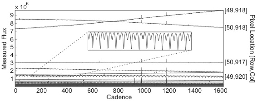
Figure 1: Flux-time series for KID 5041847. The time series for the pixel in which the target falls upon, pixel [50,918], has no observable eclipse signature; however, the time series for pixel [49,920], enlarged in the pop-out, reveals a clear eclipse signature. The target’s pixel coordinates originate from a corner of the appropriate CCD module.

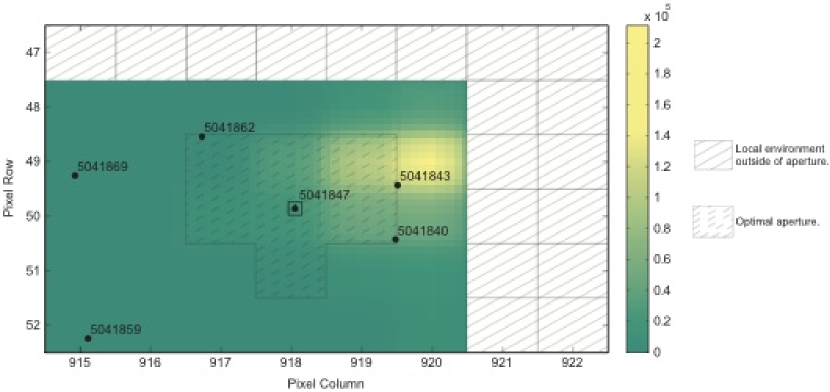
Figure 2: An expanded difference image for target KID 5041847 showing a greater view of the local environment including an overlay of the target’s optimal aperture. This image clearly shows that the pixel with the greatest in-eclipse versus out-of-eclipse difference in flux is not centered on KID 5041847. The true eclipsing binary star is KID 5041843.

After thorough inspection, 58 of the objects included in the first catalog (Paper I) were found to be blended systems where the target star is not itself an EB. The corrected KIDs for these systems are listed in Table 2. These objects have been re-targeted, that is re-centered in optimal apertures, for observation starting in Q8 and have been removed from the catalog pending further observations. Of the former KOIs examined as potential EBs for inclusion into the catalog (§2.1), 172 were found to be blended light curves where the EB component was not the target star. The eclipsing binaries in the blends have been similarly identified and will be added to the target list for observation starting with Q10.

Two overlapping EB systems were discovered during this analysis; both were uncovered as a second EB signature within a target EB s light curve. KID 3437778 and KID 5983351 are the new EBs and their eclipses can be seen superposed in the flux-time series of KID 3437800 and KID 5983348, respectively.

Table 2: Corrected Kepler IDs of Blended EBs

Original KID	Corrected KID	Original KID	Corrected KID	Original KID	Corrected KID
7432476	7432479	5649837	5649836	5392871	5392897
6470521	6470516	10491544	10491554	9075708	9075704
3338674	3338660	7590723	7590728	5041847	5041843
3735634	3735629	7707736	7707742	4073730	4073707
9535881	9535880	9935242	9935245	11825056	11825057
3549993	3549994	11247377	11247386	4579313	4579321
9851126	9851142	8780959	8780968	5816811	5816806
10095484	10095469	8263752	8263746	10743597	10743600
5467126	5467113	8589731	8589754	9456932	9456933
6182846	6182849	8620565	8620561	6233890	6233903
9834257	9773869	7691547	7691553	5730389	5730394
7376490	7376500	6233483	6233466	9366989	9366988
5956787	5956776	9468382	9468384	5020044	5020034
4474645	4474637	6286155	6286161	8647295	8647309
8097897	8097902	6314185	6314173	6312534	6312521
2451721	2451727	5560830	5560831	10747439	10747445
9664387	9664382	6677267	6677264	3335813	3335816
7516354	7516345	5390342	5390351	3446451	3547315
6058896	6058875	5565497	5565486
5022916	5022917	7910148	7910146

2.4 Updating the Ephemerides

With the inclusion of Q2 data, the duration of the light curves increases by a factor of 3.7, so an update of the ephemerides was appropriate. We improved the ephemerides in two steps: First, using a software tool, kalahari, that overlays a cursor cross-hair on the light curve, we selected and centered by eye the first and last occurring clean eclipses in the Q0 through Q2 light curves. This was greatly facilitated by using the previous ephemerides published in Paper I to predict the first and last eclipse; in the vast majority of cases the ephemeris was accurate enough to clearly identify both eclipses and an unambiguous cycle count. These two eclipses were then used to compute a more precise period. An assortment of median, linear, and cubic polynomial detrending options were used to allow combining the different quarters (and discontinuous sections of Q2) together. Phase-folded figures were automatically generated for every system and checked for correctness of the ephemeris—even slight errors in the ephemeris were readily apparent in the phase folded light curves. We estimate the uncertainties in this kalahari manual eclipse selection method to be roughly 50–700 s in the initial epoch of eclipse center, T0, and 0.2–90 s in the period, P, with the shorter period systems giving the higher precision. This “hands on” approach allowed us to visually inspect every light curve and use judgment in the selection of T0, a task that is typically problematic for automated methods. We chose the barycentric Julian day (BJD) of the first good eclipse to define the epoch of eclipse center. This is mainly for convenience. The epoch will not change as more data are added, it places cycle number zero at the start of the light curve, and it makes checking the epoch by users of the catalog relatively easy. In addition, the times are now in BJD, obtained directly from the MAST FITS files, and are not approximated as in Paper I.

Kepler experienced one Safe Mode event and four spacecraft attitude tweaks in Q2 (Christiansen & Machalek, 2011, Table 5), each creating discontinuities in the light curves of various amplitude. In many cases these discontinuities are obvious. However, we caution that in noisy, shallow-eclipse cases, the discontinuity near BJD 2455079.18 is sometimes flagged as an eclipse event triggering a false detection of a periodicity. Similarly, portions of the light curve contain a low amplitude modulation that can sometimes mimic a periodicity. Periods very near $3\fd 00$ and $0\fd 133$ should be treated skeptically, as these may be instrumental in origin (reaction wheel momentum desaturation cycle and focus change due to reaction wheel housing heaters). See the Kepler Data Characteristics Handbook (Christiansen et al., 2011) for these and other important data issues.

The second step of ephemerides determination refines the above estimates by using them as inputs to the ebai engine. Part of the EBAI project (Eclipsing Binaries via Artificial Intelligence), the ebai engine is a back-propagating neural network trained on synthetic eclipsing binary data that is able to quickly determine principal parameters for large numbers of observed light curves (Prša et al., 2008). Its performance on EBs in the first Kepler data release is described in Paper I. We adopted the ebai estimates of T0 as the final values for the ephemerides.

2.5 Catalog Description

The updated catalog contains 2165 eclipsing binaries. Each EB is identified by its Kepler ID in column 1. Its ephemeris, in days, is given in Columns 2 & 3 ($\mathrm{BJD}_{0}$, and $P_{0}$) and subsequent columns contain: morphological classification (Column 4) as one of D (detached), SD (semi-detached), OC (overcontact) , ELV (ellipsoidal variable) or UNC (unclassified); the source of the target (Column 5) which tracks the origin of the added target: CAT if it appeared in the first catalog release, Q1HB if it was held back at the time of the initial release but is now public, KOI if it is a rejected Kepler Object of Interest due to the detected EB signature, and NEW if it was a newly discovered EB; the systems Kepler magnitude (Column 6); and input catalog parameters, $T_{\mathrm{eff}}$ in K (Column 7), $\log\mathrm{g}$ in cgs units (Column 8), $E(\bv)$ (Column 9), and the estimated contamination (Column 10); the principal parameters: $T_{1}/T_{2}$ (Column 11), the scaled sum of the radii $\rho_{1}+\rho_{2}\equiv(R_{1}+R_{2})/a$ (Column 12), the fillout factor $F$ (Column 13), the radial and tangential components of eccentricity $e\sin\omega$ and $e\cos\omega$ (Columns 14 & 15), the mass ratio $q$ (Column 16), and the sine of the inclination $\sin i$ (Column 17).

Table 3: Catalog of EBs in Kepler Q0–2 Data

KID	$\mathrm{BJD}_{0}$	$P_{0}$ [days]	Type	Source	$K\mathrm{mag}$	$T_{\mathrm{eff}}$[K]	$\log\mathrm{g}$ [cgs]	$E(\bv)$	contam
		$T_{2}/T_{1}$	$\rho_{1}+\rho_{2}$	Fillout	$e\sin\omega$	$e\cos\omega$	$q$	$\sin i$
01026032.00	54966.773843	8.460438	D	CAT	14.813	5715	4.819	0.107	0.266
		0.85956	0.12451	$\cdots$	0.05515	0.01308	$\cdots$	0.99687
01026957.00	54956.011753	21.762784	D	KOI	12.559	4845	4.577	0.036	0.034
		0.49053	0.18848	$\cdots$	-0.06237	-0.07830	$\cdots$	0.98538
01433962.00	54965.325203	1.592691	D	KOI	15.470	4349	4.634	0.067	0.609
		0.78423	0.11622	$\cdots$	-0.12883	0.07820	$\cdots$	0.99716
01571511.00	54954.506187	14.021624	D	KOI	13.424	5804	4.406	0.101	0.011
		0.82928	0.13522	$\cdots$	-0.10259	-0.02367	$\cdots$	0.99416
01725193.00	55005.663605	5.926658	D	NEW	14.502	5802	4.384	0.146	0.772
		0.82976	0.23817	$\cdots$	-0.01015	0.05277	$\cdots$	0.97561
01996679.00	54979.068748	20.000276	D	KOI	13.884	5914	4.334	0.119	0.018
		0.69915	0.13037	$\cdots$	-0.14132	0.16568	$\cdots$	0.99437
02010607.00	54974.583000	18.627229	D	CAT	11.347	6122	4.344	0.056	0.065
		0.76403	0.12954	$\cdots$	-0.11481	0.03654	$\cdots$	0.99506
02162635.00	55009.129448	$\cdots$	D	KOI	13.862	4787	3.567	0.160	0.061
		$\cdots$	$\cdots$	$\cdots$	$\cdots$	$\cdots$	$\cdots$	$\cdots$
02162994.00	54965.631839	4.101588	D	CAT	14.162	5410	4.532	0.099	0.189
		0.86621	0.18990	$\cdots$	-0.06236	0.00060	$\cdots$	0.99798
02305372.00	54965.963928	1.404636	D	CAT	13.821	5664	3.974	0.158	0.267
		0.51753	0.59250	$\cdots$	-0.00898	-0.00365	$\cdots$	1.00256
02305543.00	55003.400185	1.362339	D	NEW	12.545	5623	4.486	0.064	0.001
		0.87172	0.31464	$\cdots$	-0.03268	0.01347	$\cdots$	0.97667
02306740.00	54987.038258	10.307175	D	CAT	13.545	5647	4.228	0.117	0.241
		0.86225	0.13727	$\cdots$	-0.11561	0.02030	$\cdots$	0.99919
02308957.00	54965.169838	2.219736	D	CAT	14.520	5697	4.343	0.148	0.649
		0.95548	0.46031	$\cdots$	-0.00715	0.01505	$\cdots$	0.98274

Note. — Table 3 is published in its entirety in the electronic edition of the Astronomical Journal. A portion is shown here for guidance regarding its form and content.

3 Interesting Objects in the Catalog

3.1 Tertiary Eclipses

The search for circumbinary planets in the Kepler data includes looking for transits with multiple components (e.g. Deeg et al., 1998; Doyle et al., 2000). Transit patterns with multiple components are caused by a slowly moving planet crossing in front of the eclipsing binary; it is alternately silhouetted by the motion of the background binary stars as they orbit about each other. Circumbinary transits can thus produce predictable but non-periodic features of various shapes and depths. We have been looking for such features in the Catalog and, in the process, have identified several tertiary eclipses where the depth of each event is, in most cases, too deep to be the transit of a planet but is, instead, an eclipse by a third (sub-)stellar body. In Fig. 3 we show 4 such systems illustrating the variety of ”transit signatures” that can be produced and discuss each system in turn in what follows.

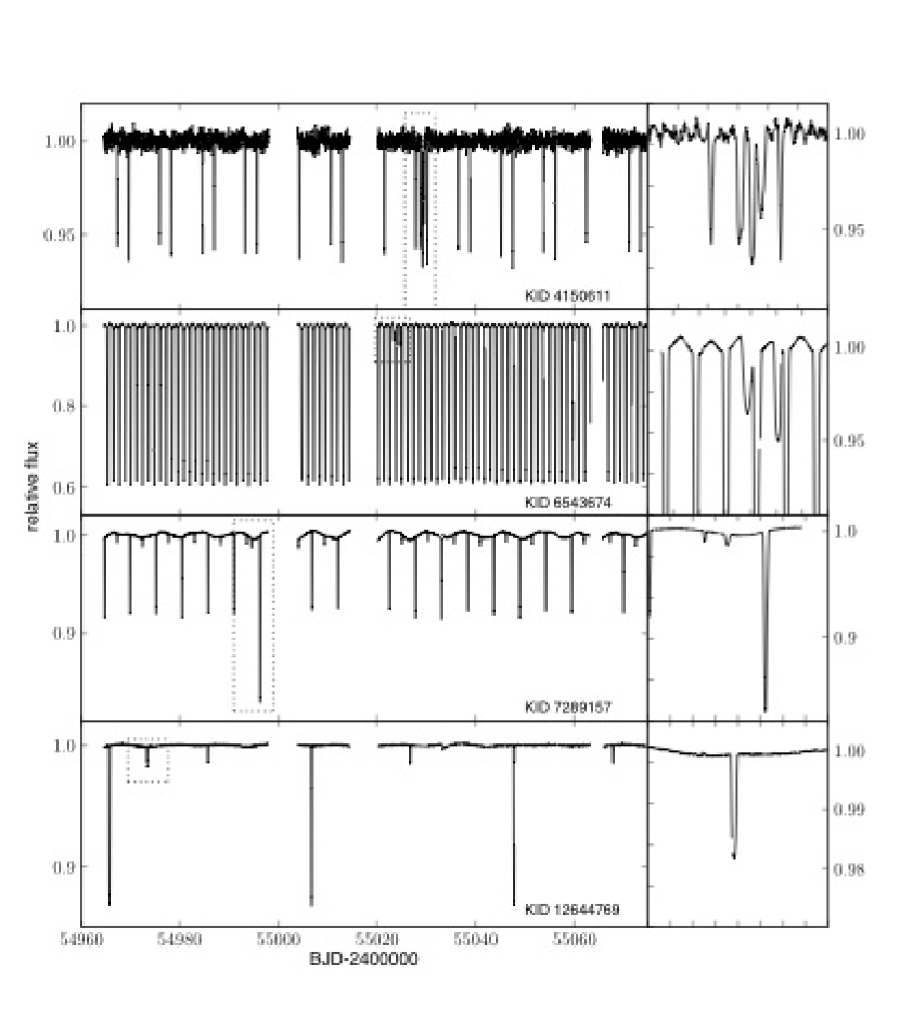
Figure 3: Four EBs with significant tertiary eclipse events. The systems are (top to bottom): KID 4150611 ($P=8\fd 65308$), 6543674 ($P=2\fd 39105$), 7289157 ($P=5\fd 26627$), and 12644769 ($P=41\fd 0781$). The Q1+Q2 light curve for each system is shown on the left with the tertiary event marked with a dashed box. On the right is an expanded region around the anomalous event.

KID 4150611 ($P=8\fd 65308$) shows a series of grazing eclipses. The system is bright, Kep${}_{m}=7\fm 889$, yet very “noisy” with a Kepler Input Catalog (KIC) temperature, $T_{\mathrm{eff}}=6623$ K suggesting a mid-F type star undergoing $\delta$ Sct oscillations. A triplet event can be seen between the primary and secondary eclipses near the middle of the light curve which is somewhat puzzling. The short, $0\fd 7$ duration of the triple event occurs while the EB is out-of-eclipse so it cannot be a single third-body transiting the EB as that would result in only two dips. A more plausible model has a short-period binary system transiting one of the EB components similar to the KID 5897826 system discussed below. That is a quadruple system consisting of two binary systems where one of the systems is eclipsing. Another possibility we are considering is that the light curve is the composite of an hierarchical triple, the F-star and the short-period binary, plus an additional eclipsing binary either physically associated with the triple or simply a blend.

KID 6543674 ($P=2\fd 390105$) is a shorter period EB with deep eclipses from two nearly equal components seen close to edge-on. Their separation is small enough that mutual tidal forces are distorting the stars yielding the distinct out-of-eclipse ellipsoidal (aspect) variations which are readily seen in the expanded box on the right. There are two tertiary eclipses separated by $1\fd 2$ which is consistent with the model of a single third-body passing in front of the EB and being alternately silhouetted by the EB components as they orbit one another. This system also has eclipse timing variations (§3.2, Fig. 4) that may arise from the light time effect as the third-body orbits that binary.

KID 7289157 ($P=5\fd 26627$) has two tertiary events less than two days apart with the second event coinciding with a primary eclipse. The depth of a transit in a binary system is shallower than in the equivalent single star case as flux from the non-transited binary component diluting the transit signature. When a transit occurs during an eclipse, the dilution is significantly reduced yielding a deeper transit dip as has happened here. Like HD 6543679, this system also has eclipse timing variations (Fig. 5) but with a significantly larger amplitude and large a discrepancy between primary and secondary times. Dynamical interactions will need to be considered to understand this system.

KID 12644769 ($P=41\fd 0781$) has a single extra event in the light curve during Q1 with a depth of slightly less that $\lesssim 2\%$. With only a single event, one cannot rule out a blend with a long period background EB and we do note that this feature is slightly deeper than the secondary eclipses. The event is potentially interesting considering the photometrically derived stellar parameters for this system in the KIC suggests that the components are late-K or M-dwarfs. ($T_{\mathrm{eff}}=4051$ K, $\log g=4.48$, radius$=0.74$). If so, they imply that the radius of the transiting body is $\lesssim 2R_{\mathrm{Jup}}$ and that there may be a sub-stellar object orbiting this system.

These and other tertiary events are being studied and will be further described in an upcoming paper (Doyle et al., 2011).

Table 4: Significant Tertiary Eclipse Events during Q1 and Q2

Kepler ID	Event	Mid-time	Mid-event depth
	(Fig.3)	[2400000-BJD]	[mag]
04150611	1	55028.9	0.0630
	2	55029.3	0.0745
	3	55029.6	0.0502
06543674	1	55023.5	0.0500
	2	55024.7	0.0644
07289157	1	54994.6	0.0105
12644769	1	54973.4	0.0204

Finally, another eclipsing binary with tertiary eclipses, KID 5897826 (KOI-126), was described in detail by Carter et al. (2011). It consists of two M-dwarfs in a 1$\fd$77 mutual orbit, which itself orbits around a slightly evolved $1.35\,M_{\odot}$ primary star with a 33$\fd$9 orbit. Each time the M-dwarfs pass in front of the primary, they give rise to two $\sim 1.5$% deep, transit-shaped events, which are often superimposed due to the relative phasing of the small and large orbits, and distorted due to the acceleration of the M-dwarfs by each other during the transit across the primary. Eclipses between the M-dwarfs are also seen at the beginning of the dataset but their depths are reduced to zero as the primary causes their orbits to precess into a non-eclipsing inclination. Besides being a dramatic demonstration of dynamical interactions in a triple-star system, dynamical fits produced a measurement of masses ($0.2413\pm 0.0030\,M_{\odot}$ and $0.2127\pm 0.0026\,M_{\odot}$) and radii ($0.2543\pm 0.0014\,R_{\odot}$ and $0.2318\pm 0.0013\,R_{\odot}$) for two M-dwarfs, a valuable test of theoretical stellar structure models.

3.2 Eclipse Timing Variations

Table 5: EBs with eclipse timing variations

KID	$P_{\rm prim}$	$P_{\rm sec}$	O-C range, primary	O-C range, secondary
	(d)	(d)	(min)	(min)
05771589	$10.7379\phantom{0}\phantom{0}\phantom{0}\phantom{0}\pm 0.0023$	$10.7374\phantom{0}\phantom{0}\phantom{0}\phantom{0}\pm 0.0014$	140	89
06543674	$\phantom{0}2.39104706\pm 0.000003$	$\phantom{0}2.39104110\pm 0.000006$	2.4	1.2
06545018	$\phantom{0}3.99144\phantom{0}\phantom{0}\phantom{0}\pm 0.00008$	$\phantom{0}3.99143\phantom{0}\phantom{0}\phantom{0}\pm 0.00009$	17	18
07289157	$\phantom{0}5.26585\phantom{0}\phantom{0}\phantom{0}\pm 0.00001$	$\phantom{0}5.26625\phantom{0}\phantom{0}\phantom{0}\pm 0.00010$	1.9	15
07668648	$27.7828\phantom{0}\phantom{0}\phantom{0}\phantom{0}\pm 0.0050$	$27.7976\phantom{0}\phantom{0}\phantom{0}\phantom{0}\pm 0.0005$	35	2.7
07955301	$15.3225\phantom{0}\phantom{0}\phantom{0}\phantom{0}\pm 0.0047$	$15.3196\phantom{0}\phantom{0}\phantom{0}\phantom{0}\pm 0.0045$	137	169
09714358	$\phantom{0}6.4739\phantom{0}\phantom{0}\phantom{0}\phantom{0}\pm 0.0004$	$\phantom{0}6.4738\phantom{0}\phantom{0}\phantom{0}\phantom{0}\pm 0.0003$	42	41
10319590	$21.3273\phantom{0}\phantom{0}\phantom{0}\phantom{0}\pm 0.0013$	$21.3227\phantom{0}\phantom{0}\phantom{0}\phantom{0}\pm 0.0009$	20	8

In an EB, one normally expects the primary eclipses to be uniformly spaced in time. However, mass transfer from one star to the other or the presence of a third star in the system can give rise to changes in the orbital period, which in turn will change the time interval between consecutive eclipse events. The eclipse times will no longer be described by a simple linear ephemeris, and the deviations (usually shown in the “O-C” diagram) will contain important clues as to the origin of the period change. We have begun to systematically measure the times of primary and secondary eclipse for the Kepler sample of EBs classified as detached (D) and semidetached (SD). This is a difficult task, owing to a host of intrinsic variabilities and systematic problems. These include large spot modulations that may or may not be in phase with the eclipses, pulsations and/or noise in the out-of-eclipse regions, thermal events and cosmic ray hits that make the normalization of the light curves hard to automate, and eclipses falling partially or completely in data gaps. This work will be fully described in an upcoming paper (Orosz et al., 2011). We present here some interesting cases of EBs with O-C variations evident in the Q0–Q2 data.

Briefly, these basic steps are followed to measure the times of eclipse. (i) The light curve is detrended quarter by quarter and combined. (ii) The ephemeris is determined, and (iii) the light curve is phased based on the ephemeris values. (iv) A simple function of the form $y=x^{n}$, where $n$ is not necessarily an integer, is fit to half of the eclipse profile and then reflected to the other half. Finally, (v) the light curve is unfolded, and the mean profile is fit to individual events after an additional local de-trending is applied to obtain the eclipse time. In some cases, an automated code was able to set the limits of the local fitting on its own, and in other cases, it was necessary to specify the fitting limits manually. A linear ephemeris is fitted to the times, and the O-C diagram is generated. The typical uncertainties in the individual times range from about 30 seconds in the best cases to around two minutes for cases with noisy out-of-eclipse regions (where the “noise” can be due to spot modulations or pulsations in addition to shot noise).

At the time of this writing, about half of the sample has been completed. The O-C diagrams were inspected visually, and eight cases where the O-C diagram has a significant signal through Q2 were identified, see Figs. 4 and 5. KID 5771589 and KID 7955301 have changes in their O-C diagrams of more than 100 minutes. Most of the others have changes of 20 to 40 minutes. It seems unlikely that such large changes in the O-C diagram over such short times ($\approx 125$ days) can be caused only by light travel time effects. We also note that the timescale for apsidal motion is much longer than the variations seen here. Hence, each of these EBs is most likely interacting with a third body.

The list of eight systems includes two of the four EBs with tertiary eclipses, namely KID 6543674 and KID 7289157. KID 6543674 has a modest sized, but coherent signal in both the primary and secondary curves. On the other hand, the secondary eclipses of KID 7289157 show roughly a 10 minute O-C variation, whereas the primary eclipses are consistent with a constant period. In a similar fashion, both KID 10319590 and KID 7668648 have O-C variations of the primary eclipses that are a bit different than the O-C variations of the secondary eclipses, although the number of events in each is not that large. If confirmed with more data, these period differences between the primary eclipses and secondary eclipses would almost certainly be a sign of a dynamical interaction with another body.

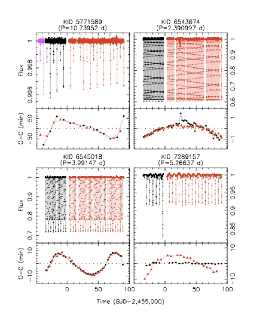
Figure 4: EBs with a significant signal in the O-C diagram. The normalized light curves are shown in the upper parts of each panel where the different colors correspond to data from different quarters, and the O-C diagram with curves for the primary (filled circles) and secondary (filled triangles) eclipses are shown in the lower parts of each panel. KID 6543674 and KID 7289157 have tertiary eclipses.

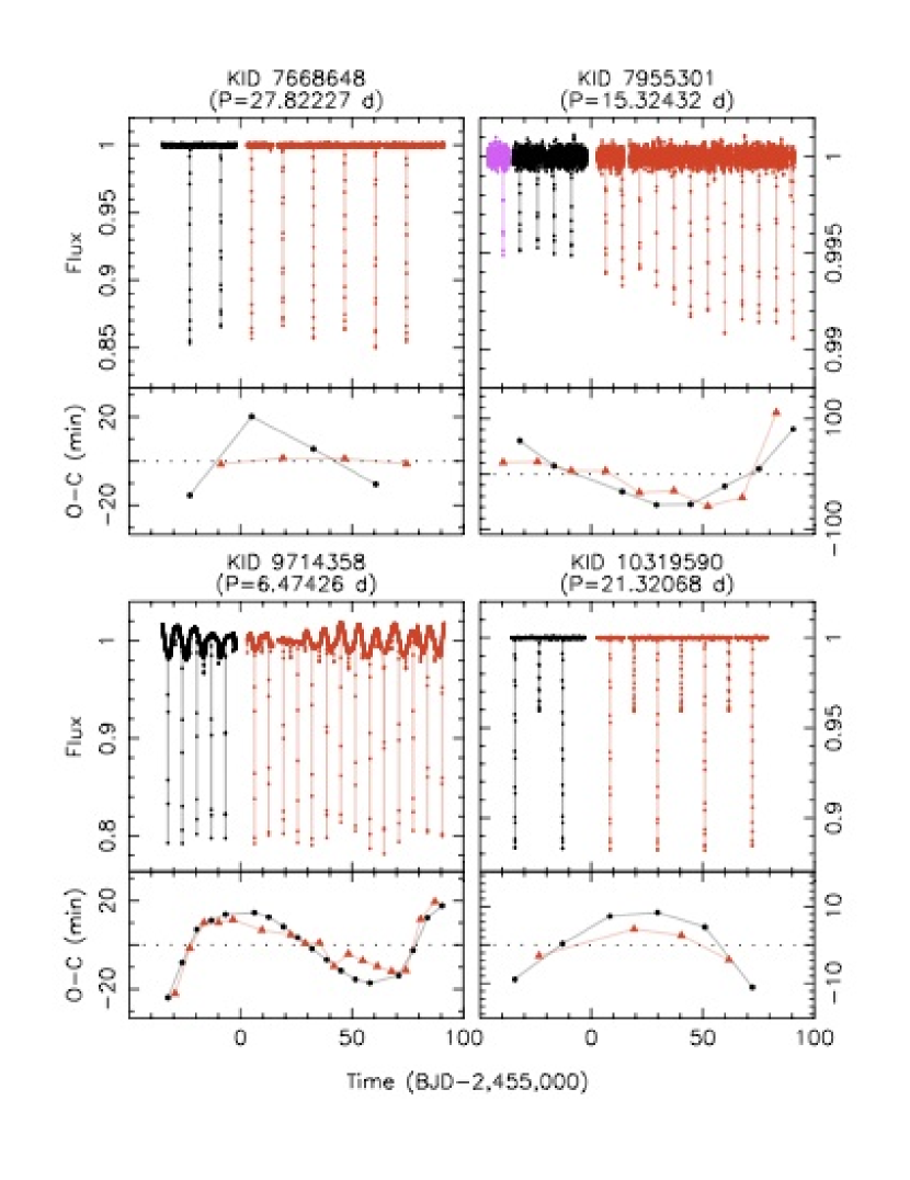
Figure 5: EBs with significant signals in the O-C diagram. The normalized light curves are shown in the upper parts of each panel where the different colors correspond to data from different quarters, and the O-C diagram with curves for the primary (filled circles) and secondary (filled triangles) eclipses are shown in the lower parts of each panel.

Finally, KID 7955301 seems to have a systematic change in the eclipse depth. One should be cautious when interpreting changes in the eclipse depth from quarter to quarter (§4.1). If the eclipse depths really are getting deeper in KID 7944301, then that fact should become increasingly evident as more data become available.

4 Updated Parameters

4.1 Potential Quarter-to-Quarter Systematics

In order to keep its solar panels aligned with the Sun, the Kepler spacecraft must roll by 90° four times a year. The spacecraft orientation at a given angle defines “quarters”, and the spacecraft had a different orientation during Q2 than it had during Q0/1 (there was no roll between Q0 and Q1). As a result the stars are on different CCDs during Q2 compared to Q0/1. In addition, the optimal photometric apertures may be quite different from quarter to quarter particularly for faint stars, and if an EB is in a crowded field, the amount of blending with other sources may likewise change from quarter to quarter. We have found several cases with abrupt changes in the eclipse depth between Q1 and Q2, and these are almost certainly caused by differences in the contamination levels. Figure 6 shows four such cases. These are all clearly EBs, but the eclipse depths of a few percent or less indicates a high level of contamination. Three of these have been shown to be blends where the targeted object was not the EB (see §2.3 above) and have been retargeted beginning with Q8. Users of Kepler data are urged to use caution when combining data crossing quarter boundaries.

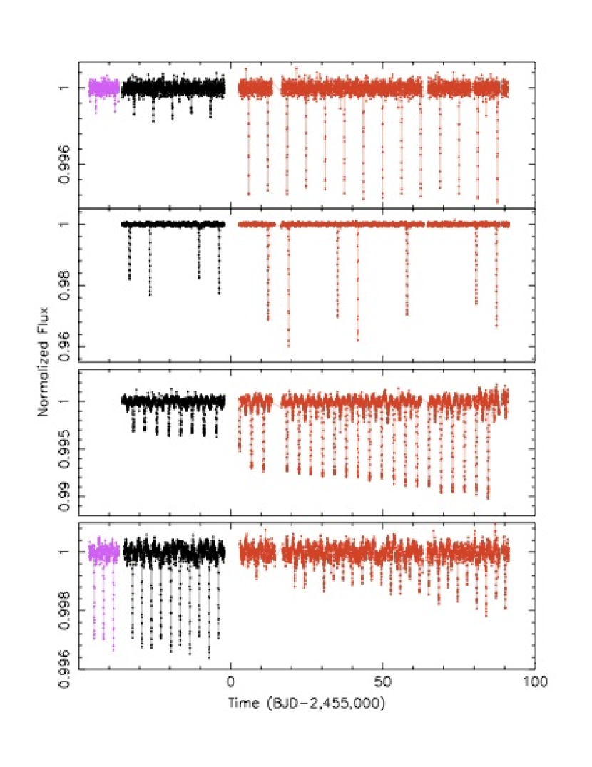
Figure 6: Examples of EBs suffering from systematic errors owing to changes in the contamination level from quarter to quarter. To highlight the point, the data from different quarters are shown by different colors. The EBs are, from top to bottom, KID 8255058 ($P=6\fd 28383$), KID 10491544 ($P=22\fd 7729$), KID 4474645 ($P=3\fd 98084$), and KID 4073730 ($P=6\fd 27129$).

4.2 Data Detrending

One of the main issues that prevents reliable catalog-wide EB light curve fitting is variability in the baseline flux level. This may be the result of either systematic effects (focus drifts, safe modes, etc. – see Christiansen & Machalek 2011), intrinsic stellar variability (chromospheric activity, pulsations), or extrinsic contamination by third light (a variable source that contributes light in the aperture of the object of interest). The main Kepler pipeline delivers two types of photometric data: calibrated and corrected. Calibrated data are obtained by performing pixel-level calibration that corrects for the bias, dark current, gain, non-linearity, smear and flat-field, and applies aperture photometry to reduced data. Corrected data are the result of Pre-search Data Conditioning (PDC) that corrects degraded cadences due to data anomalies and removes variability to make the targets suitable for planet transit detection (Jenkins et al., 2010b). Since the PDC detrending is optimized for planet transits, its effects on eclipsing binary data are found to be adverse in a significant fraction of all cases (cf. the discussion in Paper I, §2). That is why we use only calibrated data in our analyses. As a consequence, the detrending of data needs to be done as part of our processing pipeline.

The basis of the implemented data detrending algorithm is a least squares Legendre polynomial fit of order $k$ to the data. The initial fit takes all data points into account. Since we want to fit the baseline, we sigma-clip data points to the asymmetric interval $(-1\sigma,3\sigma)$: any points that are $1\sigma$ below the fit and $3\sigma$ above the fit are discarded. We re-fit the polynomial to the remaining data points and perform the next clipping iteration. The process continues until no data points are clipped. The fitted polynomial approximates the variable baseline and we divide the observed data by the polynomial value at each cadence. This results in a normalized, detrended light curve that is subsequently phased with the respective ephemeris and passed to the modeling engine ebai.

Multi-quarter data present a challenge for this approach because of the discontinuities in the light curves caused by anomalies and random cosmic ray events. To account for predictable discontinuities (documented in Christiansen & Machalek 2011), we split the whole data sequence into parts with boundaries at each discontinuity and detrend each part separately. The detrending polynomial order $k_{i}$ for part $i$ is computed automatically from the number of data points so that $k_{i}=(N_{i}/N)k$, where $N$ is the total number of data points and $k$ is the suitable polynomial order for the whole data span. Our attempts to determine the detrending order $k$ automatically had limited success, so for the most part a manual inspection was used. Fig. 7 depicts a detrending example of order $k=150$ for KID 12506351 – a case of a detached binary with a strongly variable baseline due to significant chromospheric activity.

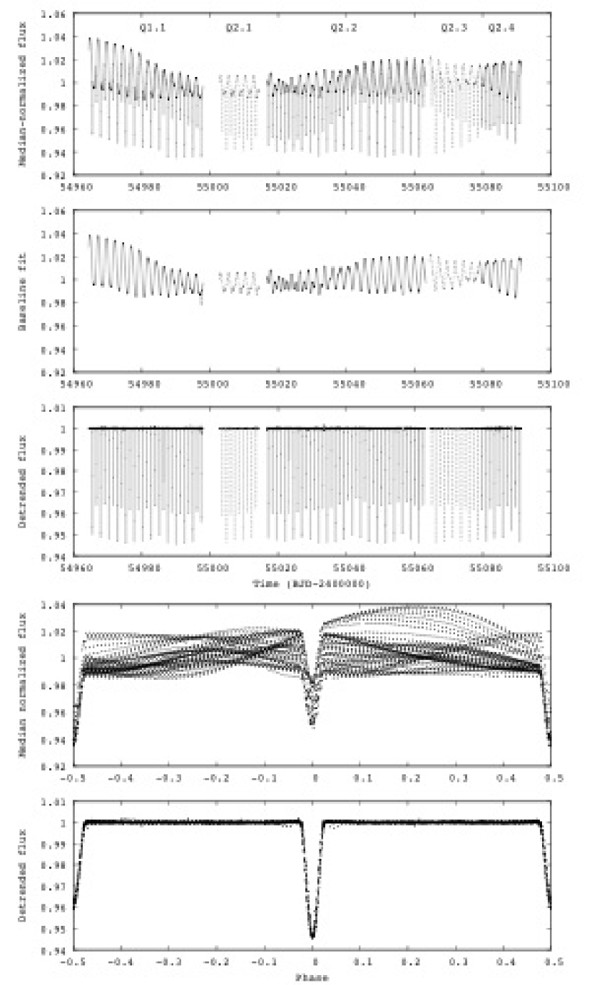
Figure 7: An example of the detrending algorithm performance on a detached binary KID 12506351 with a strongly variable baseline. The set is split into 5 parts at the predictable discontinuities: Q1 and 4 sub-parts of Q2: Q2.1, Q2.2, Q2.3 and Q2.4. The successive panels show (top-to-bottom): the median-normalized light curve, the fitted baseline solution, the detrended light curve, the original phase curve, and the detrended phase curve.

To facilitate modeling of phased light curves (or even make it possible in some cases), aggressive detrending needs to be applied to the data. This is most notable for chromospherically active stars where spot modulation causes a significant baseline variability with an amplitude of the same order as the eclipse depths. In such cases the detrending is likely to adversely remove variability due to ellipsoidal variations as well. In order to prevent the negative effects of detrending on eclipses, we limit the largest fitting polynomial period to the orbital period and warn that, despite our best effort, processing artifacts are likely injected into the most variable data-sets and detailed manual detrending remains necessary.

It is very difficult to automatically detrend random discontinuities in EB data mostly because eclipses in detached binaries are discrete discontinuities. At this time we ignore such discontinuities since their impact on the light curve solution is seldom critical. However, we are in the process of implementing a feedback loop from the part of the pipeline that phases the data: the eclipses are detected and removed, and the data whitened in this way are subject to a discontinuity search. If a discontinuity is found, a new breakpoint is added and the set is divided into new subsets. The first results seem promising, but further testing and validation is required before this detrending approach is implemented into the pipeline.

5 Catalog Analysis

In this section we provide an updated look at several distributions of the eclipsing binaries within the Kepler field-of-view. In Paper I we showed the distribution of EBs as a function of their orbital period stacked by their morphological type. The short Kepler Q1 baseline of 34 days limited the analysis to periods less than 25 days. Here we have re-plotted the distributions in $\log$-Period and examine the distributions with temperature after dividing the EBs into two subsets, the detached and semi-detached systems in Figs. 8 and 9, and the over-contact and ellipsoidal systems in Figs. 10 and 11.

There is a distinct fall-off in the number of detached systems at both shorter, $P\lesssim 0\fd 8,$ and longer, $P\gtrsim 45^{d}$, periods. The short fall-off is due to the relatively small number of low-mass systems in the magnitude limited Kepler target catalog. Such EBs have as components late-K and M dwarf stars that would be expected to populate this part of the distribution. In Fig. 9, we show the distribution of detached EBs from the catalog with their effective temperature as listed in the Kepler Input Catalog. This shows the sharp decline in the number of systems with decreasing temperature, again indicative of the same selection effect. We caution that the effective temperatures in the KIC, which apply to single stars, have large uncertainties ($\pm 300$ K or more). Also, no correction has been applied for binarity which may lead to an underestimate of the temperature of the hotter (usually primary) component. The fall-off at periods longer than $\sim 45$ days indicates where incompleteness begins to become significant. Another feature in Fig. 8 is the possible excess of detached systems with periods near 5 days although it is not clear how significant it is.

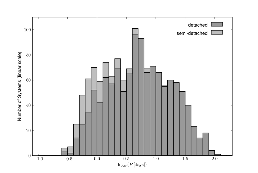
Figure 8: Period distribution of the detached (darker grey) and semi-detached (lighter grey) eclipsing binary systems in the Kepler Q1+Q2 data set. The baseline is 125 days ($\log P=2.1$).

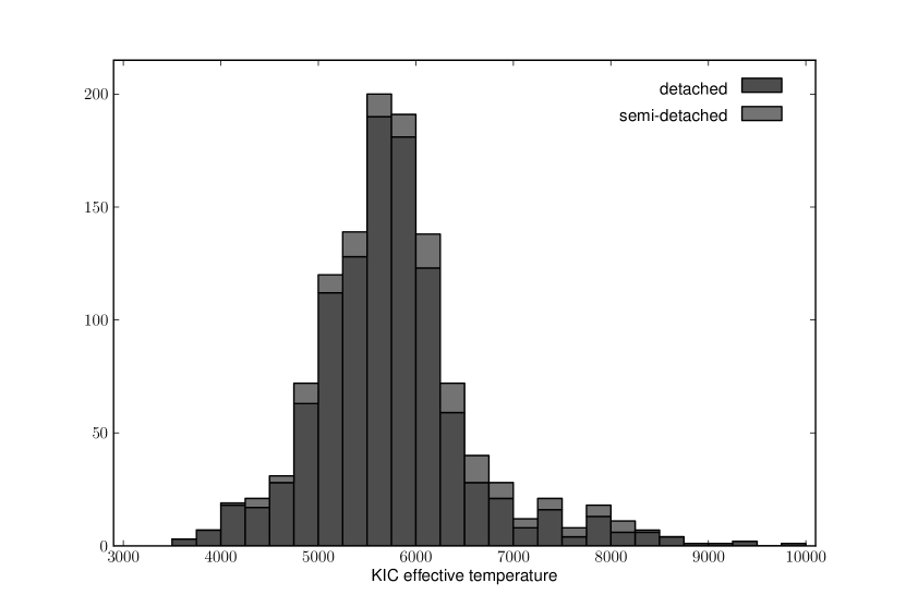
Figure 9: Distribution of detached EBs with Kepler Input Catalog effective temperature.

The log-period distribution of overcontact systems (Fig. 10) has a prominent peak near $-0.5$ ($\sim$0.3 days) and a smaller, perhaps broader component centered about $-0.2$ ($\sim$0.65 days). This is suggestive of two separate populations. In Fig. 11 we show the KIC temperature distribution for the contact systems. Interestingly, this distribution has a slight skew towards higher temperatures whereas the temperature distribution of the detached systems has a slight skew to lower temperatures.

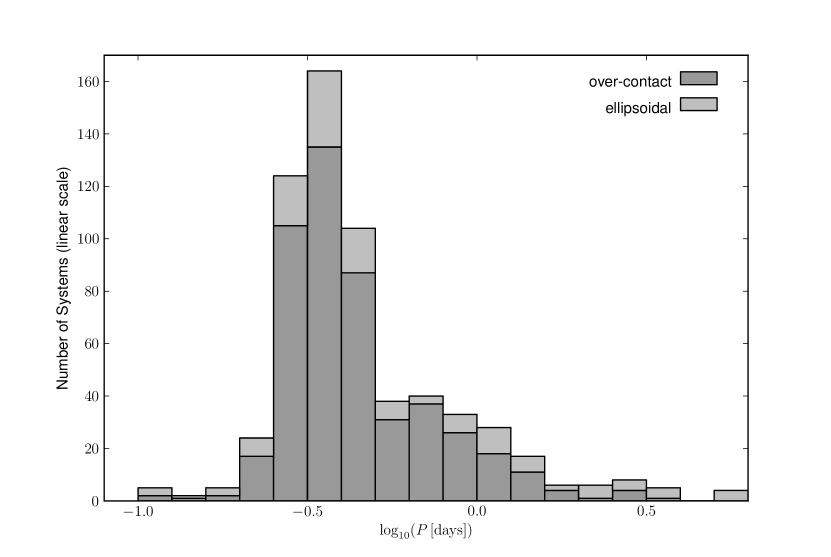
Figure 10: Period distribution of the over-contact and ellipsoidal systems in the second Kepler  data release.

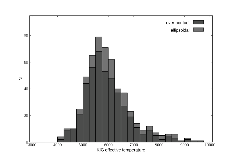
Figure 11: Distribution of over-contact and ellipsoidal systems with KIC effective temperature.

Figure 12 is an update of Fig. 12 in Paper I. It shows a variation in the fraction of targets that are eclipsing binaries with galactic latitude. In general, there is an increase in the EB fraction due to the increase in the number of systems in the updated catalog.

There is a nearly uniform distribution in the eclipsing binary fraction with latitude for the short-period, interacting overcontact and semi-detached systems, and the ellipsoidal variables. This indicates a large scale-height perpendicular to the galactic plane for these EBs suggestive of an older population. In contrast, the detached systems become an increasingly larger fraction of the targets at lower galactic latitudes. While some of this may be due to increased crowding resulting in a larger number of blends, it also points to a greater concentration of detached systems towards the galactic plane, implying that these EBs are, on average, younger.

Finally, at the higher galactic latitudes, the total eclipsing binary fraction is observed to flatten out at $\sim$1.1–1.2%, essentially the same fraction found in Paper I.

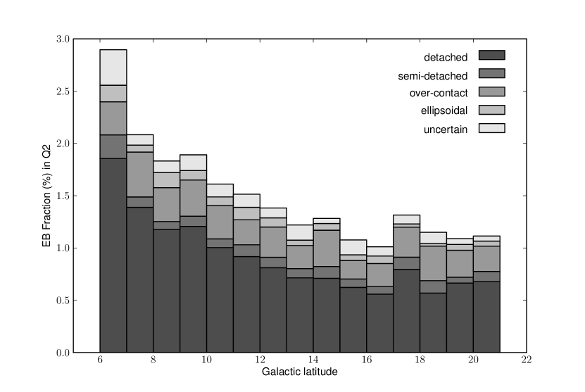
Figure 12: The percentage fraction of Q2 targets classified as EBs in each $1^{\circ}$ strip of galactic latitude within the Kepler FOV. Different morphological types are indicated in grey-scale. The first and last bin are affected by the small number of objects in the strips containing the FOV edges.

6 Summary

The revised catalog of eclipsing binaries contains 2165 entries: 1261 detached, 152 semi-detached, 469 overcontact, 137 ellipsoidal variables and 147 uncertain or unclassified systems. All new entries have been subjected to the same level of scrutiny as the initial catalog targets: the periods were determined by using ephem and sahara tools (Paper I) and the folded light curves examined for any clear non-EB signatures. All ambiguous cases were flagged as uncertain (UNC) and require further validation.

This revision of the catalog contains a new column Source. It tracks the origin of the added target: CAT if it appeared in the first catalog release, Q1HB if it was held back at the time of the initial release but is now public, KOI if it is a rejected Kepler Object of Interest due to the detected EB signature, and NEW if it was a newly discovered EB.

An online version of the catalog is maintained at http://keplerEBs.villanova.edu. This catalog lists Kepler ID, morphology, ephemeris, principle parameters, and figures with both time domain and phased light curves of each system. It is recommended that anyone wishing to use Kepler data for any of these systems consult the updated Data Release Notes for quarters Q0 and Q1 (first data release), and Q2 (second data release) that are available at the MAST website^,.

References

- Basri et al. (2011) Basri, G., et al. 2011, AJ, 141, 20
- Batalha et al. (2010) Batalha, N. M., et al. 2010, ApJ, 713, L109
- Borucki et al. (2010a) Borucki, W. J., et al. 2010a, Science, 327, 977
- Borucki et al. (2010b) Borucki, W. J.; for the Kepler Team, 2010b, arXiv:1006.2799v2 [First Data Release]
- Borucki et al. (2011) Borucki, W., et al. 2011, arXiv:1102.0541 [Second Data Release]
- Bryson et al. (2010) Bryson, S., et al. 2010, ApJ, 713, L97
- Bryson et al. (2011) Bryson, S., et al. 2011 (in preparation)
- Caldwell et al. (2010) Caldwell, D. A., et al. 2010, ApJ, 713, L92
- Carter et al. (2011) Carter, J. A., et al. 2011, Science, 331, 562
- Christiansen & Machalek (2011) Christiansen, J. & Machalek, P. 2011, Kepler Data Release 7 Notes
- Christiansen et al. (2011) Christiansen, J. et al. 2011, Kepler Data Characteristics Handbook, KSCI-19040-001 (available from http://archive.stsci.edu/kepler/documents.html)
- Coughlin et al. (2010) Coughlin, J. L., L pez-Morales, M., Harrison, T. E., Ule, N., Hoffman, D. I. 2010, arXiv:1007.4295v3
- Debosscher et al. (2011) Debosscher, J., et al. 2011 (in preparation)
- Deeg et al. (1998) Deeg, H.-J., et al. 1998, A&A, 338, 479
- Doyle et al. (2000) Doyle, L. R. et al. 2000, ApJ, 535, 338
- Doyle et al. (2011) Doyle, L. R. et al. 2011 (in preparation)
- Gilliland et al. (2010) Gilliland, R. L., et al. 2010, ApJ, 713, L160
- Jenkins (2002) Jenkins, J. M. 2002, ApJ, 575, 493
- Jenkins et al. (2010a) Jenkins, J. M., et al. 2010a, ApJ, 713, L120
- Jenkins et al. (2010b) Jenkins, J. M., et al. 2010b, ApJ, 713, L87
- Jenkins et al. (2010c) Jenkins, J. M., et al. 2010c, SPIE Conf. Ser. 7740E, 10
- Koch et al. (2010) Koch, D. G., et al. 2010, ApJ, 713, L79
- Morrison et al. (2011) Morrison, S., Mighell, K., Howell, S., & Bradstreet, D. 2011, BAAS, 43, Abstract 140.15
- Orosz et al. (2011) Orosz, J., et al. 2011 (in preparation)
- Prša et al. (2008) Prša, A., Guinan, E. F., Devinney, E. J., DeGeorge, M., Bradstreet, D. H., Giammarco, J. M., Alcock, C. R., & Engle, S. G. 2008, ApJ, 687, 542
- Prša et al. (2011) Prša, A., et al. 2011, AJ, 141, 83
- Rowe et al. (2010) Rowe, J. F., et al. 2010, ApJ, 713, L150
- Wilson (1979) Wilson, R. E. 1979, ApJ, 234, 1054