Properties of Dark Matter Haloes and their Correlations: the Lesson from Principal Component Analysis

Abstract

We study the correlations between the structural parameters of dark matter haloes using Principal Component Analysis (PCA). We consider a set of eight parameters, six of which are commonly used to characterize dark matter halo properties: mass, concentration, spin, shape, overdensity, and the angle ($\Phi_{L}$) between the major axis and the angular momentum vector. Two additional parameters ($x_{\rm off}$ and $\rho_{\rm rms}$) are used to describe the degree of ‘relaxedness’ of the halo. We find that we can account for much of the variance of these properties with halo mass and concentration, on the one hand, and halo relaxedness on the other. Nonetheless, three principle components are usually required to account for most of the variance. We argue that halo mass is not as dominant as expected, which is a challenge for halo occupation models and semi-analytic models that assume that mass determines other halo (and galaxy) properties. In addition, we find that the angle $\Phi_{L}$ is not significantly correlated with other halo parameters, which may present a difficulty for models in which galaxy disks are oriented in haloes in a particular way. Finally, at fixed mass, we find that a halo’s environment (quantified by the large-scale overdensity) is relatively unimportant.

1 Introduction

In the paradigm of hierarchical structure formation, gravitational evolution causes dark matter particles to cluster around peaks of the initial density field and to collapse into virialized objects (haloes), which provide the potential wells in which galaxies subsequently form (White & Rees 1978). It is therefore expected that the properties of a galaxy are correlated with the properties of its host halo. Small haloes merge to form larger and more massive haloes, which tend to be located in dense environments and are expected to host groups of galaxies.

It is commonly assumed that the mass of a dark matter halo determines how the galaxies it hosts form and evolve; other halo properties are assumed to be less important at fixed mass. This assumption is usually made both by those who use halo models of galaxy clustering (e.g., Zehavi et al. 2005; Skibba et al. 2006; van den Bosch et al. 2007; Moster et al. 2010) and by those who use semi-analytic models of galaxy formation (e.g., Bower et al. 2006; De Lucia & Blaizot 2007; Cattaneo et al. 2007; Somerville et al. 2008). Many of such models have recently been able to provide a description, and perhaps a plausible explanation, of various galaxy statistics, such as the luminosity function, stellar mass function, colour-magnitude distribution, correlation function, and mark correlation functions, lending credence to claims about the importance of halo mass.

Nonetheless, although halo properties, such as their mass, spin, concentration, and shape are correlated with each other, there is considerable scatter in these correlations (e.g., Avila-Reese et al. 2005; Macciò et al. 2007; Macciò et al. 2008; Ragone-Figueroa et al. 2010). In addition, recent studies of numerical simulations have shown that halo formation time is correlated with the environment at fixed mass (e.g., Sheth & Tormen 2004; Gao et al. 2005; Dalal et al. 2008). Some have argued that the halo occupation distribution (used in models of galaxy clustering) is correlated with formation time at fixed mass (Zentner et al. 2005a; Wechsler et al. 2006; Giocoli et al. 2010). It has also been argued that such halo ‘assembly bias’ affects the clustering of galaxies and that the effect varies with luminosity and colour (Croton et al. 2007). Nonetheless, careful studies of the environmental dependence of galaxy luminosity and colour in the real universe have explained this dependence in terms of the environmental dependence of halo mass alone (e.g., Tinker et al. 2008a; Skibba & Sheth 2009). Such models are also encouraged by an analysis of a halo-based galaxy group catalogue, in which, given a halo’s mass, the colours of the galaxies it hosts are not significantly correlated with the large-scale density field (Blanton & Berlind 2007). In addition, the halo model can reproduce the observed non-monotonic relation between clustering strength and density (Abbas & Sheth 2007); note, however, that assembly bias effects are thought to be stronger for lower mass haloes (e.g., Croton et al. 2007; Wang et al. 2007), which host fainter galaxies than the SDSS can reliably probe. The results of these studies suggest that assembly bias affects the formation of observed galaxies only weakly, if at all, although the debate is not yet resolved.

It is also commonly assumed that typical dark matter haloes are relaxed and in virial equilibrium. Nevertheless, Macciò et al. (2007) have shown that many haloes are significantly unrelaxed, sometimes because they are experiencing or have recently experienced a merger or have not yet virialized. In addition, statistical studies of galaxy groups and clusters have shown that the most massive galaxy in these systems is often significantly offset from the centre of the potential well, which may be an indication that some of the systems are unrelaxed (van den Bosch et al. 2005; Skibba et al. 2011).

The relation between halo formation and galaxy formation is far from clear, and these issues are in need of further investigation. For example, to what extent halo mass determines other halo properties, and to what extent relaxed and unrelaxed haloes differ, remains to be seen. The purpose of this paper is to examine the properties of dark matter haloes in numerical simulations, with principal component analysis (PCA). This type of analysis allows us to quantify the correlations between the halo properties, determine which properties are the most important, and to what extent halo mass is the dominant property. It also allows us to characterize the distinctive properties of relaxed and unrelaxed haloes.

This paper is organized as follows. We describe the dark matter halo simulations in Section 2. In Section 3, we describe our principal component analyses and our choice of halo properties to analyze. We then present the PCA results in Section 4. We further examine correlations with halo mass and relaxedness in Section 5. Finally, we end with a brief discussion of our results and their implications in Section 6.

2 Numerical Simulations

Table 1: N-body Simulation Parameters

Name	Box size	N	part. mass	force soft.	Nhalo
	$[{\rm Mpc}]$		$[h^{-1}M_{\odot}]$	$[h^{-1}{\rm kpc}]$	$>500$
W5-20.1	20	$250^{3}$	1.37e7	0.43	974
W5-30.1	30	$300^{3}$	2.67e7	0.64	984
W5-40.1	40	$250^{3}$	1.09e8	0.85	1119
W5-90.1	90	$300^{3}$	7.21e8	1.92	1998
W5-90.2	90	$600^{3}$	9.02e7	0.85	16161
W5-180	180	$300^{3}$	5.77e9	3.83	2302
W5-300.1	300	$400^{3}$	1.13e10	4.74	5845
W5-300.2	300	$400^{3}$	1.13e10	4.74	5933

Table 1 lists all of the simulations used in this work. Most of them have been already presented in Macciò et al. (2008) and Muñoz-Cuartas et al. (2011). We have run simulations for several different box sizes, which allows us to probe halo masses covering the entire range $10^{10}h^{-1}\,\rm M_{\odot}\mathrel{\hbox to0.0pt{\lower 3.0pt\hbox{$\sim$}\hss}\raise 2.0pt\hbox{$<$}}M\mathrel{\hbox to0.0pt{\lower 3.0pt\hbox{$\sim$}\hss}\raise 2.0pt\hbox{$<$}}10^{15}h^{-1}\,\rm M_{\odot}$. In addition, in some cases we have run multiple simulations for the same cosmology and box size, in order to test for the impact of cosmic variance (and to increase the final number of dark matter haloes).

All simulations have been performed with pkdgrav, a tree code written by Joachim Stadel and Thomas Quinn (Stadel 2001). The code uses spline kernel softening, for which the forces become completely Newtonian at twice the softening length, $\epsilon$. The physical values of $\epsilon$ at $z=0$ are listed in Table 1. The initial conditions are generated with the grafic2 package (Bertschinger 2001).

We have set the cosmological parameters according to the fifth-year results of the Wilkinson Microwave Anisotropy Probe mission (WMAP5, Kogut et al 2009), namely, $\Omega_{m}=0.258$, $\Omega_{L}=0.742$, $n=0.963$, $h=0.72$, and $\sigma_{8}=0.796$.

In all of the simulations, dark matter haloes are identified using a spherical overdensity (SO) algorithm. We use a time varying virial density contrast determined using the fitting formula presented in Mainini et al. (2003). We include in the halo catalogue all the haloes with more than 1000 particles (see Macciò et al. 2008 for further details on our halo finding algorithm). Note that we include only host dark matter haloes in our analysis; halo substructures are not included.

2.1 Halo Parameters

For each SO halo in our sample we determine a set of parameters, including the virial mass and radius, the concentration parameter, the angular momentum, the spin parameter and axis ratios (shape). Below we briefly describe how these parameters are defined and determined. A more detailed discussion can be found in Macciò et al. (2007, 2008).

2.1.1 Concentration parameter

To compute the concentration of a halo we first determine its density profile. The halo centre is defined as the location of the most bound halo particle, and we compute the density ($\rho_{i}$) in 50 spherical shells, spaced equally in logarithmic radius. Errors on the density are computed from the Poisson noise due to the finite number of particles in each mass shell. The resulting density profile is fit with a NFW profile (Navarro et al. 1997):

$$\frac{\rho(r)}{\rho_{\rm crit}}=\frac{\delta_{\rm c}}{(r/r_{\rm s})(1+r/r_{\rm s})^{2}},$$ (1)

During the fitting procedure we treat both $r_{\rm s}$ and $\delta_{c}$ as free parameters. Their values, and associated uncertainties, are obtained via a $\chi^{2}$ minimization procedure using the Levenberg & Marquardt method. We define the r.m.s. of the fit as:

$$\rho_{\rm rms}=\frac{1}{N}\sum_{i}^{N}{(\ln\rho_{i}-\ln\rho_{\rm m})^{2}}$$ (2)

where $\rho_{\rm m}$ is the fitted NFW density distribution. Finally, we define the concentration of the halo, $c_{\rm vir}\equiv R_{\rm vir}/r_{\rm s}$, using the virial radius obtained from the SO algorithm, and we define the error on $\log c$ as $(\sigma_{r_{\rm s}}/r_{\rm s})/\ln(10)$, where $\sigma_{r_{\rm s}}$ is the fitting uncertainty on $r_{\rm s}$.

2.1.2 Spin parameter

The spin parameter is a dimensionless measure of the amount of rotation of a dark matter halo. We use the definition introduced by Bullock et al. (2001):

$$\lambda=\frac{J_{\rm vir}}{\sqrt{2}M_{\rm vir}V_{\rm vir}R_{\rm vir}}$$ (3)

where $M_{\rm vir},$ $J_{\rm vir}$ and $V_{\rm vir}$ are the mass, total angular momentum and circular velocity at the virial radius, respectively. See Macciò et al. (2007) for a detailed discussion and for a comparison of the different definitions of the spin parameter. Note that the concentration and spin parameters are not well-defined in unrelaxed haloes; for this reason, most of our analyses in Section 4 involve only relaxed haloes.

2.1.3 Shape parameter

Determining the shape of a three-dimensional distribution of particles is a non-trivial task (e.g., Jing & Suto 2002). Following Allgood et al. (2006), we determine the shapes of our haloes starting from the inertia tensor. As a first step, we compute the halo’s $3\times 3$ inertia tensor using all the particles within the virial radius. Next, we diagonalize the inertia tensor and rotate the particle distribution according to the eigenvectors. In this new frame (in which the moment of inertia tensor is diagonal) the ratios $a_{3}/a_{1}$ and $a_{3}/a_{2}$ (where $a_{1}\geq a_{2}\geq a_{3}$) are given by:

$${a_{3}\over a_{1}}=\sqrt{{\sum m_{i}z_{i}^{2}}\over\sum{m_{i}x_{i}^{2}}}\\ {a_{3}\over a_{2}}=\sqrt{{\sum m_{i}z_{i}^{2}}\over\sum{m_{i}y_{i}^{2}}}.$$ (4)

Next we again compute the inertia tensor, but this time only using the particles inside the ellipsoid defined by $a_{1}$, $a_{2}$, and $a_{3}$. When deforming the ellipsoidal volume of the halo, we keep the longest axis ($a_{1}$) equal to the original radius of the spherical volume ($R_{\rm vir}$). We iterate this procedure until we converge to a stable set of axis ratios.

Since dark matter haloes tend to be more prolate on average (e.g., Kasun & Evrard 2005; Bett et al. 2007), a useful parameter that describes the shape of the halo is $q\equiv(a_{2}+a_{3})/2a_{1}$, with the limiting cases being a sphere ($q=1$) and a needle ($q=0$). A related parameter is the triaxiality $\tau\equiv(a_{1}^{2}-a_{2}^{2})/(a_{1}^{2}-a_{3}^{2})$, which can also be used to quantify the prolateness of haloes, but we find that it yields nearly identical results as the shape parameter, so we choose to use only $q$ in Section 4.

Note that for haloes that are not spherical, the NFW fit to the density profile could be affected, potentially inducing an ‘artificial’ correlation between halo shape and the r.m.s. of the density profile fit. Nevertheless, although triaxial models are an improvement over spherical profile fits, Jing & Suto (2002) have shown that the differences between such fitted profiles are fairly small, and in any case, Macciò et al. (2007) have shown that there is no significant correlation between halo shape and the r.m.s. of the spherical profile fit.

2.1.4 Position angle $\Phi_{L}$

We also consider the angle $\Phi_{L}$ between the major axis of the halo ($a_{1}$) and the angular momentum vector $L$. The angle $\Phi_{L}$ can be thought of as a proxy for the position of a possible stellar disk (and for the orientation of satellite galaxies) within the dark matter halo, assuming that the angular momentum of the disk and the one of the dark matter particles will be aligned (e.g., Sharma & Steinmetz 2005; Zentner et al. 2005b; Heller et al. 2007; Hahn et al. 2010). Nevertheless, it is difficult for simulations to reproduce the angular momentum distributions of observed disk galaxies (van den Bosch 2002; Sharma & Steinmetz 2005). More recently, Heller et al. (2007) claim to reproduce many of the properties of observed galactic disks, and the angular momentum of their simulated disks follows that of the dark matter and does not decrease too much while the disks form. Agertz et al. (2010) also can reproduce the angular momentum content of disk galaxies by assuming a lower star formation efficiency than other simulations and weaker feedback energy from supernovae. In contrast, Governato et al. (2010) argue that strong outflows from supernovae are necessary to reproduce the angular momentum distribution of dwarf galaxies, and help to yield shallow dark matter profiles.

We note that the shape parameter $q$ and $\Phi_{L}$ are not estimated from all of the particles in a halo, but rather from the halo’s best-fit ellipsoid. Nevertheless, for the vast majority of the haloes, these parameters are computed using $>80\%$ of the particles, so we expect that this does not affect or bias our results significantly. In addition, observational estimates of the position angles of galaxies also have large uncertainties (e.g., Barnes & Sellwood 2003). In any case, although for a spherical halo $\Phi_{L}$ will be poorly defined, this does not result in systematic uncertainties in our analysis or in artificial correlations between $\Phi_{L}$ and halo shape.

2.1.5 Environment parameter $\Delta_{8}$

Finally, in some of our analyses we also consider the overdensity ($\Delta_{8}$), computed within a sphere of radius $R=8\>h^{-1}{\rm{Mpc}}$ centred on the halo centre. Such an overdensity within a fixed aperture allows us to quantify the large-scale environment of haloes. Although most haloes are smaller than 2 Mpc/$h$ in size (e.g., Navarro, Frenk & White 1997), it is useful to focus on larger scales, in order to more clearly encompass nonlinear scales within the aperture (e.g., Abbas & Sheth 2007).

We use the 8 Mpc/$h$ overdensity, $\Delta_{8}$, in our analyses in Section 4. In the appendix, we show similar results for smaller scale overdensities, $\Delta_{2}$ and $\Delta_{4}$.

2.2 Relaxed and Unrelaxed Haloes

Our halo finder, and halo finders in general, do not distinguish between relaxed and unrelaxed haloes. (although there are recent exceptions, using halo phase-space densities: e.g., Zemp et al. 2009; Behroozi et al., in prep.). There are many reasons why we might want to remove unrelaxed haloes. First and foremost, unrelaxed haloes often have poorly defined centers, which makes the determination of a radial density profile, and hence of the concentration parameter, an ill-defined problem. Moreover unrelaxed haloes often have shapes that are not adequately described by an ellipsoid, making our shape parameters ill-defined as well.

Following Macciò et al. (2007, 2008), we decide to use a combination of two different parameters $\rho_{\rm rms}$ and $x_{\rm off}$ to determine the dynamical status of a given dark matter halo. The first quantity $\rho_{\rm rms}$ is defined as the r.m.s. of the NFW fit to the density profile (performed to compute $c_{vir}$). While it is true that $\rho_{\rm rms}$ is typically high for unrelaxed haloes, haloes with relatively few particles also have a high $\rho_{\rm rms}$ (due to Poisson noise) even when they are relaxed; furthermore, since the spherical averaging used to compute the density profiles has a smoothing effect, not all unrelaxed haloes have a high $\rho_{\rm rms}$.

In order to circumvent these problems, we combine the value of $\rho_{\rm rms}$ with the $x_{\rm off}$ parameter, defined as the distance between the most bound particle (used as the center for the density profile) and the center of mass of the halo, in units of the virial radius. This offset is a measure for the extent to which the halo is relaxed: relaxed haloes in equilibrium will have a smooth, radially symmetric density distribution, and thus an offset that is virtually equal to zero. Unrelaxed haloes, such as those that have only recently experienced a major merger, are likely to reveal a strongly asymmetric mass distribution, and thus a relatively large $x_{\rm off}$.

Although some unrelaxed haloes may have a small $x_{\rm off}$, the advantage of this parameter over, for example, the actual virial ratio, $2T/V$, as a function of radius, is that the former is trivial to evaluate. In addition, the virial ratio can be quite noisy (e.g., Macciò, Murante & Bonometto 2003), while the substructure fraction, another proxy for virialization, depends significantly on the simulation’s resolution (Macciò et al. 2007).

Figure 1 shows the correlation between $x_{\rm off}$ (lower panel), $\rho_{\rm rms}$ (upper panel), and the virial mass of the halo for the W5-90.2 box. As already noted in Macciò et al. (2007), there is a correlation between the $M_{\rm vir}$ (or $N_{\rm vir}$) and $\rho_{\rm rms}$, which simply reflects the fact that for low halo masses the density profiles are more noisy. In most of our analyses in Section 4, we use a dark matter particle threshold as well as a mass criterion in order to minimize any effect of this correlation on our results. Finally, $x_{\rm off}$ and $M_{\rm vir}$ are extremely weakly correlated, if at all, and we find no correlation between $x_{\rm off}$ and $\rho_{\rm rms}$.

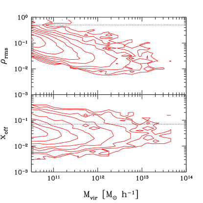
Figure 1: Correlation between the relaxedness parameters ($x_{\rm off}$ and $\rho_{\rm rms}$ and the virial mass $M_{\rm vir}$. The two dotted lines represents the limit values used to define ‘good’ haloes.

Following Macciò et al. (2007), we split our halo sample into unrelaxed and relaxed haloes. The latter are defined as the haloes with $\rho_{\rm rms}<0.5$ and $x_{\rm off}<0.07$. About 70% of the haloes in our sample qualify as relaxed haloes. In what follows, we will present results for two different samples of haloes: ‘all’, which includes all haloes with $N_{\rm vir}>1000$, and ‘good’ or ‘relaxed’, which is the corresponding subsample of relaxed haloes.

3 Principal Component Analysis

3.1 Introduction to PCA

Principal component analysis (PCA) is a type of multivariate (multidimensional) statistics. The goal of such an analysis is to find a suitable representation of multivariate data, where representation here means that we somehow transform the data so that its essential structure is made more visible or accessible. PCA belongs to the area of unsupervised learning, because the representation must be learned from the data itself without any external input from a supervising “teacher”.

PCA is a powerful technique that has been used in classification and dimensional reduction of large data sets, in order to decrease the complexity of the analysis. Each member of a data set (a dark matter halo, in our case) is defined by an “information vector”, an $n$-tuple of numbers (the halo’s relevant properties, in our case). PCA consists of de-correlating sets of vectors by performing rotations in the $n$-dimensional parameter space. The final result is a diagonal covariance matrix, with the eigenvalues representing the amount of information (in the sense of variance) stored in each eigenvector, which is called a principal component.

The principal components can be considered a set of basis vectors that optimally filter the information hidden in the data. If most of the variance in the original data can be accounted for by just a few of the components, we will have found a simpler description of the original data set. By convention, the first principal component corresponds to the largest eigenvalue, the second principal component corresponds to the second largest eigenvalue, and so on. A consequence of this definition is that the first principal component (PC) is a minimum distance fit to a line in the space of the original variables. The second PC is then a minimum distance fit to a line in the plane perpendicular to the first PC, and so on. Therefore, the properties that dominate the first PC are the properties that contain the largest amount of information and to some extent determine the values of the other properties. Typically the eigenvalue for a PC must be $\geq 1$ to be significant; less significant PCs tend to be dominated by noise (e.g., Connolly & Szalay 1999). In any case, the amount of variance that a PC accounts for is more meaningful than the precise value of its eigenvalue. If the data have high signal-to-noise, and if the data are not very incomplete, then the amount of variance of the first few PCs can be associated with ‘information’ contained in the data.

In astronomy, PCA applications in studies of multivariate distributions have been discussed in detail (Efstathiou & Fall 1984; Murtagh & Heck 1987). PCA methods have been used to study stellar, galaxy, and quasar spectra (e.g., Connolly et al. 1995; Bailer-Jones et al. 1998; Madgwick et al. 2003; Yip et al.  2004; Ferreras et al. 2006; Rogers et al. 2007; Chen et al. 2009; McGurk et al. 2010; Boroson & Lauer 2010), galaxy properties (e.g., Conselice 2006; Scarlata et al. 2007), and stellar populations and the Fundamental Plane (e.g., Faber 1973; Eisenstein et al. 2003; Woo et al. 2008). In a recent study, Bonoli & Pen (2009) analyzed the stochasticity of dark matter haloes, which quantifies the scatter in the correlation between halo and galaxy density fields.

PCA methods have not yet been exploited to analyze the properties of dark matter haloes. Considering the increasing size and resolution of numerical simulations, PCA is a useful tool to determine the relative importance of halo properties, and to determine how fundamental the masses of haloes are. The primary goal of this paper is to use PCAs to analyze a variety of halo properties, including those introduced in Section 2.

3.2 Applying PCAs to DM Haloes

Before we perform our principal component analyses on our simulation data, we subtract the mean from each halo property and normalize by the standard deviation. It follows that the distributions of the properties may be important: for example, choices about whether to take the logarithm of a property or whether to include objects whose properties are outliers in the distributions may be important. It is particularly useful to take the logarithm of halo mass, for example, because its range spans many orders of magnitude, and the spin parameter, because this makes its distribution more Gaussian; for consistency, however, we take the logarithms of all of the halo properties in our PCA. We also choose to exclude the extreme outliers ($>5\sigma$) in the distributions of properties. In addition, some properties are so strongly correlated that one property almost completely determines another (such as the virial mass, radius and velocity, or spin and angular momentum, or shape and triaxiality), and in such a case we include only what we believe is the more important property. By reducing the number of parameters, this tends to clarify the results of the PCA. We have performed numerous tests and have verified that these choices do not significantly affect our results.

We perform PCAs of each of the simulations described in Section 2. We analyze all of the haloes in each box, as well as the ‘relaxed’ haloes, with low values of $\rho_{\mathrm{rms}}$ (the r.m.s. of the NFW fit to the density profile) and $x_{\mathrm{off}}$ (the offset between the most bound particle and the center of mass).

The probability distributions of the halo properties are shown in Figure 2, for haloes in the 90 Mpc box, at fixed halo mass (see Section 4.2). By construction, PCA only finds independent normal processes, and works most effectively when the data set is jointly normally distributed. Our halo parameters are chosen to be approximately independent, and as can be seen in the figure, their distributions are approximately Gaussian. The shape parameter $q$ and the position angle $\Phi_{L}$ have slightly non-Gaussian distributions, with a tail of low values, but this is not sufficient to significantly affect the PCA results.

Figure 2: Distributions of halo properties at fixed mass (${\rm log}~{}(M/h^{-1}M_{\odot})\sim 12$), for haloes with more than 1000 particles in the high resolution 90 Mpc box. For a given property $x$, we define the mean-subtracted and standard deviation-normalized quantity as $x^{\prime}\equiv(x-{\bar{x}})/\sigma_{x}$.

property	median	mean	std dev
${\rm log}\,c_{\rm vir}$	1.043	1.039	0.107
${\rm log}\,\lambda$	-1.498	-1.513	0.252
${\rm log}\,q$	-0.101	-0.126	0.094
${\rm log}\,\Phi_{L}$	0.207	0.147	0.249
${\rm log}\,x_{\rm off}$	-1.614	-1.622	0.248
${\rm log}\,\rho_{\rm rms}$	-1.439	-1.413	0.259

Table 2: Median, mean, and standard deviation of halo properties at fixed mass in the 90 Mpc box, whose distributions are shown in Figure 2.

Lastly, we show the log halo mass distributions in Figure 3, for some of the analyses in Section 4. (In particular, these are the distributions for the PCAs whose results are shown in Tables 4, 6, 8, and 8.) We will perform PCAs with halo mass thresholds (Section 4.1), followed by PCAs at fixed halo mass (Section 4.2), and the mass distributions of some of these halo catalogues are shown in the figure. When a halo mass threshold is used, the mass distributions are highly non-Gaussian; nonetheless, the effect of this on the PCA results is minimal, as we discuss in the next section.

Figure 3: Log halo mass distributions for ${\rm log}~{}(M/h^{-1}M_{\odot})\geq 12$, 90 Mpc box (solid black histogram); ${\rm log}~{}(M/h^{-1}M_{\odot})\geq 12$, 180 Mpc box (long-dashed red histogram); relaxed haloes with $11.85\leq\mathrm{log}~{}(M/h^{-1}M_{\odot})<12.15$, 90 Mpc box (short-dashed black histogram); relaxed haloes with $13.2\leq\mathrm{log}~{}(M/h^{-1}M_{\odot})<13.5$, 180 Mpc box (dotted red histogram).

4 Results

For the principal component analyses, we focus on eight halo properties: mass, concentration, spin, shape, $\Phi_{L}$, $x_{\mathrm{off}}$, $\rho_{\mathrm{rms}}$, and overdensity. Firstly, in Section 4.1, we perform PCA of the haloes in our simulations using a halo mass threshold. Then in Section 4.2, we perform PCA at a fixed halo mass. Lastly, we briefly discuss the lack of a correlation between $\Phi_{L}$ and other halo parameters in Section 4.3.

4.1 PCAs with a halo mass threshold

The results of our principal component analyses of all of the haloes in the 90 and 180 Mpc boxes with ${\rm log}~{}(M/h^{-1}M_{\odot})\geq 12$ are shown in Tables 4 and 6; the results for the subset of relaxed haloes are shown in Tables 4 and 6. Similar PCA results for smaller and larger simulation boxes are shown in the appendix. Note that because of our resolution constraint, in the 180 Mpc box, most of the haloes with ${\rm log}~{}(M/h^{-1}M_{\odot})\geq 12$ are more massive than $10^{12.3}h^{-1}M_{\odot}$ (see Fig. 3).

We consider the following seven halo properties, of which we use the logarithms: the mass ($M_{\mathrm{vir}}$), the concentration ($c_{\mathrm{vir}}$), the spin ($\lambda$), the shape ($q$), the angle between the major axis and the total angular momentum ($\Phi_{L}$), $\rho_{\mathrm{rms}}$, and $x_{\mathrm{off}}$. We have performed tests of the uncertainties of the PCAs with bootstrap techniques and have found that our errors are extremely small; hence, we have omitted them from the tables, for clarity. In addition, our results are not significantly dependent on the selection criteria (i.e., the choice of the halo mass threshold, and for the PCAs later in this section, the particle limit and the $x_{\mathrm{off}}$ and $\rho_{\mathrm{rms}}$ criteria).

One striking result is the lack of a single or pair of dominant principal components. The first two principal components usually account for only about 40-50% of the variance. In contrast, in PCAs of galaxy spectra, the first one or two PCs usually dominate (e.g., Connolly et al. 1995; Madgwick et al. 2003). Recall that, as stated in Section 3.1, the later PCs (with lower eigenvalues) tend to be dominated by noise.

For dark matter haloes, no parameter or combination of parameters strongly determine the other parameters. (This is partly by construction, because for closely related parameters, like mass and radius or shape and triaxiality, we have included only one of the parameters.) In other words, although halo properties are correlated with each other, we find no clearly fundamental correlation (nor a fundamental ‘plane’).

This is also evident in Figure 4, in which the first two PCs of all haloes in the 90 Mpc box (Table 4) are shown. Some structure is apparent in the figure, with relaxed and unrelaxed haloes exhibiting different distributions. The figure illustrates that the relaxed haloes have larger values of PC1 (which is anti-correlated with the relaxedness parameters), and the fact that most haloes have $\mathrm{PC}2>-2$ is simply due to the halo mass threshold.

The PCA results of the different simulations are similar, but not equivalent, most likely because of the different ranges of halo masses. In any case, in the majority of our simulation boxes, combinations of $M_{\mathrm{vir}}$, $c_{\mathrm{vir}}$, $x_{\mathrm{off}}$, and $\rho_{\mathrm{rms}}$ dominate the first two principal components. Halo mass and concentration, on the one hand, and halo relaxedness, on the other, can explain at least half of the variance. Note, however, that halo mass is never significant on the first PC. $x_{\mathrm{off}}$ and $\rho_{\mathrm{rms}}$ indicate the relaxedness of haloes, and for unrelaxed haloes, the concentration is not well-defined. Therefore, we argue that the relaxedness of haloes is at least as important as their mass and concentration for determining halo properties. This is the primary result of our paper.

property	PC 1	PC 2	PC 3	PC 4
${\rm log}\,M_{\rm vir}$	0.103	-0.761	0.148	0.500
${\rm log}\,c_{\rm vir}$	-0.555	0.156	-0.015	-0.134
${\rm log}\,\lambda$	0.369	0.009	0.062	-0.333
${\rm log}\,q$	0.094	0.579	0.143	0.759
${\rm log}\,\Phi_{L}$	0.001	-0.059	-0.971	0.181
${\rm log}\,x_{\rm off}$	0.547	-0.018	-0.012	-0.041
${\rm log}\,\rho_{\rm rms}$	0.488	0.240	-0.107	-0.105
eigenvalues	2.56	1.18	1.01	0.90
% of variance	36.5%	16.9%	14.4%	12.8%

Table 3: All haloes with ${\rm log}~{}(M/h^{-1}M_{\odot})\geq 12$, 90 Mpc box, high resolution. $N$=2183.

property	PC 1	PC 2	PC 3	PC 4
${\rm log}\,M_{\rm vir}$	0.163	-0.762	0.064	0.166
${\rm log}\,c_{\rm vir}$	-0.604	0.231	0.006	-0.114
${\rm log}\,\lambda$	0.392	0.102	0.128	-0.221
${\rm log}\,q$	0.085	0.307	0.304	0.887
${\rm log}\,\Phi_{L}$	0.033	-0.025	-0.928	0.300
${\rm log}\,x_{\rm off}$	0.543	-0.001	0.021	-0.047
${\rm log}\,\rho_{\rm rms}$	0.389	0.511	-0.162	-0.176
eigenvalues	1.84	1.35	1.01	0.96
% of variance	26.3%	19.2%	14.5%	13.7%

Table 4: ‘Good’ (relaxed) haloes with ${\rm log}~{}(M/h^{-1}M_{\odot})\geq 12$, 90 Mpc box, high resolution. $N$=1701.

property	PC 1	PC 2	PC 3	PC 4
${\rm log}\,M_{\rm vir}$	0.480	0.467	0.025	-0.078
${\rm log}\,c_{\rm vir}$	0.221	-0.639	-0.022	0.007
${\rm log}\,\lambda$	-0.320	0.417	-0.033	0.046
${\rm log}\,q$	-0.218	-0.023	0.263	-0.936
${\rm log}\,\Phi_{L}$	0.013	0.001	0.963	0.268
${\rm log}\,x_{\rm off}$	-0.539	0.257	-0.040	0.167
${\rm log}\,\rho_{\rm rms}$	-0.530	-0.358	-0.011	0.126
eigenvalues	1.94	1.64	1.00	0.95
% of variance	27.7%	23.5%	14.3%	13.6%

Table 5: All haloes with ${\rm log}~{}(M/h^{-1}M_{\odot})\geq 12$, 180 Mpc box. $N$=6391.

property	PC 1	PC 2	PC 3	PC 4
${\rm log}\,M_{\rm vir}$	-0.618	-0.098	0.030	0.011
${\rm log}\,c_{\rm vir}$	0.443	-0.469	-0.003	0.044
${\rm log}\,\lambda$	-0.062	0.664	-0.044	-0.012
${\rm log}\,q$	0.113	0.286	0.404	0.802
${\rm log}\,\Phi_{L}$	0.010	-0.004	0.899	-0.435
${\rm log}\,x_{\rm off}$	0.236	0.494	-0.164	-0.406
${\rm log}\,\rho_{\rm rms}$	0.591	0.066	0.002	-0.008
eigenvalues	2.06	1.25	1.01	0.98
% of variance	29.4%	17.8%	14.4%	14.0%

Table 6: ‘Good’ (relaxed) haloes with ${\rm log}~{}(M/h^{-1}M_{\odot})\geq 12$, 180 Mpc box. $N$=3757.

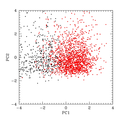
Figure 4: First two principal components plotted against each other, for all haloes with ${\rm log}~{}(M/h^{-1}M_{\odot})\geq 12$ in the 90 Mpc box. We are using the results from the first two columns of Table 4: for example, for a given halo, PC1$=-0.103\,(\mathrm{log}\,M_{\mathrm{vir}})^{\prime}+0.555\,(\mathrm{log}\,c_{\mathrm{vir}})^{\prime}-0.369\,(\mathrm{log}\,\lambda)^{\prime}-0.094\,(\mathrm{log}\,q)^{\prime}-0.001\,(\mathrm{log}\,\Phi_{L})^{\prime}-0.547\,(\mathrm{log}\,x_{\mathrm{off}})^{\prime}-0.488\,(\mathrm{log}\,\rho_{\mathrm{rms}})^{\prime}$, where the halo parameters are mean-subtracted and normalized by the standard deviation. The red points are the subset of ‘good’ (i.e., relaxed) haloes.

When halo parameters appear together on a PC, this can indicate a correlation between those parameters. For example, when a PC is dominated by mass and concentration, they usually have opposite signs, consistent with the fact that these halo properties are anti-correlated (e.g., Bullock et al. 2001). Correlated halo properties do not necessarily dominate the same PCs, however, and properties dominating a PC are not necessarily correlated, although this is often the case. If two correlated properties have substantial scatter between them, or if their correlation is due to more fundamental correlations with a third parameter, or if two properties have strongly correlated errors, the interpretation of PCA results may be more complicated. With our choice of halo properties and selection criteria, we have attempted to minimize these complications.

Finally, note the similarities and differences between the results for all haloes and for just the relaxed haloes. Most of the same halo parameters dominate the first few principle components. In addition, the PCA results are mostly similar in the different resolution simulation boxes, indicating that our results are not very sensitive to resolution, though the significance of the spin parameter varies slightly. Although we find that the PCA results presented here are statistically stable, in some cases the first PC of one simulation box resembles the second PC of another, and vice versa, suggesting that it is the combination of the first two PCs that is important. In any case, throughout our analyses, halo mass and concentration on the one hand, and relaxedness parameters (quantified by $x_{\mathrm{off}}$ and $\rho_{\mathrm{rms}}$) on the other, continue to dominate the first two PCs.

We also note that the halo mass distributions are non-Gaussian when a mass threshold is used (Fig. 3), and this could potentially affect the PCA results. We have tested this effect by performing PCAs with subsamples that have Gaussian mass distributions, and by PCAs with the whole samples but with the mass distributions rescaled (forcing them to be Gaussian, with the same rank order), and we find that the results are virtually the same, differing from Tables 4-6 by $<1\%$.

Nonetheless, some halo parameters are accurately determined only for relaxed haloes (Macciò et al. 2007), such that the very unrelaxed haloes introduce noise in the other parameters and could relegate them to the later PCs, or could introduce artificial correlations with the relaxedness parameters. For these reasons, for the rest of this paper, we focus on PCA results based on the subset of relaxed haloes.

4.2 PCAs at fixed halo mass

As shown in Figure 2, at fixed halo mass, the distributions of the logarithm of most halo properties are approximately Gaussian (i.e., $p(\mathrm{log}\,\lambda|M)$, $p(\mathrm{log}\,c|M)$, etc., can be fit fairly well by Gaussian distributions). It therefore makes sense to perform PCAs of these variates at fixed mass. Constraints from these PCAs could be useful for halo model analyses (e.g., of galaxy clustering, weak lensing, galaxy groups and clusters), and perhaps for semi-analytic models as well, because they reduce the complexity of such analyses to a Gaussian Mixture model. Gaussian Mixture models have a well developed statistical framework and have been applied to a variety of astrophysical studies (e.g., Kelly & McKay 2004; Hao et al. 2009; Skibba & Sheth 2009).

We first perform PCAs similar to those in Section 4.1, but now at fixed halo mass, using the other six halo parameters. The results of these PCAs are shown in Table 8 for haloes with $11.85\leq\mathrm{log}~{}(M/h^{-1}M_{\odot})<12.15$ in the 90 Mpc box, and in Table 8 for haloes with $13.2\leq\mathrm{log}~{}(M/h^{-1}M_{\odot})<13.5$ in the 180 Mpc box. Only haloes with more than 1000 particles are included.

property	PC 1	PC 2	PC 3	PC 4
${\rm log}\,c_{\rm vir}$	-0.601	-0.076	0.044	-0.011
${\rm log}\,\lambda$	0.441	-0.089	0.544	-0.048
${\rm log}\,q$	0.167	-0.591	-0.427	-0.654
${\rm log}\,\Phi_{L}$	-0.023	0.772	-0.113	-0.605
${\rm log}\,x_{\rm off}$	0.552	0.088	0.158	-0.071
${\rm log}\,\rho_{\rm rms}$	0.334	0.183	-0.694	0.446
eigenvalues	1.79	1.06	0.97	0.93
% of variance	29.8%	17.6%	16.2%	15.4%

Table 7: ‘Good’ (relaxed) haloes with ${\rm log}~{}(M/h^{-1}M_{\odot})\sim 12$ and more than 1000 particles, 90 Mpc box, high resolution. $N$=1056.

property	PC 1	PC 2	PC 3	PC 4
${\rm log}\,c_{\rm vir}$	-0.643	0.107	0.015	0.000
${\rm log}\,\lambda$	0.496	0.141	0.339	0.120
${\rm log}\,q$	0.181	-0.567	-0.389	-0.642
${\rm log}\,\Phi_{L}$	0.052	-0.588	0.715	0.058
${\rm log}\,x_{\rm off}$	0.520	0.058	-0.353	0.344
${\rm log}\,\rho_{\rm rms}$	-0.186	-0.546	-0.313	0.672
eigenvalues	1.55	1.13	0.97	0.93
% of variance	25.8%	18.8%	16.2%	15.6%

Table 8: ‘Good’ (relaxed) haloes with ${\rm log}~{}(M/h^{-1}M_{\odot})\sim 13.35$ and more than 1000 particles, 180 Mpc box. $N$=416.

The results are similar to those of the previous section, with concentration and $x_{\mathrm{off}}$ dominating the first principal component, although the spin parameter is now important on this PC as well. In addition, $\Phi_{L}$ and the shape parameter dominate the second PC. Halo model analyses often involve constructing mock galaxy catalogues, and the models are often based on the clustering and abundance of haloes as a function of their masses; at fixed mass, the models use halo concentrations and density profiles. Perhaps the models could also use halo spin distributions, to more accurately describe galaxy velocities, as well as $x_{\mathrm{off}}$ distributions, to describe central galaxies offset from the halo centers.

Next, we perform PCAs with an additional parameter, the overdensity $\Delta_{8}$ within a sphere of radius 8 Mpc, which is an indicator of a halo’s local environment (since the largest haloes have virial radii of $\sim 2\,\mathrm{Mpc}/h$). At a fixed halo mass, there may be a range of environments: some haloes may be embedded within large structures or filaments or surrounded by infalling haloes, while some may be relatively isolated (e.g., Colberg et al. 1999). Using a fixed halo mass also ensures that the haloes are of similar size and are much smaller than the density aperture. We have restricted this analysis to haloes with more than 1000 particles and with $13.15<\mathrm{log}~{}(M/h^{-1}M_{\odot})<13.45$ in the 180 Mpc box and $13.45<\mathrm{log}~{}(M/h^{-1}M_{\odot})<13.75$ in one of the 300 Mpc boxes. It is useful to analyze the haloes in a large simulation box, in which cosmic variance is relatively unimportant.

property	PC 1	PC 2	PC 3	PC 4
${\rm log}\,\Delta_{8}$	-0.252	-0.103	0.761	-0.036
${\rm log}\,c_{\mathrm{vir}}$	0.630	0.059	0.247	0.049
${\rm log}\,\lambda$	-0.499	-0.054	0.123	0.226
${\rm log}\,q$	-0.126	-0.585	0.115	-0.667
${\rm log}\,\Phi_{L}$	-0.007	-0.595	-0.495	0.159
${\rm log}\,x_{\mathrm{off}}$	0.509	0.205	-0.149	0.187
${\rm log}\,\rho_{\mathrm{rms}}$	0.128	-0.494	0.256	0.664
eigenvalues	1.51	1.10	1.02	0.97
% of variance	21.6%	15.7%	14.6%	13.8%

Table 9: ‘Good’ (relaxed) haloes with ${\rm log}~{}(M/h^{-1}M_{\odot})\sim 13.3$ and more than 1000 particles, 180 Mpc box. $N$=383.

property	PC 1	PC 2	PC 3	PC 4
${\rm log}\,\Delta_{8}$	-0.138	-0.164	0.819	0.418
${\rm log}\,c_{\mathrm{vir}}$	0.629	0.051	0.112	-0.061
${\rm log}\,\lambda$	-0.521	-0.050	0.095	0.138
${\rm log}\,q$	-0.050	0.603	0.249	-0.149
${\rm log}\,\Phi_{L}$	0.093	0.405	-0.347	0.840
${\rm log}\,x_{\mathrm{off}}$	-0.544	0.256	-0.206	-0.183
${\rm log}\,\rho_{\mathrm{rms}}$	0.084	0.613	0.288	-0.203
eigenvalues	1.50	1.11	1.02	0.96
% of variance	21.5%	15.9%	14.6%	13.8%

Table 10: ‘Good’ (relaxed) haloes with ${\rm log}~{}(M/h^{-1}M_{\odot})\sim 13.6$ and more than 1000 particles, 300 Mpc box. $N$=944.

We find that the local overdensity is usually significant on the third principle component, where it is sometimes paired with the angle $\Phi_{L}$. This is consistent with Altay et al. (2006), who found that haloes are aligned with their large-scale structures (if they are located in filaments, for example), while halo shapes are not dependent on membership of a filament. It is also consistent with Wang et al. (2011), who showed that a halo’s spin is correlated with the local overdensity and the strength of the tidal field. In any case, in all of our simulations, the density is rarely significant on the first two PCs. Therefore, we argue that, at fixed mass, a halo’s environment is relatively unimportant, because it does not significantly determine the halo’s properties. At fixed mass, a halo’s angular momentum and degree of relaxedness are much more important.

4.3 Correlation with $\Phi_{L}$

As previously stated the angle $\Phi_{L}$ can be thought of as a proxy for the position of a possible stellar disk within the dark matter halo, assuming an alignment between the angular momentum of the dark matter particle and the stellar component (e.g., Hahn et al. 2010). Figure 5 shows the probability distribution of the cosine of $\Phi_{L}$ in the high resolution 90 Mpc box. In the upper panel the angle $\Phi_{L}$ is defined as the angle between the minor axis and the angular momentum $L$, while in the lower panel the major axis is used. For relaxed haloes the probability distribution is remarkably flat in both cases, and there is no sign of a possible alignment between either the major or minor axis and $L$. If we restrict our analysis to high spin haloes ($\lambda>0.07$, red dashed line, $\approx 12\%$ of the total) a weak maximum at $\cos(\Phi_{L})=0$ arises for the angle with the major axis, while there is still no evidence for a correlation between the orientation of the minor axis and the halo angular momentum.

This result is consistent with Zentner et al. (2005b) and Kuhlen et al. (2007), who showed that subhaloes are distributed anisotropically and are preferentially aligned with the major axis of the triaxial halo. Studies of satellite galaxies in groups have reached similar conclusions (Yang et al. 2006; Faltenbacher et al. 2007; Kang et al. 2007; Wang et al. 2008). Nonetheless, other studies have detected significant correlations between the spin axis of haloes and their minor axis, stronger than correlations with the major axis (Bailin & Steinmetz 2005; Bett et al. 2007). It is possible that the disagreement between our result (Fig. 5) and these studies somehow owes to the differences between SO and friends-of-friends (FOF) halo-finding algorithms. As noted by a number of authors, there are different disadvantages to these two types of halo-finders (e.g., Bett et al. 2007; Tinker et al. 2008b; Knebe et al. 2011). In particular, SO halo-finders tend to impose a more spherical geometry on the resulting systems. On the other hand, FOF halo-finders often identify objects linked with neighboring objects via tenuous bridges of particles, resulting in anomolously large velocity dispersions, masses, and spin parameters of $\approx 6\%$ of objects (Bett et al. 2007). In addition, FOF halo-finders define a halo center as the center-of-mass, while most other algorithms (including ours) define the center as the center of the density profile (i.e., the most bound particle) (Knebe et al. 2011). These differences with FOF halo-finders may explain the disagreement about correlations between the spin axis and major or minor axes of haloes.

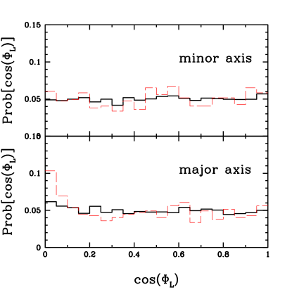
Figure 5: Probability distribution for the angle $\Phi_{L}$ between the angular momentum vector $L$ and the minor (upper panel) and major (lower panel) axis of the dark matter distribution. The solid black line is for relaxed haloes in the 90 Mpc box, while the red line is for the spin haloes ($\lambda>0.07$, $\approx 12\%$ of the total).

Returning to our PCA results, in the different simulation boxes, rarely does a single halo parameter dominate a particular principle component. Nonetheless, $\Phi_{L}$ usually dominates the third or fourth PC, although sometimes the shape parameter is also significant on the same PC. In other words, one might interpret this as evidence that $\Phi_{L}$ is weakly correlated with spin and/or shape, but not related to other halo properties. $\Phi_{L}$, which is the angle between the major axis of the halo and its angular momentum vector, is expected to be important for the formation of disk galaxies, because the angular momenta of the stellar disk and the dark matter particles are generally, though not always, expected to be aligned (van den Bosch et al. 2002; Kazantzidis et al. 2004; Zentner et al. 2005b; Sharma & Steinmetz 2005; Bett et al. 2010; Hahn et al. 2010).

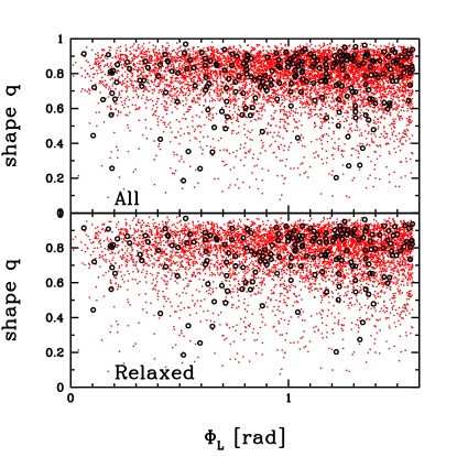
Figure 6: Relation between the shape ($q$) and the angle $\Phi_{L}$. Black circle and red dots represent haloes from the W5-30.1 and the W5-90.2 simulations, respectively. The two panel shows results for All (upper) and Relaxed haloes. In both cases there is no correlation between the two properties.

In contrast to this, we show in Figure 6 that $\Phi_{L}$ is uncorrelated with the shape parameter $q$. This result is independent of the value of the angular momentum (quantified by the spin parameter) as shown in Figure 7. Therefore, as a consequence of our results, we argue that it is not possible to reliably determine the angle of the angular momentum vector from a halo’s shape. This has consequences for the formation of disk galaxies, which we discuss in the final section of the paper.

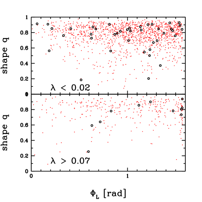
Figure 7: Same as Figure 6 but of haloes with different spins. The upper panel shows results for relaxed haloes with little angular momentum (defined as haloes with $\lambda<0.02$) while the lower one is for relaxed haloes with a lot of angular momentum ($\lambda>0.07$). Again, there is no correlation between spin ($\lambda$) and the angle $\Phi_{L}$.

5 Dependence on Halo Relaxedness

From the results of the PCAs in Sections 4.1 and 4.2, we argued that halo ‘relaxedness’ is as important as halo mass in determining halo properties, because mass and relaxedness account for the majority of the variance in the PCAs. This conclusion about the importance of halo relaxedness is consistent with other studies, such as Shaw et al. (2006), who find that the dynamical state of haloes, quantified by the virial ratio, is correlated with halo parameters: mass, concentration, spin as well as the substructure fraction. In addition, Neto et al. (2007) define an ‘equilibrium state’ in terms of the substructure fraction, center of mass displacement (like our $x_{\mathrm{off}}$), and virial ratio, and find that a halo’s equilibrium state is correlated with its mass, concentration, and spin.

In order to investigate this issue further, in this section we quantify and compare correlations between halo properties and mass, and between them and the relaxedness parameters.

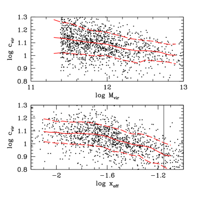
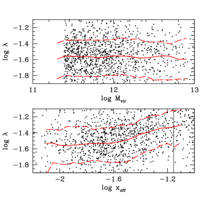
Figure 8: Left: $M_{\mathrm{vir}}$ vs $c_{\mathrm{vir}}$ for very relaxed haloes ($x_{\mathrm{off}}<0.018$, $\rho_{\mathrm{rms}}<0.14$) in the upper panel, and $x_{\mathrm{off}}$ vs $c_{\mathrm{vir}}$ at fixed mass ($11.85\leq\mathrm{log}~{}(M/h^{-1}M_{\odot})<12.15$, as in Section 4.2) in the lower panel, for haloes with more than 1000 particles in the 90 Mpc box. Right: same, but with the spin parameter, $\lambda$. Points indicate individual haloes, solid lines show the running medians, and dashed lines show the 16 and 84 percentiles. The vertical lines in the lower panels indicate our cut for relaxed haloes, at $x_{\mathrm{off}}<0.07$.

In particular, we first perform Spearman rank tests on some correlations between these parameters. We begin with correlations with halo relaxedness parameters at fixed mass ($11.85\leq\mathrm{log}~{}(M/h^{-1}M_{\odot})<12.15$), using haloes with more than 1000 particles in the 90 Mpc box. This is one of the catalogues used in Section 4.2 (see PCA result in Table 8). The correlations between concentration and $x_{\mathrm{off}}$, and between spin and $x_{\mathrm{off}}$ are statistically significant, with Spearman ranks $r_{s}=-0.65$ and $0.42$, respectively, and remain significant if only ‘good’ (i.e., relaxed) haloes are selected. The correlation with shape is weaker, while that with $\Phi_{L}$ is not significant at all. Of the correlations with $\rho_{\mathrm{rms}}$, only that with concentration is significant, with $r_{s}=-0.45$. Therefore, the dependence on relaxedness at fixed mass is predominantly due to $x_{\mathrm{off}}$.

In order to perform a fair comparison with the halo mass dependence, we test the strength of correlations with mass at fixed relaxedness: we use the same simulation box and select haloes within a narrow range of relaxedness parameters ($x_{\mathrm{off}}<0.018$ and $\rho_{\mathrm{rms}}<0.14$), such that there are a similar number of haloes ($\sim 1300$) as the previous test at fixed mass. Only the resulting mass-concentration correlation is still significant, with $r_{s}=-0.38$. These results imply that the expected weak correlations between mass and the spin parameter, and between mass and shape (e.g., Macciò et al. 2007; Bett et al. 2007), are no longer significant once one accounts for the dependence on halo relaxedness.

In Figure 8, we show some of these correlations that we tested with the Spearman rank coefficients. In the left panels of Figure 8, we show the correlation between concentration and $x_{\mathrm{off}}$ at fixed mass, and compare it to the mass-concentration relation at fixed relaxedness parameters (similar to Fig. 2 of Macciò et al. (2008)). Halo mass and the center of mass offset appear to be independently correlated with concentration (i.e., one is not due to the other). More massive haloes and haloes with larger offsets tend to be less concentrated.

We show the analogous plots with the spin parameter $\lambda$ in the right panels of Figure 8. One can see no mass dependence at fixed relaxedness, although at fixed mass, haloes with larger offsets $x_{\mathrm{off}}$ tend to have larger spin. Although the spin parameter is not well-defined for unrelaxed haloes, we see that the correlation occurs for haloes defined as relaxed (with $\mathrm{log}~{}x_{\mathrm{off}}<-1.15$, or the stricter criterion in Macciò et al. (2007), $\mathrm{log}~{}x_{\mathrm{off}}<-1.40$).

These tests show that halo concentration and spin are as tightly correlated with the relaxedness parameters (especially $x_{\mathrm{off}}$) as with halo mass. This confirms our conclusion that the relaxed state of a halo is as important as its mass, in determining its other properties.

6 Discussion and conclusions

We used numerical simulations of dark matter haloes to study a variety of halo properties: mass, concentration, spin, shape, the angle between the major axis and the angular momentum vector ($\Phi_{L}$), the distance between the most bound particle and the centre of mass ($x_{\mathrm{off}}$), the r.m.s. of the NFW fit to the density profile ($\rho_{\mathrm{rms}}$), and the local overdensity. We analyzed all of these properties together, by employing principal component analysis (PCA).

We summarize our main results as follows:

• There is no single dominant PC or pair of PCs. Unlike the spectra of galaxies, for dark matter haloes, there is no parameter or combination of parameters that strongly determine the other parameters..

• We find that whether a halo is relaxed or not is at least as important as the halo’s mass and concentration. Even for relatively relaxed haloes, the degree of relaxedness, quantified by $x_{\mathrm{off}}$ and $\rho_{\mathrm{rms}}$, is still as important as mass and concentration, and these four properties tend to dominate the first two principal components.

• $\Phi_{L}$ is not significantly correlated with any other halo properties. It is therefore not possible to reliably estimate the direction of the angular momentum vector of a halo from its shape.

• A halo’s ‘environment’ (quantified by the 8 Mpc overdensity) usually dominates the third principle component, where it is sometimes combined with the angle $\Phi_{L}$, but it is less significant than other halo properties on the first two principle components. Therefore, at fixed halo mass, the environment is relatively unimportant in determining the other halo properties.

Our results have many important implications, especially for halo occupation models and semi-analytic models. Most such models explicitly assume that halo mass (or the combination of mass and concentration) largely determines other important halo properties, and to some extent determines the properties of the galaxies hosted by a halo; however, our results show that this assumption is often false: halo mass is less dominant than one might expect. The degree of relaxedness of a halo is at least as important as its mass. Therefore, the relaxedness of a halo could affect the formation of galaxies hosted by it, independent of halo mass. In an unrelaxed halo, for example, galaxies may experience stronger tidal forces or their supply of gas to form stars could be disrupted. For semi-analytic models, one solution may be to quantify the relaxedness of the dark matter haloes and to use them in addition to the halo merger histories. For halo occupation models, it is possible that the unrelaxedness of some haloes may affect or blur the relation between halo mass and central galaxy luminosity or stellar mass. In addition, it is possible that the halo mass function and halo mass-concentration relation assumed in the models could be different for relaxed and unrelaxed haloes. It is not yet clear how strongly halo relaxedness may affect results from halo occupation and semi-analytic models, and these issues deserve further study.

A related issue is that of halo ‘assembly bias’, in which the formation time of haloes (or other properties related to halo assembly) is correlated with the environment at fixed mass (e.g., Sheth & Tormen 2004; Croton, Gao & White 2007; Wetzel et al. 2007; Faltenbacher & White 2010; Fakhouri & Ma 2010). The relaxedness of haloes, which we quantify with $\rho_{\rm rms}$ and $x_{\rm off}$, is clearly related to their assembly: a halo that has recently formed or recently experienced a merger is more likely to be unrelaxed. Although our density parameter, $\Delta_{8}$ is subdominant in our PCAs, it is nonetheless possible that the relaxedness of haloes is related to their larger scale environment. Hence, the correlations with halo relaxedness may be a manifestation of halo assembly bias. Nonetheless, assembly bias may have a relatively weak effect for halo models of galaxy clustering (e.g., Blanton & Berlind 2007; Tinker et al. 2008a; Skibba & Sheth 2009).

Our result for the angle $\Phi_{L}$ also has interesting implications. The fact that $\Phi_{L}$ is not significantly correlated with other halo properties may present a difficulty for some models. While the angular momentum of the stellar disk of a galaxy is thought to be aligned with the dark matter particles of the host halo (such that the pole of the disk is collinear with the angular momentum vector of the halo), our result implies that it is actually quite difficult, if not impossible, to accurately determine the orientation of the disk simply by looking at the halo’s shape. This is consistent with hydrodynamical simulations that include baryonic cooling, which result in disks with spin axes that are very poorly aligned with the halo (Bailin et al. 2005). It suggests that the direction of the angular momentum of the baryons is not well conserved throughout the disk formation process (van den Bosch et al. 2002; Yang et al. 2006). Heller et al. (2007) also argue that the shape and morphology of a disk depend on the relative angle with the major axis of the halo, but this dependence too is not well conserved. Therefore, although the formation of disk galaxies and their host halos are certainly related, after they have evolved, it is not clear that one could reliably determine to what extent the disk remains aligned with the halo.

Finally, at the time of publication, Jeeson-Daniel et al. (2011) posted a preprint of a related study, involving PCAs of various halo properties. Some of the results in Jeeson-Daniel et al. are consistent with ours, such as that halo mass, concentration, substructure, and relaxedness are among a set of parameters that together account for a large fraction of the variance. Nonetheless, their relaxedness parameter, which is similar to our $x_{\rm off}$, accounts for less variance in their PCAs than in ours.

Appendix A Supplementary PCAs and Tests

In this appendix, we include additional principle component analyses that can be compared to the results in Section 4.

Firstly, we perform PCAs for halo mass threshold ($\mathrm{log}~{}(M/h^{-1}M_{\odot})>12$) for the 40 and 300 Mpc simulation boxes, analogous to the results shown in Tables 4 and 6. The results of these PCAs are shown in Tables 12 and 12. The PCAs of the 40 and 90 Mpc boxes are similar, although for the 40 Mpc box, $\lambda$ is now very significant on the second PC. The PCAs of the 180 and 300 Mpc boxes are similar as well, although for the 300 Mpc box, $c_{\mathrm{vir}}$ is more significant on the first PC than on the second one. In any case, even when one compares the PCAs of the 40 and 300 Mpc boxes, which have very different resolutions, the results are quite similar. We conclude that our results are not very sensitive to the resolution of the simulations.

property	PC 1	PC 2	PC 3	PC 4
${\rm log}\,M_{\rm vir}$	-0.618	0.078	-0.002	0.015
${\rm log}\,c_{\mathrm{vir}}$	0.408	0.499	-0.015	0.078
${\rm log}\,\lambda$	-0.068	-0.645	-0.046	-0.070
${\rm log}\,q$	0.093	-0.267	0.458	0.820
${\rm log}\,\Phi_{L}$	0.002	-0.053	-0.881	0.467
${\rm log}\,x_{\mathrm{off}}$	0.292	-0.503	-0.106	-0.313
${\rm log}\,\rho_{\mathrm{rms}}$	0.595	-0.046	-0.014	-0.022
eigenvalues	2.14	1.26	1.01	0.97
% of variance	30.6%	18.0%	14.4%	13.9%

Table 11: Relaxed haloes with ${\rm log}~{}(M/h^{-1}M_{\odot})\geq 12$, 40 Mpc box. $N$=1822.

property	PC 1	PC 2	PC 3	PC 4
${\rm log}\,M_{\rm vir}$	-0.460	0.472	-0.124	-0.003
${\rm log}\,c_{\mathrm{vir}}$	0.609	0.185	0.045	-0.009
${\rm log}\,\lambda$	-0.338	-0.465	0.116	0.044
${\rm log}\,q$	0.075	-0.367	-0.360	-0.818
${\rm log}\,\Phi_{L}$	0.112	-0.161	-0.862	0.463
${\rm log}\,x_{\mathrm{off}}$	-0.312	-0.483	0.136	0.240
${\rm log}\,\rho_{\mathrm{rms}}$	0.434	-0.364	0.279	0.239
eigenvalues	1.62	1.33	0.99	0.96
% of variance	23.2%	19.0%	14.2%	13.7%

Table 12: Relaxed haloes with ${\rm log}~{}(M/h^{-1}M_{\odot})\geq 12$ and more than 1000 particles, 300 Mpc box. $N$=1905.

Next, we perform more PCAs at fixed mass, using smaller-scale overdensities $\Delta_{2}$ and $\Delta_{4}$, in 2 and 4 Mpc apertures, analogous to the results in Table 10. The results of these PCAs are shown in Tables 14 and 14. When using $\Delta_{4}$, the first three PCs are essentially the same as when $\Delta_{8}$ was used, and $q$ still dominates the fourth PC. When $\Delta_{2}$ is used, the second and third PCs are different, although they are dominated by the same parameters. In any case, regardless of the scale of the overdensity, we conclude that halo environment is less prominent in our PCAs, and therefore less important, than the other halo parameters.

property	PC 1	PC 2	PC 3	PC 4
${\rm log}\,\Delta_{2}$	0.282	0.406	0.559	0.031
${\rm log}\,c_{\mathrm{vir}}$	-0.621	0.221	0.150	-0.023
${\rm log}\,\lambda$	0.511	0.035	0.181	-0.290
${\rm log}\,q$	0.098	-0.542	0.201	0.755
${\rm log}\,\Phi_{L}$	-0.023	-0.688	0.084	-0.580
${\rm log}\,x_{\mathrm{off}}$	0.505	0.061	-0.201	0.062
${\rm log}\,\rho_{\mathrm{rms}}$	-0.098	-0.118	0.738	-0.070
eigenvalues	1.52	1.11	1.08	0.97
% of variance	21.8%	15.8%	15.4%	13.8%

Table 13: Relaxed haloes with ${\rm log}~{}(M/h^{-1}M_{\odot})\sim 13.3$ and more than 1000 particles, 180 Mpc box. $N$=383.

property	PC 1	PC 2	PC 3	PC 4
${\rm log}\,\Delta_{4}$	0.233	-0.181	0.751	0.049
${\rm log}\,c_{\mathrm{vir}}$	-0.626	0.024	0.303	-0.024
${\rm log}\,\lambda$	0.502	-0.066	0.157	-0.271
${\rm log}\,q$	0.124	-0.569	-0.110	0.772
${\rm log}\,\Phi_{L}$	0.131	-0.572	-0.442	-0.470
${\rm log}\,x_{\mathrm{off}}$	0.521	0.200	-0.006	-0.037
${\rm log}\,\rho_{\mathrm{rms}}$	-0.123	-0.521	0.336	-0.325
eigenvalues	1.51	1.10	1.03	0.97
% of variance	21.6%	15.7%	14.7%	13.8%

Table 14: ‘Good’ (relaxed) haloes with ${\rm log}~{}(M/h^{-1}M_{\odot})\sim 13.3$ and more than 1000 particles, 180 Mpc box. $N$=383.

Finally, while we have attempted to minimize the effects of correlated errors, we have not heretofore accounted for parameters with particularly large errors. One way to test the effects of such errors is to add error (with a Gaussian distribution) to a particular parameter. Such tests yield PCA results similar to those shown in Section 4, although we find that the first few principal components are usually more robust than the later PCs. An example is shown in Table 15, in which we have significantly increased the error of the spin parameter, by 1-$\sigma$. Comparing to Table 10, the numbers are slightly different, but the dominant parameters on each PC remain the same. The only exception is $\lambda$ itself, which is no longer significant on PC 1, but is instead slightly significant on PC 2 and more significant on PC 4. Similar tests with other parameters have yielded smaller changes than shown here: for example, adding error to the concentration does not affect any of the dominant parameters on the PCs, and only slightly decreases $c_{\mathrm{vir}}$’s significance on PC 1. We have also tested the effects of asymmetric errors, but these significantly affect the PCA results only if they are larger and much more asymmetric than the expected errors in these simulations. We conclude that our PCA results are robust to the parameter errors.

property	PC 1	PC 2	PC 3	PC 4
${\rm log}\,\Delta_{8}$	0.249	0.100	0.762	0.210
${\rm log}\,c_{\mathrm{vir}}$	-0.663	0.022	0.195	0.176
${\rm log}\,\lambda$	0.282	0.367	-0.020	0.639
${\rm log}\,q$	0.186	0.428	0.251	-0.713
${\rm log}\,\Phi_{L}$	0.034	0.623	-0.504	0.034
${\rm log}\,x_{\mathrm{off}}$	0.602	-0.245	-0.084	0.043
${\rm log}\,\rho_{\mathrm{rms}}$	-0.143	0.472	0.240	0.073
eigenvalues	1.38	1.12	1.02	1.00
% of variance	19.7%	16.0%	14.5%	14.3%

Table 15: ‘Good’ (relaxed) haloes with ${\rm log}~{}(M/h^{-1}M_{\odot})\sim 13.3$ and more than 1000 particles, 180 Mpc box. $N$=383. Like Table 10, but with 1-$\sigma$ error added to ${\rm log}\,\lambda$.

References

- [Abbas & Sheth (2007)] Abbas U., Sheth R. K., 2007, MNRAS, 378, 641
- [Agertz et al. (2010)] Agertz O., Teyssier R., Moore B., 2011, MNRAS, 410, 1391
- [Allgood et al. (2006)] Allgood B., Flores R. A., Primack J. R., Kravtsov A. V., Wechsler R. H., Faltenbacher A., Bullock J. S., 2006, MNRAS, 367, 1781
- [Altay et al. (2006)] Altay G., Colberg J., Croft R. A. C., 2006, MNRAS, 370, 1422
- [Avila-Reese et al. (2005)] Avila-Reese V., Colín P., Gottlöber S., Firmani C., Maulbetsch C., 2005, ApJ, 634, 51
- [Bailer-Jones et al. (1998)] Bailer-Jones C. A. L., Irwin M., von Hippel T., 1998, MNRAS, 298, 361
- [Bailin et al. (2005)] Bailin J., et al., 2005, ApJ, 627, L17
- [Bailin & Steinmetz (2005)] Bailin J., Steinmetz M., 2005, ApJ, 627, 647
- [Bett et al. (2007)] Bett P., Eke V., Frenk C. S., Jenkins A., Helly J., Navarro J., 2007, MNRAS, 376, 215
- [Bett et al. (2010)] Bett P., Eke V., Frenk C. S., Jenkins A., Okamoto T., 2010, MNRAS, 404, 1137
- [Bertschinger (2001)] Bertschinger E., 2001, ApJS, 137, 1
- [Blanton & Berlind (2007)] Blanton M. R., Berlind A. A., 2007, ApJ, 664, 791
- [Bonoli & Pen (2009)] Bonoli S., Pen U. L., 2009, MNRAS, 396, 1610
- [Boroson & Lauer (2010)] Boroson T. A., Lauer T. R., 2010, AJ, 140, 390
- [Bower et al. (2006)] Bower R. G., Benson A. J., Malbon R., Helly J. C., Frenk C. S., Baugh C. M., Cole S., Lacey C. G., 2006, MNRAS, 370, 645
- [Bullock et al. (2001a)] Bullock J. S., Kolatt T. S., Sigad Y., Somerville R. S., Kravtsov A. V., Klypin A. A., Primack J. R., Dekel A., 2001, MNRAS, 321, 559
- [Cattaneo et al. (2007)] Cattaneo A., et al., 2007, MNRAS, 377, 63
- [Chen et al. (2009)] Chen Y.-M., Wild V., Kauffmann G., Blaizot J., Davis M., Noeske K., Wang J.-M., Willmer C., 2009, MNRAS, 393, 406
- [Colberg et al. (1999)] Colberg J. M., White S. D. M., Jenkins A., Pearce F. R., 1999, MNRAS, 308, 593
- [Connolly et al. (1995)] Connolly A. J., Szalay A. S., Bershady M. A., Kinney A. L., Calzetti D., 1995, AJ, 110, 1071
- [Connolly & Szalay (1999)] Connolly A. J., Szalay A. S., 1999, AJ, 117, 2052
- [Conselice (2006)] Conselice C. J., 2006, MNRAS, 373, 1389
- [Croton et al. (2006)] Croton D. J., Gao L., White S. D. M., 2007, MNRAS, 374, 1303
- [Dalal et al. (2008)] Dalal N., White M., Bond J. R., Shirokov A., 2008, ApJ, 687, 12
- [De Lucia & Blaizot (2007)] De Lucia G., Blaizot J., 2007, MNRAS, 375, 2
- [Eisenstein et al. (2003)] Eisenstein D. J., et al., 2003, ApJ, 585, 694
- [Efstathiou & Fall (1984)] Efstathiou G., Fall M. S., 1984, MNRAS, 206, 453
- [Faber (1973)] Faber S. M., 1973, ApJ, 179, 731
- [Fakhouri & Ma (2010)] Fakhouri O., Ma C.-P., 2010, MNRAS, 401, 2245
- [Faltenbacher et al. (2007)] Faltenbacher A., Li C., Mao S., van den Bosch F. C., Yang X., Jing Y. P., Pasquali A., Mo H. J., 2007, ApJ, 662, L71
- [Faltenbacher & White (2010)] Faltenbacher A., White S. D. M., 2010, ApJ, 708, 469
- [Ferreras et al. (2006)] Ferreras I., Pasquali A., de Carvalho R. R., de la Rosa I. G., Lahav O., 2006, MNRAS, 370, 828
- [Gao et al. (2005)] Gao L., Springel V., White S. D. M., 2005, MNRAS, 363, L66
- [Giocoli et al. (2009)] Giocoli C., Tormen G., Sheth R. K., van den Bosch F. C., 2010, MNRAS, 404, 502
- [Governato et al. (2010)] Governato F., et al., 2010, Nature, 463, L203
- [Hahn et al. (2010)] Hahn O., Teyssier R., Carollo C. M., 2010, MNRAS, 405, 274
- [Hao et al. (2009)] Hao J., et al., 2009, ApJ, 702, 745
- [Heller et al. (2007)] Heller C. H., Shlosman I., Athanassoula E., 2007, ApJ, 671, 226
- [Jeeson-Daniel et al. (2011)] Jeeson-Daniel A., Dalla Vecchia C., Haas M. R., Schaye J., 2011, MNRAS, submitted
- [Jing & Suto (2002)] Jing Y. P, Suto Y, 2002, ApJ, 574, 538
- [Kang et al. (2007)] Kang X., van den Bosch F. C., Yang X., Mao S., Mo H. J., Li C., Jing Y. P., 2007, MNRAS, 378, 1531
- [Kasun & Evrard (2005)] Kasun S. F., Evrard A. E., 2005, ApJ, 629, 781
- [Kazantzidis et al. (2004)] Kazantzidis S., Kravtsov A. V., Zentner A. R., Allgood B., Nagai D., Moore B., 2004, ApJ, 611, L73
- [Kelly & McKay (2004)] Kelly B. C., McKay T. A., 2004, AJ, 127, 625
- [Knebe et al. (2011)] Knebe A., et al., 2011, MNRAS, submitted (arXiv: 1104.0949)
- [Kuhlen et al. (2007)] Kuhlen M., Diemand J., Madau P., 2007, ApJ, 671, 1135
- [Macciò et al.(2003)] Macciò A. V., Murante G., Bonometto S. A., 2003, ApJ, 588, 35
- [Maccio et al. (2007)] Macciò A. V., Dutton A. A., van den Bosch F. C., Moore B., Potter D., Stadel J., 2007, MNRAS, 378, 55
- [Macciò et al.(2008)] Macciò, A. V., Dutton, A. A., van den Bosch, F. C., 2008, MNRAS, 391, 1940
- [Madgwick et al. (2003)] Madgwick D. S., Somerville R., Lahav O., Ellis R., 2003, MNRAS, 343, 871
- [Mainini et al. (2003)] Mainini R., Macciò A. V., Bonometto S. A., Klypin A., 2003, ApJ, 599, 24
- [McGurk et al. (2010)] McGurk R. C., Kimball A. E., Ivezić Z., 2010, AJ, 139, 1261
- [Moster et al. (2010)] Moster B. P., Somerville R. S., Maulbetsch C., van den Bosch F. C., Macciò A. V., Naab T., Oser L., 2010, ApJ, 710, 903
- [Munoz-Cuartas et al. (2010)] Muñoz-Cuartas J. C., Macciò A. V., Gottlöber, Dutton A. A., 2011, MNRAS, 411, 584
- [Murtagh & Heck (1987)] Murtagh F., Heck A., 1987, Multivariate Data Analysis (Dordrecht: Reidel)
- [Navarro, Frenk & White (1997)] Navarro J. F., Frenk C. S., White S. D. M., 1997, ApJ, 490, 493
- [Neto et al. (2007)] Neto A. F., et al., 2007, MNRAS, 381, 1450
- [Ragone-Figueroa et al. (2010)] Ragone-Figueroa C., Plionis M., Merchán M., Gottlöber S., Yepes G., 2010, MNRAS, 407, 581
- [Rogers et al. (2007)] Rogers B., Ferreras I., Lahav O., Bernardi M., Kaviraj S., Yi S. K., 2007, MNRAS, 382, 750
- [Scarlata et al. (2007)] Scarlata C., et al., 2007, ApJS, 172, 406
- [Sharma & Steinmetz (2005)] Sharma S., Steinmetz M., 2005, ApJ, 628, 21
- [Shaw et al. (2006)] Shaw L. D., Weller J., Ostriker J. P., Bode P., 2006, ApJ, 646, 815
- [Sheth & Tormen (2004)] Sheth R. K., Tormen G., 2004, MNRAS, 350, 1385
- [Skibba et al. (2006)] Skibba R. A., Sheth R. K., Connolly A. J., Scranton R., 2006, MNRAS, 369, 68
- [Skibba & Sheth (2008)] Skibba R. A., Sheth R. K., 2009, MNRAS, 392, 1080
- [Skibba et al. 2009b] Skibba R. A., van den Bosch F. C., Yang X., More S., Mo H.J., Fontanot F., 2011, MNRAS, 410, 417
- [Somerville et al. (2008)] Somerville R. S., Hopkins P. F., Cox T. J., Robertson B. E., Hernquist L., 2008, MNRAS, 391, 481
- [Stadel (2001)] Stadel J. G., 2001, Ph.D. Thesis, University of Washington
- [Tinker et al. (2007)] Tinker J. L., Conroy C., Norberg P., Patiri S. G., Weinberg D. H., Warren M. S., 2008a, ApJ, 686, 53
- [Tinker et al. (2008b)] Tinker J., Kravtsov A. V., Klypin A., Abazajian K., Warren M., Yepes, G., Gottlöber S., Holz D. E., 2008b, ApJ, 688, 709
- [van den Bosch (2002)] van den Bosch F. C., 2002, MNRAS, 332, 456
- [van den Bosch et al. (2002)] van den Bosch F. C., Abel T., Croft R. A. C., Hernquist L., White S. D. M., 2002, ApJ, 576, 21
- [van den Bosch et al. (2005)] van den Bosch F. C., Weinmann S. M., Yang X., Mo H. J., Li C., Jing Y. P., 2005, MNRAS, 361, 1203
- [van den Bosch et al. (2007)] van den Bosch F. C., Yang X., Mo H. J., Weinmann S. M., Macciò A. V., More S., Cacciato M., Skibba R., Kang X., 2007, MNRAS, 376, 841
- [Wang et al. (2007)] Wang H. Y., Mo H. J., Jing Y. P., 2007, MNRAS, 375, 633
- [Wang et al. (2008)] Wang Y., Yang X., Mo H. J., Li C., van den Bosch, F. C., Fan Z., Chen X., 2008, MNRAS, 385, 1511
- [Wang et al. (2010)] Wang H., Mo H. J., Jing Y. P., Yang X., Wang Y., 2011, MNRAS, 413, 1973
- [Wechsler et al. (2006)] Wechsler R. H., Zentner A. R., Bullock J. S., Kravtsov A. V., Allgood B., 2006, ApJ, 652, 71
- [Wetzel et al. (2007)] Wetzel A. A., Cohn J. D., White M., Holz D. E., Warren M. S., 2007, ApJ, 656, 139
- [White & Rees(1978)] White, S. D. M., Rees, M. J., 1978, MNRAS, 183, 341
- [Woo et al. (2008)] Woo J., Courteau S., Dekel A., 2008, MNRAS, 390, 1453
- [Yang et al. (2006)] Yang X., van den Bosch F. C., Mo H. J., Mao S., Kang X., Weinmann S. M., Guo Y., Jing Y. P., 2006, MNRAS, 369, 1293
- [Yip et al. (2004)] Yip C. W., et al., 2004, AJ, 128, 2603
- [Zehavi et al. (2005)] Zehavi I., et al., 2005, ApJ, 630, 1
- [Zemp et al. (2009)] Zemp M., Diemand J., Kuhlen M., Madau P., Moore B., Potter D., Stadel J., Widrow L., 2009, MNRAS, 394, 641
- [Zentner et al. (2005a)] Zentner A. R., Berlind A. A., Bullock J. R., Kravtsov A. V., Wechsler R. H., 2005a, ApJ, 624, 505
- [Zentner et al. (2005b)] Zentner A. R., Kravtsov A. V., Gnedin O. Y., Klypin A. A., 2005b, ApJ, 629, 219