Composite pairing in a mixed valent two channel Anderson model

Abstract

Using a two-channel Anderson model, we develop a theory of composite pairing in the 115 family of heavy fermion superconductors that incorporates the effects of $f$-electron valence fluctuations. Our calculations introduce “symplectic Hubbard operators”: an extension of the slave boson Hubbard operators that preserves both spin rotation and time-reversal symmetry in a large $N$ expansion, permitting a unified treatment of anisotropic singlet pairing and valence fluctuations. We find that the development of composite pairing in the presence of valence fluctuations manifests itself as a phase-coherent mixing of the empty and doubly occupied configurations of the mixed valent ion. This effect redistributes the $f$-electron charge within the unit cell. Our theory predicts a sharp superconducting shift in the nuclear quadrupole resonance frequency associated with this redistribution. We calculate the magnitude and sign of the predicted shift expected in CeCoIn₅.

I Introduction

The 115 family of superconductors continue to attract attention for the remarkable rise in the superconducting transition temperature from $0.2$ K in the parent compound CeIn₃[mathur98, ] to $2.3$ K in CeCoIn₅[petrovic01a, ] and finally to $4.9$ K and $18.5$ K in the actinide analogues, NpPd₅Al₂[aoki08, ] and PuCoGa₅[sarrao02, ], respectively. This last rise has often been attributed to the increasing importance of valence fluctuations, and here we seek to make this connection explicit. Although the Ce 115s are local moment systems, neutron studies of crystal fields indicate broad quasi-elastic line-widths comparable to the crystal field splitting, indicating valence fluctuationssevering10 . The highest $T_{c}$ 115s, the actinides, involve 5$f$ shell electrons, which are less localized than their 4$f$ Ce counterparts, and thus are expected to be even more mixed valent. Recent ²³⁷Np Mössbauer studies of NpAl₂Pd₅ suggest that the valence of the Np ions actually changes as superconductivity developsgofryk09 . However, despite different degrees of mixed valency, both CeCoIn₅ and NpPd₅Al₂ contain the same unusual transition from local moment paramagnetism directly into the superconducting state, shown in Figure 1.

This direct transition suggests that the localized moments play a direct role in the pairing, which previously led us to propose that the 115 materials are composite pair superconductors flint08 ; flint10 . Composite pair superconductivity is a local phenomenon involving the condensation of bound states between local moments and conduction electronsabrahams95 : it can be thought of as an intra-atomic version of a d-wave magnetic pairing, between conduction electrons in orthogonal screening channels rather than on neighboring sites,

$$\Delta_{SC}(j)=\langle\psi^{\dagger}_{1j}\vec{\sigma}(i\sigma_{2})\psi^{\dagger}_{2j}\cdot\vec{S}_{fj}\rangle.$$ (1)

Here $\psi_{1,2j}^{\dagger}$ create local Wannier states of conduction electrons in two orthogonal symmetry channels at site $j$, and $\vec{S}_{fj}$ is the local $f$-moment on the same site. The composite pair combines a triplet pair of conduction electrons with a spin-flip of the local moment, such that the overall pair remains a singlet.

While the close vicinity of the Ce 115s to antiferromagnetic order has led to a consensus that pairing in these materials is driven by spin fluctuations, the two superconducting domes in the Ce(Co,Rh,Ir)In₅ phase diagrampagliuso01 suggest that composite pairing may provide a second, complementary mechanism in the Ce 115sflint10 . The absence of magnetism in the actinide 115 phase diagrams suggests that composite pairing may play a more important role. Composite pairs are predicted to have unique electrostatic signature, resulting in a small redistribution of the $f$-electron charge within the unit cell and an associated change of the $f$-valence. Understanding these charge aspects of composite pairing is essential to disentangling the relative importance of magnetic and composite pairing in these compounds.

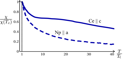
Figure 1: Local moments are seen in the Curie-Weiss susceptibilities: CeCoIn₅($T_{c}=2.3K$)shishido02 and NpPd₅Al₂($T_{c}=4.9K)$aoki08 are reproduced and rescaled by $\chi(T_{c})$ to show their similarity (data below $T_{c}$ not shown).

These observations motivate us to develop a theory of composite pairing incorporating valence fluctuations. Thus far, composite pairing has been studied within a two-channel Kondo modelcatk ; flint08 , treating only the local spin degrees of freedom. In this paper, we study composite pairing within a two-channel Anderson model, which permits us to include the charge degrees of freedom and model the effects of valence fluctuations on the superconductivity in the 5$f$ 115 materials. We predict a sharp shift in both the $f$-electron valence and quadrupole moment at the superconducting transition temperature. The quadrupole moment shift should manifest as a shift either in the nuclear quadrupole resonance (NQR) frequency, for Ce$M$In₅ or the Mössbauer quadrupole splitting, for NpPd₅Al₂, and we make concrete predictions for these shifts in Section  V.

The two-channel Anderson model is the natural extension of the two-channel Kondo model.

$$H=H_{c}+\sum_{j}H_{a}(j)+\sum_{j}H_{V}(j).$$ (2)

Here the local atomic Hamiltonian at site $j$ is,

$$H_{a}(j)=E_{0}X_{00}(j)+E_{2}X_{22}(j)+\sum_{\sigma}\epsilon_{f}X_{\sigma\sigma}(j),$$ (3)

where the $X$’s are the Hubbard operatorshubbard64 : $X_{00}=|0\rangle\langle 0|$, $X_{22}=|2\rangle\langle 2|$, and $X_{\sigma\sigma}=|\sigma\rangle\langle\sigma|$. The atomic states $|0\rangle$, $|\sigma\rangle$ and $|2\rangle$ are shown in Figure 2, where we take the doubly occupied state to be a singlet containing $f$-electrons in two orthogonal channels,

$$|2\rangle\equiv|\Gamma_{2}\otimes\Gamma_{1}\rangle_{s}=\frac{1}{\sqrt{2}}\sum_{\sigma=\pm 1}{\rm sgn}(\sigma)f^{\dagger}_{\Gamma_{2}\sigma}f^{\dagger}_{\Gamma_{1}\ -\sigma}|0\rangle.$$ (4)

The orthogonality of these two channels is essential to the superconductivity, and we take the Coulomb energy for two electrons in the same channel to be infinite, making this model closer to two copies of the infinite-$U$ Anderson model than to the finite-$U$ modelbolech . These $f$-electrons hybridize with a bath of conduction electrons, $H_{c}=\sum_{{\bf{k}},\sigma}\epsilon_{\bf{k}}c^{\dagger}_{{\bf{k}}\sigma}c_{{\bf{k}}\sigma}$ in two different channels

$$H_{V}(j)=\sum_{j}V_{1}\psi^{\dagger}_{1j\sigma}X_{0\sigma}(j)+\mathrm{h.c.}+V_{2}\psi^{\dagger}_{2j\sigma}\tilde{\sigma}X_{-\sigma 2}(j)+\mathrm{h.c.},$$ (5)

where the $\psi_{\Gamma j\sigma}$ are Wannier states representing a conduction electron in symmetry $\Gamma$ on site $j$. $X_{0\sigma}=|0\rangle\langle\sigma|$ and $X_{2\sigma}=|2\rangle\langle\sigma|$ are the Hubbard operators between the singly occupied state and empty or doubly occupied states, respectively (see Fig. 3). Here we have adopted the notation of Ce atoms, whose ground state is a $4f^{1}$ doublet, but this formalism also applies to Np $5f^{3}$ atoms, where both $|0\rangle\equiv|5f^{4}\rangle$ and $|2\rangle\equiv|5f^{2}\rangle$ are $J=4$ crystal field singlets, while $|\sigma\rangle$ represents one of the $J=9/2$ crystal field doublets of $5f^{3}$.

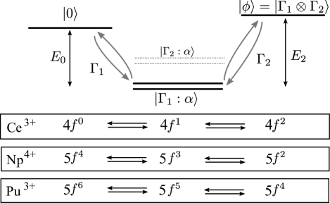
Figure 2: Virtual charge fluctuations of a two channel Anderson impurity, where the addition and removal of an $f$-electron occur in channels $\Gamma_{1}$ and $\Gamma_{2}$ of different crystal field symmetry. The ground state is a Kramer’s doublet, while the excited states $|0\rangle$, $|2\rangle$ are singlets. The excited doublet $|\Gamma_{2}:\alpha\rangle$ represents a higher lying crystal-field level and is excluded from the Hilbert space of the problem. The relevant charge states of Ce³⁺ (4$f^{1}$), Np⁴⁺ (5$f^{3}$) and Pu³⁺ (5$f^{5}$) are indicated.

To develop a controlled treatment of superconductivity in the two-channel Anderson model, we introduce a large-$N$ expansion. Preserving the time-reversal symmetries of spins is essential to capture singlet superconductivity in the entire family of large $N$ models, and large $N$ methods based on $SU(N)$ spins, like the usual slave boson approach, will lose time-reversal symmetry for any $N>2$. Treating superconductivity in the Kondo model therefore requires symplectic spins, the generators of the $SP(N)$ groupflint08 ,

$$S_{\alpha\beta}=f^{\dagger}_{\alpha}f_{\beta}-\tilde{\alpha}\tilde{\beta}f^{\dagger}_{-\beta}f_{-\alpha}.$$ (6)

Here $N$ is an even integer and the indices

$$\alpha\in\{\pm 1,\pm 2,\ldots\pm N/2\}$$ (7)

are integers running from $-N/2$ to $N/2$, excluding zero. We employ the notation $\tilde{\alpha}\equiv\mathrm{sgn}(\alpha)$. These spin operators invert under time-reversal $\mathbf{S}\to\theta\mathbf{S}\theta^{-1}=-\mathbf{S}$ and generate rotations that commute with the time-reversal operatorflint08 .

Physically, the spin fluctuations of a local moment are generated by valence fluctuations. Theoretically, these valence fluctuations can be described by Hubbard operators, and in a symplectic-$N$ generalization of the Anderson model, anticommuting two such Hubbard operators must generate a symplectic spin, satisfying the relations:

$$\left\{X_{0\alpha},X_{\beta 0}\right\} = X_{\alpha\beta}+X_{00}\delta_{\alpha\beta}$$

$$= S_{\alpha\beta}+\left(X_{00}+\frac{X_{\gamma\gamma}}{N}\right)\delta_{\alpha,\beta},$$

where the last equality follows from the traceless definition of the symplectic spin operator, $S_{\alpha\beta}=X_{\alpha\beta}-\frac{X_{\gamma\gamma}}{N}\delta_{\alpha\beta}$. In Section II, we show that a proper symplectic representation requires the introduction of two slave bosons to treat the Hubbard operators in a single channel:

$$X_{0\alpha} = b^{\dagger}f_{\alpha}+a^{\dagger}\tilde{\alpha}f_{-\alpha}^{\dagger}$$ (9)

$$X_{00} = b^{\dagger}b+a^{\dagger}a.$$ (10)

As we shall demonstrate, these symplectic Hubbard operators maintain the invariance of the Anderson Hamiltonian with respect to the $SU(2)$ particle-hole transformation, $f_{\sigma}\to\cos\theta\,f_{\sigma}+\mathrm{sign}(\sigma)\sin\theta\,f^{\dagger}_{-\sigma}$affleck88 . This extension of the slave boson representation with local $SU(2)$ gauge symmetry was originally introduced by Wen and Lee as a mean-field treatment of the $t-J$ modelwenlee96 . Here we show that these Hubbard operators maintain the $SU(2)$ gauge symmetry for arbitrary $SP(N)$ versions of the infinite $U$ Anderson and $t-J$ models. This $SU(2)$ gauge symmetry is essential for eliminating the false appearance of s-wave superconductivity in the finite-$U$ Anderson model, where the two channels are identical.

What do we learn from this Anderson model picture of composite pairing? A key result is that the amount of composite pairing can be written in a simple gauge-invariant form as

$$\Delta_{\text{SC}}=\langle X_{02}\rangle\propto\langle\psi^{\dagger}_{1}\vec{\sigma}\left(i\sigma_{2}\right)\psi^{\dagger}_{2}\cdot\vec{S}_{f}\rangle,$$ (11)

where the Hubbard operator $X_{02}=|0\rangle\langle 2|$ mixes the empty and doubly occupied states. This mixing resembles an intra-atomic version of the negative-$U$ pairing state, but double occupancy costs a large, positive energy. The physical consequence of this mixing is a redistribution of the charge in the $f$-electron orbitals, as the three charge states: empty, singly and doubly occupied, all have different charge distributions. Such a rearrangement not only changes the total charge in the $f$-shell, a monopole effect, but also will result in a quadrupole moment associated with the superconductivity. This quadrupole moment will lead to modified electric field gradients that should be detectable as a sharp shift in the nuclear quadrupolar resonance (NQR) frequency at the neighboring nuclei, or as a sharp shift in the Mössbauer quadrupolar splitting at the $f$-electron nuclei.

This paper is organized as follows. First we introduce the symplectic Hubbard operators in section II and demonstrate that the symplectic-$N$ and $SU(N)$ large-$N$ limits are identical for a single channel. We then generalize this formalism to the case of two channels in Section III and show how composite pairing naturally appears as a mixing of the empty and doubly occupied states. The mean-field solution is presented in Section IV, in which we demonstrate how the superconducting transition temperature increases with increasing mixed valence. In Section V, we calculate the charge distribution of the $f$-orbitals in the state with composite pairing and make a concrete prediction for a shift in the NQR frequency at $T_{c}$ in CeCoIn₅. Finally, section VI discusses the implications for the finite-$U$ Anderson model and examines the broader implications of our results.

II Symplectic Hubbard operators

Composite pairing was originally discussed in the two channel Kondo modelcatk , where it is found in the symplectic-$N$ limitflint08 , which maintains the time-inversion properties of spins in the large $N$ limit by using symplectic spins. Correctly including time-reversal symmetry allows the formation of Cooper pairs, and thus superconductivity. In order to treat composite pairing within a large $N$ Anderson model treatment, we would like to develop a set of Hubbard operators that maintain this time-reversal property in the large $N$ limit. Hubbard operators, like $X_{ab}=|a\rangle\langle b|$, are projectors between the local states, $|0,\sigma\rangle$ of the infinite $U$ Anderson model, describing both charge, $X_{0\sigma}$ and spin, $X_{\sigma\sigma^{\prime}}$ fluctuations.

Starting from a spin state $|\sigma\rangle$, hopping an electron off and back onto the site generates a spin flip: this condition defines the Hubbard operators within a single channel, where the Hubbard operators must satisfy a graded Lie algebra in which the projected hopping operators anti-commute, satisfying the algebra

$$\left\{X_{\alpha 0},X_{0\beta}\right\}=X_{\alpha\beta}+X_{00}\delta_{\alpha\beta}$$ (12)

Now the traceless part of $X_{\alpha\beta}$ defines a spin operator,

$$S_{\alpha\beta}=X_{\alpha\beta}-\frac{\delta_{\alpha\beta}}{N}X_{\gamma\gamma}$$

so that quite generally, Hubbard operators must satisfy an algebra of the form

$$\left\{X_{\alpha 0},X_{0\beta}\right\}=S_{\alpha\beta}+\left(X_{00}+\frac{X_{\gamma\gamma}}{N}\right)\delta_{\alpha\beta}$$ (13)

Thus the commutation algebra of the Hubbard operators generates the spin operators of the local moments. In the traditional slave boson approachcoleman83 , the Hubbard operators are written $X_{0\alpha}=b^{\dagger}f_{\alpha}$. The spin operators generated by this procedure are the generators of $SU(N)$, since

$$\{f^{\dagger}_{\alpha}b,b^{\dagger}f_{\beta}\}=\overbrace{(f^{\dagger}_{\alpha}f_{\beta}-\frac{n_{f}}{N}\delta_{\alpha\beta})}^{S^{SU(N)}_{\alpha\beta}}+\left(b^{\dagger}b+\frac{n_{f}}{N}\right)\delta_{\alpha\beta}$$ (14)

where $S^{SU(N)}_{\alpha\beta}$ is the well-known form of $SU(N)$ spins. It is thus no wonder that this approach cannot treat superconductivity in the large $N$ limit, for there are no spin singlet Cooper pairs for $SU(N)$ with $N>2$. We require instead that the spin fluctuations generated by Hubbard operators are symplectic spin operators

$$S_{\alpha\beta}=f^{\dagger}_{\alpha}f_{\beta}-{\rm sgn}(\alpha\beta)f^{\dagger}_{-\beta}f_{-\alpha}$$ (15)

We now show that the Hubbard algebra(I) can be satisfied with symplectic spins, using the introduction of two slave bosons,

$$X_{\alpha 0} = f^{\dagger}_{\alpha}b+\tilde{\alpha}f_{-\alpha}a,$$ (16)

$$X_{0\beta} = b^{\dagger}f_{\beta}+a^{\dagger}\tilde{\beta}f_{-\beta}^{\dagger}.$$ (17)

These operators satisfy the Hubbard operator algebra (12), but now

$$X_{\alpha\beta}=f^{\dagger}_{\alpha}f_{\beta}+{\tilde{\alpha}\tilde{\beta}}f_{-\alpha}f^{\dagger}_{-\beta}=S_{\alpha\beta}+\delta_{\alpha\beta}$$ (18)

describes a symplectic spin operator while

$$X_{00}=b^{\dagger}b+a^{\dagger}a$$ (19)

is the representation of the empty state operator.

At first sight, the expedience of this new representation might be questioned: why exchange the simplicity of the original Hubbard operators, $X_{ab}=|a\rangle\langle b|$ for a profusion of slave boson fields? However, while the original Hubbard operators may appear to be simple, they are singularly awkward to treat in many-body theory keiter71 , due to their noncanonical anti-commutation algebra, (I). The slave boson representation allows us to represent these operators in terms of canonical bosons and fermions. By doubling the number of slave bosons the symplectic character of the spins is preserved at all even values of $N$, and we shall see that this process encodes the hard-to-enforce Gutzwiller projection as a mathematically tractable $SU(2)$ gauge symmetry.

Physical spins are neutral, and thus possess a continuous particle-hole symmetry. This property is maintained by symplectic spin operators, which can be seen most naturally by introducing the generalized pair creation operators,

$$\Psi^{\dagger}=\frac{1}{2}\sum_{\alpha}\tilde{\alpha}f^{\dagger}_{\alpha}f^{\dagger}_{-\alpha}=\sum_{\alpha>0}f^{\dagger}_{\alpha}f^{\dagger}_{-\alpha},$$ (20)

which allow us to construct the isospin vector, $\vec{\Psi}=(\Psi_{1},\Psi_{2},\Psi_{3})$, where

$$\Psi_{1} = \left(\Psi^{\dagger}+\Psi\right),\;\;\Psi_{2}=-i\left(\Psi^{\dagger}-\Psi\right)$$ (21)

$$\Psi_{3} = \sum_{\alpha>0}(f^{\dagger}_{\alpha}f_{\alpha}-f_{-\alpha}f^{\dagger}_{-\alpha})=n_{s}-N/2,$$ (22)

and $n_{s}\equiv\sum_{\alpha}\langle\alpha|f^{\dagger}_{\alpha}f_{\alpha}|\alpha\rangle$ is the fermion number in the singly-occupied states, i.e. $n_{s}$ plays the role of the number of spins in the above constraint $\Psi_{3}$. The isospin vector commutes with symplectic spins, $\left[\vec{\Psi},S_{\alpha\beta}\right]=0$, showing that the symplectic spins possess an $SU(2)$ gauge symmetry: a continuous particle-hole symmetry that allows us to redefine the spinon, $f_{\alpha}\rightarrow uf_{\alpha}+v\tilde{\alpha}f^{\dagger}_{-\alpha}$. This symmetry is reflected in the requirement of two types of bosons, as the empty state does not distinguish between zero and two fermions, and thus requires two bosons to keep track of the two ways of representing the empty state, $b^{\dagger}|\Omega\rangle$ and $a^{\dagger}f^{\dagger}_{\uparrow}f^{\dagger}_{\downarrow}|\Omega\rangle=a^{\dagger}\Psi^{\dagger}|\Omega\rangle$, where $|\Omega\rangle$ is the slave-boson vacuum. Of course, there is only one physical empty state, as becomes clear when we restrict these Hubbard operators to the physical subspace. In order to faithfully represent the symplectic spins, the sum of the spin and charge fluctuations must be fixed, $\vec{S}^{2}+\vec{\Psi}^{2}=\frac{N}{2}(\frac{N}{2}+2)$[flint08, ]. While this constraint is enforced by setting $\vec{\Psi}=0$ in the pure spin model, here we must equate our two types of charge fluctuations, by setting

$$Q_{3} = \sum_{\alpha}f^{\dagger}_{\alpha}f_{\alpha}-N/2+b^{\dagger}b-a^{\dagger}a=0$$ (23)

$$Q_{+} = \sum_{\alpha>0}f_{\alpha}^{\dagger}f_{-\alpha}^{\dagger}+b^{\dagger}a=0$$ (24)

$$Q_{-} = \sum_{\alpha>0}f_{-\alpha}f_{\alpha}+a^{\dagger}b=0.$$ (25)

The three operators $(Q_{\pm},Q_{3})$ commute with the Hamiltonian, which imposes the constraints associated with the physical Hilbert space. The constraint reflects the neutrality of the spins under charge conjugation: $Q_{3}$ conserves total electromagnetic charge, and prevents double occupancy, while $Q_{\pm}$ kills any states with s-wave pairs on-site. From the form of $Q_{3}$, we see that $b$ and $a$ have opposite gauge charges. The gauge invariant states satisfying the constraint (for $N=2$) are,

$$|\alpha\rangle = f^{\dagger}_{\alpha}|\Omega\rangle$$ (26)

$$|0\rangle = \left(b^{\dagger}+a^{\dagger}\Psi^{\dagger}\right)|\Omega\rangle.$$ (27)

The symplectic Hubbard operators can be written more compactly by using Nambu notation,

$$X_{0\alpha}=B^{\dagger}\tilde{f}_{\alpha},\;X_{00}=B^{\dagger}B$$ (28)

where

$$B=\left(\!\begin{array}[]{c}b\cr a\end{array}\!\right),\;\tilde{f}_{\alpha}=\left(\!\begin{array}[]{c}f_{\alpha}\\ \tilde{\alpha}f_{-\alpha}^{\dagger}\end{array}\!\right),$$ (33)

The constraint becomes $\vec{Q}=B^{\dagger}\vec{\tau}B+\sum_{\alpha>0}\tilde{f}_{\alpha}^{\dagger}\vec{\tau}\tilde{f}_{\alpha}=0$. For $N=2$, these Hubbard operators are the $SU(2)$ slave bosons introduced by Wen and Lee in the context of the $t-J$ modelwenlee96 . Here, it becomes clear that the $SU(2)$ structure is a consequence of symplectic symmetry, present in both the symplectic-$N$ Kondo and Anderson models, not just for $N=2$, but for all $N$. This symmetry can be physically interpreted as the result of valence fluctuations in the presence of a particle-hole symmetric spin.

The Hamiltonian of the one channel, single impurity infinite-$U$ Anderson model can now be expressed via symplectic slave bosons as follows:

$$H = \sum_{{\bf{k}},\alpha}\epsilon_{\bf{k}}c^{\dagger}_{{\bf{k}}\alpha}c_{{\bf{k}}\alpha}+E_{0}(b^{\dagger}b+a^{\dagger}a)$$ (34)

$$+ \sum_{\alpha}V\psi^{\dagger}_{\alpha}(b^{\dagger}f_{\alpha}+a^{\dagger}\tilde{\alpha}f_{-\alpha}^{\dagger})+\mathrm{h.c.}$$ (35)

The $SU$(2) gauge symmetry of this model becomes particularly evident in the field-theoretical formulation, where the partition function is written as a path integral:

$$Z=\int\mathcal{D}[\tilde{\psi}^{\dagger},\tilde{\psi},\tilde{f}^{\dagger},\tilde{f},B^{\dagger},B]e^{-S},$$ (36)

where the Euclidean action $S$ is written in Nambu notation as follows

$$S=\!\int\limits_{0}^{\beta}\!\mathrm{d}\tau\!\sum_{\mathbf{k},{\alpha>0}}\tilde{\psi}_{\mathbf{k}{\alpha}}^{\dagger}(\partial_{\tau}+\epsilon_{k}\tau_{3})\tilde{\psi}_{\mathbf{k}{\alpha}}+\!\sum_{j}\!\left\{\frac{1}{2}{\hbox{Tr}}\left[\tau_{3}\mathcal{A}^{\dagger}_{j}(\partial_{\tau}\!+E_{0}\!+\vec{\lambda}_{j}\cdot\vec{\tau})\mathcal{A}_{j}\right]+\sum_{\alpha>0}\left[\tilde{f}^{\dagger}_{j{\alpha}}(\partial_{\tau}+\vec{\lambda}_{j}\cdot\vec{\tau})\tilde{f}_{j{\alpha}}+\left(V\tilde{\psi}^{\dagger}_{j\alpha}\mathcal{A}_{j}^{\dagger}\tilde{f}_{j\alpha}+\text{h.c.}\right)\right]\!\right\}\!,$$ (27)

where $\tilde{\psi}^{\dagger}_{\alpha}=(\psi^{\dagger}_{\alpha},\tilde{\alpha}\psi_{-\alpha})$, $\beta=1/T$ is the inverse temperature and the $SU$(2) matrix $\mathcal{A}_{j}$ of slave bosons is defined as

$$\mathcal{A}_{j}=\left[\!\begin{matrix}b_{j}&a_{j}^{\dagger}\cr a_{j}&-b_{j}^{\dagger}\end{matrix}\!\right].$$ (39)

The first three terms in Eq. (27) describe the dynamics of conduction electrons $\tilde{\psi}$, $f$-electrons $\tilde{f}$ and the slave bosons $B$ respectively, with the constraint $\vec{Q}=0$ imposed by introducing the vector of Lagrange multipliers $\vec{\lambda}$. The last term describes the coupling between the f-atom and conduction electrons.

The action (27) is manifestly invariant under the $SU(2)$ gauge transformation via unitary matrix $\hat{g}_{j}$:

$$\tilde{f}_{j}\rightarrow\hat{g}_{j}\tilde{f}_{j}, \quad\tilde{\psi}_{j}\rightarrow\hat{g}_{j}\tilde{\psi}_{j},\quad\mathcal{A}_{j}\rightarrow\hat{g}_{j}\mathcal{A}_{j}$$

$$\vec{\lambda_{j}}\cdot\vec{\tau}\rightarrow\vec{\lambda_{j}}\cdot\vec{\tau}-\hat{g}_{j}^{\dagger}\partial_{\tau}\hat{g}_{j}$$

At first sight, the $a$ hybridization term in the Hamiltonian, (35) appears to give rise to $\langle c^{\dagger}f^{\dagger}\rangle$ pairing terms, however, the $SU(2)$ symmetry allows to redefine the fields, making the substitution

$$B=\binom{b}{a}\rightarrow\hat{g}B=\binom{b^{\prime}}{0}.$$ (41)

This transformation eliminates the composite $s$-wave pairing, $b^{\dagger}f_{\alpha}+a^{\dagger}f^{\dagger}_{-\alpha}\tilde{\alpha}\rightarrow b^{{}^{\prime}\dagger}f^{\prime}_{\alpha}$, recovering the usual $U(1)$ slave boson Hamiltonian.

One of the the most important physical consequences encoded in this local gauge symmetry is the complete suppression of any $s$-wave pairing in the single channel Anderson model. Indeed, the constraint operator $Q_{+}=\sum_{\alpha>0}f^{\dagger}_{\alpha}f^{\dagger}_{-\alpha}+b^{\dagger}a$ may be directly interpreted as the on-site $s$-wave pair creation operator plus a term $b^{\dagger}a$ that can be removed by the above gauge transformation. In particular, the mean-field constraint

$$\langle Q_{+}\rangle\equiv\langle\hbox{s-wave pair creation operator}\rangle=0$$

hard-wires the strong suppression of local $s$-wave pairing into the formalism. In the language of superconductivity, the constraint $Q_{\pm}=0$ plays the role of an infinite Coulomb pseudopotential, or renormalized electron-electron interaction, $\mu^{*}$. It is the satisfaction of this constraint that drives anisotropic composite pairing.

III The two channel Anderson lattice model

We turn now to the two channel lattice Anderson model, where the two channels involve charge fluctuations to the “empty” and “doubly” occupied states; here we use the language of Ce³⁺ whose ground state configuration is $f^{1}$, but this model captures any system with valence fluctuations from $f^{n-1}\rightleftharpoons f^{n}\rightleftharpoons f^{n+1}$, where $n$ is odd. For $n=1$, the empty state, $|0\rangle$ is trivially a singlet, and we choose the doubly occupied state to be a singlet formed from electrons in two orthogonal channels,

$$|2\rangle=\tilde{\alpha}f^{\dagger}_{\Gamma_{1},\alpha}f^{\dagger}_{\Gamma_{2},-\alpha}|0\rangle,$$ (42)

where $|\Gamma_{1}:\pm\rangle\equiv|\pm\rangle$ is the ground state crystal field doublet, and $|\Gamma_{2}:\pm\rangle$ is an excited crystal field doublet. In the finite-$U$ Anderson model, the symmetries of the electron addition and removal processes are identical, but here Hund’s rules force the second electron to be placed in a channel orthogonal to the first.

The local atomic Hamiltonian at site $j$ can be expressed in terms of Hubbard operators,

$$H_{a}(j) = E_{0}X_{00}(j)+E_{2}X_{22}(j)+\sum_{\sigma}\epsilon_{f}X_{\sigma\sigma}(j)$$ (43)

$$+ \sum_{\sigma}\Delta_{CF}X_{\Gamma_{2}\sigma;\Gamma_{2}\sigma},$$ (44)

where the $X$’s are the Hubbard operators projecting into the empty, $X_{00}=|0\rangle\langle 0|$ and doubly occupied, $X_{22}=|2\rangle\langle 2|$ states, as well as the projectors into the ground state, $X_{\sigma\sigma}=|\Gamma_{1}\sigma\rangle\langle\Gamma_{1}\sigma|\equiv|\sigma\rangle\langle\sigma|$, and excited, $X_{\Gamma_{2}\sigma;\Gamma_{2}\sigma}=|\Gamma_{2}\sigma\rangle\langle\Gamma_{2}\sigma|$ crystal field doublets. If we measure the energies from the $f$-electron level, $E_{0}=-\epsilon_{f}$ and $E_{2}=U_{12}+\epsilon_{f}$ are both positive, where $U_{12}$ is the Hubbard $U$ for the doubly occupied state with one electron in $\Gamma_{1}$ and the other in $\Gamma_{2}$. We take $U_{11},U_{22}\rightarrow\infty$. The $f$-electrons hybridize with a bath of conduction electrons, $H_{c}=\sum_{{\bf{k}},\sigma}\epsilon_{\bf{k}}c^{\dagger}_{{\bf{k}}\sigma}c_{{\bf{k}}\sigma}$ in two different channels,

$$H_{V}(j)\!=\!\sum_{j}V_{1}\psi^{\dagger}_{1j\sigma}X_{0\sigma}(j)+V_{2}\tilde{\sigma}\psi^{\dagger}_{2j\sigma}X_{-\sigma 2}(j)+\text{h.c.}$$ (45)

The angular momentum dependence is hidden inside the conduction Wannier states,

$$\psi_{\Gamma j\sigma}=\sum_{{\bf{k}}}{\mathrm{e}}^{-i{\bf{k}}\cdot{\bf{R}}_{j}}\left[\Phi_{\Gamma{\bf{k}}}\right]_{\sigma\sigma^{\prime}}c_{{\bf{k}}\sigma^{\prime}},\qquad(\Gamma=1,2)$$ (46)

where the crystal field form-factors $\left[\Phi_{\Gamma{\bf{k}}}\right]_{\sigma\sigma^{\prime}}=\langle k\Gamma\sigma^{\prime}|{\bf{k}}\sigma\rangle$ are proportional to unitary matrices. $X_{0\sigma}=|0\rangle\langle\Gamma_{1}\sigma|$ and $X_{2\sigma}=|2\rangle\langle\Gamma_{1}\sigma|$ are the Hubbard operators between the singly occupied ground state and empty or doubly occupied states, respectively.

The symplectic-$N$ Hubbard operators describing charge fluctuations in the two channels are a simple generalization of those used for a single channel. For a single site, these are given by

$$X_{0\alpha}=b_{0}^{\dagger}f_{\alpha}+a_{0}^{\dagger}\tilde{\alpha}f_{-\alpha}^{\dagger},\;X_{00}=b_{0}^{\dagger}b_{0}+a_{0}^{\dagger}a_{0},$$ (47)

$$X_{2\alpha}=b_{2}^{\dagger}f_{\alpha}-a_{2}^{\dagger}\tilde{\alpha}f_{-\alpha}^{\dagger},\;X_{22}=b_{2}^{\dagger}b_{2}+a_{2}^{\dagger}a_{2},$$ (48)

which can again be written more compactly by using a Nambu notation,

$$X_{0\alpha} = B_{0}^{\dagger}\tilde{f}_{\alpha},\qquad X_{2\alpha}=B_{2}^{\dagger}\tilde{f}_{\alpha}$$ (49)

$$X_{00} = B_{0}^{\dagger}B_{0},\qquad X_{22}=B_{2}^{\dagger}B_{2},$$ (50)

where

$$B_{0}=\left(\begin{array}[]{c}b_{0}\cr a_{0}\end{array}\right),\qquad B_{2}=\left(\begin{array}[]{c}b_{2}\cr-a_{2}\end{array}\right).$$ (51)

We are free to choose the sign of $a_{2}$, and in the above we have chosen the negative sign to preserve continuity with the results from the two channel Kondo modelflint08 . The doubly occupied state is then,

$$|2\rangle=\left(b_{2}^{\dagger}-a_{2}^{\dagger}\Psi^{\dagger}\right)|\Omega\rangle,$$ (52)

where $\Psi^{\dagger}=\sum_{\alpha>0}f^{\dagger}_{\alpha}f^{\dagger}_{-\alpha}$ is the pair creation operator, as before.

Figure 3: The six physical states in the Hilbert space of the $N=2$ two channel Anderson model, representing the ground state and excited crystal field doublets, and the empty and doubly occupied singlets. Arrows show the operators that move between states in the Hilbert space.

In the two channel model case the constraint becomes,

$$\vec{Q}=B^{\dagger}_{0}\vec{\tau}B_{0}+B^{\dagger}_{2}\vec{\tau}B_{2}+\tilde{f}_{\alpha}^{\dagger}\vec{\tau}\tilde{f}_{\alpha}=0.$$ (53)

The intersection of the two Hubbard algebras gives rise to an extra doublet,

$$|\Gamma_{2}\alpha\rangle=\left(b^{\dagger}_{0}a_{2}^{\dagger}+b^{\dagger}_{2}a_{0}^{\dagger}\right)f^{\dagger}_{\alpha}|\Omega\rangle,$$ (54)

which we interpret as the excited crystal field doublet because it is reached by destroying a $\Gamma_{1}$ electron from the doubly occupied state, leaving behind the $\Gamma_{2}$ electron. However, this extra doublet is not killed by $X_{00}$ or $X_{22}$, which are no longer the projectors within this larger space. The full Hamiltonian term for this state must therefore be quartic in the bosons, and subtract off the contribution from $X_{00}$, $X_{22}$ and $X_{\sigma\sigma}$,

$$\left[\Delta_{\text{CF}}\!-\!(E_{0}\!+E_{2}\!+\epsilon_{f})\right]\!\left(\!b_{0}^{\dagger}a_{2}^{\dagger}+a_{0}^{\dagger}b_{2}^{\dagger}\right)\!\left(b_{0}a_{2}\!+a_{0}b_{2}\right),$$ (55)

where $\Delta_{\text{CF}}$ is the crystal field effect splitting. We neglect this term for much of our analysis, as it turns out to be irrelevant for the superconducting states of interest.

In addition to an extra state, there are two additional operators,

$$X_{20} = \{X_{2\alpha},X_{\alpha 0}\}=B_{2}^{\dagger}B_{0}=b^{\dagger}_{2}b_{0}-a^{\dagger}_{2}a_{0}$$ (56)

$$X_{\Gamma_{1}\alpha;\Gamma_{2}\beta} = -\{X_{0\alpha},X_{2\beta}\}=B_{0}^{\dagger}(-i\tau_{2})\left[B_{2}^{\dagger}\right]^{T}\hskip-8.53581pt\tilde{\alpha}\delta_{\alpha,-\beta}$$ (57)

$$= \left(b^{\dagger}_{0}a^{\dagger}_{2}-b^{\dagger}_{2}a^{\dagger}_{0}\right)\tilde{\alpha}\delta_{\alpha,-\beta}.$$ (58)

The operator $X_{\Gamma_{1}\alpha;\Gamma_{2}\beta}$ mixes the ground state and excited crystal field doublets, leading to a composite density wave state, $\langle c^{\dagger}_{1}ff^{\dagger}c_{2}\rangle$. As this state mixes two irreducible representations of the point group, it necessarily breaks the crystal symmetry and this phase can also be called a composite nematic. This mixing resembles the ordered state proposed for URu₂Si₂[haule09, ], which mixes ground state and excited singlets.

The operator $X_{20}=|2\rangle\langle 0|$ mixes the empty and doubly occupied states, and can be thought of as a pair creation operator. As we show in the next section, this operator acquires an expectation value when composite pairing develops. The development of an intra-atomic order parameter $\langle X_{02}\rangle$ is reminiscent of pairing in a negative (attractive)-$U$ atomanderson75 , but unlike a negative-$U$ atom, the empty and doubly occupied sites are excited states of the atomic Hamiltonian, and they are only partially occupied as a result of valence fluctuations. Furthermore, the paired state is an anisotropic singlet with nodes. In the case of the Ce 115 materials, this product has $d$-wave symmetry flint08 .

Again, we should consider the question of supressing s-wave superconductivity. Here,

$$Q_{+}=\sum_{\alpha>0}f^{\dagger}_{\alpha}f^{\dagger}_{-\alpha}+b^{\dagger}_{0}a_{0}+b^{\dagger}_{2}a_{2}.$$

We know from the one channel model that $a_{0}$ can be removed by a gauge transformation, eliminating the middle term, but the $b^{\dagger}_{2}a_{2}$ term cannot be uniformly eliminated. However, it will only be nonzero in a state where both $\langle X_{20}\rangle$ and $\langle X_{\Gamma_{1}\alpha;\Gamma_{2}\beta}\rangle$ are nonzero, implying coexisting superconducting and composite nematic order. Under normal circumstances, these two phases repel one another, and s-wave superconductivity is wholly suppressed.

IV The large $N$ two channel Anderson lattice model

We are now able to write the symplectic-$N$ two channel Anderson lattice model in terms of the symplectic Hubbard operators,

$$H = \sum_{\bf{k}}\epsilon_{k}c^{\dagger}_{{\bf{k}}\alpha}c_{{\bf{k}}\alpha}+\sum_{j}E_{0}B_{0}^{\dagger}(j)B_{0}(j)+E_{2}B_{2}^{\dagger}(j)B_{2}(j)$$ (61)

$$+\frac{V_{1}}{\sqrt{N/2}}\sum_{j}\psi^{\dagger}_{1j\alpha}B_{0}^{\dagger}(j)\tilde{f}_{j\alpha}+\mathrm{h.c.}$$

$$+\frac{V_{2}}{\sqrt{N/2}}\sum_{j}\psi^{\dagger}_{2j\alpha}\tilde{\alpha}\tilde{f}_{j-\alpha}^{\dagger}B_{2}(j)+\mathrm{h.c.}$$

In order to keep the Hamiltonian extensive in $N$, we have rescaled the hybridization terms by $(N/2)^{-1/2}$, so that they recover the correct $N=2$ form, (45). This rescaling implicitly assumes that the slave bosons fields $B_{l}\;(l=0,2)$ will acquire a magntitude of order $O(\sqrt{N})$. Since there are only two flavors of bosons, for the bosons to play a role in the large $N$ limit, they must condense.

Following the construction that led to the path integral description of the single-channel Anderson model (27) above, one can write down the Euclidean action that corresponds to this Hamiltonian:

$$S_{2}[\tilde{\psi},\tilde{f},\mathcal{A}_{0},\mathcal{A}_{2}] = \int\limits_{0}^{\beta}\mathrm{d}\tau\sum_{\mathbf{k},{\alpha>0}}\tilde{\psi}_{\mathbf{k}{\alpha}}^{\dagger}(\partial_{\tau}+\epsilon_{k}\tau_{3})\tilde{\psi}_{\mathbf{k}\alpha}$$ (64)

$$+\sum_{j}\left\{\frac{1}{2}{\hbox{Tr}}\left[\tau_{3}\mathcal{A}^{\dagger}_{0j}(\partial_{\tau}+E_{0}+\vec{\lambda}_{j}\cdot\vec{\tau})\mathcal{A}_{0j}\right]+\frac{1}{2}{\hbox{Tr}}\left[\tau_{3}\mathcal{A}^{\dagger}_{2j}(\partial_{\tau}+E_{2}+\vec{\lambda}_{j}\cdot\vec{\tau})\mathcal{A}_{2j}\right]\right\}$$

$$+\sum_{\alpha>0}\left\{\tilde{f}^{\dagger}_{j{\alpha}}(\partial_{\tau}+\vec{\lambda}_{j}\cdot\vec{\tau})\tilde{f}_{j{\alpha}}+\left(\frac{V_{1}}{\sqrt{N/2}}\tilde{\psi}^{\dagger}_{1j{\alpha}}\mathcal{A}_{0j}^{\dagger}\tilde{f}_{j{\alpha}}+\frac{V_{2}}{\sqrt{N/2}}\tilde{\psi}^{\dagger}_{2j{\alpha}}\mathcal{A}_{2j}^{\dagger}\tilde{f}_{j{\alpha}}+\text{h.c.}\right)\right\},$$

where $\tilde{\psi}^{\dagger}_{\Gamma j{\alpha}}=(\psi^{\dagger}_{\Gamma j{\alpha}},{\rm sgn}({{\alpha}})\psi_{\Gamma j-{\alpha}})$ are Nambu spinors for the Wannier states in each channel. Above, we have collected the slave bosons into the $SU(2)$ matrices,

$$\mathcal{A}^{\dagger}_{0}=\left[\!\begin{matrix}b_{0}^{\dagger}&a_{0}^{\dagger}\cr a_{0}&-b_{0}\end{matrix}\!\right],\quad\mathcal{A}^{\dagger}_{2}=\left[\!\begin{matrix}a_{2}&b_{2}\cr b_{2}^{\dagger}&-a_{2}^{\dagger}\end{matrix}\!\right].$$ (65)

The action (64) remains manifestly invariant under the $SU(2)$ gauge symmetry $B_{l}\rightarrow\hat{g}_{j}B_{l}$, where $\hat{g}_{j}$ is an $SU(2)$ matrix. The matrices $\mathcal{A}_{0},\mathcal{A}_{2}$ transform under this gauge symmetry as $\mathcal{A}_{l}\rightarrow\hat{g}_{j}\mathcal{A}_{l}$, leaving the product

$$\mathcal{A}^{\dagger}_{2}\mathcal{A}_{0}=\left[\!\begin{matrix}b_{0}a_{2}+b_{2}a_{0}&a_{0}^{\dagger}a_{2}-b_{0}^{\dagger}b_{2}\cr b_{2}^{\dagger}b_{0}-a_{2}^{\dagger}a_{0}&b_{2}^{\dagger}a_{0}^{\dagger}+a_{2}^{\dagger}b_{0}^{\dagger}\end{matrix}\!\right]$$ (66)

gauge invariant.

The off-diagonal components of the product $\mathcal{A}^{\dagger}_{2}\mathcal{A}_{0}$ have the physical meaning of composite pairing between conduction and $f$-electrons. Indeed, in the Kondo limit, $E_{0},E_{2}\gg\pi\rho V^{2}$, we can connect the two channel Anderson model results to those from the two channel Kondo modelflint08 . A Schrieffer-Wolff transformation maps $b_{0}\rightarrow V_{1}$, $a_{0}\rightarrow\Delta_{1}$, $b_{2}\rightarrow\Delta_{2}$ and $a_{2}\rightarrow V_{2}$, where $V_{\Gamma}$ and $\Delta_{\Gamma}$ are the particle-hole and particle-particle hybridizations, respectively. We can now identify the off-diagonal components of $\mathcal{A}^{\dagger}_{2}\mathcal{A}_{0}\propto V_{1}\Delta_{2}-V_{2}\Delta_{1}$ with composite pairing. More generally, the components of $\mathcal{A}^{\dagger}_{2}\mathcal{A}_{0}$ can be identified with the state mixing operators,

$$\mathcal{A}^{\dagger}_{2}\mathcal{A}_{0}=\left[\!\begin{matrix}X_{\Gamma_{1}\Gamma_{2}}&-X_{02}\cr X_{20}&X_{\Gamma_{2}\Gamma_{1}}\end{matrix}\!\right],$$ (67)

which confirms the identification of $\langle X_{02}\rangle$ with composite pairing, and implies that the composite pair state contains an admixture of the empty and doubly occupied states.

To write down a translationally invariant Hamiltonian, we assume that the expectation values of the slave bosons are uniform, which allows us to write down the Hamiltonian in momentum space. To simplify this step, we temporarily drop the spin-orbit dependence of the Wannier functions, treating the form factors as spin-diagonal, $\psi_{\Gamma j\alpha}=\sum_{\bf{k}}c_{{\bf{k}}\alpha}\phi_{\Gamma{\bf{k}}}{\mathrm{e}}^{-i{\bf{k}}\cdot{\bf{R}}_{j}}$. This allows us to absorb the momentum dependence of the form-factors into the hybridizations by defining $V_{\Gamma{\bf{k}}}\equiv\frac{V_{\Gamma}}{\sqrt{N/2}}\phi_{\Gamma{\bf{k}}}$. To obtain the $d$-wave symmetry which arises naturally from the spin-orbit form factors flint08 , now we must explicitly make $V_{1k}V_{2k}$ $d$-wave. The full spin-orbit dependence can be restored in a similar manner to the two channel Kondo model flint08 . The Hamiltonian is,

$$H\! = \!\!\sum_{{\bf{k}}\alpha}\!\!\left(\epsilon_{k}c^{\dagger}_{{\bf{k}}\alpha}c_{{\bf{k}}\alpha}\!+V_{1{\bf{k}}}c^{\dagger}_{{\bf{k}}\alpha}B_{0}^{\dagger}\tilde{f}_{{\bf{k}}\alpha}\!+V_{2{\bf{k}}}c^{\dagger}_{{\bf{k}}\alpha}\tilde{\alpha}\tilde{f}_{{\bf{k}}-\alpha}^{\dagger}B_{2}\!+\text{h.c.}\!\right)$$ (69)

$$+\mathcal{N}_{s}\left(E_{0}B_{0}^{\dagger}B_{0}+E_{2}B_{2}^{\dagger}B_{2}\right),$$

where $\mathcal{N}_{s}$ is the number of lattice sites. As before, the $SU(2)$ constraint is implemented with a vector of Lagrange multipliers, $\vec{\lambda}$,

$$\vec{\lambda}\cdot\left(\sum_{\bf{k}}\tilde{f}^{\dagger}_{{\bf{k}}\alpha}\vec{\tau}\tilde{f}^{\dagger}_{{\bf{k}}\alpha}+B_{0}^{\dagger}\vec{\tau}B_{0}+B_{2}^{\dagger}\vec{\tau}B_{2}\right),$$ (70)

where we have also assumed that $\vec{\lambda}$ is translationally invariant, enforcing the constraint on average. This approximation becomes exact in the large $N$ limit.

The Hamiltonian can be re-written in the compact form with Nambu spinors,

$$\!H\! = \!\sum_{{\bf{k}}\alpha}\!\left(\tilde{c}^{\dagger}_{{\bf{k}}\alpha}\;\tilde{f}^{\dagger}_{{\bf{k}}\alpha}\right)\!\!\left[\!\begin{matrix}\epsilon_{\bf{k}}\tau_{3}&V_{1{\bf{k}}}\mathcal{A}_{0}^{\dagger}\!+V_{2{\bf{k}}}\mathcal{A}_{2}^{\dagger}\cr V_{1{\bf{k}}}\mathcal{A}_{0}\!+V_{2{\bf{k}}}\mathcal{A}_{2}\!&\vec{\lambda}\cdot\vec{\tau}\end{matrix}\!\right]\!\!\left(\!\!\begin{array}[]{c}\tilde{c}_{{\bf{k}}\alpha}\cr\tilde{f}_{{\bf{k}}\alpha}\end{array}\!\!\right)$$ (73)

$$+ \left[E_{0}B^{\dagger}_{0}B_{0}+E_{2}B^{\dagger}_{2}B_{2}+\vec{\lambda}\cdot\left(B^{\dagger}_{0}\vec{\tau}B_{0}+B^{\dagger}_{2}\vec{\tau}B_{2}\right)\right],$$ (74)

We note that while in the one-channel infinite-$U$ Anderson model (27), the spurious superconducting $s$-wave state was eliminated by fixing the $SU(2)$ gauge transformation, the two-channel model (64) generally possesses a composite superconducting ground state, which cannot be eliminated by a gauge fixing procedure. However we can always define a transformation $\hat{g}$ such that $a_{0}$ vanishes, so that $B_{0}^{\dagger}\rightarrow(b_{0}^{{}^{\prime}\dagger},0)$. In this new basis, the composite pairing operator $X_{02}=B_{0}^{\dagger}B_{2}$ (58) takes on the simple form, $X_{02}=b_{0}^{{}^{\prime}\dagger}b^{\prime}_{2}$.

IV.1 The mean field solution

In order to study the effects of mixed valence on the superconductivity, we examine the mean field solution of the composite pair state in the symplectic-$N$ limit. The bosons are replaced by their expectation values, $B_{l}\rightarrow\langle B_{l}\rangle\sim O(\sqrt{(}N))$, and the Hamiltonian (73) becomes quadratic in the fermions, which may be integrated out exactly, leading to the effective action $S_{eff}[B_{0},B_{2}]$ in terms of the boson fields only. The mean-field solution is then obtained as a saddle-point of this action:

$$\frac{\delta S_{eff}[B_{0},B_{2}]}{\delta{B_{l}}}=0.$$ (75)

We use the $SU(2)$ gauge symmetry to eliminate the $a_{0}$ boson, and now the composite pair state is defined by the nonzero expectation value of $\langle X_{02}\rangle=\langle b_{0}^{\dagger}b_{2}\rangle$. While the $a_{2}$ boson can in principle acquire an expectation value, it would lead to a uniform composite density wave solution, which is generally unstable to the composite pair solution. Therefore in what follows, we shall set $\langle a_{2}\rangle=0$. The resulting free energy can be rewritten in terms of our mean field parameters, where we replace $\langle b_{l}\rangle/\sqrt{N/2}$ with $b_{l}$ for clarity, (however keep in mind that these have lost their dynamics),

$$F = -NT\sum_{{\bf{k}}\pm}\log 2\cosh\frac{\beta\omega_{k\pm}}{2}$$ (77)

$$+\frac{N\mathcal{N}_{s}}{2}\left[b_{0}^{2}(E_{0}+\lambda_{3})+b_{2}^{2}(E_{2}+\lambda_{3})\right].$$

$\mathcal{N}_{s}$ is the number of sites, and the dispersion of the heavy electrons is given by four branches: $\omega_{k\pm}$ and $-\omega_{k\pm}$, where $\omega_{k\pm}=\sqrt{\alpha_{k}\pm\Gamma_{k}}$, and

$$\alpha_{k} = b_{+}^{2}+\frac{1}{2}(\epsilon_{{\bf{k}}}^{2}+\lambda_{3}^{2}+\lambda_{1}^{2}),\;\Gamma_{\bf{k}}=\sqrt{\alpha_{k}^{2}-\gamma_{k}^{2}}$$ (78)

$$\gamma_{k}^{2} = \left[\epsilon_{\bf{k}}\lambda_{3}-b_{-}^{2}\right]^{2}+\left[2V_{1{\bf{k}}}b_{0}V_{2{\bf{k}}}b_{2}-\epsilon_{{\bf{k}}}\lambda_{1}\right]^{2}.$$ (79)

We have also defined

$$b_{\pm}^{2}=V_{1{\bf{k}}}^{2}b_{0}^{2}\pm V_{2{\bf{k}}}^{2}b_{2}^{2}.$$

In a nodal composite pair superconductor, the $\vec{\lambda}$ constraint reduces to $\lambda_{3}$, as the $\lambda_{1}$ constraint acts as a Coulomb pseudo-potential morel62 eliminating $s$-wave pairing, and it is thus unnecessary when we choose $V_{1{\bf{k}}}V_{2{\bf{k}}}$ such as to give nodal superconductivity. However, if we were to treat the finite $U$ model, where $V_{1k}=V_{2k}$, this constraint is essential to eliminate the appearance of a false $s$-wave superconducting phase.

The mean field parameters are determined by minimizing the free energy with respect to $b_{0}$, $b_{2}$, $\lambda_{3}$ and $\lambda_{1}$. To understand their implications, we first present the mean field equations in real space,

$$\langle b_{1j}\rangle=\frac{V_{1}^{2}}{E_{0}}\sum_{\alpha}\langle f^{\dagger}_{j\alpha}\psi_{1j\alpha}\rangle$$ (80)

$$\langle b_{2j}\rangle=\frac{V_{2}^{2}}{E_{2}}\sum_{\alpha}\langle\tilde{\alpha}f_{j-\alpha}\psi_{2j\alpha}\rangle$$ (81)

$$\sum_{\alpha}\langle f^{\dagger}_{j\alpha}f_{j\alpha}\rangle=N/2-\langle b_{0j}\rangle^{2}-\langle b_{2j}\rangle^{2}$$ (82)

$$\sum_{\alpha}\langle\tilde{\alpha}f^{\dagger}_{j\alpha}f^{\dagger}_{j-\alpha}\rangle=0.$$ (83)

These equations bear a strong resemblance to the two channel Kondo equations, where $\langle b_{0}\rangle$ plays the role of the hybridization $V_{1}$ in channel one, while $\langle b_{2}\rangle$ plays the role of the pairing field $\Delta_{2}$ in channel two; here the hybridizations are explicitly identified as the magnitude of the valence fluctuations to the empty and doubly occupied states. The number of singly-occupied levels, $n_{s}=\sum_{\alpha}f^{\dagger}_{\alpha}f_{\alpha}$, is no longer fixed to $N/2$ and instead decreases as hybridization and pairing develop.

To calculate the phase diagram, we return to the momentum space picture, and derive the three equations relevant for composite pair superconductivity with a nodal order parameter. The last two equations in (83) impose the constraint $\vec{Q}=0$, fixing $n_{s}=N/2-b_{0}^{2}-b_{2}^{2}$ and annihilating any $s$-wave pairs, while the first two equations determine the magnitude of the valence fluctuations to the empty and doubly occupied states, respectively:

$$\!\!\!\sum_{\pm}\!\int_{\bf{k}}\!\frac{\tanh\frac{\beta\omega_{{\bf{k}}\pm}}{2}}{2\omega_{{\bf{k}}\pm}}\!\left\{\!\!\left(\!\!\begin{array}[]{c}\lambda_{3}\cr\lambda_{1}\cr 2V_{1k}^{2}\cr 2V_{2k}^{2}\end{array}\!\!\right)\pm\frac{A}{\Gamma_{k}}\!\!\right\}=\left(\!\!\begin{array}[]{c}b_{0}^{2}+b_{2}^{2}\cr 0\cr 2(E_{0}+\lambda)\cr 2(E_{2}+\lambda)\end{array}\!\!\right),$$ (84)

where

$$A=\left(\!\!\begin{array}[]{c}\lambda_{3}\alpha_{k}+\epsilon_{\bf{k}}\left[b_{-}^{2}-\lambda_{3}\epsilon_{\bf{k}}\right]\cr\lambda_{1}\alpha_{\bf{k}}+\epsilon_{\bf{k}}\left[2V_{1{\bf{k}}}V_{2{\bf{k}}}b_{0}b_{2}-\epsilon_{\bf{k}}\lambda_{1}\right]\cr V_{1{\bf{k}}}^{2}\left[(\epsilon_{\bf{k}}+\lambda_{3})^{2}+\lambda_{1}^{2}\right]+2\lambda_{1}V_{1{\bf{k}}}V_{2{\bf{k}}}\epsilon_{\bf{k}}b_{2}\cr V_{2{\bf{k}}}^{2}\left[(\epsilon_{\bf{k}}-\lambda_{3})^{2}+\lambda_{1}^{2}\right]+2\lambda_{1}V_{1{\bf{k}}}V_{2{\bf{k}}}\epsilon_{\bf{k}}b_{0}\end{array}\!\!\right).$$ (89)

In addition to these four equations, we must also fix the total electromagnetic charge in the system by keeping the total number of conduction electrons plus physical $f$-electrons constant. Notice that the number of physical $f$-electrons, $n_{f}=N/2-b_{0}^{2}+b_{2}^{2}$ counts the electrons in both the singly and doubly occupied states, and differs from the occupation of the spin states, $n_{s}=N/2-b_{0}^{2}-b_{2}^{2}$ by $2b_{2}^{2}$.

These equations can be solved numerically for a simple two-dimensional model where we take an $s$-wave $V_{1k}=V$ and a $d$-wave $V_{2k}=V\left(\cos k_{x}-\cos k_{y}\right)$, and take the two-dimensional conduction electron dispersion, $\epsilon_{\bf{k}}=-2t(\cos k_{x}+\cos k_{y})-\mu$, where $\mu$ is adjusted to fix the total charge, $n_{f}+n_{c}$. $\lambda_{1}$ can be set to zero here since by construction, we are not considering $s$-wave composite pairing. This model contains three non-trivial phases:

• For $E_{0}\ll E_{2}$, a heavy Fermi liquid develops below the temperature $T_{1}^{*}$. In this phase, $b_{0}$ becomes nonzero and the hybridization has symmetry $\Gamma_{1}$ due to screening of $f$-spins by conduction electrons in this channel. The $f$-electron valence will be less than $N/2$, and these results will be identical to the infinite-$U$ Anderson model discussed in the introduction.

• For $E_{2}\ll E_{0}$, a heavy Fermi liquid develops at $T_{2}^{*}$, where $b_{2}$ becomes nonzero. This Fermi liquid will have the symmetry of the excited doublet, $\Gamma_{2}$ and the $f$-electron valence will be larger than $N/2$. Again, these results should be identical to the appropriate infinite-$U$ Anderson model.

• Below the superconducting temperature, $T_{c}$, a phase with $d$-wave composite pairing develops out of the heavy Fermi liquid, where $b_{0}b_{2}$ becomes nonzero. $T_{c}\leq\{T_{1}^{*},T_{2}^{*}\}$ is maximal where $T_{c}=T_{1}^{*}=T_{2}^{*}$ and here the composite pair superconductor develops directly out of the high-temperature state of free spins, bypassing the heavy Fermi liquid. As superconductivity is driven by the Cooper channel in the heavy electron normal states, $T_{c}$ is always finite and the ground state will always be superconducting. The $f$-electron valence will generally differ from $N/2$, with nonzero contributions of both $f^{0}$ and $f^{2}$.

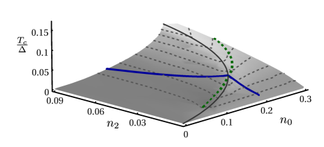
Figure 4: The superconducting transition temperature is plotted against the occupancy of the empty, $n_{0}$ and doubly occupied, $n_{2}$ states, showing that $T_{c}$ typically increases with increasing mixed valency. The black line indicates the maximal $T_{c}$, where $T_{1}^{*}=T_{2}^{*}$, and its curve is due to the d-wave nature of the second channel. Two different physical paths are shown: (1) The cost of doubly occupancy, $U_{12}=E_{2}-E_{0}-2|\epsilon_{f}|$ is tuned while fixing the $f$-level, $\epsilon_{f}$ (blue, solid path). Here, $E_{0}$ is fixed and $E_{2}$ increases from left to right. (2) Alternatively, the hybridization, $V$ can be increased, as by pressure or by exchanging $4f$ for $5f$ ions (green, dashed path). $T_{c}$ is scaled by $\Delta=\pi V_{1}^{2}$, and we have fixed $n_{c}=1.8$ in units of $N/2$.

Note that in the full model, the Kondo temperatures $T_{1}^{*}$ and $T_{2}^{*}$ mark crossovers into the heavy Fermi liquids. The appearance of phase transitions associated with condensation of $\langle b_{1}\rangle$ and $\langle b_{2}\rangle$ here is a spurious consequence of the mean-field large-$N$ treatment and is resolved with $1/N$ corrections coleman83 . However, the superconducting phase transition is not spurious and will survive to finite $N$.

In Figure 4, we plot the superconducting transition temperature versus the proportion of empty states, $n_{0}=b_{0}^{2}$ and that of doubly occupied states, $n_{2}=b_{2}^{2}$. Larger $n_{0}$ and $n_{2}$ indicate a greater degree of mixed valency, which may be obtained by varying $V$, $E_{0}$ and $E_{2}$. We show two possible paths for tuning real materials: (1) By varying $U_{12}$, $E_{2}=\epsilon_{f}+U_{12}$ will change, while $E_{0}$ remains fixed. This path is qualitatively identical to that of the two channel Kondo model when $J_{2}/J_{1}$ is varied: there is a superconducting dome with maximal $T_{c}$ where $T_{1}^{*}=T_{2}^{*}$; (2) By changing the hybridization, $V$ and keeping $E_{0}/E_{2}$ fixed, $T_{c}$ can increase monotonically with increasingly mixed valence, as it does between CeCoIn₅ and PuCoGa₅. A similar increase slightly away from the maximal $T_{c}$ can explain the non-monotonic change in $T_{c}$ with increasing pressure in CeCoIn₅[sidorov02, ].

V Charge Redistribution

As the development of composite pairing mixes the empty and doubly occupied states, each develops a non-zero occupation, and the charge density changes. The link between the $f$-electron charge and the development of the Kondo effect in the one-channel Anderson model was explored by Gunnarsson and Schoenhammergunnarsson83 , who showed that the $f$-electron valence, $n_{f}$ decreases gradually with temperature through the Kondo crossover, $n_{f}(T)=1-b_{0}^{2}(T)$. The mixing of the empty and doubly occupied states adds a new element to this relationship, and the consideration of real, non-$s$-wave hybridizations allows us to explore the higher angular momentum components of the charge distribution. The charge density can be written, $\hat{\rho}({\bf{x}})=\hat{\psi}^{\dagger}_{\alpha}({\bf{x}})\hat{\psi}_{\alpha}({\bf{x}})$, where $\hat{\psi}^{\dagger}_{\alpha}({\bf{x}})$ creates a physical electron of spin $\alpha$ at ${\bf{x}}$. The electron field ${\bf{x}}$ can be approximately decomposed as a superposition of two orbitals $\Gamma_{1}$ and $\Gamma_{2}$ at nearby lattice sites $j$,

$$\hat{\psi}_{\alpha}({\bf{x}})\!=\!\sum_{j}\left[\Phi_{1}\right]_{\alpha\beta}\!({\bf{x}}-{\bf{R}}_{j})\hat{f}_{1j\beta}+\left[\Phi_{2}\right]_{\alpha\beta}\!({\bf{x}}-{\bf{R}}_{j})\hat{f}_{2j\beta},$$ (90)

where we have reintroduced the spin-orbit form factor, $[\Phi_{\Gamma}]_{\alpha\beta}$ in order to model real materials. The charge density of an $f$-electron located at the origin in channel $\Gamma$ is $\rho_{\Gamma}({\bf{x}})={\hbox{Tr}}|\Phi_{\Gamma}({\bf{x}})|^{2}R({\bf{x}})^{2}$, where $R({\bf{x}})$ is the radial function for the $f$-electron, and $|\Phi_{\Gamma}({\bf{x}})|^{2}$ is a diagonal matrix. If we assume that the overlap of electrons at neighboring sites is negligible, the total charge density has three different terms,

$$\hat{\rho}({\bf{x}}) = \sum_{j}\rho_{1}({\bf{x}}-{\bf{R}}_{j})f_{1j\beta}^{\dagger}f_{1j\beta}+\rho_{2}({\bf{x}}-{\bf{R}}_{j})f_{2j\beta}^{\dagger}f_{2j\beta}$$ (93)

$$+\left[\Phi_{1}^{\dagger}\Phi_{2}\right]_{\alpha\beta}({\bf{x}}-{\bf{R}}_{j})f_{1j\alpha}^{\dagger}f_{2j\beta}+\mathrm{h.c.},$$

where we have kept the spin indices of $\left[\Phi_{1}^{\dagger}\Phi_{2}\right]_{\alpha\beta}$, as it may not be diagonal in spin space. In terms of the Hubbard operators, we can replace,

$$f^{\dagger}_{1j\beta}f_{1j\beta} = X_{22}(j)+n_{s}(j)=B_{2j}^{\dagger}B_{2j}+n_{s}(j)$$ (94)

$$f^{\dagger}_{2j\beta}f_{2j\beta} = X_{22}(j)+X_{\Gamma_{2}\beta\Gamma_{2}\beta}(j)=B_{2j}^{\dagger}B_{2j}+\gamma^{\dagger}\gamma$$ (95)

$$f^{\dagger}_{1j\alpha}f_{2j\beta} = X_{\Gamma_{1}\alpha\Gamma_{2}\beta}(j),$$ (96)

where as before, the number of singly occupied states on site $j$, $n_{s}(j)=N/2-B_{0j}^{\dagger}B_{0j}-B_{2j}^{\dagger}B_{2j}$, and $\gamma^{\dagger}=B_{0}^{\dagger}(-i\sigma_{2})[B_{2}^{\dagger}]^{T}=b_{0}^{\dagger}a_{2}^{\dagger}+b_{2}^{\dagger}a_{0}^{\dagger}$ is the operator from equation (55), so that $\gamma^{\dagger}f_{\alpha}^{\dagger}$ creates an electron in the excited single-electron crystal field state $|\Gamma_{2}\alpha\rangle$, see Fig. 3. The third term, $X_{\Gamma_{1}\alpha;\Gamma_{2}\beta}=|\Gamma_{1},\alpha\rangle\langle\Gamma_{2},\beta|$ mixes the two crystal field states, shifting charge from $\Gamma_{1}$ to $\Gamma_{2}$. In the large-$N$ mean-field theory, this state corresponds to non-vanishing diagonal elements of the matrix $\langle\mathcal{A}_{2}^{\dagger}\mathcal{A}_{0}\rangle$ in Eq. (66), $\langle X_{\Gamma_{1}\alpha\Gamma_{2}\beta}\rangle\sim a_{0}b_{2}+a_{2}b_{0}$. Since $\Gamma_{1}$ and $\Gamma_{2}$ are two different representations of the crystal point group, such mixing implies that the crystal symmetry is spontaneously broken: in Ce-115 materials it would correspond to orthorhombic “nematic” density wave state, which has not been observed. We are primarily interested in superconducting instability, and therefore ignore such a state by setting $a_{2}=0$ in what follows, assuming we have already gauge fixed $a_{0}=0$. Any occupation of the excited crystal field state, $\langle X_{\Gamma_{2}\beta\Gamma_{2}\beta}\rangle$ is also eliminated by this Ansatz.

In the heavy Fermi liquid and superconducting states, we may use the constraint to rewrite $f^{\dagger}_{1j\beta}f_{1j\beta}=N/2-X_{00}(j)$. The charge distribution becomes,

$$\hat{\rho}({\bf{x}})\!=\!\!\sum_{j}\!\rho_{1}({\bf{x}}\!-\!{\bf{R}}_{j}\!)\!\!\left[\!\frac{N}{2}\!\!-\!\!X_{00}(j)\!\right]\!\!+\!\rho_{2}({\bf{x}}\!-\!{\bf{R}}_{j}\!)X_{22}(j).$$ (97)

Integrating this charge density around a single site gives us the $f$-electron valence, $n_{f}=1-b_{0}^{2}+b_{2}^{2}$, which we plot as a function of $T$ in Figure 5 for two different $E_{2}/E_{0}$. The phase transition at $T^{*}$ is an artifact of the large $N$ limit and becomes a crossover for any finite $N$, but the sharp kink in $n_{f}$ at the superconducting transition temperature remains for all $N$. Experimentally determining the $f$-electron valence may be possible using core-level valence spectroscopy for Ce compounds or the Mössbauer isomer shift for NpPd₅Al₂, where current measurements do indicate a small, positive change in the isomer shift through $T_{c}$ [gofryk09, ]. If Np is in the $5f^{3}$ valence state, with dominant fluctuations between $5f^{3}\rightleftharpoons 5f^{4}$, then the isomer shift will increase with decreasing temperature down to $T_{c}$, where it will begin to decrease sharply as $5f^{2}$ states mix in, as the black curve in Figure 5 shows. Experimentally, the isomer shift was measured at 10K, well above $T_{c}$ and then below $T_{c}$, so the observed positive shift could just be due to the increase above $T_{c}$, and further measurements are necessary. The clear observation of a sharp negative shift precisely at the superconducting transition temperature would indicate the presence of composite pairing.

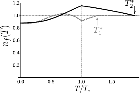
Figure 5: The $f$-electron valence, $n_{f}$ changes as the Kondo effect and composite pair superconductivity develop. Two examples are shown - the black curve has $T_{2}^{*}>T_{1}^{*}$, as expected for NpPd₅Al₂, so that the valence increases below $T_{2}^{*}$, and then sharply decreases for $T<T_{c}$. For the dashed gray curve, $T_{1}^{*}>T_{2}^{*}$, as expected for Ce$M$In₅ and a sharp increase in the valence is seen at $T_{c}$. The sharp kinks at $T^{*}_{1},T^{*}_{2}$ are artifacts of the mean field calculation, becoming smooth crossovers in real materials, while the superconducting kinks should be observable in real materials.

As superconductivity develops, the occupation of the doubly occupied state acquires an expectation value, leading to an increase in the $\Gamma_{2}$ charge density. This redistribution of the $f$-electron charge results in a quadrupole moment associated with superconductivity. Again, since the development of superconductivity is a phase transition, the quadrupole moment changes sharply at $T_{c}$. The quadrupole charge component has an indirect effect on the superconducting transition temperature through its linear coupling to strain, leading to a linear dependence of $T_{c}$ on the tetragonal strain, $c/a$. Such a linear increase of $T_{c}$ with $c/a$ has been observed in both the Ce and Pu 115s, although it is conventionally attributed to dimensionality effectsbauer04 . The quadrupole moment of the composite condensate provides an alternate explanation, and, in addition, leads to the development of electric field gradients around the $f$-lattice sites, which can also be measured directly as a shift in the nuclear quadrupole resonance frequency, $\Delta\nu_{NQR}$ at the nuclei of the nearby atoms.

To make contact with potential experiments, we examine CeCoIn₅ in more detail. ¹¹⁵In atoms have a nuclear moment $I=9/2$, which results in a quadrupole moment, $Q=8.3\times 10^{-29}\text{m}^{2}$, making them NQR activeurbano10 . The symmetry of the ground state doublet is $\Gamma_{7}^{+}$[christianson04, ], whose angular dependence is given by,

$$|\Phi_{\Gamma_{7}^{+}}|^{2}(\theta,\phi) = \frac{3}{16}\sin^{2}\theta\left[2\sqrt{5}\cos 4\phi\sin^{2}\theta\sin 2\xi\right.$$

$$+ \left.11+6\cos 2\xi+5\cos 2\theta(1+2\cos 2\xi)\right]$$

where $\xi$ is a crystal-field parameter depending on the microscopic details that can be measured with inelastic neutron scattering, and we set $\xi\approx.25$ for CeCoIn₅ [christianson04, ]. We take the symmetry of the second channel to be $\Gamma_{2}=\Gamma_{6}$, whose angular dependence is,

$$|\Phi_{\Gamma_{6}}|^{2}(\theta,\phi)=\frac{3}{32}\left[12\cos 2\theta+5(3+\cos 4\theta)\right].$$ (99)

We can now use the real charge distributions of the two orbitals to estimate the magnitude of the electric field gradient, $V_{ab}=-\partial E_{a}/\partial x_{b}$, where

$$\rho_{\Gamma}({\bf{x}})=|\Phi_{\Gamma}|^{2}(\theta,\phi)R(r)^{2}.$$ (100)

$R(r)$ is the $4f$ radial function,

$$R(r)=\frac{1}{96\sqrt{35}}\left(\frac{Z^{3/2}r}{2a_{B}}\right)^{3}\exp\left(-\frac{Zr}{4a_{B}}\right).$$ (101)

$a_{B}=.53$Å  is the Bohr radius, and $Z=6\sqrt{10}a_{B}/r_{Ce}$ is adjusted so that the atomic radius is that of Ce³⁺, $\langle r\rangle=r_{Ce}=1.15$ Å[bringer83, ].

The NQR frequency measures the electric field gradients at two different indium sites in the crystal: the in-plane, high symmetry In(1) sites, which sit in the center of a square of Ce atoms, and the lower symmetry out-of-plane In(2) sites, which are above and in-between two Ce atoms. The NQR frequency is given bywhite79 ,

$$\nu_{NQR}=\frac{3eV_{zz}Q}{2hI(2I-1)}\mathrm{Hz}.$$ (102)

At the In(2) site, there is a nonzero asymmetric contribution, $\eta=|V_{xx}-V_{yy}|/V_{zz}$, which can be independently determined from experiment. Now that we have an accurate expression for the charge distribution of the two orbitals, we may calculate the electric field gradient at ${\bf{x}}$ associated with a charge $q$ in orbital $\Gamma$ at ${\bf{R}}_{j}$:

$$\!\!\!\!\!\!\!V_{aa}^{\Gamma}({\bf{x}},{\bf{R}}_{j}\!)\!=\!\frac{q}{4\pi\epsilon_{0}}\!\!\int_{{\bf{x}}^{\prime}}\!\!\!\rho_{\Gamma}({\bf{x}}^{\prime}\!-\!{\bf{R}}_{j}\!)\!\left[\!\frac{3(\!a\!-\!a^{\prime})^{2}}{|{\bf{x}}\!-\!{\bf{x}}^{\prime}|^{5}}\!-\!\frac{1}{|{\bf{x}}\!-\!{\bf{x}}^{\prime}|^{3}}\!\!\right]\!.$$ (103)

Summing over the eight neighboring Ce sites is sufficient to estimate the magnitude of the NQR shift, where we use the lattice constants of CeCoIn₅, $a=4.6$Å, and $c=7.4$Å[petrovic01a, ]. The electric field gradients for a charge $eq_{\Gamma}$ in channel $\Gamma$ are shown in Table I.

CeCoIn5	In(1) $V_{zz}$	In(2) $V_{zz}$
$\Gamma_{7}^{+}$	$-1.5q_{7+}\cdot 10^{20}$ V/m2	$+5.0q_{7+}\cdot 10^{19}$ V/m2
$\Gamma_{6}$	$+1.4q_{6}\cdot 10^{20}$ V/m2	$-3.6q_{6}\cdot 10^{19}$ V/m2

Table 1: Estimated electronic field gradients at the two In sites in CeCoIn₅ due to $eq_{\Gamma}$ charge in the $f$-electron orbital, $\Gamma=\Gamma_{7}^{+},\Gamma_{6}$, where $e$ is the charge of an electron.

For equal channel strengths, the total charge of the $f$-ion remains unity, and the increasing occupations of the empty and doubly occupied sites cause holes to build up with symmetry $\Gamma_{7}^{+}$ and electrons with symmetry $\Gamma_{6}$, $q\equiv q_{6}=-q_{7+}$. If we define $q(T)$ to be the temperature dependent occupation of the empty/doubly occupied states, in the mean field $q(T)=\langle b_{0}^{2}\rangle=\langle b_{2}^{2}\rangle$ will be proportional to $T_{c}-T$ just below $T_{c}$, and we can define,

$$q(T)=q_{0}\frac{T_{c}-T}{T_{c}},$$ (104)

where $q_{0}$ is the ground state occupation of the empty/doubly occupied states. In terms of $q_{0}$, the superconducting NQR frequency shift will be,

$$\Delta\nu_{NQR}^{1}(T) = -7.6q_{0}\frac{(T_{c}-T)}{T_{c}}\mathrm{kHz}$$ (105)

$$\Delta\nu_{NQR}^{2}(T) = +11q_{0}\frac{(T_{c}-T)}{T_{c}}\mathrm{kHz}$$ (106)

Even assuming a reasonably large $5$% change in the single-occupancy ($q_{0}=.05$) for CeCoIn₅ with $T_{c}=2.3$K will lead to a small shift in $\nu_{NQR}^{1,2}$ with a slope of $\approx-.16,+.24$ kHz/K, beginning precisely at $T_{c}$. We could also consider the case of unequal channel strengths, where the Ce exchanges charge with the conduction electrons, sitting in the In $p$-orbitals, however this term will be similarly small in any clean sample. If this shift could be distinguished, it would be an unambiguous signal of composite pairing. As this shift is quite small, Mössbauer spectroscopy, which directly probes the $f$-ions may be a more likely technique to observe the development of a condensate quadrupole moment. Given that the crystal fields for NpPd₅Al₂ are unknown, we can only make a rough estimate of the magnitude of the quadrupolar splitting, following [potzel93, ]. The $f$-ion contribution to the splitting will originate from a redistribution of charge $eq$ within the $f$-orbitals, and can be as large as $0.2q$ mm/s. The lattice contribution to the quadrupole splitting, which originates from the change in $f$-valence redistributing change within the lattice, will likely be a larger effect.

VI Conclusions

Our two-channel Anderson model treatment has shown how composite pairing arises as the low energy consequence of valence fluctuations in two competing symmetry channels, which in turn manifests itself as a mixing of the empty and doubly occupied states,

$$\Delta_{SC}\propto\langle|0\rangle\langle 2|\rangle.$$ (107)

Composite pairing is primarily a local phenomena, where the pairing occurs within a single unit cell. The mixing is reminiscent of an intra-atomic antiferromagnetism, involving d-wave singlet formation between the $|\Gamma_{1}\rangle$ and $|\Gamma_{2}\rangle$ states. It is the atomic physics of the $f$-ions, tuned by their local chemical environment that drives the superconductivity. Such chemically driven d-wave pairing is a fascinating direction for exploring higher temperature superconductors in even more mixed valent $3d$ materials, as the strength of the composite pairing increases monotonically with increasing valence fluctuations, which accounts for the difference in transition temperatures between the cerium and the actinide 115 superconductors, and for the effects of pressure.

The local nature of composite pairing should make it less sensitive to disorder than more conventional anisotropic pairing mechanisms. Such insensitivity is observed in the doped Ce-115 materials, where superconductivity survives up to approximately $25\%$ substitution on the Ce site paglione07 , while neither Ce-site nor In-site disorder behave according to Abrikosov-Gorkov, suggesting instead a percolative transitionbauer10 .

The redistribution of charge due to the mixing of empty and doubly occupied states provides a promising direction to experimentally test for composite pairing, which should appear as a sharp redistribution of charge associated with the superconducting transition. Both monopole ($f$-valence) and quadrupole (electric field gradients) charge effects should be observable, with core-level X-ray spectroscopy and the Mössbauer isomer shift or as a shift in the NQR frequency at surrounding nuclei, respectively. We predict a shift with slope of order $\pm 0.3$kHz/K in the NQR frequency of In nuclei in CeCoIn₅.

Deriving these results in an exact, controlled mean field theory required the introduction of symplectic Hubbard operators, which maintain the time-reversal properties of $SU(2)$ electrons in the large $N$ limit. While our results are obtained in the large-$N$ limit, it should also be possible to use these Hubbard operators to develop a dynamical mean field theory treatment of the two-channel Anderson lattice, enabling us to examine composite pairing for $N=2$.

In addition to the two-channel Anderson model, the development of symplectic-Hubbard operators allows a controlled treatment of the finite-$U$ Anderson model, which is potentially useful as an impurity solver for dynamical mean field theory. We identify the finite-$U$ model as a special case of our two channel model when the electron and hole fluctuations occur in the same symmetry channel, $\Gamma_{1}=\Gamma_{2}$. At first sight, this model appears to give s-wave superconductivity, however, the $SU(2)$ constraint, $\lambda_{1}$ forbids any on-site pairing and completely kills the superconductivity, leaving only the simple Fermi liquid solution. We expect $1/N$ corrections to this mean field limit will differ from the $SU(N)$ approach, and an interesting future direction is to use the Gaussian fluctuations to examine the charge fluctuation side peaks.

Acknowledgements. We should like to acknowledge discussions with Cigdem Capan, Maxim Dzero, Zachary Fisk, Pascoal Pagliuso and Ricardo Urbano. This work was supported by the National Science Foundation, Division of Materials Research grant DMR 0907179.

References

(1)N. D. Mathur, F. M. Grosche, S. R. Julian,
I. R. Walker, D. M. Freye,R. K. W. Haselwimmer and G. G. Lonzarich,
Nature 394 39, (1998).
(2) C. Petrovic et al., J. Phys.: Condens. Matter 13, L337(2001).
(3)D. Aoki et al., J. Phys. Soc. Jpn., 76, 063701-063704 (2008).
(4) J. L. Sarrao et al., Nature (London) 420, 297-299 (2002).
(5)T. Willers, Z. Hu, N. Hollmann, P. O. Korner,
J. Gegner, T. Burnus, H. Fujiwara, A. Tanaka, D. Schmitz, H. H. Hsieh,
H.-J. Lin, C. T. Chen, E.D. Bauer, J.L.Sarrao, E. Goremychkin,
M. Koza, L. H. Tjeng and A. Severing, Phys. Rev. B 81, 195114 (2010).
(6) K Gofryk, J Griveau, E Colineau, J. P. Sanchez,
J. Rebizant, and R. Caciuffo, Physical Review B 79, 134525 (2009).
(7) R. Flint, M. Dzero and P. Coleman, Nat. Phys. 4, 643 (2008).
(8) R. Flint and P. Coleman, Phys. Rev. Lett. 105, 246404(2010).
(9) E. Abrahams, A. Balatsky, D.J. Scalapino and J. R. Schrieffer, Phys. Rev. B 52, 1271(1995).
(10)P. G. Pagliuso et al.: Phys. Rev. B 64 (2001) 100503; P. G. Pagliuso et al.: Physica B 312 (2002) 129.
(11) H. Shishido et al., J. Phys. Soc. Jap. 7, 162–173(2002).
(12) P. Coleman, A. M. Tsvelik, N. Andrei and H. Y. Kee, Phys. Rev. B 60, 3608 - 3628 (1999).
(13) J. Hubbard, Proc. Royal Soc. London A, 277 237 (1964).
(14) C. J. Bolech and N. Andrei, Phys. Rev. Lett. 88, 237206-237210, (2002).
(15) I. Affleck, Z. Zou, T. Hsu and P. W. Anderson, Phys. Rev. B 38, 745, (1988).
(16) X.G. Wen and P.A. Lee, Phys. Rev. Lett. 76, 503 (1996).
(17) P. Coleman, Phys. Rev. B 28, 5255 (1983).
(18) H. Keiter and J.C. Kimball, Int J. Magn. 1, 233 (1971).
(19) K. Haule and G. Kotliar, Nat. Phys. 5, 796 - 799 (2009).
(20) P. W. Anderson, Phys. Rev. Lett. 34, 953 (1975).
(21) P. Morel and P.W. Anderson, Phys. Rev. 125, 1263 (1962).
(22) O. Gunnarsson & K. Schonhammer, Phys. Rev. B 28, 4315(1983).
(23) Bauer, E.D., et al., Phys. Rev. Lett. 93, 147005 (2004).
(24) R. Urbano (private communication).
(25)A. D. Christianson et al., PRB 70, 134505(2004).
(26) A. Bringer, Solid State Comm. 46, 591(1983).
(27) R.M. White and T. H. Geballe, “Long Range Order in Solids” p.193-194 (Academic Press, New York, 1979).
(28) W.Potzel, G.M. Kalvius, and J.Gal, in Handbook on the Physics and Chemistry of Rare Earths, edited by K.A. Gschneider, Jr., L. Eyring, G.H. Lander, and G.R. Chopin (Elsevier, Amsterdam, 1993), Vol. 17,p.539.
(29)J. P. Paglione, T. A. Sayles, P. C. Ho,
J. R. Jeffries and M. B. Maple, Nature Physics 3, 703 (2007).
(30)E. D. Bauer, Yi-feng Yang, C. Capan,
R. R. Urbano, C. Miclea, H. Sakai, F. Ronning, M. J. Graf,
A. V. Balatsky, R. Movshovich, A. D. Bianchi, A. P. Reyes,
P. L. Kuhns, J. D. Thompson, and Z. Fisk, PNAS 108, 6857 (2011).
(31) V.A. Sidorov et al, Phys. Rev. Lett. 89,157004 (2002).