Quantum quench dynamics of the Bose-Hubbard model at finite temperatures

Abstract

We study quench dynamics of the Bose-Hubbard model by exact diagonalization. Initially the system is at thermal equilibrium and of a finite temperature. The system is then quenched by changing the on-site interaction strength $U$ suddenly. Both the single-quench and double-quench scenarios are considered. In the former case, the time-averaged density matrix and the real-time evolution are investigated. It is found that though the system thermalizes only in a very narrow range of the quenched value of $U$, it does equilibrate or relax well in a much larger range. Most importantly, it is proven that this is guaranteed for some typical observables in the thermodynamic limit. In order to test whether it is possible to distinguish the unitarily evolving density matrix from the time-averaged (thus time-independent), fully decoherenced density matrix, a second quench is considered. It turns out that the answer is affirmative or negative according to the intermediate value of $U$ is zero or not.

I Introduction

Out-of-equilibrium dynamics following a quantum quench is a topic of intense study at present. The theme is pursued primarily along two lines. The first one is about the equilibration and thermalization mechanism of a quantum system bloch11 ; rigol_09 ; rigol_integrable ; rigol_nature ; manmana ; roux09 ; roux2 ; kollath07 ; weiss ; hanggi , a fundamental yet still open issue in statistical physics. The second one is about the the real-time dynamical behavior of a many-body system greiner ; sengupta ; luttinger ; dimer ; polkovnikov , which is highly non-trivial in the regime where the quasi-particle picture breaks down.

Among all the models investigated so far, the Bose-Hubbard model takes a special position. As a paradigmatic strongly-correlated model, it can be realized accurately with cold atoms in optical lattices, and especially, the parameters can be controlled (e.g. changed suddenly) to a high degree zoller ; bloch ; bloch_np . This nice property makes it an ideal candidate to investigate quantum quench dynamics both theoretically and experimentally. Up to now, in the few theoretical works on the quench dynamics of the Bose-Hubbard model roux09 ; roux2 ; kollath07 ; dimer ; sengupta , the state of the system before the quench is always assumed to be the ground state of the initial Hamiltonian. That is, the system is assumed to be at zero temperature initially. However, in this paper we shall start from a thermal equilibrium state. One should note that this scenario is actually more experimentally relevant. Because in current experiments, one generally gets not a single tube of cold atoms, but instead a two-dimensional array of one-dimensional lattices for the cold atoms bloch_np . In other words, an ensemble of one-dimensional Bose-Hubbard models is obtained in one shot. Moreover, in view of the fact that the cold atoms are at finite temperatures necessarily qi ; zhou , it is reasonable to start from a thermal state described by a canonical ensemble density matrix [see Eq. (2) below].

As emphasized by Linden et al. linden , in the pursuit of thermalization, it is important to distinguish the two closely related but inequivalent concepts of equilibration and thermalization. The latter is much stronger and has the trademark feature of the Boltzmann distribution, whereas the former refers only to the stationary property of the density matrix of a (sub)system or some physical observables. It is highly possible that a system equilibrates but without thermalization. This is actually the case for the Bose-Hubbard model. As revealed both in previous works (zero temperature case) roux09 ; kollath07 and in the present paper (finite temperature case), the Bose-Hubbard model thermalizes only if the quench amplitude is not so large, at least at the finite sizes currently accessible. However, it will be shown below that in a much wider range of parameters, some generic physical observables equilibrate very well. Among them are the populations on the Bloch states, which are ready to measure by the typical time-of-flight experiment rmp . Remarkably, this is actually guaranteed for these quantities in the thermodynamic limit, i.e., when the size of the system gets large enough.

The equilibration behavior of the physical observables imposes a question. It is ready to recognize that the equilibration of the physical observables is largely an effect of interference cancelation. It never means that the density matrix has suffered any dephasing or decoherence. Actually, the density matrix evolves unitarily and in the diagonal representation of the Hamiltonian, its elements simply rotate at constant angular velocities. A natural question is then, does the time-dependence of the density matrix has any chance to exhibit it, given that it is almost absent in the average values of the physical observables? This leads us to consider giving the system a second quench. The concern is, would the system yield different long-time behaviors if the second quench comes at different times? It turns out that the answer depends on whether the intermediate Hamiltonian is integrable or non-integrable. In the former case, the density matrix shows repeated appreciable recurrences and thus the dependence on the second quench time is apparent. In the latter case, on the contrary, the density matrix shows no sign of recurrence and quantitatively similar long-time dynamics is observed for quenches at different times.

This paper is organized as follows. In Sec. II, the setting of the problem and the basic approaches are given. In Sec. III, the dynamics after a single quench is studied. The time-averaged density matrix and the real-time evolution of some physical observables are investigated in detail. Based on the observation in this Section, we proceed to study the scenario of a second quench in Sec. IV. Finally, we summarize the results in Sec. V.

II Basic formalism

The time-dependent Hamiltonian of the Bose-Hubbard model is ($\hbar=k_{B}=1$ throughout this paper)

$$H(t)=-J\sum_{l=1}^{M}(a_{l}^{\dagger}a_{l+1}+a_{l+1}^{\dagger}a_{l})+\frac{U(t)}{2}\sum_{l=1}^{M}a_{l}^{\dagger}a_{l}^{\dagger}a_{l}a_{l}.$$ (1)

Here $M$ is the number of sites (the total atom number will be denoted as $N$) and $a_{l}^{\dagger}$ ($a_{l}$) is the creation (annihilation) operator for an atom at site $l$. Note that here periodic boundary condition is assumed. The parameters $J$ and $U$ are the nearest-neighbor hopping strength and the on-site atom-atom interaction strength, respectively. Note that the dynamics of the system depends only on the ratio $U/J$, thus we will set $J=1$ throughout. We say the system is quenched if $U$ is changed suddenly at some time from one value to another value. Experimentally, for cold atoms in an optical lattice, this can be realized by using the Feshbach resonance.

Assume that initially the parameter $U$ is of value $U_{i}$ (the corresponding Hamiltonian is denoted as $H_{i}$), and the system is at thermal equilibrium and of inverse temperature $\beta_{i}=1/T_{i}$. Denote the $m$-th eigenvalue and eigenstate of $H_{i}$ as $E_{m}^{i}$ and $|\psi_{m}^{i}\rangle$, respectively. The initial density matrix of the system is then

$$\rho_{i}=\frac{1}{Z_{i}}\exp(-\beta_{i}H_{i})=\sum_{m=1}^{D}p^{i}_{m}|\psi_{m}^{i}\rangle\langle\psi_{m}^{i}|,$$ (2)

where $Z_{i}=\sum_{m=1}^{D}\exp(-\beta_{i}E_{m}^{i})$ is the partition function and $p^{i}_{m}=\frac{1}{Z_{i}}\exp(-\beta_{i}E^{i}_{m})$ is the probability of occupying the eigenstate $|\psi_{m}^{i}\rangle$. Note that $D=\frac{(M+N-1)!}{(M-1)!N!}$ is the dimension of the Hilbert space $\mathcal{H}$. The density matrix at time $t$ is given formally as $\rho(t)=U(t)\rho_{i}U^{\dagger}(t)$, with $U(t)=\mathcal{T}\exp[-i\int_{0}^{t}d\tau H(\tau)]$. Here $\mathcal{T}$ means time ordering.

The Hamiltonian $H(t)$ is invariant under the translation $(a_{l},a_{l}^{\dagger})\rightarrow(a_{l+1},a_{l+1}^{\dagger})$. This indicates that the total quasi-momentum of the system $q=\sum_{k=0}^{M-1}ka_{k}^{\dagger}a_{k}\pmod{M}$, where $a_{k}^{\dagger}=\frac{1}{\sqrt{M}}\sum_{l=1}^{M}\exp(i2\pi kl/M)a_{l}^{\dagger}$ is the creation operator for an atom in the $k$-th Bloch state, is conserved. This property implies that if the full Hilbert space is decomposed into $M$ subspaces according to the values of $q$, i.e., $\mathcal{H}=\oplus_{q=0}^{M-1}\mathcal{H}^{(q)}$, the Hamiltonian and the density matrix are always block-diagonal with respect to the $q$-subspaces, i.e.,$H(t)=\oplus_{q=0}^{M-1}H^{(q)}(t)$ and $\rho(t)=\oplus_{q=0}^{M-1}\rho^{(q)}(t)$ zjm ; zjm2 . It is then possible to study the dynamics in each subspace individually (which saves a lot of computational resource) and then gather the information together (note that for the expectation values of quantities like $a_{k}^{\dagger}a_{k}$, there are contributions from each subspace). Here it is necessary to mention that though we should have done the gathering or averaging process for many quantities studied below, we would rather not do so, because it is observed that the system behaves quantitatively similar in all the $q$-subspaces beta . A single $q$-subspace captures the overall behavior very well. Therefore, our strategy is to focus on some specific $q$-subspace ($q=1$ actually) and take the normalization $tr(\rho^{(q)}(t))=1$. It is understood that in the following all Hamiltonians, density matrices, eigenvalues, and eigenstates refer to those belonging to this specific $q$-subspace. We will drop the superscript $q$ for notational simplicity.

III A single quench

Suppose at time $t=0$ the system is quenched by changing the value of $U$ from $U_{i}$ to $U_{f_{1}}$, which is then held on forever. The Hamiltonian later will be denoted as $H_{f_{1}}$, and the eigenvalues and eigenstates associated will be denoted as $E^{f_{1}}_{n}$ and $|\psi^{f_{1}}_{n}\rangle$, respectivley. In the representation of $\{|\psi^{f_{1}}_{n}\rangle\}$, the density matrix at time $t$ is then simply (in this paper $\langle\cdots\rangle$ means quantum state averaging while $\overline{\cdots}$ means time averaging)

$$\rho(t)=\sum_{m,n=1}^{D_{q}}e^{-i(E^{f_{1}}_{m}-E^{f_{1}}_{n})t}\langle\psi^{f_{1}}_{m}|\rho_{i}|\psi^{f_{1}}_{n}\rangle|\psi^{f_{1}}_{m}\rangle\langle\psi^{f_{1}}_{n}|,$$ (3)

where $D_{q}\simeq D/M$ is the dimension of the specific $q$-subspace. It will prove useful to define the time-averaged density matrix

$$\bar{\rho} = \lim_{T\rightarrow\infty}\frac{1}{T}\int_{0}^{T}dt\rho(t)$$ (4)

$$= \sum_{\begin{subarray}{c}m,n=1\\ E^{f_{1}}_{m}=E^{f_{1}}_{n}\end{subarray}}^{D_{q}}\langle\psi^{f_{1}}_{m}|\rho_{i}|\psi^{f_{1}}_{n}\rangle|\psi^{f_{1}}_{m}\rangle\langle\psi^{f_{1}}_{n}|.$$

The time-averaged density matrix is of great relevance for our purposes. First, it is both time-independent and variable-independent. Second, the time-averaged value of an arbitrary operator $O$ is given simply by $\overline{\langle O\rangle}\equiv\lim_{T\rightarrow\infty}\frac{1}{T}\int_{0}^{T}tr(\rho(t)O)dt=tr(\bar{\rho}O)$. That is, the time-averaged density matrix contains the overall information of the dynamics of the system. Actually, as we will see later, for some quantities which fluctuate little in time, the time-averaged density matrix tells almost a complete story. Third, the process of averaging over time is a process of relaxation in the sense that the entropy associated with $\bar{\rho}$ is definitely no less than that with the density matrix at an arbitrary time, i.e., $S(\bar{\rho})\geq S(\rho(t))=S(\rho_{i})$. This is a corollary of the Klein inequality chuang and is reasonable since $\rho_{i}$ contains all the information of $\bar{\rho}$ while the inverse is invalid. The equality also means that $\rho(t)$ will never be damped, and time-averaging is essential.

Note that when $U_{f_{1}}\neq 0$, generally there is no degeneracy between the eigenvalues of $H_{f_{1}}$. Therefore the time-averaged density matrix is simply diagonal in the basis of $\{|\psi^{f_{1}}_{n}\rangle\}$, i.e.,

$$\bar{\rho} = \sum_{m=1}^{D_{q}}\langle\psi^{f_{1}}_{m}|\rho_{i}|\psi^{f_{1}}_{m}\rangle|\psi^{f_{1}}_{m}\rangle\langle\psi^{f_{1}}_{m}|$$ (5)

$$\equiv \sum_{m=1}^{D_{q}}p_{m}|\psi^{f_{1}}_{m}\rangle\langle\psi^{f_{1}}_{m}|,$$

with

$$p_{m}=\langle\psi^{f_{1}}_{m}|\rho_{i}|\psi^{f_{1}}_{m}\rangle=\frac{1}{Z_{i}}\sum_{n=1}^{D_{q}}e^{-\beta_{i}E_{n}^{i}}|\langle\psi_{n}^{i}|\psi_{m}^{f_{1}}\rangle|^{2}$$ (6)

being the population on the eigenstate $|\psi_{m}^{f_{1}}\rangle$. In the special case of $U_{f_{1}}=0$, the Hamiltonian reduces to $H_{f_{1}}=\sum_{k=0}^{M-1}\omega_{k}a^{\dagger}_{k}a_{k}$, with $\omega_{k}=-2J\cos(2\pi k/M)$. In this case, each eigenvalue is of the form $\sum_{k}n_{k}\omega_{k}$, under the constraints $\sum_{k}n_{k}=N$ and $\sum_{k}kn_{k}\equiv q\pmod{M}$, and there can be level degeneracy. However, we can always make some unitary transforms in each degenerate subspace to make sure that $\bar{\rho}$ is in the form of (5).

III.1 Time-averaged density matrix

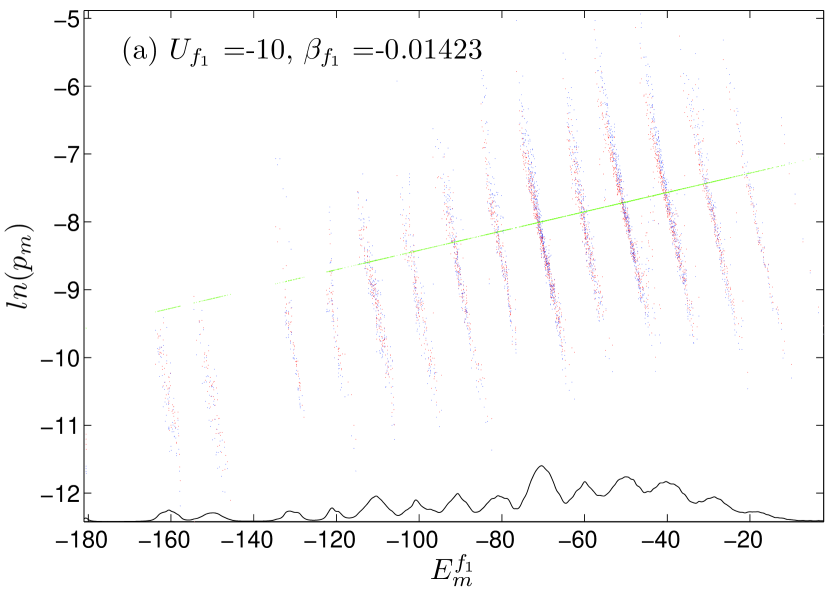
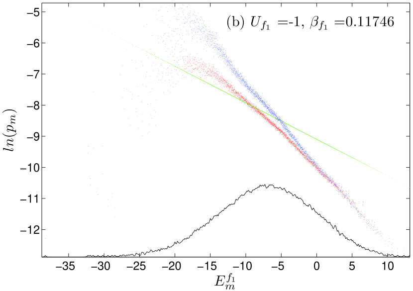
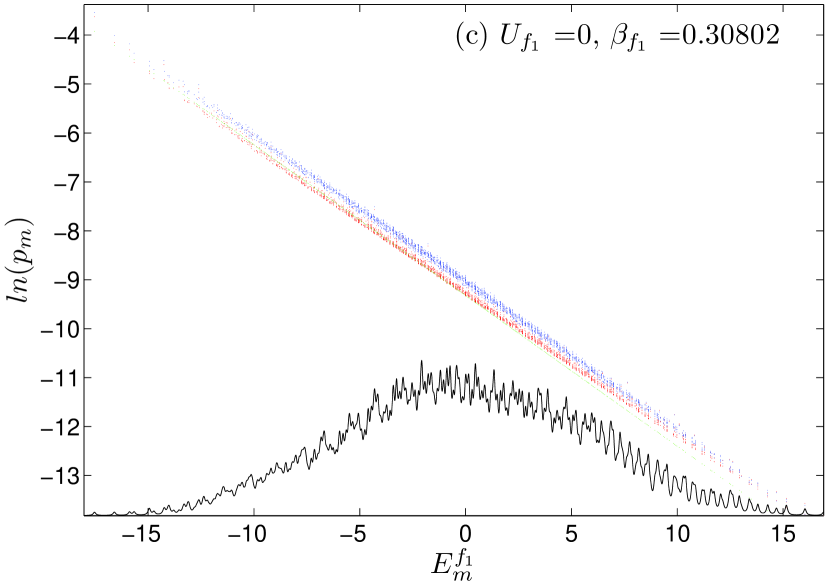
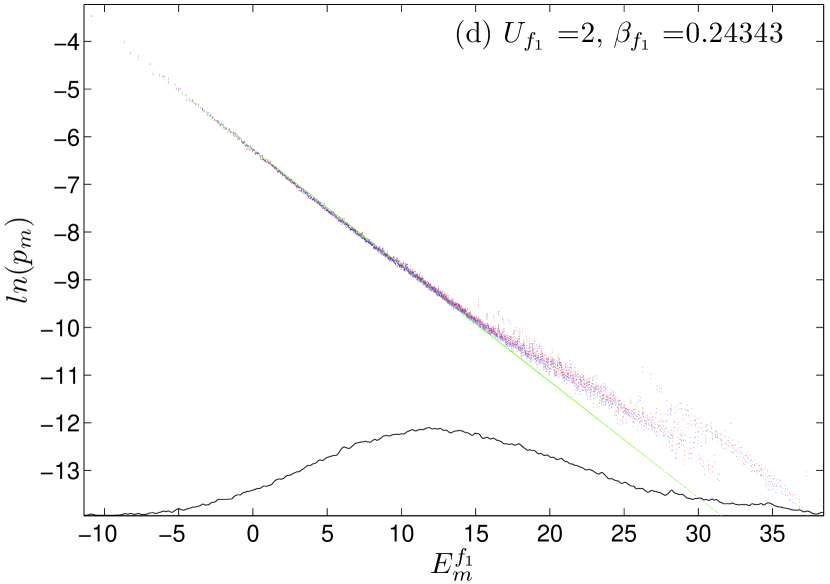
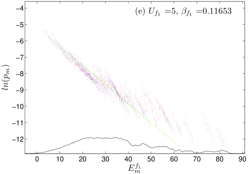
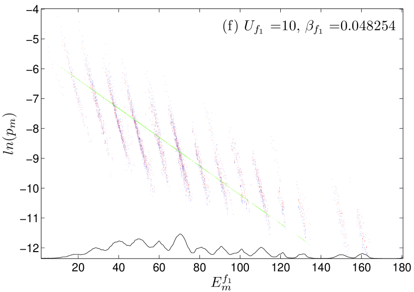
Figure 1: (Color online) Semilog plots of $p_{m}$ versus the eigenvalues $E^{f_{1}}_{m}$ (red dots). The initial state is the same for all the figures, with parameters $(M,N,q,D_{q})=(9,9,1,2700)$, $U_{i}=1$, and $\beta_{i}=0.3$. The quenched values of $U$ and the fitting inverse temperatures $\beta_{f_{1}}$ are shown in the inserts. For comparison, the data with $\rho_{c}$ (green dots) and $p^{\prime}_{m}$ (blue dots) are also shown. The black lines at the bottom depict the coarse-grained density of states of $H_{f_{1}}$ (just for reference, not corresponding to the vertical axis).

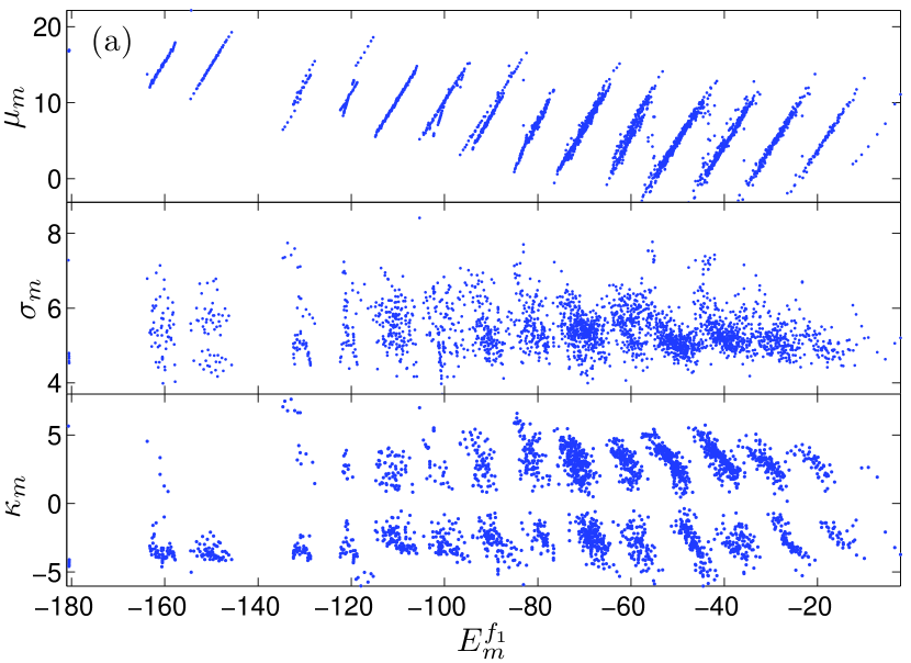
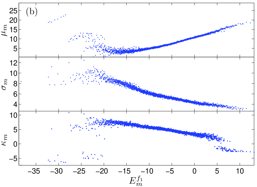
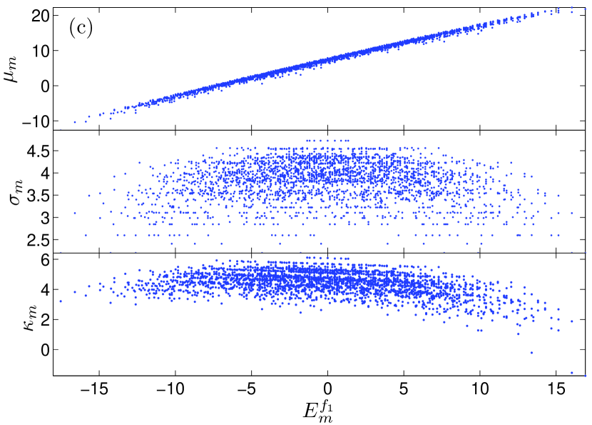
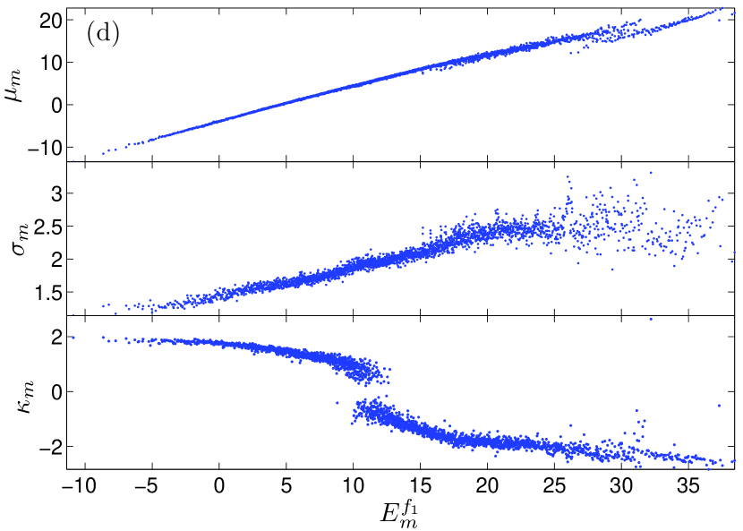
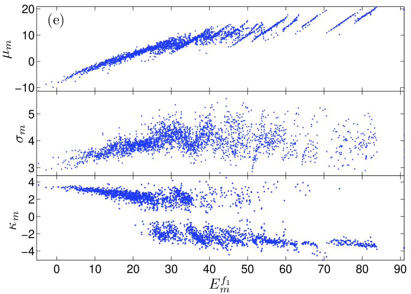
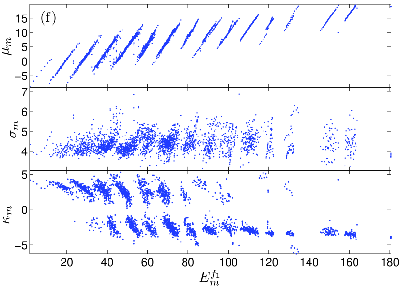
Figure 2: (Color online) The parameters $\mu_{m}$, $\sigma_{m}$, and $\kappa_{m}$ [see Eq. (9)] characterizing the probability distributions $P_{m}(E)$ associated with the eigenstates of $H_{f_{1}}$. Note that Figs. 2a-2f correspond to Figs. 1a-1f, respectively.

Since the time-averaged density matrix provides an overall information of the dynamics of the system, we look into it first. In Fig. 1, we consider the scenario of starting from the same initial condition ($U_{i}=1$, $\beta_{i}=0.3$) but quenching to six different values of $U_{f_{1}}$ negative . In each panel, the logarithms of $p_{m}$ are plotted against the eigenvalues $E^{f_{1}}_{m}$ (red dots). We have compared $\bar{\rho}$ with a canonical ensemble density matrix $\rho_{c}$, which is defined as

$$\rho_{c}=\frac{e^{-\beta_{f_{1}}H_{f_{1}}}}{tr(e^{-\beta_{f_{1}}H_{f_{1}}})}$$ (7)

under the condition $tr(\rho_{c}H_{f_{1}})=tr(\bar{\rho}H_{f_{1}})=tr(\rho_{i}H_{f_{1}})$. Here $\beta_{f_{1}}$, the final inverse temperature, is the only fitting parameter. In Fig. 1, the green dots which form a straight line correspond to $\rho_{c}$.

We see that $\bar{\rho}$ exhibits many interesting features. In the case of $U_{f_{1}}=0$, $\bar{\rho}$ agrees well with $\rho_{c}$ throughout the spectrum. In the case of $U_{f_{1}}=2$, $\bar{\rho}$ agrees well with $\rho_{c}$ in the lower part of the spectrum, while deviates from it significantly in the higher part of the spectrum. But overall the two are in good agreement since the weight of the higher part is small. The case of $U_{f_{1}}=-1$ is somewhat the reverse of the $U_{f_{1}}=2$ case. It is in the lower part of the spectrum that $\ln p_{m}$ fluctuates wildly. In the higher part $\ln p_{m}$ goes almost linearly. Since the weight is dominated by the lower part, $\rho_{c}$ is not a good approximation of $\bar{\rho}$. In the strong interaction limits of $U_{f_{1}}=\pm 10$, another feature takes the place. As a whole the red dots do not fall close to a single straight line, but they do form some stripes, and the stripes are almost parallel with a common slope close to $\beta_{i}$. It is easy to recognize that each stripe corresponds to a bump in the density of states of $H_{f_{1}}$.

In order to understand the various features in Fig. 1, we rewrite $p_{m}$ as

$$p_{m}=\frac{1}{Z_{i}}\int_{-\infty}^{+\infty}dEe^{-\beta_{i}E}P_{m}(E),$$ (8)

where $P_{m}(E)=\sum_{n}|\langle\psi_{n}^{i}|\psi_{m}^{f_{1}}\rangle|^{2}\delta(E-E_{n}^{i})$ is a probability distribution prod associated with $|\psi_{m}^{f_{1}}\rangle$. Note that $P_{m}(E)$ is an intrinsic property of $|\psi_{m}^{f_{1}}\rangle$ independent of $\beta_{i}$. We have tried to characterize the distribution $P_{m}(E)$ by its mean $\mu_{m}$, its second central moment $\sigma_{m}^{2}$, and its third central moment $\kappa_{m}^{3}$, which are defined as follows,

$$\mu_{m} = \int dEP_{m}(E)=\langle\psi^{f_{1}}_{m}|H_{i}|\psi^{f_{1}}_{m}\rangle,$$ (9a)

$$\sigma_{m}^{2} = \int dEP_{m}(E)(E-\mu_{m})^{2},$$ (9b)

$$\kappa_{m}^{3} = \int dEP_{m}(E)(E-\mu_{m})^{3}.$$ (9c)

These quantities are presented in Fig. 2. These data enable us to understand Fig. 1. Suppose for a distribution $P_{m}(E)$ with $(\mu_{m},\sigma_{m})$, we define a Gaussian distribution

$$P^{\prime}_{m}(E)=\frac{1}{\sqrt{2\pi}\sigma_{m}}\exp\left(-\frac{(E-\mu_{m})^{2}}{2\sigma_{m}^{2}}\right),$$ (10)

which shares the same mean and variance with $P_{m}$ but has vanishing third central moment. Replacing $P_{m}$ in Eq. (8) by $P^{\prime}_{m}$, we get an approximation of $p_{m}$,

$$p^{\prime}_{m}=\frac{1}{Z_{i}}\exp\left(-\beta_{i}\mu_{m}+\frac{1}{2}\beta_{i}^{2}\sigma_{m}^{2}\right).$$ (11)

In Fig. 1, $p^{\prime}_{m}$ are represented by the blue dots. We see that as a whole $p^{\prime}_{m}$ is a good approximation of $p_{m}$, except at the lower part of the spectrum in Fig. 1b. The reason is clear—the $\kappa_{m}$’s there are the largest throughout all the figures, which indicates that the corresponding distributions $P_{m}$ are wide and asymmetric and thus cannot be well approximated with a Gaussian distribution.

Now we can understand the good fittings in Figs. 1c and 1d. In these two cases, $\mu_{m}$ is almost a linear function of $E^{f_{1}}_{m}$, and $\sigma_{m}^{2}$ does not vary so much, therefore the exponent in Eq. (11) goes almost linearly with $E^{f_{1}}_{m}$. The situation is similar in the higher part of the spectrum in Fig. 2b, and therefore we have a good linear fitting for the higher spectrum part in Fig. 1b. In contrast, in Fig. 2e, $\mu_{m}$ varies wildly for adjacent $E^{f_{1}}_{m}$, therefore we see in Fig. 1e large fluctuations about the straight line. As for the parallel stripes in Figs. 1a and 1f, they are also understandable in terms of Figs. 2a and 2f, where $\mu_{m}$ form parallel stripes. It is numerically checked and can be argued that the slopes of the stripes are almost unity. Actually we have

$$E^{f_{1}}_{m} = \langle\psi^{f_{1}}_{m}|H_{f_{1}}|\psi^{f_{1}}_{m}\rangle$$ (12)

$$= \langle\psi^{f_{1}}_{m}|H_{i}|\psi^{f_{1}}_{m}\rangle+(U_{f_{1}}-U_{i})\langle\psi^{f_{1}}_{m}|H_{int}|\psi^{f_{1}}_{m}\rangle,\quad$$

where $H_{int}=\frac{1}{2}\sum_{l=1}^{M}a_{l}^{\dagger}a_{l}^{\dagger}a_{l}a_{l}$. Note that in the limit of large $|U_{f_{1}}/J|$, the kinetic term in the Hamiltonian (1) can be viewed as a perturbation to the second interaction term. The spectrum of the latter is highly degenerate and consists of integral multipliers of $U_{f_{1}}$. The effect of the perturbation is to mix up the eigenstates of the interaction Hamiltonian with different eigenvalues and smooth the spectrum. That is why there are bumps in the density of states in Figs. 1a and 1f and two adjacent bumps are placed roughly $U_{f_{1}}$ apart. By perturbation theory, it is easy to show that the second term in Eq. (12) varies on the order of $J^{2}/|U_{f_{1}}|\ll J$ among eigenstates belonging to the same bump. Therefore, approximately we have $\mu_{m}=E^{f_{1}}_{m}-const$ for each bump and this explains why the stripes in Figs. 2a and 2f are of slope unity. In turn it explains [with the help of Eq. (11)] why we have the parallel stripes in Figs. 1a and 1f, and especially the slopes are approximately $\beta_{i}$.

It seems in Fig. 1 that $\rho_{c}$ is a good approximation of $\bar{\rho}$ only when $|U_{f_{1}}-U_{i}|$ is small. In Fig. 3, we employ the tools of distance $D$, fidelity $F$, and relative entropy $S_{rel}$ (for the definitions see chuang ) between two density matrices to quantify the difference or resemblance between $\rho_{c}$ and $\bar{\rho}$. There it is clear that only in the range of $|U_{f_{1}}-U_{i}|\leq 1$, we have $(D,1-F,S_{rel})\ll 1$, which means $\bar{\rho}$ is close to $\rho_{c}$. In the subsequent subsection we will see that only in this range the expectation values of some generic physical observables according to $\bar{\rho}$ and $\rho_{c}$ agree well.

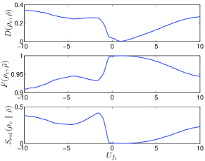
Figure 3: The distance $D$ and fidelity $F$ between $\rho_{c}$ and $\bar{\rho}$, and the relative entropy of $\rho_{c}$ with respect to $\bar{\rho}$, as functions of $U_{f_{1}}$. The initial state is the same as in Fig. 1.

III.2 Time evolution

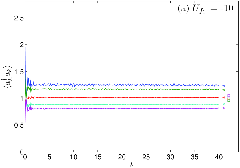
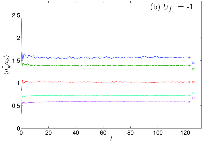
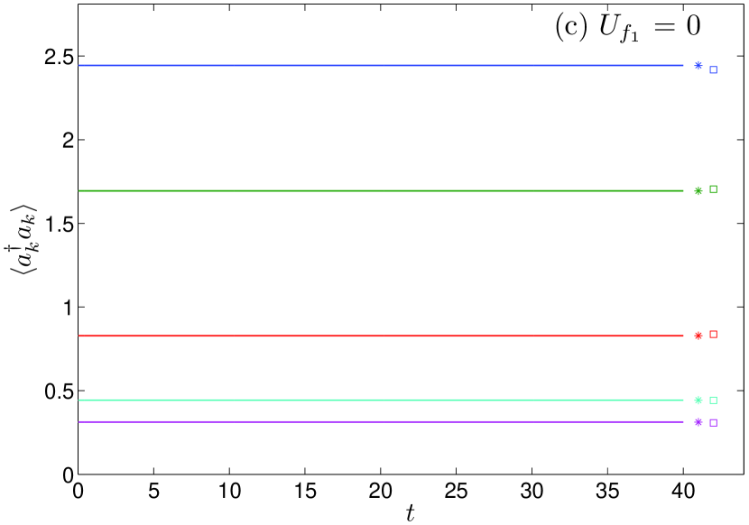
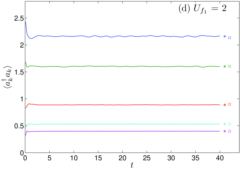
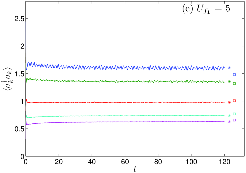
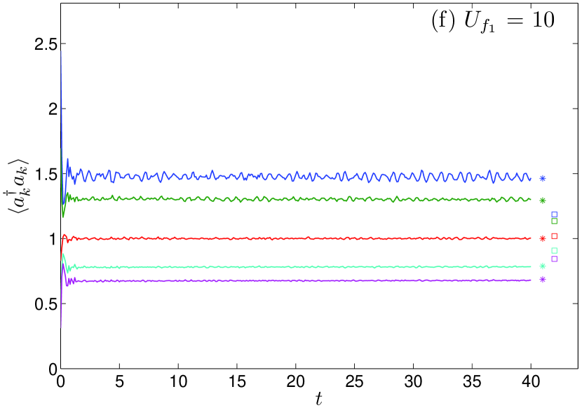
Figure 4: (Color online) Time evolution of the populations on the Bloch states $\langle a^{\dagger}_{k}a_{k}\rangle$. The figures correspond to those in Fig. 1 in a one-to-one manner. In each figure, from up to down, the five lines correspond to $k=0,\ldots,4$. Another $k$’s are now shown because $\langle a^{\dagger}_{k}a_{k}\rangle$ and $\langle a^{\dagger}_{M-k}a_{M-k}\rangle$ are close to each other all the time. For each line, the markers of the same color on the right hand side indicate the average value predicted by $\bar{\rho}$ ($*$) or value predicted by $\rho_{c}$ ($\square$), respectively. Note that in (b) and (e), the time span investigated is longer than that in others. This is because the transient times in (b) and (e) are relatively longer.

We now proceed to study the time evolution of the system after the quench. In Fig. 2, we show the time evolution of the populations on the Bloch states $\langle a^{\dagger}_{k}a_{k}\rangle$. The six sub-figures correspond to those in Fig. 1 respectively. For all the $U_{f_{1}}$’s and all the $k$’s, $\langle a_{k}^{\dagger}a_{k}\rangle$ equilibrate to their average values after a transient time, which is relatively longer in the cases of $U_{f_{1}}=-1$ and $5$. In the special case of $U_{f_{1}}=0$, there is no fluctuation at all. The reason is simply that in this case, $a^{\dagger}_{k}a_{k}$ are conserved. We see that the time-averaged values of $\langle a_{k}^{\dagger}a_{k}\rangle$ predicted by $\bar{\rho}$ ($*$) and $\rho_{c}$ ($\square$) agree relatively well in the cases of $U_{f_{1}}=0$ and $2$. This is consistent with the closeness between $\bar{\rho}$ and $\rho_{c}$ for these two values of $U_{f_{1}}$, as revealed in Fig. 1 and Fig. 3. Here we would say the system thermalizes well in the $U_{f_{1}}=2$ case, however, we would refrain making the same statement for the $U_{f_{1}}=0$ case. The reason will be clear in the next Section.

Figure 4 is about a finite-sized system with some specific initial condition. However, here we have some general statements. We argue that in the thermodynamic limit ($M,N\rightarrow\infty$ with $N/M$ fixed), as long as initially the system is at finite-temperature thermal equilibrium and described by a canonical ensemble density matrix as (2), we should see steady behaviors of the physical variables like $a^{\dagger}_{k}a_{k}$.

Let $A=a^{\dagger}_{k}a_{k}$ and let $A=\sum_{mn}A_{mn}|\psi^{f_{1}}_{m}\rangle\langle\psi^{f_{1}}_{n}|$ in the representation of $\{|\psi^{f_{1}}_{m}\rangle\}$. The ensemble-averaged value of $A$ at time $t$ is

$$a(t)=\sum_{mn}\rho_{mn}A_{nm}\exp[-i(E^{f_{1}}_{m}-E^{f_{1}}_{n})t],$$ (13)

where $\rho_{mn}\equiv\langle\psi^{f_{1}}_{m}|\rho_{i}|\psi^{f_{1}}_{n}\rangle$. Its time-averaged value is

$$\bar{a}=\lim_{T\rightarrow\infty}\frac{1}{T}\int_{0}^{T}dta(t)=\sum_{m}\rho_{mm}A_{mm}.$$ (14)

Here note that for a generic Hamiltonian $H_{f_{1}}$, there is no level degeneracy. The time-averaged value of $a^{2}(t)$ is peter

$$\overline{a^{2}} = \lim_{T\rightarrow\infty}\frac{1}{T}\int_{0}^{T}dta^{2}(t)$$ (15)

$$= \sum_{mp}\rho_{mm}A_{mm}\rho_{pp}A_{pp}+\sum_{m\neq n}\rho_{mn}A_{nm}\rho_{nm}A_{mn}$$

$$= \sum_{m}\rho_{mm}A_{mm}\sum_{p}\rho_{pp}A_{pp}+\sum_{m\neq n}|\rho_{mn}|^{2}|A_{mn}|^{2}$$

$$= \bar{a}^{2}+\sum_{m\neq n}|\rho_{mn}|^{2}|A_{mn}|^{2}.$$

Note that here it is assumed that there is no degeneracy of energy gaps. Thus we have for the variance of $a(t)$ in time, $\Delta^{2}a=\overline{a^{2}}-\bar{a}^{2}$,

$$\Delta^{2}a=\sum_{m\neq n}|\rho_{mn}|^{2}|A_{mn}|^{2}\leq\sum_{mn}|\rho_{mn}|^{2}|A_{mn}|^{2}.$$ (16)

Since $A$ is semi-positive definite and bounded, we have $|A_{mn}|^{2}\leq A_{mm}A_{nn}\leq N^{2}$. Thus we have

$$\Delta^{2}a\leq N^{2}\sum_{mn}|\rho_{mn}|^{2}.$$ (17)

Here we note that the summation is the square of the Frobenius norm of $\rho_{i}$ in the representation of $\{|\psi^{f_{1}}_{m}\rangle\}$, which is invariant in all representations and is preserved by an arbitrary unitary evolution horn . Explicitly, we have

$$\sum_{mn}|\rho_{mn}|^{2} = \sum_{mn}\langle\psi^{f_{1}}_{m}|\rho_{i}|\psi^{f_{1}}_{n}\rangle\langle\psi^{f_{1}}_{n}|\rho_{i}|\psi^{f_{1}}_{m}\rangle$$ (18)

$$= \sum_{m}\langle\psi^{f_{1}}_{m}|\rho_{i}^{2}|\psi^{f_{1}}_{m}\rangle=\sum_{m}\langle\psi^{i}_{m}|\rho_{i}^{2}|\psi^{i}_{m}\rangle$$

$$= \sum_{m}(p_{m}^{i})^{2}.$$

We argue that this quantity, which depends only on the initial state, decays exponentially with the size $M$. Let $E^{i}_{m}$ increase with $m$. We have

$$\sum_{m}(p_{m}^{i})^{2}<p_{1}^{i} = \frac{e^{-\beta_{i}E^{i}_{1}}}{Z_{i}}=\frac{e^{-\beta_{i}E^{i}_{1}}}{e^{-\beta_{i}F_{i}}}\simeq\frac{e^{-\beta_{i}\alpha M}}{e^{-\beta_{i}\gamma M}},\quad$$ (19)

as $M\rightarrow\infty$. Here in the $\simeq$ relation we used the fact the ground state energy $E^{i}_{1}$ of $H_{i}$ scales linearly with $M$ and so does the free energy $F_{i}$ of the initial state linear . The coefficients $\alpha$ and $\gamma$ are independent of $M$. Moreover, it is easy to see that $\alpha\geq\gamma$ for any $\beta_{i}$, with the equality taken only in the limit of $\beta_{i}=+\infty$ or $T_{i}=0^{+}$, and $\alpha-\gamma$ increases monotonically with $T_{i}$. This makes sure that $p_{1}^{i}$ would not grow exponentially with $M$ and transcend unity.

With (17) and (19), we get an upper bound for $\Delta a$,

$${\Delta a}\leq cM\exp(-\beta_{i}\theta M),\quad\theta=\frac{1}{2}(\alpha-\gamma)\geq 0,$$ (20)

where $c$ is some constant. The upper bound of $\Delta a$ helps us determine an upper bound for the probability of finding $a(t)$ deviating away from the mean $\bar{a}$ by a distance larger than $\epsilon$. Actually, following Reimann peter , using the Chebyshev inequality feller , we have

$$Prob(|a(t)-\bar{a}|>\epsilon)<\frac{\Delta^{2}a}{\epsilon^{2}}.$$ (21)

For a fixed value of $\epsilon$, the upper bound decreases exponentially with the size of the system according to (20). It then follows the statement above.

Here some comments are worthy. Though in the derivation above we have in mind a sudden quench, it is easy to see that the conclusion actually applies to any type of quench (e.g., the Hamiltonian can be changed continuously over some period, as in sengupta ; dimer , or quenched multiple times as in Sec. IV below), as long as after some point the Hamiltonian is never changed again. The reason lies in that the Frobenius norm of the density matrix $\rho(t)$ is conserved under unitary evolutions, and thus is independent of the historical or the final values of $H(t)$, but is determined entirely by the initial state. As for the operator $A$, only the properties of semi-positive-definiteness and boundedness are used. Thus similar conclusions can apply to other operators such as $a_{k}^{\dagger}a_{k}^{\dagger}a_{k}a_{k}$ and $a_{l}^{\dagger}a_{l}^{\dagger}a_{l}a_{l}$, or operators in other models. Finally, it should be mentioned that the conclusion relies on the fact that the quantity in Eq. (18) is bounded by some exponentially decreasing function, which is the case only at finite temperatures ($\beta_{i}<\infty$). At zero temperature, the quantity in Eq. (18) is always equal to unity and thus the problem is still open.

IV a second quench: typicality

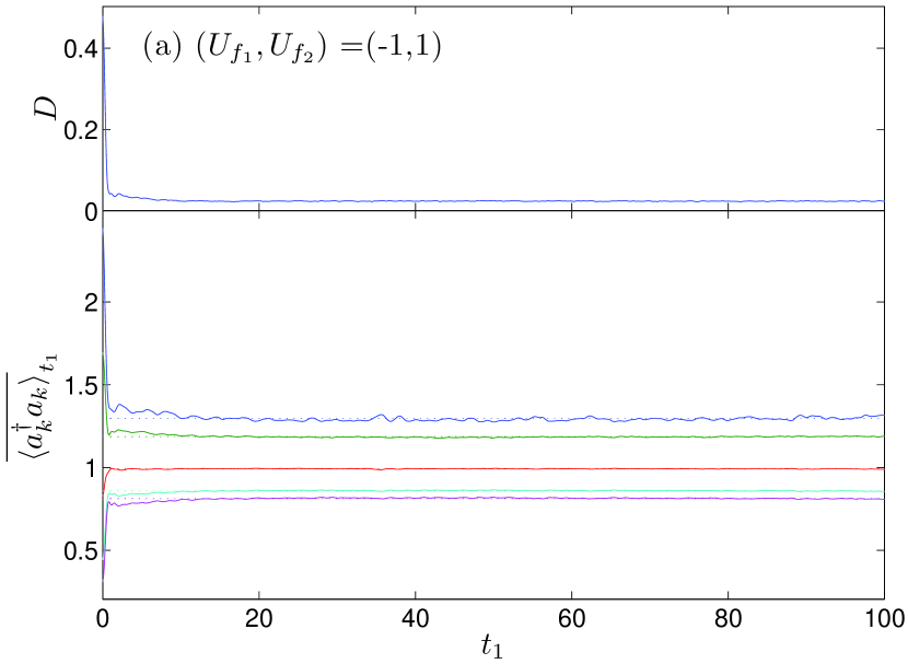
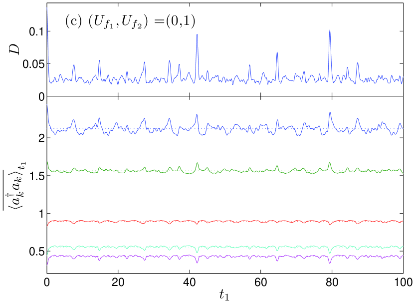
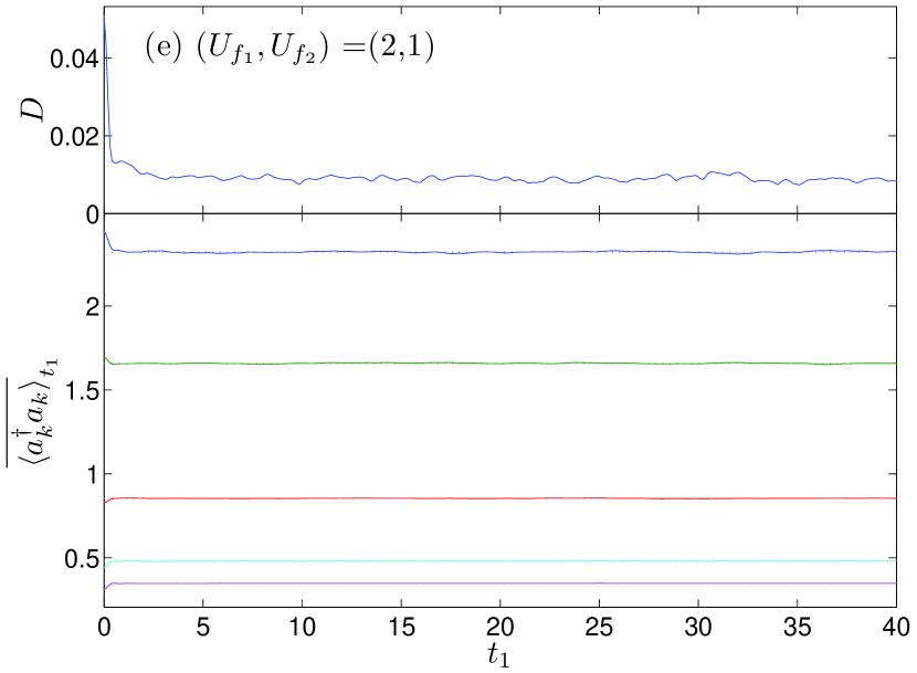
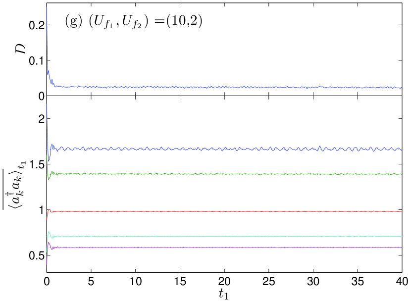
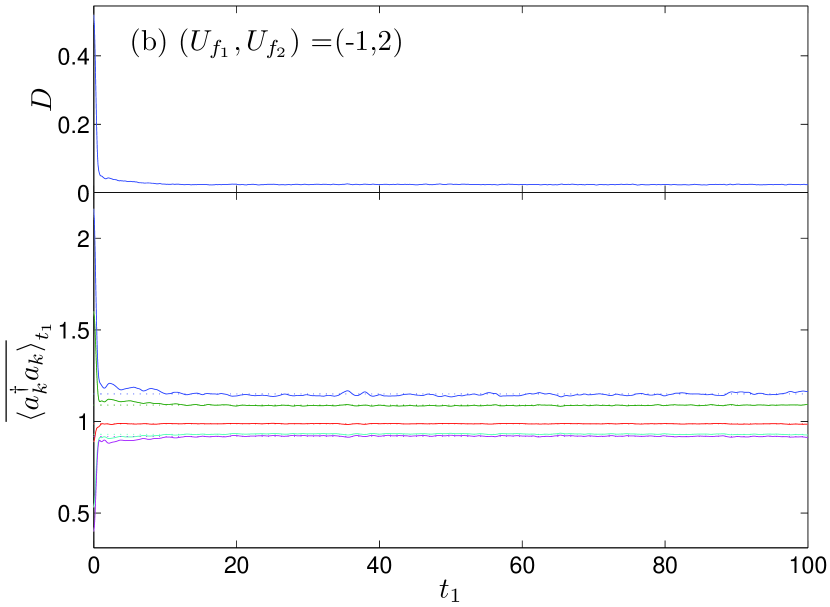
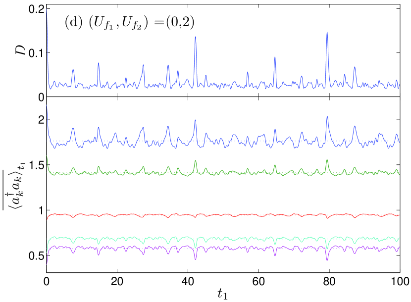
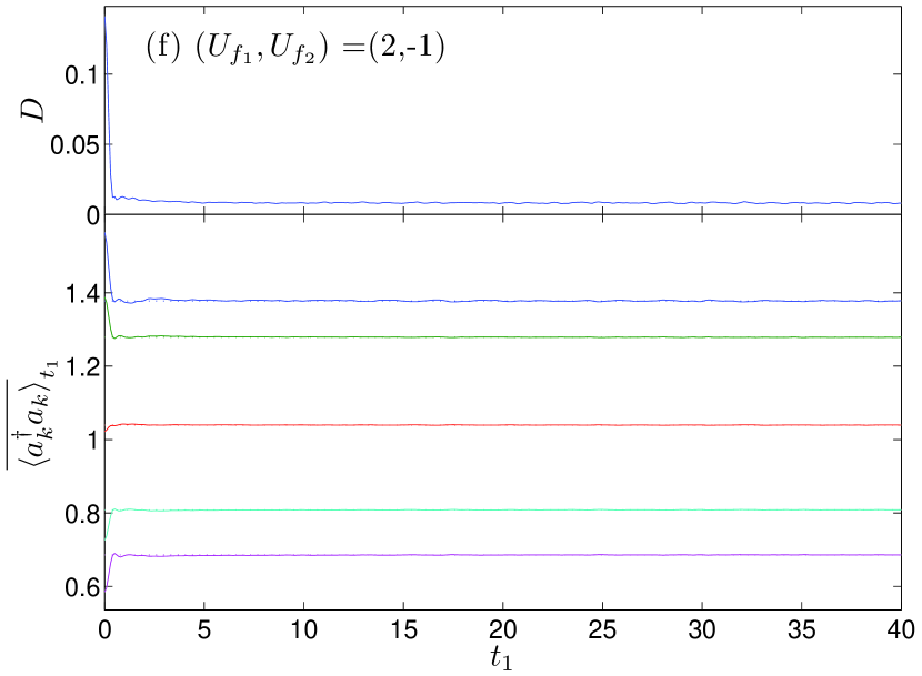
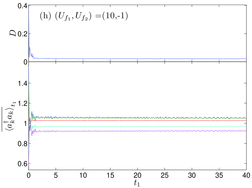
Figure 5: (Color online) The distance $D$ between the matrices $\Omega$ and $\bar{\rho}_{t_{1}}$ (upper panels) and the time-averaged values of $\langle a^{\dagger}_{k}a_{k}\rangle$ (lower panels), as functions of the time of the second quench $t_{1}$. The dashed lines in the lower panels indicate the average values of the corresponding solid lines, i.e., values given by $\Omega$ [see Eq. (25)]. The initial state is the same as in previous Figures. The parameters $(U_{f_{1}},U_{f_{2}})$ are shown in the inserts.

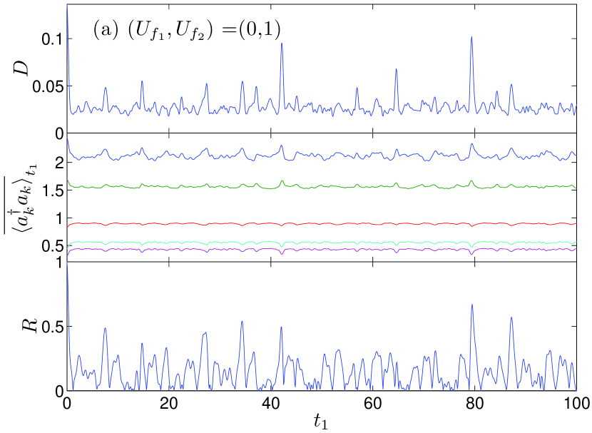
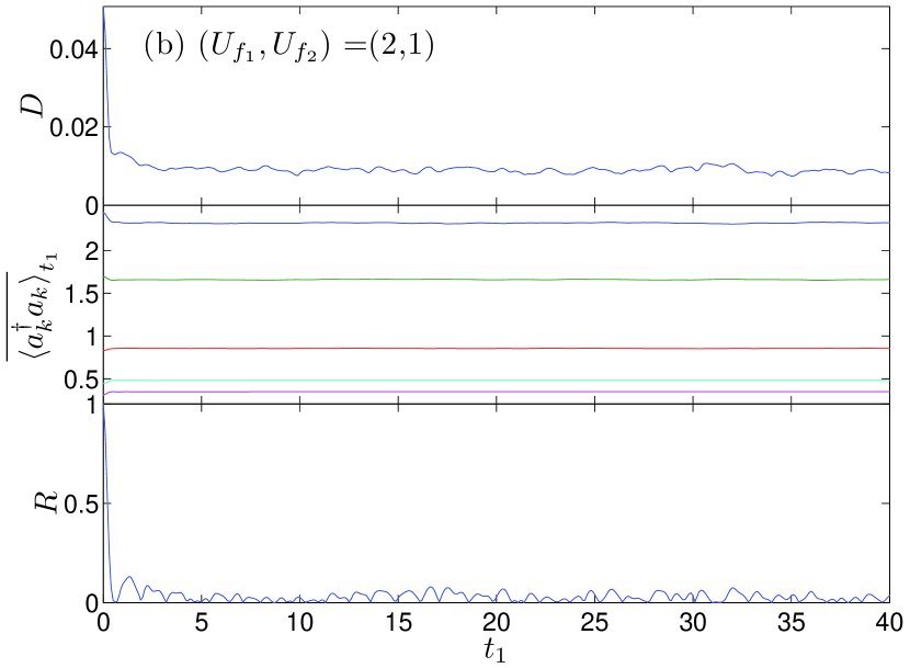
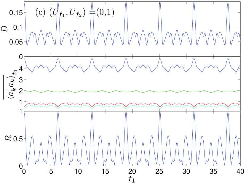
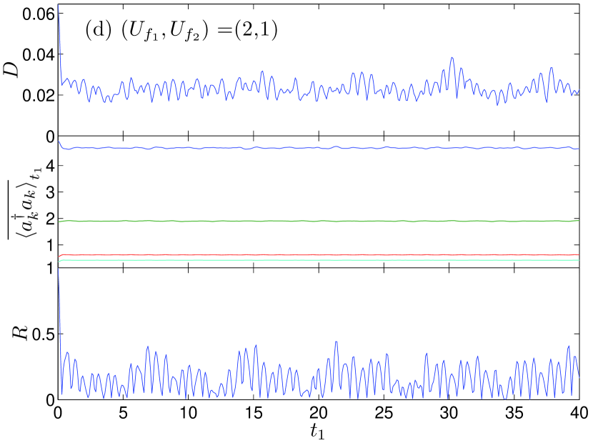
Figure 6: (Color online) The figure-of-merit of recurrence $R$ as a function of time. Also shown are $D(\Omega,\bar{\rho}_{t_{1}})$ and $\overline{\langle a^{\dagger}_{k}a_{k}\rangle}_{t_{1}}$. Note the correlation between the three in (a) and (c). In (a) and (b), the initial state is the same as in previous Figures, i.e., $(M,N,q,D_{q})=(9,9,1,2700)$, $U_{i}=1$, and $\beta_{i}=0.3$. In (c) and (d), the initial state is of $(M,N,q,D_{q})=(6,10,1,497)$, $U_{i}=1$, and $\beta_{i}=0.3$. The values of $(U_{f_{1}},U_{f_{2}})$ are given in the inserts.

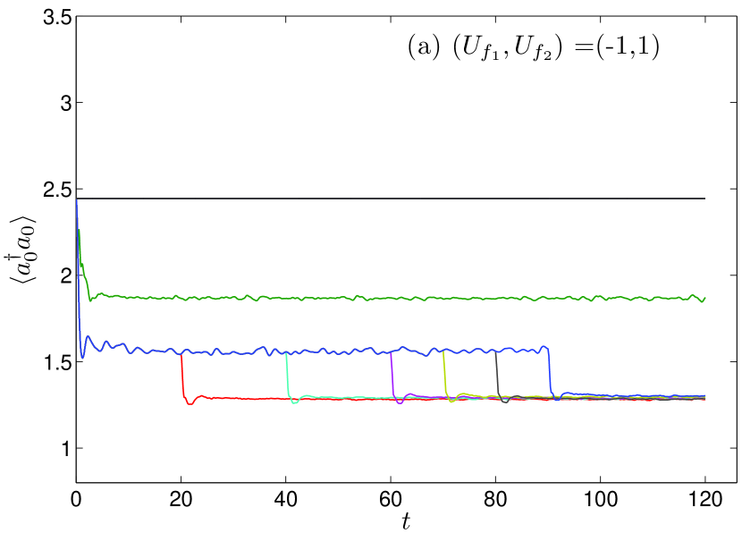
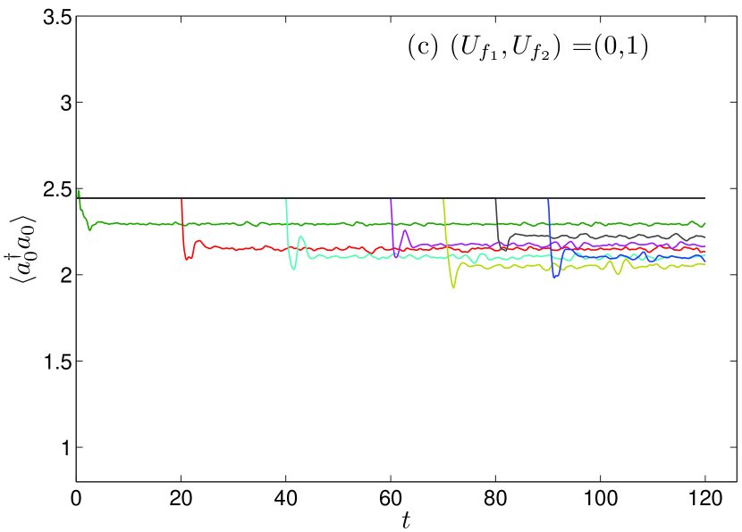
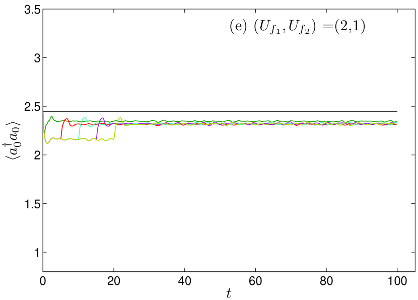
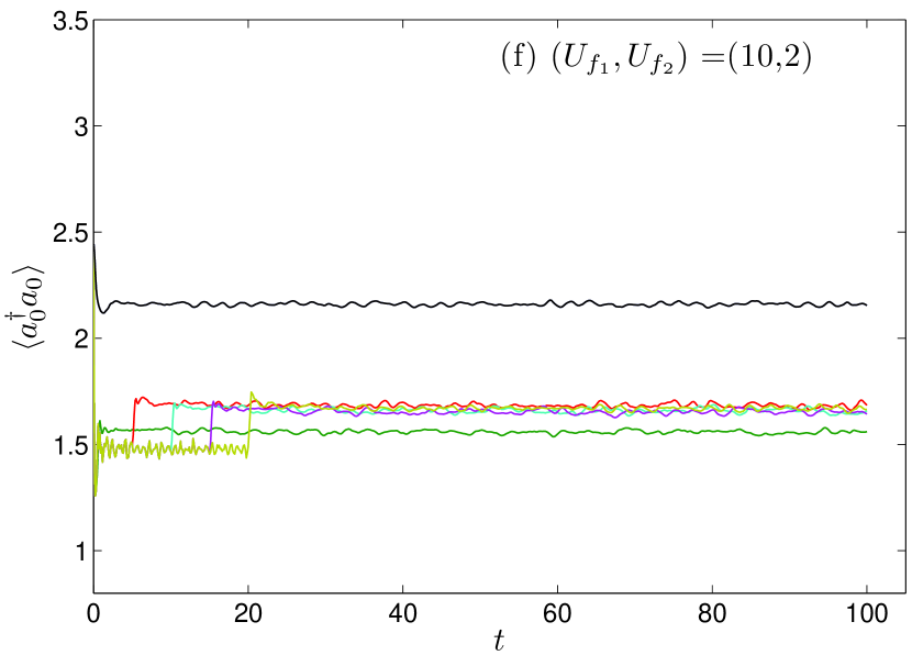
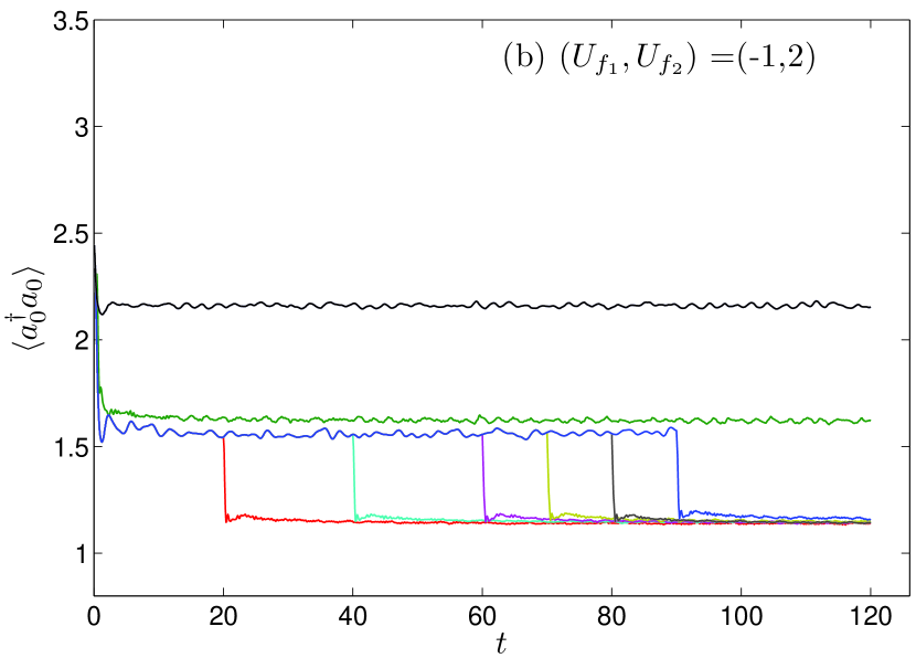
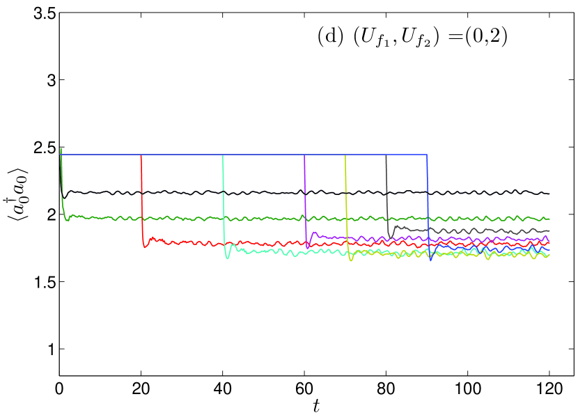
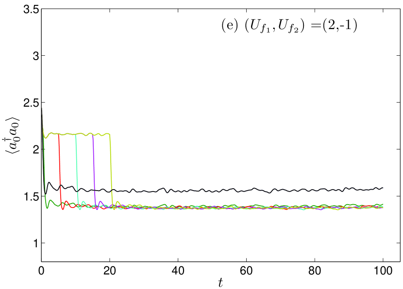
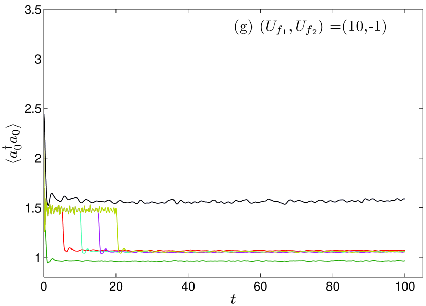
Figure 7: (Color online) Time evolution of the population on the $k=0$ Bloch state $\langle a_{0}^{\dagger}a_{0}\rangle$ test . Other $k$’s show similar behavior and thus are not shown. The figures correspond to those in Fig. 5 one-to-one. The initial state is the same as in Fig. 1 and Fig. 4. In (a)-(d), the different $t_{1}$’s investigated are $(0,0.35,20,40,60,70,80,90)$, while in (e)-(h), the different $t_{1}$’s are $(0,0.35,5,10,15,20)$. Note that in each figure, the black and green lines correspond to $t_{1}=0$ and $0.35$, respectively.

It is shown in Fig. 4 that after a finite transient time, the physical variables equilibrate to their average values exhibiting minimal fluctuations. Moreover, it has been proven that the amplitudes of the fluctuations will decrease exponentially with the size of the system. Therefore, the observation is that the system, described by the density matrix $\rho(t)$, is almost indistinguishable from a system described by the time-averaged density matrix $\bar{\rho}$, as far as the simple realistic physical variables are concerned. This is remarkable. Because though $\rho(t)$ evolves unitarily and suffers no loss of information of $\rho_{i}$, it behaves as if it were fully decoherenced. The question is then, to what extent can we hold onto this proposition? Is it possible to distinguish $\rho(t)$ and $\bar{\rho}$, or $\rho(t_{1})$ and $\rho(t_{2})$ ($t_{1}\neq t_{2}$), by some means? Motivated by this problem, we have considered the scenario of giving the quenched system a second quench. That is, after the first quench at $t=0$ which changes $U$ from $U_{i}$ to $U_{f_{1}}$, at time $t=t_{1}$, the system is quenched again by changing the value of $U$ from $U_{f_{1}}$ to $U_{f_{2}}$, which is then held on forever. The concern is, would the long-time dynamics of the system depends on the specific time $t_{1}$?

Denote the Hamiltonian associated with $U_{f_{2}}$ as $H_{f_{2}}$. The density matrix of the system later is given by $\rho(t)=e^{-iH_{f_{2}}(t-t_{1})}\rho(t_{1})e^{iH_{f_{2}}(t-t_{1})}$ (for $t>t_{1}$). As before, we are interested in the long-time averaged value of $\rho(t)$,

$$\bar{\rho}_{t_{1}}=\lim_{T\rightarrow\infty}\frac{1}{T}\int_{0}^{T}dt\rho(t_{1}+t),$$ (22)

since it has been shown and proven above that the dynamics of the system is to a large extent captured by the time-averaged density matrix. Here the subscript indicates the dependence on the time $t_{1}$. It is also useful to define the average of $\bar{\rho}_{t_{1}}$ with respect to $t_{1}$,

$$\Omega = \lim_{T\rightarrow\infty}\frac{1}{T}\int_{0}^{T}dt_{1}\bar{\rho}_{t_{1}}$$ (23)

$$= \lim_{T\rightarrow\infty}\frac{1}{T}\int_{0}^{T}dte^{-iH_{f_{2}}t}\bar{\rho}e^{iH_{f_{2}}t}.$$

The second equality means that $\Omega$ is actually the time-averaged density matrix associated with an initial state $\bar{\rho}$ [see Eqs. (4) and (5)] and a Hamiltonian $H_{f_{2}}$. One purpose of defining $\Omega$ is to set a reference state independent of $t_{1}$.

To gain an overall idea of the dependence on $t_{1}$ of the long-time dynamics, we have studied the distance between $\bar{\rho}_{t_{1}}$ and $\Omega$ chuang , and the time-averaged value of $\langle a_{k}^{\dagger}a_{k}\rangle$,

$$\overline{\langle a^{\dagger}_{k}a_{k}\rangle}_{t_{1}} \equiv \lim_{T\rightarrow\infty}\frac{1}{T}\int_{0}^{T}dt\cdot tr(\rho(t_{1}+t)a^{\dagger}_{k}a_{k})$$ (24)

$$= tr(\bar{\rho}_{t_{1}}a^{\dagger}_{k}a_{k}),$$

as functions of $t_{1}$. Note that the average value of $\overline{\langle a^{\dagger}_{k}a_{k}\rangle}_{t_{1}}$ with respect to $t_{1}$ is given by $\Omega$,

$$\lim_{T\rightarrow\infty}\frac{1}{T}\int_{0}^{T}dt_{1}\overline{\langle a^{\dagger}_{k}a_{k}\rangle}_{t_{1}}=tr(\Omega a^{\dagger}_{k}a_{k}).$$ (25)

This is another reason for defining $\Omega$. The quantities $D(\Omega,\bar{\rho}_{t_{1}})$ and $\overline{\langle a^{\dagger}_{k}a_{k}\rangle}_{t_{1}}$ are shown in Fig. 5. Eight pairs of $(U_{f_{1}},U_{f_{2}})$ are examined with the same initial condition as in Fig. 1. We see that for all cases with $U_{f_{1}}\neq 0$, both $D$ and $\overline{\langle a^{\dagger}_{k}a_{k}\rangle}_{t_{1}}$ set down to their average values quickly. However, for the special case of $U_{f_{1}}=0$, both $D$ and $\langle a_{k}^{\dagger}a_{k}\rangle_{t_{1}}$ display repeated recurrences, without any sign of equilibration. The situation is the reverse of that in Fig. 4, where $\langle a_{k}^{\dagger}a_{k}\rangle$ does not show any fluctuations in the case of $U_{f_{1}}=0$.

This phenomenon is due to the recurrence of the density matrix $\rho(t)$ to $\rho_{i}$ recur . From Eq. (3), we see that in the representation of $\{|\psi^{f_{1}}_{m}\rangle\}$, the $mn$-th off-diagonal element of $\rho(t)$ rotates at an angular frequency of $E^{f_{1}}_{m}-E^{f_{1}}_{n}$. In the generic case of $U_{f_{1}}\neq 0$, the energy gaps $E^{f_{1}}_{m}-E^{f_{1}}_{n}$ are quite random and incommensurate, and thus recurrence of the density matrix is rare. More precisely, the span between two times when all the matrix elements of $\rho(t)$ get (nearly) in phase again is extraordinarily large. On the contrary, in the special case of $U_{f_{1}}=0$, all eigenvalues and hence all the energy gaps $E^{f_{1}}_{m}-E^{f_{1}}_{n}$ are integral combinations of the few basic frequencies $\omega_{k}$, and thus the probability of recurrence is much higher. To demonstrate that the sharp peaks in Figs. 5c and 5d are due to recurrences of the density matrix $\rho(t)$ to $\rho_{i}$, we define the figure-of-merit of recurrence,

$$R(t)=\frac{|\sum_{m,n}^{\prime}\rho_{m,n}^{2}e^{-i(E^{f_{1}}_{m}-E^{f_{1}}_{n})t}|}{\sum_{m,n}^{\prime}\rho_{mn}^{2}},$$ (26)

where the prime means the summation is over $(m,n)$ such that $E^{f_{1}}_{m}\neq E^{f_{1}}_{n}$. It is clear that $0\leq R\leq 1$ and $R=1$ when and only when all the off-diagonal elements get in phase.

In Figs. 6a and 6b, which share the same parameters as Figs. 5c and 5e respectively, we have shown $R(t_{1})$ together with $D(\Omega,\bar{\rho}_{t_{1}})$ and $\overline{\langle a^{\dagger}_{k}a_{k}\rangle}_{t_{1}}$. In Fig. 6a, we see that every time $D(\Omega,\bar{\rho}_{t_{1}})$ and $\overline{\langle a^{\dagger}_{k}a_{k}\rangle}_{t_{1}}$ get close to their values at $t_{1}=0$, $R(t_{1})$ shows a peak. In other words, there is a strong positive correlation between $R(t_{1})$ and $D(\Omega,\bar{\rho}_{t_{1}})$ and $\overline{\langle a^{\dagger}_{k}a_{k}\rangle}_{t_{1}}$. In comparison, in Fig. 6b, $R(t_{1})$ drops quickly from unity to less than $0.2$ and remains low all the time, and in turn $D(\Omega,\bar{\rho}_{t_{1}})$ and $\overline{\langle a^{\dagger}_{k}a_{k}\rangle}_{t_{1}}$ do not show any recurrence. To further consolidate the connection between the recurrence of $\rho(t)$ and that of $D(\Omega,\bar{\rho}_{t_{1}})$ and $\overline{\langle a^{\dagger}_{k}a_{k}\rangle}_{t_{1}}$, we have considered the case of $M=6$. In this case, if $U_{f_{1}}=0$, all the basic frequencies $\omega_{k}$ are commensurate, and thus there exist perfect recurrences, as shown in Fig. 6c. There we see clearly that $D(\Omega,\bar{\rho}_{t_{1}})$ and $\overline{\langle a^{\dagger}_{k}a_{k}\rangle}_{t_{1}}$ return to their original values at $t_{1}=0$ periodically, and this happens when and only when $R$ returns to unity. However, once $U_{f_{1}}\neq 0$ is set nonzero (see Fig. 6d) and thus the commensurability of the energy gaps is destroyed, the situation returns to that in Fig. 6b.

The fact revealed in Fig. 5 and Fig. 6 is quite interesting. The long-time dynamics of the system is sensitive or insensitive to the exact time when the second quench is applied, depending on whether the intermediate Hamiltonian $H_{f_{1}}$ is integrable ($U_{f_{1}}=0$) or non-integrable ($U_{f_{1}}\neq 0$). In the integrable case, $\overline{\langle a^{\dagger}_{k}a_{k}\rangle}_{t_{1}}$ exhibits large fluctuations and repeated recurrences. The system retains the memory of the initial state under the control of the Hamiltonian $H_{f_{1}}$. By contrast, in the non-integrable case, $\overline{\langle a^{\dagger}_{k}a_{k}\rangle}_{t_{1}}$ go over to their average values (predicted by $\Omega$) after a transitory period, showing little dependence on $t_{1}$ afterwards. Combined with Fig. 4, the picture is that $\rho(t)$ evolving under the control of a non-integrable Hamiltonian, not only yields the expectation values of $a_{k}^{\dagger}a_{k}$ as if it were $\bar{\rho}$, but even responds to the second quench as if it were $\bar{\rho}$.

In Fig. 7, we have checked this picture by studying the real time evolution of $\langle a_{k}^{\dagger}a_{k}\rangle$ with $k=0$ under the double-quench scenario. The eight figures shown correspond to those in Fig. 5 respectively. For each pair of $(U_{f_{1}},U_{f_{2}})$, we have studied the evolution of $\langle a_{0}^{\dagger}a_{0}\rangle$ for several different values of $t_{1}$. We see that in all the cases with $U_{f_{1}}\neq 0$, as long as $t_{1}$ is larger than the transient time, which can be roughly read from Fig. 5, the later evolution of $\langle a_{0}^{\dagger}a_{0}\rangle$ is quantitatively independent of $t_{1}$. On the contrary, in the case with $U_{f_{1}}=0$, the later values of $\langle a_{0}^{\dagger}a_{0}\rangle$ vary wildly for different values of $t_{1}$.

Here it is instructive to combine Fig. 4 and Fig. 7 and compare. In the $U_{f_{1}}\neq 0$ cases, there is a sense of typicality goldstein ; popescu . The density matrix $\rho(t)$ governed by $H_{f_{1}}$ is surely non-stationary. However, for $\rho(t)$ at different times, they yield almost the same expectation values for the observables, and moreover, they share almost the same response to the same quench. In the case of $U_{f_{1}}=0$, what Fig. 7 reveals is a good complement to that in Fig. 4. It demonstrates that it is inappropriate to say that the system thermalizes in this case, even though the density matrices and expectation values of the observables agree—since according to one’s everyday experience, a system in thermal equilibrium should not show any time dependence.

V conclusions and discussions

We have studied the quench dynamics of the Bose-Hubbard model both analytically and numerically. The issues of thermalization and equilibration are investigated thoroughly.

On the thermalization side, which concerns whether the quenched system behaves like a canonical ensemble, it is found that this is the case only for small-amplitude quenches (at least for the finite-sized system investigated). However, the time-averaged density matrix does manifest many interesting features in different regimes. These features are self-consistently understood after a study of the overlaps between the eigenstates of $H_{i}$ and $H_{f_{1}}$. Here we would like to say that it is urgent and would be very helpful to develop some analytical tools so that some general relations between the eigen-systems of $H_{i}$ and $H_{f_{1}}$ can be established. These tools and relations would also be useful to determine whether the non-thermalization phenomenon observed is just a finite-size effect.

On the equilibration side, which is about whether physical observables relax to stationary values without appreciable fluctuations, the result is that this is indeed the case for quantities as $\langle a^{\dagger}_{k}a_{k}\rangle$ which are of most interest. Moreover, it is proven analytically that for these quantities the fluctuations in time will decay exponentially with the size of the system. Therefore, the overall picture is that generally the system equilibrates but without thermalization.

The second quench reveals something more subtle. First, the subsequent dynamics depends or not on the second quench time $t_{1}$ according to $U_{f_{1}}=0$ or not. The underline reason is the recurrence or not of the initial density matrix, which in turn has its root in the eigenvalue statistics of the Hamiltonian $H_{f_{1}}$. This effect leaves us the impression that a non-integrable Hamiltonian has more “dephasing power” than an integrable one. Possibly it can be a tool to check the integrability of a Hamiltonian. Second, in the case of $U_{f_{1}}\neq 0$, it is found that the system described by $\rho(t_{1})$ responds to the second quench as if it were $\bar{\rho}$ for $t_{1}$ larger than the transient time. This means that we can take the equilibration more serious—$\rho(t_{1})$ and $\bar{\rho}$ not only yield almost the same expectation values for the generic physical variables but also yield almost the same dynamics after a quench. Moreover, the fact that the transient time is short indicates that the intermediate Hamiltonian $H_{f_{1}}$, which is non-integrable, is effective in “dephasing” the initial density matrix. In another perspective, the dynamics of the system is sensitive to the fluctuations of $U$. This has the implication that in future experiments, accurate control of $U$ would be a necessity to interpret the results correctly.

VI acknowledgment

We are grateful to H. T. Yang, Z. X. Gong, Y.-H. Chan, L. M. Duan, and D. L. Zhou for stimulating discussions and valuable suggestions. J. M. Z. is supported by NSF of China under Grant No. 11091240226.

References

- (1) S. Trotzky, Y.-A. Chen, A. Flesch, I. P. McCulloch, U. Schollwc̈k, J. Eisert, and I. Bloch, arXiv:1101.2659.
- (2) T. Kinoshita, T. Wenger, and D. S. Weiss, Nature (London) 440, 900 (2006).
- (3) G. Roux, Phys. Rev. A 81, 053604 (2010).
- (4) G. Roux, Phys. Rev. A 79, 021608(R) (2009).
- (5) C. Kollath, A. M. Lauchli, and E. Altman, Phys. Rev. Lett. 98, 180601 (2007).
- (6) M. Rigol, V. Dunjko, V. Yurovsky, and M. Olshanii, Phys. Rev. Lett. 98, 050405 (2007).
- (7) S. R. Manmana, S. Wessel, R. M. Noack, and A. Muramatsu, Phys. Rev. Lett. 98, 210405 (2007).
- (8) M. Rigol, Phys. Rev. Lett. 103, 100403 (2009).
- (9) M. Rigol, V. Dunjko, and M. Olshanii, Nature (London) 452, 854 (2008).
- (10) A. V. Ponomarev, S. Denisov, and P. Hänggi, Phys. Rev. Lett. 106, 010405 (2011).
- (11) M. Greiner, O. Mandel, T. W. Hänsch, and I. Bloch, Nature (London) 419, 51 (2002).
- (12) M. A. Cazalilla, Phys. Rev. Lett. 97, 156403 (2006).
- (13) C. Trefzger and K. Sengupta, arXiv:1008.1285.
- (14) T. Venumadhav, M. Haque, and R. Moessner, Phys. Rev. B 81, 054305 (2010).
- (15) C. De Grandi, V. Gritsev, and A. Polkovnikov, Phys. Rev. B 81, 012303 (2010).
- (16) D. Jaksch, C. Bruder, J. I. Cirac, C. W. Gardiner, and P. Zoller, Phys. Rev. Lett. 81, 3108 (1998).
- (17) M. Greiner, O. Mandel, T. Esslinger, T. W. Hänsch, and I. Bloch, Nature (London) 415, 39 (2002).
- (18) I. Bloch, Nat. Phys. 1, 23 (2005).
- (19) R. B. Diener, Q. Zhou, H. Zhai, and T.-L. Ho, Phys. Rev. Lett. 98, 180404 (2007).
- (20) Y. Kato, Q. Zhou, N. Kawashima, and N. Trivedi, Nat. Phys. 4, 617 (2008).
- (21) N. Linden, S. Popescu, A. J. Short, and A. Winter, Phys. Rev. E 79, 061103 (2009).
- (22) I. Bloch, J. Dalibard, and W. Zwerger, Rev. Mod. Phys. 80, 885 (2008).
- (23) J. M. Zhang, C. Shen, and W. M. Liu, arXiv:1102.2469.
- (24) J. M. Zhang and R. X. Dong, Eur. J. Phys. 31, 591 (2010).
- (25) For example, the fitting parameter varies little among the -subspaces.
- (26) We note that the Bose-Hubbard model with a negative has not a well-defined thermodynamic limit. However, this should not prevent us from studying the negative- case at finite sizes.
- (27) It is so called because and .
- (28) M. A. Nielsen and I. L. Chuang, Quantum Computation and Quantum Information (Cambridge University Press, 2000).
- (29) P. Reimann, Phys. Rev. Lett. 101, 190403 (2008).
- (30) R. A. Horn and C. R. Johnson, Matrix Analysis (Cambridge University Press, New York, 1985), p. 291.
- (31) This is surely not the case for . But it is believed that it is indeed the case for .
- (32) W. Feller, An Introduction to Probability Theory and Its Applications I (Wiley, New York, 1968).
- (33) P. Bocchieri and A. Loinger, Phys. Rev. 107, 337 (1957); I. C. Percival, J. Math. Phys. 2, 235 (1961).
- (34) Only the quantity is shown because it constitutes the most strigent test.
- (35) S. Goldstein, J. L. Lebowitz, R. Tumulka, and N. Zanghi, Phys. Rev. Lett. 96, 050403 (2006).
- (36) S. Popescu, A. J. Short, and A. Winter, Nat. Phys. 2, 754 (2006).