Saddles, Arrows, and Spirals: Deterministic Trajectories in Cyclic Competition of Four Species

Abstract

Population dynamics in systems composed of cyclically competing species has been of increasing interest recently. Here, we investigate a system with four or more species. Using mean field theory, we study in detail the trajectories in configuration space of the population fractions. We discover a variety of orbits, shaped like saddles, spirals, and straight lines. Many of their properties are found explicitly. Most remarkably, we identify a collective variable which evolves simply as an exponential: $\mathcal{Q}\propto e^{\lambda t}$, where $\lambda$ is a function of the reaction rates. It provides information on the state of the system for late times (as well as for $t\rightarrow-\infty$). We discuss implications of these results for the evolution of a finite, stochastic system. A generalization to an arbitrary number of cyclically competing species yields valuable insights into universal properties of such systems.

I Introduction

In the study of population dynamics for biological systems or chemical reactions, it is customary to start with a set of ordinary differential/difference equations which model the time evolution of populations or concentrations. These would be appropriate if the various constituents of the system are well mixed (so that spatial structures can be ignored) and if the stochastic aspects of the evolution can be overlooked. In this sense, the term ‘mean field theory’ (MFT) is most appropriate, as both spatial and temporal fluctuations are absent. Despite these limitations, MFT has proven valuable in several respects. As in other areas of statistical physics, it typically provides an adequate description in much of the space of (control) parameters, e.g., Landau’s theory of phase transitions. In addition, it yields significant insights into many interesting phenomena associated with the underlying non-linear dynamics. A well known example is the simple logistic map, which gives rise to a rich structure of bifurcation, chaos, and universality May76 ; Feig78 ; Feig79 . Finally, it provides a stage on which hidden symmetries can be showcased readily.

In this context, we are motivated to consider MFT for a simple model of population dynamics, involving four species competing cyclically. This is a generalization of systems with three cyclically competing species, also known as the rock-paper-scissors games, which attracted considerable attention in recent years Fra96a ; Fra96b ; Pro99 ; Tse01 ; Ker02 ; Kir04 ; Rei06 ; Rei07 ; Rei08 ; Cla08 ; Pel08 ; Rei08a ; Ber09 ; Ven10 ; Shi10 ; And10 ; Rul10 ; Wan10 ; Mob10 ; He10 ; Win10 ; Dob10 . Labeling the species $a,b,c,d$, we allow $a$ to ‘prey on’ $b$ with some rate, and $b,c,d$ to ‘prey on’ $c,d,a$, respectively, with some other rates. Unlike earlier studies, we will not restrict our rates, but consider them in general. As we will show, apart from having a much larger and complex parameter space, the four species system (4SS) is qualitatively different. Indeed, in MFT, the evolution of the three species system (3SS) is relatively trivial, since a non-linear invariant (a hidden symmetry) renders all trajectories into closed orbits on a plane. As a result, there is little hint of the presence of absorbing states, which are of fundamental interest for the study of extinction probabilities in a stochastic system. By contrast, such a scenario is not the case, typically, for the 4SS. In addition, when one species becomes extinct, our problem reduces to an apparently trivial limit of the 3SS. Yet, the MFT offers useful and quantitative predictions. In a separate publication CDPZ-JSTAT , we will present extensive simulations of the full stochastic model and show that many of the MFT predictions are well born out. In this article, we will focus only on the deterministic MFT and the rich variety of phenomena it predicts. Though some of the preliminary results on the 4SS have been presented earlier CDPZ-epl , this paper will delve into not only details of the analysis, but also provide new insights into the behavior of systems with $S>4$ species.

Before we begin, we should mention that there are studies for the general $S$ case, though far few in number than for the 3SS. Most of these studies considered systems on one- or two-dimensional lattices Fra96a ; Fra96b ; Fra98 ; Kob97 ; Sat02 ; Sza04 ; He05 ; Sza07b ; Sza08 ; Dob10 . Due to the presence of spatial structure, these systems display far more complex behavior and so, the authors typically restrict themselves to special sets of rates (e.g., all equal, or all but one being equal). Finally, some studies, motivated by real-world systems, focused on a large number of competing species with more complicated interactions schemes Sil92 ; Sza01 . Here, we will focus on phenomena that emerge from arbitrary (positive) rates, but consider only systems with no spatial structure. An interesting application of a four-species model without spatial structure to the endogenous and exogenous origins of diseases can be found in Sor09 .

This paper is organized as follows. Though our main focus will be MFT, we will first discuss how the differential equations arise from a fully stochastic, microscopic model of the 4SS. Details of the latter (which can be simulated by Monte Carlo methods) and the associated master equation will be presented in Section II. The approximation scheme which leads to the MFT will also be provided. Section III will be devoted to the analysis of the MFT equations, with a number of explicit results. Their implications for the stochastic evolution will be considered in Section IV. By generalizing to systems with $S>4$ cyclically competing species, we gain deeper insights into how certain aspects of the solutions are ‘universal.’ These considerations will be presented in Section V. Readers who are comfortable with abstract formulations will find that some of the conclusions in Sections III are just special cases. Finally, we will summarize our findings in a concluding section and sketch possible avenues for future research.

Interestingly, we found CDPZ-epl that, unlike in the 3SS, the four species form partner-pairs, much like in the game of Bridge. In a system with $N$ individuals, there are $2\left(N+1\right)$ absorbing states, most of which consist of a surviving partner-pair. Since MFT is best suited for systems with large $N$, we should expect that all the final states in this approximation to consists of a coexisting pair: either $a$-$c$ or $b$-$d$. Of course, many interesting issues associated with the full, stochastic model (e.g., extinction probabilities) cannot be answered by MFT, while simulations reveal complex extinction scenarios that depend on both the predation rates and initial conditions. Since those investigations are quite extensive, they will be reported elsewhere CDPZ-JSTAT .

II The microscopic stochastic model and its mean field approximation

Our four species system consists of $N_{m}$ individuals of species $m=\left(a,b,c,d\right)$. With no spatial structure, any individual can interact with any other, in a cyclically competing manner. In a time step of a fully stochastic model, a random pair is chosen and, if they are ‘cyclically different,’ the following interactions occur with probabilities $p_{m}:$

$$a+b\stackrel{{\scriptstyle p_{a}}}{{\rightarrow}}a+a;\,\,b+c\stackrel{{\scriptstyle p_{b}}}{{\rightarrow}}b+b$$

$$c+d\stackrel{{\scriptstyle p_{c}}}{{\rightarrow}}c+c;\,\,d+a\stackrel{{\scriptstyle p_{d}}}{{\rightarrow}}d+d$$

Thus, the total number in the system

$$N=\sum_{m}N_{m}$$

is a constant and the full configuration space is just a set of points within a regular tetrahedron (of length $N$ on each side, with the four vertices being $N=N_{m}$ for one of the $m$’s). Of course, we will later consider the fractions $N_{m}/N$, which are natural variables in the large $N$ limit and the mean field approximation.

Let us emphasize that $ac$ and $bd$ pairs do not interact, so that it is possible for the final (absorbing) state to display coexistence of these pairs. In other words, any point along the $a$-$c$ and $b$-$d$ edges of the tetrahedron represents such a state. Indeed, this property provides the first major difference between our 4SS and the simpler 3SS: We have $2\left(N+1\right)$ absorbing states here instead of just $3$ (regardless of $N$). We should also remark that each face of the tetrahedron is also ‘absorbing’ in the sense that transitions into the face are irreversible. Within each face, the problem is a special limit of the 3SS, namely, one of the three rates being zero.

Given the interaction rules, the master equation for $P\left(\left\{N_{m}\right\};\tau\right)$, the probability for finding the system $\tau$ steps after a particular initial distribution $P_{0}\left(\left\{N_{m}\right\}\right)$, can be easily written. It provides the change in $P$ over one step:

$$P\left(\left\{N_{m}\right\};\tau+1\right)-P\left(\left\{N_{m}\right\};\tau\right)$$ (1)

$$= \frac{p_{a}\left(N_{a}-1\right)\left(N_{b}+1\right)}{N\left(N-1\right)/2}P\left(N_{a}-1,N_{b}+1,N_{c},N_{d};\tau\right)$$

$$+\frac{p_{b}\left(N_{b}-1\right)\left(N_{c}+1\right)}{N\left(N-1\right)/2}P\left(N_{a},N_{b}-1,N_{c}+1,N_{d};\tau\right)$$

$$+\frac{p_{c}\left(N_{c}-1\right)\left(N_{d}+1\right)}{N\left(N-1\right)/2}P\left(N_{a},N_{b},N_{c}-1,N_{d}+1;\tau\right)$$

$$+\frac{p_{d}\left(N_{d}-1\right)\left(N_{a}+1\right)}{N\left(N-1\right)/2}P\left(N_{a}+1,N_{b},N_{c},N_{d}-1;\tau\right)$$

$$-\frac{Z}{N\left(N-1\right)/2}P\left(\left\{N_{m}\right\};\tau\right)$$

where

$$Z\equiv p_{a}N_{a}N_{b}+p_{b}N_{b}N_{c}+p_{c}N_{c}N_{d}+p_{d}N_{d}N_{a}\,\,.$$ (2)

For the initial $P_{0}\left(\left\{N_{m}\right\}\right)$, it is sufficient to use $\delta$ distributions. Indeed, every simulation run begins with a single point (e.g., the symmetry point $N_{m}=N/4$)! Since the master equation is linear, the evolution starting with any other distribution is just the sum of the $P$’s that begin as $\delta$’s at various appropriate points.

From the master equation for $P\left(\left\{N_{m}\right\};\tau\right)$, we can easily derive a partial differential equation for the associated generating function. But, to find the solution for either equation is far from trivial. Instead, we turn to the mean field approximation, which should be adequate for large $\left\{N_{m}\right\}$. Thus, we can expect break downs near the extinction of one or more species, i.e., near an ‘absorbing face’ or an absorbing state.

In a MFT, the focus is the evolution of the averages of say, the fractions $N_{m}/N$, denoted by

$$A\left(\tau\right) \equiv \left\langle N_{a}/N\right\rangle_{\tau}\equiv\sum_{\left\{N_{m}\right\}}\left(N_{a}/N\right)P\left(\left\{N_{m}\right\};\tau\right)\,\,,$$

$$B\left(\tau\right) \equiv \left\langle N_{b}/N\right\rangle_{\tau},\,C\left(\tau\right)\equiv\left\langle N_{c}/N\right\rangle_{\tau},\,D\left(\tau\right)\equiv\left\langle N_{d}/N\right\rangle_{\tau}$$

Of course, we have the constraint

$$A+B+C+D=1$$ (3)

so that there are only three independent variables.

Following standard routes, we can derive an equation for the changes, $A\left(\tau+1\right)-A\left(\tau\right)$, etc., from the master equation (1). These will involve averages of products (e.g., $\left\langle N_{a}N_{b}\right\rangle_{\tau}$) on the right. The mean field approximation consists of neglecting all correlations and replacing the averages of products by the products of averages, so that the end result is a closed set of deterministic equations for $A\left(\tau\right)$, $B\left(\tau\right)$, etc. Finally, by taking the $N\rightarrow\infty$ limit, defining $t\equiv\tau/N$ (which can be regarded as continuous), and letting $A\left(\tau+1\right)-A\left(\tau\right)\rightarrow\left(1/N\right)\partial_{t}A\left(t\right)$, we arrive at the MFT equations:

$$\partial_{t}A = \left[k_{a}B-k_{d}D\right]A$$ (4)

$$\partial_{t}B = \left[k_{b}C-k_{a}A\right]B$$ (5)

$$\partial_{t}C = \left[k_{c}D-k_{b}B\right]C$$ (6)

$$\partial_{t}D = \left[k_{d}A-k_{c}C\right]D$$ (7)

In these time units, the ‘rates’ $k_{m}$ can be related to the original probabilities via $k_{m}=2p_{m}$. In the literature, however, time is often rescaled again, so as to normalize the rates to

$$k_{a}+k_{b}+k_{c}+k_{d}=1$$ (8)

as well.

III Analysis of MFT equations

This section will be devoted to the implications of eqns. (4-7), assuming the initial fractions are $\left(A_{0},B_{0},C_{0},D_{0}\right)$. Given the normalization (8), our parameter space is, in general, quite large: 6-dimensional. We will begin with a restricted problem – evolution on one of the faces of the tetrahedron – which is explicitly solvable.

III.1 Evolution when one species is extinct

Clearly, this restricted problem is not only much simpler than the full 4SS, it is also considerably simpler than the general 3SS. The reason is obvious: One of the three remaining species does not ‘consume’ anyone and so, its numbers can never increase. Without loss of generality, let us consider the face with $D=0$ with arbitrary initial $\left(A_{0},B_{0},C_{0}\right)$. In this case, neither $k_{c}$ nor $k_{d}$ plays a role, while eqns. (4-7) reduce significantly. As a result,

$$R\equiv A^{k_{b}}C^{k_{a}}$$ (9)

is an invariant (similar to that in the full 3SS Ber09 ), so that it is always fixed at $A_{0}^{k_{b}}C_{0}^{k_{a}}$. Of course, our problem now reduces to one with a single variable, which we choose to be

$$V\equiv A^{k_{b}}C^{-k_{a}}$$ (10)

so that its evolution is monotonically increasing until $B$ vanishes:

$$\partial_{t}\ln V=2k_{a}k_{b}B\geq 0$$ (11)

Meanwhile, $B=1-A-C$ and $A^{2k_{b}}$ ($C^{2k_{a}}$) is given by $RV$ ($R/V$), so that the full solution for $V\left(t\right)$ can be obtained through the integral

$$\int_{V_{0}}^{V\left(t\right)}\frac{dv}{v\left[1-\left(Rv\right)^{1/2k_{b}}-\left(R/v\right)^{1/2k_{a}}\right]}=2k_{a}k_{b}t$$ (12)

where $V_{0}\equiv A_{0}^{k_{b}}C_{0}^{-k_{a}}$. Though analytically precise, this form of the solution does not provide much insight on the evolution of the system. Instead, a schematic plot of sample trajectories, as shown in Fig. 1, should be much more helpful. Representing various values of $R$, the curved lines (dashed, red online) are generalized hyperbolas (9). The initial fractions $\left(A_{0},B_{0},C_{0}\right)$ dictate which curve that system will follow, while the evolution takes it towards larger $A$ (in the direction of the arrows, blue online), ending at a point $\left(A_{f},0,C_{f}\right)$ on the $a$-$c$ line. Note that the straight line (dot-dashed, green online), given by $k_{b}C=k_{a}A$, intersects each of these curves at right angles, corresponding to $B$ being maximal at these points. Finally, by exploiting the invariant $R$, the values $A_{f}$ and $C_{f}$ ($=1-A_{f}$) can be found from a (generally transcendental) equation, e.g.,

$$A_{f}^{k_{b}}\left(1-A_{f}\right)^{k_{a}}=A_{0}^{k_{b}}C_{0}^{k_{a}}\,\,.$$

Since $k_{a},k_{b}\in\left(0,1\right)$, a schematic plot of the left hand side reveals that there are two solutions. Of these, the larger one is the final $A_{f}$, since $\partial_{t}A\geq 0$. Of course, numerical methods will be needed typically for obtaining the explicit $A_{f}$. These considerations are useful when MFT predictions are compared to simulation data for times after one of the four species goes extinct CDPZ-epl ; CDPZ-JSTAT .

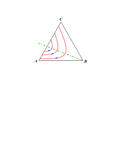
Figure 1: (Color online) Schematic plot of trajectories in the $(A,B,C)$ plane in case species $d$ dies first. The dashed red lines show the generalized hyperbolas (9) along which the system evolves by increasing A. At the intersections of the hyperbolas and the dot-dashed green lines $B$ is maximal.

III.2 A general criterion for survival/extinction

Turning to the full 4SS, we identify a single parameter that determines which of the pairs survive in the long time limit. To find this criterion, we note that eqns. (4-7) can be written as

$$\partial_{t}\ln A = k_{a}B-k_{d}D;\quad\partial_{t}\ln C=k_{c}D-k_{b}B$$ (13)

$$\partial_{t}\ln B = k_{b}C-k_{a}A;\quad\partial_{t}\ln D=k_{d}A-k_{c}C$$ (14)

since none of the fractions vanishes in finite $t$. This form is quite natural, since exponential growth/decay in populations is common. It also exposes clearly the coupling between the pairs $a$-$c$ and $b$-$d$. Constructing appropriate linear combinations, we showcase the contributions from a single species to the growth/decay of two other species:

$$\partial_{t}\left[k_{b}\ln A+k_{a}\ln C\right] = \lambda D$$

$$\partial_{t}\left[k_{c}\ln A+k_{d}\ln C\right] = \lambda B$$

$$\partial_{t}\left[k_{c}\ln B+k_{b}\ln D\right] = -\lambda A$$

$$\partial_{t}\left[k_{d}\ln B+k_{a}\ln D\right] = -\lambda C$$

where we have introduced the key control parameter

$$\lambda\equiv k_{a}k_{c}-k_{b}k_{d}\,\,.$$ (15)

Adding and subtracting appropriately, we see that the quantity

$$Q\equiv\frac{A^{k_{b}+k_{c}}C^{k_{d}+k_{a}}}{B^{k_{c}+k_{d}}D^{k_{a}+k_{b}}}$$ (16)

evolves in an extremely simple manner:

$$Q\left(t\right)=Q\left(0\right)e^{\lambda t}~{}.$$ (17)

The form of $Q$ also points to a simple interpretation of the behavior of the species. As in the card game, Bridge, $a$-$c$ and $b$-$d$ form opposing partner-pairs. For example, $a$’s action (consuming $b$) benefits $c$, while $c$’s action benefits $a$. Thus, we may refer to $a$-$c$ and $b$-$d$ as partners. Since no fraction can exceed unity, the only way for $Q$ to vanish or diverge is for one of the pairs to go extinct. Thus, the sign of $\lambda$ is the selection criterion for, and $Q$ is a quantitative measure of, which pair survives.

In this connection, we see that, unlike the 3SS Ber09 , the ‘weakest’ is not necessarily the survivor (or among the survivors) here. Indeed, if both members of a partner pair are weak (compared to their opponents), then the sign of $\lambda$ predicts the eventual demise of this pair, while the magnitude of $\lambda$ hints at how rapidly they will die out. As we have pointed out CDPZ-epl , the general maxim seems to be: “The prey of the prey of the weakest is the least likely to survive.” In the 3SS, this maxim also applies and is consistent with ‘survival of the weakest.’ There, ‘the prey of the prey of the weakest’ happens to be its predator, the demise of which naturally enhances its survival.

III.3 Saddle shaped orbits and fixed points for systems with $k_{a}k_{c}=k_{b}k_{d}$

Clearly, special properties will appear in a 4SS with $\lambda=0$, when $Q$ becomes an invariant. Indeed, there are two invariants Sza07 ; Dob10 ; CDPZ-epl . Neither pair goes extinct and the system evolves along periodic, closed orbits in configuration space. It is tempting to regard $Q$ as the generalization of the quantity $R\equiv A^{k_{b}}B^{k_{c}}C^{k_{a}}$ (introduced in Ber09 ) in the 3SS, except that $R$ is invariant for any set of rates. As will be shown in Section V, there are also fundamental differences between systems with even and odd number of cyclically competing species. As a result, direct comparisons between $R$ and $Q$ are not helpful, though both play important roles in identifying collective degrees of freedom that evolve trivially.

Proceeding to investigate the extra invariant besides $Q$, we find an appealing, symmetric way to display the two constants of motion:

$$f\equiv A^{k_{b}}C^{k_{a}}\quad\mbox{and}\quad g\equiv B^{k_{d}}D^{k_{a}}$$ (18)

(or equivalently, $f^{\prime}\equiv A^{k_{c}}C^{k_{d}}\quad$and$\quad g^{\prime}\equiv B^{k_{c}}D^{k_{b}}$). These generalize the products $AC$ and $BD$ in Sza07 , where the rates are all unity. Since invariants are fixed by the initial conditions ($f=A_{0}^{k_{b}}C_{0}^{k_{a}}$, etc.), it is natural to define the variables

$$\rho_{a} \equiv \left(A/A_{0}\right)^{k_{b}};\quad\rho_{c}\equiv\left(C/C_{0}\right)^{k_{a}}$$ (19)

$$\rho_{b} \equiv \left(B/B_{0}\right)^{k_{d}};\quad\rho_{d}\equiv\left(D/D_{0}\right)^{k_{a}}$$ (20)

Then, the constants of motion are simply the products:

$$\rho_{a}\rho_{c}=1;\quad\rho_{b}\rho_{d}=1~{}.$$ (21)

They define hyperbolic sheets through the tetrahedron and their intersection is a closed loop that resembles (the rim of) a saddle. Fig. 2a shows an example of such an orbit, for the case $k_{a}=0.4$, $k_{b}=0.4$, $k_{c}=0.1$, $k_{d}=0.1$. Here, the MFT eqns. (4-7) have been integrated numerically using a standard fourth-order Runge-Kutta scheme. Fig. 2b shows the ever-lasting oscillations in $A,...,D$ associated with this orbit.

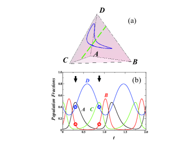
Figure 2: (Color online) (a) Example of a closed loop (solid curve) in the tetrahedron forming the configuration space, encircling the line of fixed points (green dashed line). Note that the fixed line bridges absorbing states on the $a$-$c$ and $b$-$d$ edges. The loop is generated by solving the mean field equations with a fourth order Runge-Kutta scheme, using time step $t=0.00001$. The rates $(k_{a},k_{b},k_{c},k_{d})$ used are $(0.4,0.4,0.1,0.1)$, yielding $\lambda=0$. (b) Evolution of the four species fractions as a function of time. The initial fractions $(A_{0},B_{0},C_{0},D_{0})$ are $(0.02,0.10,0.48,0.40)$. Next to each curve is its species label. The red and blue open circles mark the values of $B$ and $D$, respectively, associated with the two turning points of $A$, located by the black arrows. Note that both red (blue) circled values are the same. See text for details.

Many characteristics of a closed orbit in our tetrahedron are accessible analytically. We will summarize the findings here and defer the details to the Appendix. Let us start with the simplest: the average position (over one period, $T$):

$$\stackrel{{\scriptstyle\circ}}{{A}}\equiv\frac{1}{T}\int_{0}^{T}A\left(t\right)dt;\quad\stackrel{{\scriptstyle\circ}}{{B}}\equiv\frac{1}{T}\int_{0}^{T}B\left(t\right)dt;\quad etc.$$

Integrating eqns. (13,14), we find that the left vanish identically. Thus, we conclude

$$k_{a}\stackrel{{\scriptstyle\circ}}{{A}}=k_{b}\stackrel{{\scriptstyle\circ}}{{C}};\quad k_{a}\stackrel{{\scriptstyle\circ}}{{B}}=k_{d}\stackrel{{\scriptstyle\circ}}{{D}}\,\,.$$ (22)

Below, we will discuss the presence of a line of fixed-points for $\lambda=0$ systems, its properties given by the rates solely. It is perhaps not surprising that $\left(\stackrel{{\scriptstyle\circ}}{{A}},\stackrel{{\scriptstyle\circ}}{{B}},\stackrel{{\scriptstyle\circ}}{{C}},\stackrel{{\scriptstyle\circ}}{{D}}\right)$ lies on this line. Its precise location depends on the initial conditions, but finding this explicit dependence remains elusive. Another conclusion from this consideration is that all closed orbits enclose this non-trivial fixed line.

A more detailed description of our closed orbit is its projection onto, say, the $\rho_{a}$-$\rho_{d}$ plane. One possible representation is to exploit eqns. (19,20,3):

$$A_{0}\rho_{a}^{1/k_{b}}+B_{0}\rho_{d}^{-1/k_{d}}+C_{0}\rho_{a}^{-1/k_{a}}+D_{0}\rho_{d}^{1/k_{a}}=1\,\,.$$ (23)

In the Appendix, we will show how this ungainly looking equation can be transformed into the familiar equation for a circle: $\alpha^{2}+\beta^{2}=1$. We can gain some insight into this orbit by studying the extremal points. In particular, focusing on $A$ and $D$ of an orbit, we denote the extremes through the expressions:

$$A\in\left[A_{-},A_{+}\right],\qquad D\in\left[D_{-},D_{+}\right]\,\,.$$

These extremal points are given by the solution to the following equations:

$$A_{\pm}+J_{A}A_{\pm}^{-k_{b}/k_{a}} = 1-K_{A}\left(B_{0}^{k_{d}}D_{0}^{k_{a}}\right)^{1/\left(k_{a}+k_{d}\right)}$$ (24)

$$D_{\pm}+J_{D}D_{\pm}^{-k_{a}/k_{d}} = 1-K_{D}\left(A_{0}^{k_{b}}C_{0}^{k_{a}}\right)^{1/\left(k_{a}+k_{b}\right)}\,\,.$$ (25)

where $J$ and $K$ are constants:

$$J_{A} \equiv C_{0}A_{0}^{k_{b}/k_{a}},\quad J_{D}\equiv B_{0}D_{0}^{k_{a}/k_{d}}$$ (26)

$$K_{A} \equiv \left(\frac{k_{a}}{k_{d}}\right)^{k_{d}/\left(k_{a}+k_{d}\right)}+\left(\frac{k_{d}}{k_{a}}\right)^{k_{a}/\left(k_{a}+k_{d}\right)}$$ (27)

$$K_{D} \equiv \left(\frac{k_{b}}{k_{a}}\right)^{k_{a}/\left(k_{a}+k_{b}\right)}+\left(\frac{k_{a}}{k_{b}}\right)^{k_{b}/\left(k_{a}+k_{b}\right)}\,\,.$$ (28)

Being transcendental in general, these can be solved only numerically. Nevertheless, we can appreciate that there are typically two solutions to each (by a simple sketch of, say, $x+x^{-p}$). Obviously, the smaller (larger) of the two is the minimum (maximum). Interestingly, when a species is at its extremum, the fractions of its opposing partner-pair assume the same value. For example, when $A$ is at either turning point ($A_{\pm}$), $B$ takes on the same value, $\left[k_{d}^{k_{a}}k_{a}^{-k_{a}}B_{0}^{k_{d}}D_{0}^{k_{a}}\right]^{1/\left(k_{a}+k_{d}\right)}$. Similarly, $D$ takes on one value here: $\left[k_{a}^{k_{d}}k_{d}^{-k_{d}}B_{0}^{k_{d}}D_{0}^{k_{a}}\right]^{1/\left(k_{a}+k_{d}\right)}$. To illustrate, we mark one set in Fig. 2b with open circles. As will be discussed in Section IV, the minima $\left(A_{-},B_{-},C_{-},D_{-}\right)$ can play a role in predicting survivability in stochastic systems.

Finally, like the 3SS, there are non-trivial fixed points. Indeed, with one more degree of freedom than 3SS, we find a line of such points here. Note that these are neutrally stable, unlike the trivially time-independent, absorbing states. The simplest route to this line is to set the right of eqns. (4-7) to zero. Denoting the values on this line by $\left(A^{*},B^{*},C^{*},D^{*}\right)$, we see that they satisfy $k_{a}A^{*}=k_{b}C^{*}$ and $k_{a}B^{*}=k_{d}D^{*}$. In other words, the line is the intersection of the two planes. Exploiting $A+B+C+D=1$, we find an elegant way to display these values. Introducing a parameter $\gamma\in\left[0,1\right]$, we have

$$\left(A^{*},C^{*}\right)=\frac{\left(k_{b},k_{a}\right)}{k_{a}+k_{b}}\gamma;\quad\left(B^{*},D^{*}\right)=\frac{\left(k_{d},k_{a}\right)}{k_{a}+k_{d}}\left(1-\gamma\right)\,.$$ (29)

Clearly, this line is straight, and bridges the two absorbing states on the $a$-$c$ and $b$-$d$ lines, as illustrated in Fig. 2a. For the neighborhood of this line, it is natural to study linearized versions of eqns. (4-7). Writing $A=A^{*}+\Delta_{a}$ with $\Delta_{a}\ll A^{*}$, $B=B^{*}+\Delta_{b}$ with $\Delta_{b}\ll B^{*}$, etc., we first note that $\sum_{m}\Delta_{m}=0$ and $\partial_{t}\left(\Delta_{a}+\Delta_{c}\right)=0=\partial_{t}\left(\Delta_{b}+\Delta_{d}\right)$. Then, by defining $q\equiv k_{a}\Delta_{a}-k_{b}\Delta_{c}$ and $p\equiv k_{a}\Delta_{b}-k_{d}\Delta_{d}$, we can cast the linearized equations in the form of a standard simple harmonic oscillator: $\dot{q}=\left(k_{a}+k_{b}\right)A^{*}p;\,\,\dot{p}=-\left(k_{a}+k_{d}\right)B^{*}q$. In other words, the saddle-like orbits become planar while the system evolves along ellipses, with angular frequency $\sqrt{k_{b}k_{d}\gamma\left(1-\gamma\right)}$. Remarkably, contrary to natural expectations, the fixed line is not normal to the orbit plane in general.

To summarize, if $\lambda=0$, the evolution is relatively simple. Every starting point is associated with a closed, saddle-shaped orbit, on which the system remains forever. In general, analytic closed form expressions for them are not known (as far as we are aware). However, all enclose a fixed line and many of their properties can be computed analytically. Obviously, for finite systems evolving stochastically, these conclusions are valid only approximately – as long as the system is far from absorbing states.

III.4 Systems with $k_{a}k_{c}\neq k_{b}k_{d}$ : spirals and arrows

With such rates, $Q$ grows/decays exponentially, so that non-trivial fixed points cannot exist. Since all fractions are bounded by unity, this implies that either $BD$ or $AC$ vanishes in the large $t$ limit. In other words, for a system with finite $N$, extinction of one of the species must occur quite rapidly, especially if $\lambda$ is large. Before we continue to the analysis of these cases, let us provide a simple and intuitive picture, for appreciating the significance of $\lambda$.

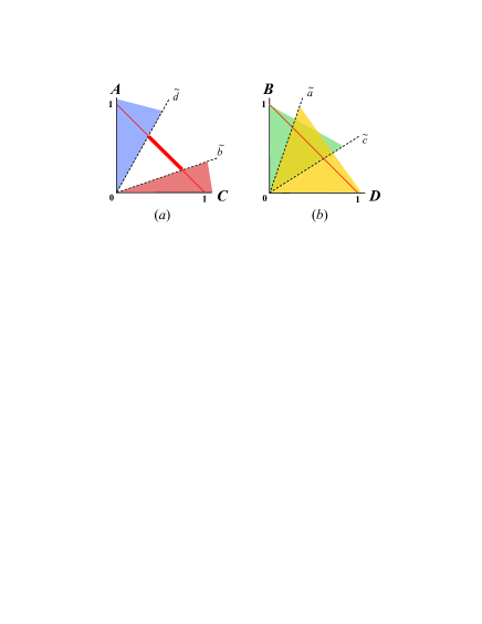
Figure 3: (Color online) (a) $A$-$C$ and (b) $B$-$D$ plane. When a trajectory enters the unshaded region in (a) and the doubly shaded region in (b), both $B$ and $D$ decrease whereas at the same time both $A$ and $C$ increase. See main text.

From eqns. (13,14), we see that the rise and fall of each species are associated with the relative values of the opposing pairs. For example, we can display a line in the $B$-$D$ plane ($k_{a}B=k_{d}D$, dashed line denoted by $\tilde{a}$ in Fig. 3b, on one side of which $A$ increases (shaded region, yellow online) and on the other, $A$ decreases. Of course, this ‘line’ is actually a plane in our configuration space tetrahedron. When the orbit crosses this plane, $A$ reaches a (local) extremum and turns around. A similar line ($k_{b}B=k_{c}D$; $\tilde{c}$ in Fig. 3b) can be plotted for the ‘divide’ between increasing (shaded region, green online) and decreasing $C$. The other set of lines, $\tilde{b}$ and $\tilde{d}$ in the $A$-$C$ plane, are shown in Fig. 3a. The significance of $\lambda$ is now clear. For $\lambda=0$, $\tilde{a}=\tilde{c}$, so that there are no regions where both $A$ and $C$ increase or decrease together. Meanwhile, we also have $\tilde{b}=\tilde{d}$ so that $B$ and $D$ also share such a property. By contrast, if $\lambda>0$, a ‘gap’ opens between these pairs of lines in such a way that in the region between $\tilde{a}$ and $\tilde{c}$, both $A$ and $C$ increase (e.g., overlap of shaded regions in Fig. 3b, a solid ‘wedge’ in the tetrahedron). On the other hand, in the region between $\tilde{b}$ and $\tilde{d}$, both $B$ and $D$ decrease (unshaded region in Fig. 3a). As a result, when the system gets into this domain (intersection of doubly-shaded and unshaded regions within our tetrahedron – i.e., an ‘irregular tetrahedron’), $B$ and $D$ will monotonically decrease, exponentially at late times. Simultaneously, $A$ and $C$ will monotonically increase, towards a final point $\left(A_{f},C_{f}\right)$ on the $a$-$c$ edge (solid diagonal line in Fig. 3a, red on line). In particular, the system will end on the heavy solid segment (red on line) of this line. In Fig. 4, we illustrate these features with such a ($\lambda>0$) case, showing a typical open orbit (starting at the solid circle, green online), spiralling towards an absorbing state on the $a$-$c$ edge (cross, red online).

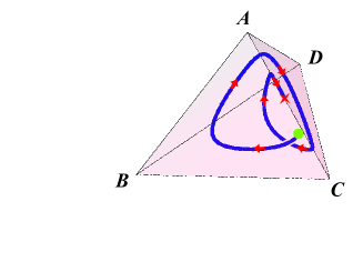
Figure 4: (Color online) Typical orbit for $\lambda>0$ that starts at the solid green circle and spirals towards an absorbing state, indicated by the red cross on the $a$-$c$ edge. The data shown here have been obtained for rates $k_{a}=0.45$, $k_{b}=0.33$, $k_{c}=0.14$, $k_{d}=0.08$ and initial fractions $A=0.02$, $B=0.10$, $C=0.48$, $D=0.40$.

To appreciate such monotonic behavior better, we present here a unique trajectory. Instead of being a spiral, it is as ‘straight as an arrow.’ A system started on this (straight) line will move along it for all $t$. In fact, as $\lambda\rightarrow 0$, this line becomes the fixed line (29) above. Here we simply quote the result. Readers interested in the origins and general characteristics of such ‘arrows’ will find details in Section Vb, which is devoted to systems with arbitrary (even) $S$. We start with an Ansatz for the fractions

$$\bar{A}h\left(t\right),\,\,\bar{B}\left[1-h\left(t\right)\right],\,\bar{C}h\left(t\right),\,\,\bar{D}\left[1-h\left(t\right)\right]$$ (30)

where $\bar{A},\bar{B},\bar{C},\bar{D}$ are constants. Clearly, these points lie on a straight line in the tetrahedron. For $h\in\left[0,1\right]$, this line joins the points $\left(\bar{A},0,\bar{C},0\right)$ and $\left(0,\bar{B},0,\bar{D}\right)$ on the $a$-$c$ and $b$-$d$ edges, respectively. Inserting these into eqns. (4,5), we find that they can be solved provided

$$\partial_{t}\ln h=\omega\left(1-h\right);\quad\partial_{t}\ln\left(1-h\right)=-\omega h$$

and

$$\omega=k_{a}\bar{B}-k_{d}\bar{D}=k_{c}\bar{D}-k_{b}\bar{B}=k_{a}\bar{A}-k_{b}\bar{C}=k_{c}\bar{C}-k_{d}\bar{A}\,$$

Thus, the result is

$$\left(\bar{A},\bar{B},\bar{C},\bar{D}\right)=\frac{\left(k_{b}+k_{c},k_{c}+k_{d},k_{a}+k_{d},k_{a}+k_{b}\right)}{k_{a}+k_{b}+k_{c}+k_{d}}$$ (31)

so that, explicitly,

$$\omega = \frac{k_{a}\left(k_{b}+k_{c}\right)-k_{b}\left(k_{a}+k_{d}\right)}{k_{a}+k_{b}+k_{c}+k_{d}}$$ (32)

$$= \frac{\lambda}{k_{a}+k_{b}+k_{c}+k_{d}}\,\,.$$ (33)

Since $h$ satisfies $dh/dt=\omega h\left(1-h\right)$, we may choose $h\left(0\right)=1/2$ and write the evolution along this straight trajectory explicitly:

$$h\left(t\right)=\frac{e^{\omega t}}{1+e^{\omega t}}~{}.$$ (34)

Note that, indeed, $h\in\left[0,1\right]$ for all $t$. Further, as $\lambda\rightarrow 0$, so does $\omega$ and $h$ become ‘frozen,’ playing the role of $\gamma$ in (29). Of course, in this limit, we easily see that, e.g., the ratio $\bar{A}/\bar{C}=\left(k_{b}+k_{c}\right)/\left(k_{a}+k_{d}\right)$ becomes $k_{b}\left(1+k_{d}/k_{a}\right)/\left(k_{a}+k_{d}\right)$ which is $k_{b}/k_{a}=A^{*}/C^{*}$. It is reassuring that this ‘arrow’ trajectory for $\lambda\neq 0$ is continuously linked to the fixed line in $\lambda=0$. Apart from this special line, all orbits (which we found numerically) spiral like a corkscrew, to various degrees, between the $a$-$c$ and $b$-$d$ edges. Classifying the characteristics of these spirals, a task well suited for future studies, will be highly non-trivial.

Whether we consider the arrow or spiraling trajectories, we remark that the time-reversed evolution (starting from any initial point) is also of interest. In this case, the opposite will occur: For systems with $\lambda>0$, say, $Q$ will decrease monotonically and the system ‘ends up’ somewhere on the opposite ($b$-$d$) edge. In this sense, the full dynamics for $\lambda\neq 0$ can be regarded as a family of spirals around an arrow, bridging the two opposite edges The initial condition simply serves to pick out the appropriate orbit, while the evolution consists of following it to an absorbing edge. Shown in Fig. 5 is such a spiral, but with two branches (black line vs. magenta [grey] line) corresponding to $t\rightarrow\pm\infty$ (starting at the same point). Underlying this dynamics appears to be a kind of ‘duality’ symmetry (associated with $\lambda,t\Leftrightarrow-\lambda,-t$). Exploring this aspect is likely a worthy pursuit, but clearly beyond the scope of this paper.

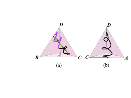
Figure 5: (Color online) A typical ‘arrow’ and spiral, with $\lambda=-0.0273$, from rates $(k_{a},k_{b},k_{c},k_{d})=(0.35,0.42,0.09,0.14)$. (a) Starting at the symmetry point (all fractions being $0.25$), the forward spiral is shown in magenta [grey]. The $t\rightarrow-\infty$ branch is shown as a black spiral. If started anywhere on the green arrow, the system will follow the arrow to the $b$-$d$ edge. (b) A different perspective of (both branches of) the same spiral.

IV Implications for stochastic evolution

When compared to the evolution of a fully stochastic 4SS with finite $N$, the predictions of the deterministic MFT can be a good approximation for the average behavior for cases with large $N_{m}$’s. Of course, MFT has serious limitations as well, apart from its inherent inability to describe fluctuations. The most glaring discrepancy lies with issues concerning extinction. Examples which readily come to mind are: What is the eventual extinction probability of a species? At what time is a species most likely to go extinct? And what is the average time for extinction? Since the fractions in MFT never vanish in finite time, none of these can be answered. Nevertheless, MFT can provide valuable insights Ber09 , some of which will be provided here. Extensive studies of the stochastic system and comparisons with MFT are beyond the scope of this article and will be presented in a subsequent publication CDPZ-JSTAT .

Let us consider first the $\lambda=0$ case, where only closed orbits prevail and all species survive in the MFT. This behavior resembles that in a 3SS. As pointed out in Ber09 , the closest approaches a closed loop makes with each edge (of the configuration space triangle) are good indicators of the survival probabilities. We should caution the reader that, in the 3SS triangle, an edge is associated with the survival of a single species, as well as the extinction of one other species. Thus, it is natural to associate a minimum distance to an edge ($\lambda_{m}$, in the notation of Ber09 ) with the survival of species $m$ (instead of the extinction of species $m-1$). In our case, the extinction of a species induces the survival of the opposing partner-pair. Thus, we find it more convenient to use the language of extinction of a species rather than likely survival of a pair. In other words, the closest approach to one of the four faces (in our tetrahedron) is a good indicator of the extinction probability of the associated species. For example, $A_{-}$ is the closest a loop comes within the face $A=0$, which corresponds to $a$ being extinct. Therefore, we can expect a species associated with the smallest in the set $\left(A_{-},B_{-},C_{-},D_{-}\right)$ to vanish first. In contrast to the 3SS case, the rates alone do not provide a useful criterion for extinction in our case, as we will show next.

In the 3SS, the initial conditions identifies a closed orbit and is associated with the invariant $R=A^{k_{b}}B^{k_{c}}C^{k_{a}}$. It is easy to find the closest approaches $\left(A_{-},B_{-},C_{-}\right)$ and to compute their ratios. For orbits with $R\ll 1$, these ratios are well approximated by

$$A_{-}/B_{-} \propto R^{1/k_{b}-1/k_{c}}\,\,~{},$$ (35)

$$B_{-}/C_{-} \propto R^{1/k_{c}-1/k_{a}}~{},$$ (36)

$$C_{-}/A_{-} \propto R^{1/k_{a}-1/k_{b}}~{}.$$ (37)

Notably, the proportionality coefficients depend only on the rates and not on $R$. Therefore, given a set of rates and a large population ($N\gg 1$), it is possible to arrive, through stochastic effects, at orbits where one of the fractions $N_{m}/N\rightarrow 1/N\ll 1$. Considering orbits with smaller and smaller $R$, we see that the above ratios will vanish or diverge, depending on the rates alone. For example, if $k_{a}<k_{b},k_{c}$ , then $C_{-}$ will be the smallest as $R\rightarrow 0$, so that $c$ is be the most likely to go extinct first. This argument leads to the conclusion in Ber09 : Extinction/survival probabilities are either zero or unity, in the limit of large $N$. By contrast, two invariants ($f=A^{k_{b}}C^{k_{a}},g=B^{k_{d}}D^{k_{a}}$) are associated with the closed loops in the 4SS. As a result, similar ratios of the closest approaches are not simple functions as in (35). Let us examine this issue further, by studying an example. We will again consider cases with small closest approaches, so that we can ignore the first term in eqn. (24) for finding, say, $A_{-}$. The results are

$$A_{-} \simeq f^{1/k_{b}}\left[1-K_{A}g^{1/\left(k_{a}+k_{d}\right)}\right]^{-k_{a}/k_{b}}$$

$$C_{-} \simeq f^{1/k_{a}}\left[1-K_{A}g^{1/\left(k_{a}+k_{d}\right)}\right]^{-k_{b}/k_{a}}$$

$$B_{-} \simeq g^{1/k_{d}}\left[1-K_{D}f\,\,^{1/\left(k_{a}+k_{b}\right)}\right]^{-k_{a}/k_{d}}$$

$$D_{-} \simeq g^{1/k_{a}}\left[1-K_{D}f\,\,^{1/\left(k_{a}+k_{b}\right)}\right]^{-k_{d}/k_{a}}$$

where $K_{A,D}$ are given by (27,28) and are independent of $f,g$. Even the ratios of each partner pair are not so clear-cut as in (35), since the ‘other invariant’ enters in a nontrivial way. For example, $g$ appears in the ratio

$$\frac{A_{-}}{C_{-}}\simeq f^{1/k_{b}-1/k_{a}}\left[1-K_{A}g^{1/\left(k_{a}+k_{d}\right)}\right]^{k_{b}/k_{a}-k_{a}/k_{b}}\,\,.$$

Needless to say, ‘cross-ratios’ such as $A_{-}/B_{-}$ are even more intractable. In a stochastic evolution, $f$ and $g$ presumably wander separately, so that it is a priori unclear which pair will win. Since the qualitative picture is already quite complex, we will not pursue the route in Ber09 where more quantitative arguments concerning scaling can be fruitful. Instead, devoting efforts towards the study of the full stochastics, along the lines of Dob10 , is likely to be more worthwhile.

Turning to systems with $\lambda\neq 0$, we can reach similar qualitative conclusions concerning how well the MFT predicts the behavior of the stochastic model. Here, $Q$ grows/decays exponentially and which pair survives is determined only by the sign of $\lambda$. Phrased in stark terms, this conclusion states that neither its magnitude nor the initial configuration (as long as they lie within the tetrahedron) plays a role. Clearly, this cannot be true for stochastically evolving, finite systems. From our simulations CDPZ-JSTAT , we glean another maxim: “The prey of the prey of the strongest is quite likely to survive.” Although this principle appears to be the same as the one posed above (albeit a double-negative version), the consequences for the end state can be drastically different. In particular, both $\left|\lambda\right|$ and the initial conditions, as well as the total population size, can reverse the predictions of MFT. Let us illustrate with the example in CDPZ-epl with ‘extreme’ rates: $k_{m}=\left(0.1,0.001,0.1,0.7999\right)$. Since $\lambda>0$, $a$-$c$ is predicted to win. When the initial population is set at $N_{m}=\left(100,700,100,100\right)$, 90% of the runs indeed end with the $a$-$c$ pair. However, for a symmetric starting point of $N_{m}=\left(100,100,100,100\right)$, 97% of the runs end with $b$ as the sole survivor, despite the initial $N_{b}$ being much smaller! To accommodate these two very different outcomes, we apply the two different maxims. As $b$ is the weakest and $d$ is the strongest, each is the prey of the other’s prey. In one case, the first maxim lead us to $D$ vanishing first, leaving us with $a$-$c$ coexistence. In the second scenario, $d$ consumes $a$ so rapidly that $A$ vanishes first and $b$ can only increase. But $b$ is slow to consume $c$, so that $d$ goes extinct next. As a result, $b$ is the only survivor (rather than one of the more numerous states of $b$-$d$ coexistence). To turn these qualitative considerations into quantitative conclusions, concerning the detail interplay between the rates and the initial configuration, will be a serious challenge.

To summarize this section, let us reiterate that, while MFT cannot predict all eventualities of a finite stochastic system, it can provide some hints. Specifically, the proximity of an MFT trajectory to an absorbing face should be a good guide for the extinction probabilities of the associated species. For the 3SS, this guide led to very successful predictions, i.e., survival of the weakest. This success can be traced to the presence of only a few degrees of freedom, so that, along with the existence of the invariant $R$, the rates alone determine the relative proximity of the orbits to the three extinction lines. By contrast, the 4SS is sufficiently more complex that similar conclusions cannot be drawn.

V Systems with $S$ species

In this section, we present extensions of our findings to a system of $N$ individuals consisting of an arbitrary number, $S$, of cyclically competing species. This generalization provides some insight into the general structure of the dynamics in such systems. In particular, these considerations lead us to the deeper origins of the existence of collective variables like $R$ and $Q$, as well as fixed points and ‘arrows.’ For any odd $S$, we show that there is precisely one (non-trivial) fixed point and one $R$-like invariant. By contrast, for even $S$, a $Q$-like quantity (evolving simply as an exponential) and an ‘arrow’ trajectory always exist. Regarding the system as two opposing teams, we show that the winners always have the larger rates-product (e.g., $a$-$c$ if $k_{a}k_{c}$ is larger). When the competition is neutral (equal rate-products), there will always be a fixed line and two $R$-like invariants.

Following Section II, we now consider the species $x_{m}$ ($m=1,\cdots,S$) interacting cyclically:

$$x_{m}+x_{m+1}\stackrel{{\scriptstyle p_{m}}}{{\rightarrow}}2x_{m}$$ (38)

(with $x_{S+1}=x_{1}$). The rate equations for the fractions $X_{m}\equiv N_{m}/N$ take the form

$$\partial_{t}X_{m}=\left[k_{m}X_{m+1}-k_{m-1}X_{m-1}\right]X_{m}~{}.$$ (39)

Of course, $\sum_{m}X_{m}=1$, so that our configuration space is an $S-1$ simplex (a hyper-tetrahedron). As in Section III, a better approach is to cast eqn. (39) as

$$\partial_{t}\left(\ln X_{m}\right)=k_{m}X_{m+1}-k_{m-1}X_{m-1}~{}.$$ (40)

Despite the non-linearity, we will find it convenient to exploit the notation of vectors and matrices. Thus, we rewrite this equation as

$$\partial_{t}\overrightarrow{\ln X}=\mathbb{K}\vec{X}$$ (41)

where

$$\mathbb{K}=\left(\begin{array}[]{cccccc}0&k_{1}&0&...&0&-k_{S}\\ -k_{1}&0&k_{2}&...&0&0\\ 0&-k_{2}&0&...&0&0\\ \vdots&\vdots&\vdots&...&\vdots&\vdots\\ 0&0&0&...&0&k_{S-1}\\ k_{S}&0&0&...&-k_{S-1}&0\end{array}\right)$$ (42)

is an antisymmetric, cyclic matrix and $\vec{X}$ is a vector with elements $X_{m}$. Introducing

$$\vec{E}=\left(\begin{array}[]{ccccc}1&1&...&1&1\end{array}\right)$$

we see that $\sum_{m}X_{m}=1$ is simply $\vec{E}\cdot\vec{X}=1$. The significance of eqn. (41) is clear: It highlights the difference between having a singular $\mathbb{K}$ or not. Such properties are best explored by considering systems with odd/even $S$ separately. Indeed, the major differences between the 3SS and 4SS can be understood in the light of this even/odd distinction. (Odd-even effects were briefly discussed in Sat02 for systems on a two-dimensional lattice).

V.1 Systems with odd $S$

Antisymmetric matrices have a simple property: If $\kappa$ is an eigenvalue, then so is $-\kappa$. Since $S$ is odd, there must be at least one eigenvalue which is zero (the rest being pairs of opposite signs). Indeed, our $\mathbb{K}$ has only one such eigenvalue, as shown in Appendix B, so that its null space is one-dimensional. The associated right eigenvector, $\vec{\zeta}$, satisfies $\mathbb{K}\vec{\zeta}=0$. All its elements, $\zeta_{m}$, can be chosen to be positive, since they obey $k_{m-1}\zeta_{m-1}=k_{m}\zeta_{m+1}$. Of course, when normalized appropriately, it becomes the fixed point population:

$$\vec{X}^{*}=\frac{\vec{\zeta}}{\vec{E}\cdot\vec{\zeta}}~{}.$$ (43)

Since $\mathbb{K}$ is antisymmetric, $\vec{\zeta}$ is also the left eigenvector ($\vec{\zeta}\cdot\mathbb{K}=0$). Thus, we arrive at $\partial_{t}\vec{\zeta}\cdot\overrightarrow{\ln X}=0$, which leads us to define an invariant

$$\mathcal{R}\equiv\prod_{m}X_{m}^{\zeta_{m}}\,\,.$$ (44)

Note that $\vec{\zeta}$ is determined up to an overall constant, which simply corresponds to $\mathcal{R}$ being fixed (up to an overall power). This is the generalization of $R$ in the 3SS. Together with $\vec{E}\cdot\vec{X}=1$, this invariant defines a compact, $S-2$ dimensional manifold on which the orbit must lie. We find it remarkable that $\vec{\zeta}$ plays a ‘dual’ role, serving to pinpoint both the fixed point $\vec{X}^{*}$ and to define the invariant $\mathcal{R}$. An interesting question naturally arises: Does a deeper connection between these apparently unrelated quantities exist?

V.2 Systems with even $S$

We may regard such systems as the competition between two ‘teams,’ each with $s\equiv S/2$ species. In particular, this aspect becomes transparent if we reorder our species to

$$X_{1},X_{3},...,X_{S-1},X_{2},...,X_{S}$$

and define ‘team variables’

$$Y_{\ell}\equiv X_{2\ell-1};\quad Z_{\ell}\equiv X_{2\ell}$$

with $\ell=1,...,s$. In terms of these, the matrix $\mathbb{K}$ takes the form

$$\mathbb{K}=\left(\begin{array}[]{cc}0&\mathbb{M}\\ -\mathbb{M}^{\text{T}}&0\end{array}\right)$$ (45)

and eqn. (41) becomes

$$\partial_{t}\left(\begin{array}[]{c}\overrightarrow{\ln Y}\\ \overrightarrow{\ln Z}\end{array}\right)=\left(\begin{array}[]{cc}0&\mathbb{M}\\ -\mathbb{M}^{\text{T}}&0\end{array}\right)\left(\begin{array}[]{c}\vec{Y}\\ \vec{Z}\end{array}\right)\,.$$ (46)

Of course, the full space and ‘team space’ have different dimensions ($S$ vs. $s$), but using the same notation ($\mathbb{K}$, $\mathbb{M}$, $\vec{X}$, $\vec{Y}$, etc.) should not cause much confusion. Note that eqn. (46) exposes a simplectic structure that is typical in the ‘competition of two (sets of) variables.’

Careful accounting of the $s\times s$ matrix $\mathbb{M}$ leads to:

$$\mathbb{M}=\left(\begin{array}[]{ccccc}k_{1}&0&...&0&-k_{S}\\ -k_{2}&k_{3}&...&0&0\\ 0&-k_{4}&...&0&0\\ \vdots&\vdots&...&\vdots&\vdots\\ 0&0&...&-k_{S-2}&k_{S-1}\end{array}\right)$$ (47)

Note that its structure is quite different from $\mathbb{K}$, with the (even) odd rates lining the (sub-)diagonal. Whether $\mathbb{K}$ is singular or not is just controlled by $\Lambda\equiv\det\mathbb{M}$. A straightforward computation leads to

$$\Lambda=\prod_{odd\,\,m}k_{m}-\prod_{even\,\,m}k_{m}$$

regardless of whether $s$ is even or odd. Clearly, $\Lambda$ is the generalization of $\lambda$ in the 4SS and its sign determines which team wins. If $\Lambda\neq 0$, $\mathbb{K}^{-1}$ exists so that $\partial_{t}\left[\vec{E}\cdot\mathbb{K}^{-1}\overrightarrow{\ln X}\right]=\vec{E}\cdot\vec{X}=1$. Denoting $\sum_{j}\left(K^{-1}\right)_{jm}$ by $\sigma_{m}$ and defining

$$\mathcal{Q}\equiv\exp\left[\vec{E}\cdot\mathbb{K}^{-1}\overrightarrow{\ln X}\right]=\prod_{m}X_{m}^{\sigma_{m}}$$ (48)

we see that it evolves trivially: $\mathcal{Q}\left(0\right)e^{t}$. Of course, it is impossible to form such teams in systems with odd $S$, there is no $\mathcal{Q}$-like variable, and this simple scenario is invalid.

Though obviously related to $Q$ in the 4SS, $\mathcal{Q}$ is less transparent, since $e^{t}$ obscures the $\Lambda$ dependence of our system! To find the generalization of $Q$ and to shed light on the $\Lambda\rightarrow 0$ limit, we exploit the team variables $\left(\vec{Y},\vec{Z}\right)$ and consider $\mathbb{W}$, the cofactors of $\mathbb{M}$. Unlike $\mathbb{M}^{-1}$,

$$\mathbb{W}=\Lambda\mathbb{M}^{-1}$$ (49)

is well behaved even when $\Lambda=0$. Multiplying eqn. (46) by

$$\left(\begin{array}[]{cc}0&-\mathbb{W}^{\text{T}}\\ \mathbb{W}&0\end{array}\right)$$ (50)

we have

$$\partial_{t}\left(\begin{array}[]{c}-\mathbb{W}^{\text{T}}\,\overrightarrow{\ln Z}\\ \mathbb{W}\,\overrightarrow{\ln Y}\end{array}\right)=\Lambda\left(\begin{array}[]{c}\vec{Y}\\ \vec{Z}\end{array}\right)~{}.$$ (51)

Now, a tedious computation shows that all the matrix elements of $\mathbb{W}$ are positive (sums of products of $s-1$ rates, e.g., $k_{b}+k_{c}$ in the $s=2$ case above). Let us define the following positive quantities

$$q_{\ell}\equiv\sum_{n}W_{n\ell};\quad r_{n}\equiv\sum_{\ell}W_{n\ell}$$ (52)

which are readily recognized as $\vec{E}\cdot\mathbb{W}$ and $\vec{E}\cdot\mathbb{W}^{\text{T}}$, respectively. Thus, by taking the scalar product of $\vec{E}$ with eqn. (51), we are led to the combination

$$Q\equiv\exp\left[\vec{q}\cdot\overrightarrow{\ln Y}-\vec{r}\cdot\overrightarrow{\ln Z}\right]=\left.\prod_{\ell}Y_{\ell}^{q_{\ell}}\right/\prod_{\ell}Z_{\ell}^{r_{\ell}}$$ (53)

which evolves according to

$$Q\left(t\right)=Q\left(0\right)e^{\Lambda t}\,\,.$$ (54)

To help the readers, let us connect these results to the 4SS case explicitly. There,

$$\left(\begin{array}[]{c}\vec{Y}\\ \vec{Z}\end{array}\right)=\left(\begin{array}[]{c}A\\ C\\ B\\ D\end{array}\right)$$

and

$$\mathbb{M}=\left(\begin{array}[]{cc}k_{a}&-k_{d}\\ -k_{b}&k_{c}\end{array}\right);\quad\Lambda=\lambda;\quad\mathbb{W}=\left(\begin{array}[]{cc}k_{c}&k_{d}\\ k_{b}&k_{a}\end{array}\right)$$

so that all the conclusions reached in Section III are recovered.

As in the 4SS, the orbits are, in general, analytically inaccessible. However, the ‘straight arrow’ trajectory can be determined explicitly, while the time dependence along it remains the same for any number of species. In particular, we begin with the most trivial case: $s=1=S/2$:

$$\partial_{t}X_{1}=k_{1}X_{1}X_{2};\quad\partial_{t}X_{2}=-k_{1}X_{1}X_{2}$$ (55)

so that $\Lambda$ is just $k_{1}$. and $Q=X_{1}/X_{2}\propto e^{k_{1}t}$. Since $X_{2}=1-X_{1}$, the solution is trivial, being the same form as (34) with $k_{1}$ in place of $\omega$. As $t$ runs to $-\infty$ or $+\infty$, it reaches the two terminals $X_{1}=1$ or $X_{2}=1$. Turning to general $S$, we seek such a straight line, bridging the terminal points ($\bar{Y}_{\ell}$ and $\bar{Z}_{\ell}$) in the subspaces of each team, that can serve as a $t$-dependent trajectory. Making the same Ansatz as in eqn. (30), let us consider

$$\bar{Y}_{\ell}h\left(t\right),\,\bar{Z}_{\ell}\left[1-h\left(t\right)\right]$$

which runs from $\left(\bar{Y}_{\ell},0\right)$ to $\left(0,\bar{Z}_{\ell}\right)$. We will also assume the same $h\left(t\right)$ as in (34), except for $\omega$ being replaced by $\Omega$, a parameter to be determined. Inserting these into the left of eqn. (46), we find

$$\left(\begin{array}[]{c}\vec{E}\,\partial_{t}\ln h\\ \vec{E}\,\partial_{t}\ln\left[1-h\right]\end{array}\right)=\Omega\left(\begin{array}[]{c}\vec{E}\left(1-h\right)\\ -\vec{E}\,h\end{array}\right)~{}.$$ (56)

Meanwhile the right of eqn. (46) is

$$\left(\begin{array}[]{c}\mathbb{M}\,\vec{Z}\\ -\mathbb{M}^{\text{T}}\,\vec{Y}\end{array}\right)=\left(\begin{array}[]{c}\vec{\Xi}\left(1-h\right)\\ -\vec{\Upsilon}\,h\end{array}\right)$$ (57)

where the components of $\vec{\Upsilon}$ and $\vec{\Xi}$ on the right are, respectively,

$$\sum_{\ell}M_{\ell n}\bar{Y}_{\ell}\quad\text{and}\quad\sum_{\ell}M_{n\ell}\bar{Z}_{\ell}~{}.$$ (58)

Setting expressions (56,57) equal, we find

$$\bar{Y}_{n} = \Omega\sum_{\ell}\left(M^{-1}\right)_{\ell n}~{},$$

$$\bar{Z}_{n} = \Omega\sum_{\ell}\left(M^{-1}\right)_{n\ell}~{}.$$

Exploiting (49,52), we have

$$\bar{Y}_{n} = \frac{\Omega}{\Lambda}\sum_{\ell}W_{\ell n}=\frac{\Omega}{\Lambda}q_{n}~{},$$ (59)

$$\bar{Z}_{n} = \frac{\Omega}{\Lambda}\sum_{\ell}W_{n\ell}=\frac{\Omega}{\Lambda}r_{n}~{}.$$ (60)

Now, all details for our ‘arrow’ condition are fixed, by imposing $\sum_{n}\bar{Y}_{n}=1$ etc. The result is

$$\Omega=\Lambda\left/\sum_{n,\ell}W_{\ell n}\right.$$ (61)

i.e., the generalization of (33).

We end with some remarks on the cases with $\Lambda=0$. Although properties of these can be found by taking the $\Lambda\rightarrow 0$ limit of the above, let us provide a more direct route. Since $S$ is even, a zero eigenvalue of $\mathbb{K}$ is doubly degenerate and the null space is two-dimensional (at the least). Given the form (45), we see that this null space is determined by the right eigenvectors of $\mathbb{M}$ and $\mathbb{M}^{\text{T}}$:

$$\mathbb{M}\,\vec{\xi}=0=\mathbb{M}^{\text{T}}\vec{\eta}\,~{}.$$

We can impose the constraint and define fixed points within the space of each ‘team’:

$$Y_{\ell}^{*}=\xi_{\ell}\left/\sum_{n=1}^{s}\xi_{n}\right.;\quad Z_{\ell}^{*}=\eta_{\ell}\left/\sum_{n=1}^{s}\eta_{n}\right.~{}.$$

Joining these is a fixed line in the full $S-1$ simplex, that can be parametrized in the same manner as in eqn. (29) of the 4SS:

$$\left(\begin{array}[]{c}\vec{Y}^{*}\\ \vec{0}\end{array}\right)\gamma+\left(\begin{array}[]{c}\vec{0}\\ \vec{Z}^{*}\end{array}\right)\left(1-\gamma\,\,\right)\,\,.$$

Meanwhile, the left eigenvectors of $\mathbb{K}$, are expected to play a ‘dual’ role, as in the odd $S$ cases. Of course, these can be formed from $\vec{\eta}$ and $\vec{\xi}$, which are the left eigenvector of $\mathbb{M}$ and $\mathbb{M}^{\text{T}}$, respectively. The results are $\left(\vec{\eta},\vec{0}\right)$ and $\left(\vec{0},\vec{\xi}\right)$, which can now be exploited to define the generalizations of $f$ and $g$, see eq. (18): $\vec{\eta}\cdot\overrightarrow{\ln Y}$ and $\vec{\xi}\cdot\overrightarrow{\ln Z}$. Not surprisingly, these are intimately related to the numerator and the denominator in expression (53). Note that the sum $\vec{\eta}\cdot\overrightarrow{\ln Y}+\vec{\xi}\cdot\overrightarrow{\ln Z}$ is also an invariant. Exponentiating it will produce a quantity which has the appearance of $\mathcal{R}$, i.e., products of only positive powers of $X_{m}$. For systems with all interaction rates being equal, such an invariant takes an appealing form: $X_{1}X_{2}...X_{S}$ (for any $S$). Finally, we note that $\mathbb{M}$ has no other zero eigenvalues (shown in Appendix B), so that there are no other invariants. Thus, the orbits lie in a compact, $S-3$ dimensional manifold in general. Of course, for $S=4$, the 1-dimensional manifolds are simply closed loops, for which many properties are explicitly obtained in Section III. For $S>4$, we have not found similar explicit characteristics.

VI Summary and outlook

In an effort to understand better the counter-intuitive phenomenon of “survival of the weakest,” which was discovered in recent studies of a well-mixed system involving three cyclically competing species, we investigate a system with four species. In a previous letter CDPZ-epl , we reported preliminary findings, showing that this behavior does not persist. Instead, all systems seem to follow an intuitively understandable principle: “The prey of the prey of the weakest is most likely to go extinct first.” In a 3SS, this species is also the predator of the weakest, and so, its early demise leads to the weakest being the sole survivor. By contrast, the players in a 4SS form partner-pairs, much like in the game of Bridge. As a result, our new maxim hints that the weaker pair is not likely to survive. All these studies consist of two aspects, each of interest on their own. The first is mean field theory (MFT), i.e., non-linear dynamics of a set of deterministic rate equations. The second is the stochastic evolution of a finite population of $N$ individuals. For the 4SS, we show how the former, our set of rate equations: (4)-(7), arises from the master equation which defines the latter. This article is devoted to an in-depth exploration of the MFT, i.e., solutions to the rate equations.

Since the evolution of the 4SS takes place within a tetrahedron, it is more complex than the 3SS case. Nevertheless, we are able to obtain considerable details analytically, mainly through the discovery of hidden symmetries. Not surprisingly, far fewer exact results of the stochastic aspect are attainable. Instead, most insight into this behavior is gained through computer simulations. Indeed, in some ‘extreme’ cases, we found that the outcomes contradict the MF prediction completely CDPZ-epl . Instead, these can be understood by a complementary version of the above maxim, namely, “The prey of the prey of the strongest is most likely to survive.” A similar, in-depth investigation of the second aspect (stochastic evolution) is beyond the scope here, and those results will be reported elsewhere CDPZ-JSTAT .

Unlike the 3SS, in which all MFT orbits are closed loops (characterized by $R$) in a plane, the 4SS supports a richer variety of trajectories. The details depend on the initial conditions and the rates, especially through $\lambda=k_{a}k_{c}-k_{b}k_{d}$. We show that, provided they start within our tetrahedron, all orbits spiral, to various degrees, into the $a$-$c$ edge ($\lambda>0$) or the $b$-$d$ edge ($\lambda<0$). There is one exception, namely, a special straight line bridging the two edges. On it the system moves monotonically, leading us to refer to it as the ‘arrow.’ In general, the spirals wrap around this arrow. To describe the motion along the spirals and the arrow quantitatively, we find a collective variable, $Q$, which evolves simply as an exponential, see eqns. (16,17). Indeed, letting $t$ run from $-\infty$ to $\infty$, we see that these trajectories all start on one edge ($a$-$c$ or $b$-$d$) and end on the opposite one. As $\left|\lambda\right|\rightarrow 0$, the spirals become tighter (lower pitched) so that, for $\lambda=0$, all orbits are closed loops which resemble the edge of a saddle. Meanwhile, the ‘arrow’ becomes a line of fixed points, around which all closed orbits encircle. In addition to $Q$, another invariant emerges. Together, these two, see eq. (18), completely specify the saddle shaped loops. Though the explicit forms are not available, many properties of these loops, e.g., maximal extent in principle directions, have been found. Finally, by extending these considerations to cyclic competition of an arbitrary number, $S$, of species, we can trace the origins of these special quantities (invariants, collective variables, non-trivial fixed points and lines, etc.) to general properties of an $S\times S$ antisymmetric, cyclic matrix, $\mathbb{K}$. The elements of $\mathbb{K}$ are just the rates, so that all details of these special quantities are explicitly known. Indeed, a recent study finds that such ‘hidden symmetries’ are present in an even wider class of systems involving competing species Zia10 . Of course, as our scope broadens, fewer explicit results are available.

Let us reiterate that the main forte of MFT is to provide reliable estimates of the evolution when the population of every species is large. Relying on continuous fractions (and continuous time), it fares poorly when one or more species are near extinction and their numbers drop to $O\left(1\right)$. Though it fails to predict all eventualities of a finite stochastic system, it does give us some useful hints. Specifically, the proximity of an MFT trajectory to an absorbing face should be a good guide for the extinction probabilities of the associated species. We have not systematically explore this issue and such an undertaking seems worthwhile.

Beyond such immediate questions, we believe there are interesting avenues for further research. We end with pointing out a few here. The sheets labeled by $\tilde{a}$, $\tilde{b}$, etc. are clearly significant, as they correspond to the turning points of species $a$, $b$, etc. It seems likely that these are good candidates for Poincaré sections with which to analyze our dynamical system. How often orbits pierce these sheets may also serve to classify the spirals by the total number of turns, $\chi$ (‘windings’), between the end points. Clearly, $\chi$ is zero for the arrow, while our expectation is that this value will be infinitesimal for a spiral in its neighborhood. In other words, a perturbative approach is likely to be successful. Of course, to be quantitative, we should look for a good coordinate system for configuration space, guided by slow and fast dynamics, along the lines of action-angle variables in classical mechanics. For the neutral cases ($\lambda=0$), these have been identified: $f,g,\theta$ in eqns. (18, 68). In the general case, we already have one key variable, $Q$. It seems quite feasible to find two others, perhaps in analog to a radius (distance from the arrow) and an angle, $\phi$. Once their $t$-dependence is established, then the classification of orbits we conjectured would be realized by $\chi\equiv\phi\left(t=\infty\right)-\phi\left(t=-\infty\right)$. It is even conceivable that a deeper connection with similar concepts in scattering theory exists.

Appendix A Properties of closed orbits

Quantitative details of a closed orbit can be found through its projection onto, say, the $\rho_{a}$-$\rho_{d}$ plane. Using $A=A_{0}\rho_{a}^{1/k_{b}}$, etc., the (generically transcendental) equation for this projection is given by eqn. (23):

$$A_{0}\rho_{a}^{1/k_{b}}+B_{0}\rho_{d}^{-1/k_{d}}+C_{0}\rho_{a}^{-1/k_{a}}+D_{0}\rho_{d}^{1/k_{a}}=1\,\,.$$

Clearly, this is just one of many equivalent representations. We begin with finding the extremal points of this closed loop. Exploiting such points, we can transform this cumbersome equation into a familiar one, (67) below. Finally, we will show how the period of these orbits can be found, explicitly in certain cases.

To find the extremal points, let us first consider the combination involving $\rho_{a}$:

$$F\left(\rho_{a}\right)\equiv A_{0}\rho_{a}^{1/k_{b}}+C_{0}\rho_{a}^{-1/k_{a}}\,\,.$$

As $F$ is convex, it has a unique minimum value, $\stackrel{{\scriptstyle\vee}}{{F}}$, which occurs at

$$\stackrel{{\scriptstyle\vee}}{{\rho}}_{a}\equiv\left[\frac{k_{b}C_{0}}{k_{a}A_{0}}\right]^{\frac{k_{a}k_{b}}{k_{a}+k_{b}}}\,\,,$$

and corresponds to

$$\stackrel{{\scriptstyle\vee}}{{A}}=A_{0}\stackrel{{\scriptstyle\vee}}{{\rho}}_{a}^{1/k_{b}}=\left[k_{b}^{k_{a}}k_{a}^{-k_{a}}A_{0}^{k_{b}}C_{0}^{k_{a}}\right]^{1/\left(k_{a}+k_{b}\right)}~{}.$$

In other words, $F\left(\stackrel{{\scriptstyle\vee}}{{\rho}}_{a}\right)=\stackrel{{\scriptstyle\vee}}{{F}}$. Similarly, the other combination,

$$G\left(\rho_{d}\right)\equiv B_{0}\rho_{d}^{-1/k_{d}}+D_{0}\rho_{d}^{1/k_{a}}$$

has a minimum, $\stackrel{{\scriptstyle\vee}}{{G}}$, occurring at

$$\stackrel{{\scriptstyle\vee}}{{\rho}}_{d}\equiv\left[\frac{k_{d}B_{0}}{k_{b}D_{0}}\right]^{\frac{k_{a}k_{d}}{k_{a}+k_{d}}}\,\,\Leftrightarrow\,\,\stackrel{{\scriptstyle\vee}}{{D}}=\left[k_{a}^{k_{d}}k_{d}^{-k_{d}}B_{0}^{k_{d}}D_{0}^{k_{a}}\right]^{1/\left(k_{a}+k_{d}\right)}$$

Although neither $F$ nor $G$ are functions bounded from above, the constraint $F+G=1$ does impose upper bounds in this context. Thus, we find the largest value $F$ can take must be given by $\stackrel{{\scriptstyle\wedge}}{{F}}=1-\stackrel{{\scriptstyle\vee}}{{G}}$ . Similarly, we have $\stackrel{{\scriptstyle\wedge}}{{G}}=1-\stackrel{{\scriptstyle\vee}}{{F}}$ . While $\stackrel{{\scriptstyle\wedge}}{{F}}$ and $\stackrel{{\scriptstyle\wedge}}{{G}}$ are unique, each is associated with two points, in $A$ and $D$ (or $\rho_{a}$ and $\rho_{d}$). Labeling these pairs by $A_{\pm}$ and $D_{\pm}$, we see their significance: They are the extremal points of the orbit, i.e.,

$$A\in\left[A_{-},A_{+}\right],\qquad D\in\left[D_{-},D_{+}\right]~{}.$$

Let us emphasize that $A_{-},D_{-}\neq\stackrel{{\scriptstyle\vee}}{{A}},\stackrel{{\scriptstyle\vee}}{{D}}$ in general: The former is the lower bound for $A$ while the latter is associated with the minimum of $F$.

Next, we study the defining equations for the extremal points:

$$F\left(A_{\pm}\right)=1-\stackrel{{\scriptstyle\vee}}{{G}},\qquad G\left(D_{\pm}\right)=1-\stackrel{{\scriptstyle\vee}}{{F}}.$$

These give rise to eqns. (24-28) in Section IIIc, reproduced here for convenience:

$$A_{\pm}+J_{A}A_{\pm}^{-k_{b}/k_{a}} = 1-K_{A}\left(B_{0}^{k_{d}}D_{0}^{k_{a}}\right)^{1/\left(k_{a}+k_{d}\right)}$$ (62)

$$D_{\pm}+J_{D}D_{\pm}^{-k_{a}/k_{d}} = 1-K_{D}\left(A_{0}^{k_{b}}C_{0}^{k_{a}}\right)^{1/\left(k_{a}+k_{b}\right)}\,\,.$$ (63)

with

$$J_{A} \equiv C_{0}A_{0}^{k_{b}/k_{a}},\quad\,J_{D}\equiv B_{0}D_{0}^{k_{a}/k_{d}}$$ (64)

$$K_{A} \equiv \left(\frac{k_{a}}{k_{d}}\right)^{k_{d}/\left(k_{a}+k_{d}\right)}+\left(\frac{k_{d}}{k_{a}}\right)^{k_{a}/\left(k_{a}+k_{d}\right)}$$ (65)

$$K_{D} \equiv \left(\frac{k_{b}}{k_{a}}\right)^{k_{a}/\left(k_{a}+k_{b}\right)}+\left(\frac{k_{a}}{k_{b}}\right)^{k_{b}/\left(k_{a}+k_{b}\right)}\,\,.$$ (66)

Let us reiterate: When a species is at its maximum or its minimum, the fractions of its opposing partner-pair assume the same value. Thus, when $A=A_{\pm}$, $B$ takes on the same value: $\stackrel{{\scriptstyle\vee}}{{B}}=\left(k_{d}^{k_{a}}k_{a}^{-k_{a}}B_{0}^{k_{d}}D_{0}^{k_{a}}\right)^{1/\left(k_{a}+k_{d}\right)}$ while $D$ assumes the value $\stackrel{{\scriptstyle\vee}}{{D}}$.

The other pairs of extremal points ($B_{\pm},C_{\pm}$) can be similarly studied. But, it is much simpler to exploit the invariant $f,g$ and to recognize that the extremal points are paired, so that

$$C_{\pm}=\left(\left.f\right/A_{\mp}^{k_{b}}\right)^{1/k_{a}},\qquad B_{\pm}=\left(\left.g\right/D_{\mp}^{k_{a}}\right)^{1/k_{d}}\,\,.$$

Though the solutions to equations like (24) should provide some indications of the extent of the saddle shaped orbits, our goal is the simple form (23) of the orbit equation. We begin with the observation that both $F\left(\rho_{a}\right)-\stackrel{{\scriptstyle\vee}}{{F}}$ and $G\left(\rho_{d}\right)-\stackrel{{\scriptstyle\vee}}{{G}}$ lie in the range $\left[0,M\right]$, where

$$M\equiv\stackrel{{\scriptstyle\wedge}}{{F}}-\stackrel{{\scriptstyle\vee}}{{F}}=1-\stackrel{{\scriptstyle\vee}}{{G}}-\stackrel{{\scriptstyle\vee}}{{F}}=\stackrel{{\scriptstyle\wedge}}{{G}}-\stackrel{{\scriptstyle\vee}}{{G}}~{}.$$

This motivates us to introduce the variables

$$\alpha \equiv \pm\sqrt{\left.\left[F\left(\rho_{a}\right)-\stackrel{{\scriptstyle\vee}}{{F}}\right]\right/M}$$

$$\beta \equiv \pm\sqrt{\left.\left[G\left(\rho_{d}\right)-\stackrel{{\scriptstyle\vee}}{{G}}\right]\right/M}$$

where the $\pm$ follows the sign of $\rho_{m}-\stackrel{{\scriptstyle\vee}}{{\rho}}_{m}$. Clearly, $\alpha,\beta\in\left[-1,1\right]$ and eqn. (23) is transformed into the familiar one for a unit circle,

$$\alpha^{2}+\beta^{2}=1~{}.$$ (67)

Undoubtedly, there is a global coordinate transformation so that all closed orbits are just circles of various radii. But, it may be a challenge to find this transformation and we will not pursue further. Instead, let us note the possibility of defining an ‘angle’ $\theta$ by

$$\theta\equiv\tan^{-1}\sqrt{\frac{G\left(\rho_{d}\right)-\stackrel{{\scriptstyle\vee}}{{G}}}{F\left(\rho_{a}\right)-\stackrel{{\scriptstyle\vee}}{{F}}}}=\tan^{-1}\sqrt{\frac{B+D-\stackrel{{\scriptstyle\vee}}{{G}}}{A+C-\stackrel{{\scriptstyle\vee}}{{F}}}}$$ (68)

with the understanding that appropriate signs of the roots be used for the four phases. It is clear that $\theta$ is the only variable in our problem, since we have two invariants and a constraint, see eqns. (18) and (3). In this sense, since the fractions can be written as (complicated, implicit) functions of $\theta$, the evolution is controlled by a first order ordinary differential equation $\partial_{t}\theta={\cal F}\left(\theta\right)$. The solution can be formally written as $\int_{0}^{\theta}1/{\cal F}=t$ and so the period, $T$, around the closed orbit is $\int_{0}^{2\pi}1/{\cal F}$. Beyond such formal considerations, we believe that $\theta$ can be exploited to formulate our problem with action-angle like variables. Such an approach is likely to play an important role in the study of the full stochastic model, in which $\theta$ serves as the fast variable, while $f,g$ will wander slowly due to the noise Dob10 .

Let us close this appendix with two remarks. We should emphasize that the ‘unit circle’ is just associated with a projection of the saddle-shaped orbit. Though the time dependence (i.e., motion around the circle) and $T$ remain in general quite implicit, some simplifications do emerge if certain pairs of rates are equal, e.g., $k_{a}=k_{d}$ (and so, $k_{b}=k_{c}$). The period, for example, assumes a less prohibitive form than $\int_{0}^{2\pi}1/{\cal F}$. Instead of $\theta$, we define $\phi\equiv\ln\rho_{a}$ and arrive at

$$T=\frac{2k_{a}}{k_{b}}\int_{\phi_{-}}^{\phi_{+}}\frac{d\phi}{\sqrt{\left[1-A_{0}e^{\phi/k_{b}}-C_{0}e^{-\phi/k_{a}}\right]^{2}-4B_{0}D_{0}}}$$

where the end points are associated with $A_{\pm}$ and are given by

$$A_{0}e^{\phi_{\pm}/k_{b}}+C_{0}e^{-\phi_{\pm}/k_{a}}=1-2\sqrt{B_{0}D_{0}}\,\,.$$

Of course, this class of rates includes the most special case, with all $k$’s being equal, in Sza07 .

Appendix B Null space of ${\mathbb{K}}$ and ${\mathbb{M}}$

Here, we show that ${\mathbb{K}}$ has at most two zero eigenvalues, so that the dimension of its null space is two or less. For odd $S$, the characteristic equation antisymmetric matrix (${\mathbb{K}}$) must be of the form

$$0=\det\left[{\mathbb{K}}-\kappa{\mathbb{I}}\right]=-C_{1}\kappa+C_{3}\kappa^{3}...-\kappa^{S}$$ (69)

where the $C$’s are the co-factors. It is straightforward to see that $C_{1}$ is the sum

$$\det\left(\begin{array}[]{cccccc}0&k_{2}&0&...&0&0\\ -k_{2}&0&k_{3}&...&0&0\\ 0&-k_{3}&0&...&0&0\\ \vdots&\vdots&\vdots&0&\vdots&\vdots\\ 0&0&0&...&0&k_{S-1}\\ 0&0&0&...&-k_{S-1}&0\end{array}\right)$$

$$+\det\left(\begin{array}[]{cccccc}0&0&0&...&0&-k_{S}\\ 0&0&k_{3}&...&0&0\\ 0&-k_{3}&0&...&0&0\\ \vdots&\vdots&\vdots&0&\vdots&\vdots\\ 0&0&0&...&0&k_{S-1}\\ k_{S}&0&0&...&-k_{S-1}&0\end{array}\right)$$

$$+...+\det\left(\begin{array}[]{cccccc}0&k_{1}&0&...&0&0\\ -k_{1}&0&k_{2}&...&0&0\\ 0&-k_{2}&0&...&0&0\\ \vdots&\vdots&\vdots&0&\vdots&\vdots\\ 0&0&0&...&0&k_{S-2}\\ 0&0&0&...&-k_{S-2}&0\end{array}\right)$$

which is

$$k_{2}^{2}k_{4}^{2}...k_{S-1}^{2}+k_{3}^{2}k_{5}^{2}...k_{S}^{2}+...+k_{1}^{2}k_{3}^{2}...k_{S-2}^{2}\,\,.$$ (73)

A systematic writing of this expression is

$$\sum_{\ell=0}^{S-1}\left[\prod_{n=1}^{\left(S-1\right)/2}k_{\ell+2n}^{2}\right]~{}.$$

Here, indices greater than $S$ are understood to mean $\mathop{\rm mod}S$, of course. Thus, for example, the product in the $\ell=S-1$ term runs from $S-1+2\Rightarrow 1$ to $S-1+S-1\Rightarrow S-2$, i.e., the last term in (73). Since this cofactor is positive, there is just one solution to eqn. (69) with $\kappa=0$. Thus, the null space of ${\mathbb{K}}$ is precisely one dimensional (for odd $S$). In the main text, we show that this result implies the existence of a single (non-trivial) fixed point, ‘dual’ to a single invariant, see eqns. (43,44).

For even $S$, the rearrangement into ‘teams’ led us to consider ${\mathbb{M}}$ instead of ${\mathbb{K}}$, see eqn. (45). With no particular symmetry, the characteristic equation for ${\mathbb{M}}$ is

$$0 = \prod_{n=1}^{s}\left(k_{2n-1}-\mu\right)-\prod_{n=1}^{s}k_{2n}$$

$$= \det{\mathbb{M}}-\Gamma_{1}\mu+...$$

with $\Gamma_{1}$ being $\left(k_{1}k_{3}...k_{S-1}\right)\sum_{n}k_{2n-1}^{-1}>0$. Thus, the null space of ${\mathbb{M}}$ is at most one-dimensional, so that the null space of ${\mathbb{K}}$ is either zero- or two-dimensional (for even $S$).

References

- (1) R.M. May, Nature 261, 459 (1976).
- (2) M. Feigenbaum, J. Stat. Phys. 19, 25 (1978).
- (3) M. Feigenbaum, J. Stat. Phys. 21, 669 (1979).
- (4) J. Hofbauer and K. Sigmund, Evolutionary Games and Population Dynamics (Cambridge University Press, Cambridge, 1998).
- (5) M. A. Nowak, Evolutionary Dynamics (Harvard University Press, Cambridge, 2006).
- (6) G. Szabó and G. Fáth, 2007 Phys. Rep. 446, 97 (2007).
- (7) E. Frey, Physica A 389, 4265 (2010).
- (8) L. Frachebourg, P. L. Krapivsky, and E. Ben-Naim, Phys. Rev. Lett. 77, 2125 (1996).
- (9) L. Frachebourg, P. L. Krapivsky, and E. Ben-Naim, Phys. Rev. E 54, 6186 (1996).
- (10) A. Provata, G. Nicolis, and F. Baras, J. Chem. Phys. 110, 8361 (1999).
- (11) G. A. Tsekouras and A. Provata, Phys. Rev. E 65, 016204 (2001).
- (12) B. Kerr, M. A. Riley, M. W. Feldman, and B. J. M. Bohannan, Nature 418, 171 (2002).
- (13) B. C. Kirkup and M. A. Riley, Nature 428, 412 (2004).
- (14) T. Reichenbach, M. Mobilia, and E. Frey, Phys. Rev. E 74, 051907 (2006).
- (15) T. Reichenbach, M. Mobilia, and E. Frey, Phys. Rev. Lett. 99, 238105 (2007).
- (16) T. Reichenbach, M. Mobilia, and E. Frey, Nature 448, 1046 (2008).
- (17) J. C. Claussen and A. Traulsen, Phys. Rev. Lett. 100, 058104 (2008).
- (18) M. Peltomäki and M. Alava, Phys. Rev. E 78, 031906 (2008).
- (19) T. Reichenbach and E. Frey, Phys. Rev. Lett. 101, 058192 (2008).
- (20) M. Berr, T. Reichenbach, M. Schottenloher, and E. Frey, Phys. Rev. Lett. 102, 048102 (2009).
- (21) S. Venkat and M. Pleimling, Phys. Rev. E 81, 021917 (2010).
- (22) H. Shi, W.-X. Wang, R. Yang, and T.-C. Lai, Phys. Rev. E 81, 030901(R) (2010).
- (23) B. Andrae, J. Cremer, T. Reichenbach, and E. Frey, Phys. Rev. Lett. 104, 218102 (2010).
- (24) S. Rulands, T. Reichenbach, and E. Frey, arXiv:1005.5704.
- (25) W.-X. Wang, Y.-C. Lai, and C. Grebogi, Phys. Rev. E 81, 046113 (2010).
- (26) M. Mobilia, J. Theor. Biol. 264, 1 (2010).
- (27) Q. He, M. Mobilia, and U. C. Täuber, Phys. Rev. E 82, 051909 (2010).
- (28) A. A. Winkler, T. Reichenbach, and E. Frey, Phys. Rev. E 81, 060901(R) (2010).
- (29) A. Dobrinevski and E. Frey, arXiv:1001.5235.
- (30) S. O. Case, C. H. Durney, M. Pleimling, and R. K. P. Zia, in preparation.
- (31) S. O. Case, C. H. Durney, M. Pleimling, and R. K. P. Zia, EPL 92, 58003 (2010).
- (32) L. Frachebourg and P. L. Krapivsky, J. Phys. A: Math. Gen. 31, L287 (1998).
- (33) K. Kobayashi and K. Tainaka, J. Phys. Soc. Jpn. 66, 38 (1997).
- (34) K. Sato, N. Yoshida, and N. Konno, Appl. Math. Comput. 126, 255 (2002).
- (35) G. Szabó and G. A. Sznaider, Phys. Rev. E 69, 031911 (2004).
- (36) M. He, Y. Cai, and Z. Wang, Int. J. Mod. Phys. C 16, 1861 (2005).
- (37) G. Szabó, A. Szolnoki, and G. A. Sznaider, Phys. Rev. E 76, 051292 (2007).
- (38) G. Szabó and A. Szolnoki, Phys. Rev. E 77, 011906 (2008).
- (39) J. Silvertown, S. Holtier, J. Johnson, and P. Dale, Journal of Ecology 80, 527 (1992).
- (40) G. Szabó and T. Czárán, Phys. Rev. E 63, 061904 (2001).
- (41) D. Sornette, V. I. Yukalov, E. P. Yukalova, J.-Y. Henry, D. Schwab, and J. B. Cobb, J. Biol. Syst. 17, 225 (2009).
- (42) R. K. P. Zia, arXiv:1101.0018.