Multiscale approach to inhomogeneous cosmologies

Abstract

The backreaction of inhomogeneities on the global expansion history of the Universe suggests a possible link of the formation of structures to the recent accelerated expansion. In this paper, the origin of this conjecture is illustrated and a model without Dark Energy that allows for a more explicit investigation of this link is discussed. Additionally to this conceptually interesting feature, the model leads to a $\Lambda$CDM–like distance–redshift relation that is consistent with SN data.

Averaged equations for the expansion of the Universe

The averaging problem

The evolution of our Universe may be described in terms of Einstein’s equations of General Relativity. These are ten coupled differential equations for the coefficients of the metric that describe our spacetime. In the cosmological case, where we are only interested in the overall evolution and not in the detailed local form of the inhomogeneous metric, cosmologists widely work with the assumption that the global evolution is described by a member of the class of homogeneous and isotropic solutions of Einstein’s equations. A homogeneous–isotropic fluid is considered as source term in a Robertson Walker (RW) constant–curvature geometry, determining the kinematical and dynamical properties of the Universe in a scale–independent way. These properties are thereby condensed into the evolution of a single quantity, the scale factor $a\left(t\right)$. The fundamental question, dating back to Shirokov and most prominently raised by George Ellis in 1983 ellis:average , is then, whether this procedure leads to the correct description of the global behavior of our spacetime. To address this question, one has to find a way to explicitly average Einstein’s equations. This is necessary, because if one performs an average of an inhomogeneous metric whose time evolution has been determined by the use of the ten Einstein equations, one finds a result that in general differs from the classical model. This is obvious from the fact that Einstein’s equations are nonlinear. But already at the linear level, as soon as the volume element of the domain of averaging is time–dependent, this difference is present. This is easy to see from a derivation of the definition of the volume–average of a scalar quantity $f$, $\left\langle f\right\rangle_{{\cal D}}\left(t\right):=\int_{{\cal D}}\,f\left(t,X\right)\sqrt{\,{}^{\left(3\right)}g\left(t,X\right)}{\rm d}^{3}X/V_{{\cal D}}\left(t\right)$ with respect to time which provides

$$\partial_{t}\left\langle f\right\rangle_{\mathcal{D}}-\left\langle\partial_{t}\,f\right\rangle_{\mathcal{D}}=\left\langle f\,\theta\right\rangle_{\mathcal{D}}-\left\langle f\right\rangle_{\mathcal{D}}\left\langle\theta\right\rangle_{\mathcal{D}}\neq 0\;,$$ (1)

$\theta$ being the local expansion rate. So, if we take an implicitly averaged metric, i.e. the RW metric, and then evolve a homogeneous matter source through the standard Friedmann equation, this will not give the average of the time–evolved local quantity. Or, to put it short, time evolution and averaging do not commute ellisbuchert , often strikingly written as $G_{\mu\nu}(\langle g_{\mu\nu}\rangle)\neq\langle G_{\mu\nu}(g_{\mu\nu})\rangle$ and illustrated in Fig. 1.

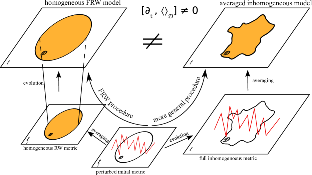
Figure 1: Illustration of the cause of the departure of the average evolution from the standard Friedmann solutions: the non–commutativity of spatial averaging and time–evolution. The standard Friedmannian picture is the left branch, where first the average over the inhomogeneous matter distribution is performed and the evolution of this homogeneous distribution is then evolved by the Einstein equations. In contrast to that, in the averaged model shown on the right branch, the evolution of the variables is calculated with the full metric and the average is taken over the evolved inhomogeneous distribution. The two approaches give in general different results. But the main question remains: How relevant is this difference?

Provenance of the averaged equations

In the recent literature, the question of how big the difference between these two approaches is, has received growing interest, mainly due to attempts to relate it to the volume acceleration (Dark Energy problem) buchert:jgrg , kolb:backreaction ,rasanen:de ; rasanen:acceleration ,buchert:review . Since then, there have been many calculations trying to quantify the impact of this non–commutativity of time–evolution and averaging. The direct way of trying to average the Einstein equations in their tensorial form is very involved, because it is not clear how to define a meaningful average of tensors. Therefore, a restriction to the averaging of scalar quantities is a way out of this problem and provides general features of the averaged dynamics buchert:dust ; buchert:fluid . In this approach, one uses the ADM equations to perform a $3+1$ split of the spacetime into spatial hypersurfaces orthogonal to the fluid flow. The source is also in this case often taken to be a perfect fluid and the equations take their simplest form in the frame of an observer comoving with the fluid. After this split one can identify scalar, vector and tensor parts of the resulting equations. For the scalar sector there is then a straightforward definition of an average quantity as the Riemannian volume integral of the scalar function, taken over a mass–preserving comoving domain of the spatial hypersurface, and divided by the volume of this domain. The use of this definition astonishingly provides a set of differential equations for the average scale factor of the averaging domain, that closely resembles the Friedmann equations in the homogeneous case:

$$3H_{\mathcal{D}}^{2}=8\pi G\left\langle\varrho\right\rangle_{\cal D}-\frac{1}{2}\left\langle\mathcal{R}\right\rangle_{\cal D}-\frac{1}{2}{\cal Q}_{\mathcal{D}}+\Lambda\;;$$

$$3\frac{\ddot{a}_{\mathcal{D}}}{a_{\mathcal{D}}}=-4\pi G\left\langle\varrho\right\rangle_{\cal D}+{\cal Q}_{\mathcal{D}}+\Lambda\;;$$

$$\langle\varrho{\dot{\rangle}}+3H_{\mathcal{D}}\left\langle\varrho\right\rangle_{\cal D}=0\;;\;a_{{\mathcal{D}}}^{-2}(a_{{\mathcal{D}}}^{2}{\mathcal{R}}_{\mathcal{D}}{\dot{)}}+a_{{\mathcal{D}}}^{-6}(a_{{\mathcal{D}}}^{6}{{\cal Q}}_{{\mathcal{D}}}{\dot{)}}=0.$$

This is surprising, because in this approach it is not necessary to constrain the matter source to a homogeneous–isotropic one, but one can have arbitrary spatial variations in the density and the geometrical variables. There are, however, two important differences between the general averaged evolution equations for the volume scale factor $a_{{\cal D}}\propto V_{{\cal D}}^{1/3}$ and the Friedmann equations. First, there is one extra term ${\cal Q}_{{\cal D}}$, which is called the kinematical backreaction term. It encodes the departure in the spatial hypersurface from a homogeneous distribution. It is defined as the variance of the local expansion rate of the spacetime minus the variance of the shear inside the domain ${\cal D}$. Therefore, if the expansion fluctuations are bigger than the shear fluctuations, ${\cal Q}_{{\cal D}}$ is positive and contributes to the acceleration of the spatial domain. For dominating shear fluctuations, ${\cal Q}_{{\cal D}}$ is negative and decelerates the domain’s expansion. This effective term ${\cal Q}_{{\cal D}}$, that emerges from the explicit averaging procedure, also induces the second difference to the standard Friedmann equations: an integrability condition assures that the expansion law is the integral of the acceleration law. While for the Friedmann equations this integrability is guaranteed through mass conservation, here there is a generalized conservation law that, besides mass conservation, dynamically links ${\cal Q}_{{\cal D}}$ to the average intrinsic curvature on the domain ${\cal D}$. Unlike in the Friedmann case, where the curvature scales as $a_{{\cal D}}^{-2}$, the dependence of the average curvature $\left\langle{\cal R}\right\rangle_{\cal D}$ on $a_{{\cal D}}$ has not necessarily the form of a simple power law. In fact it can be shown that the curvature picks up a time–integrated contribution along the history of the evolution of ${\cal Q}_{{\cal D}}$, and evolves in this way generically away from flat initial conditions, expected to emerge from inflation.

Uncommon properties of the averaged model

These two changes to the standard Friedmann equations may alter the expansion history considerably. Regarding Eqs. (2), it is easy to see that for ${\cal Q}_{{\cal D}}>4\pi G\left\langle\varrho\right\rangle_{\cal D}$ there may even be an accelerated epoch of expansion without the presence of a cosmological constant. It may seem surprising that even in a Universe filled with a perfect fluid of ordinary (or dark) matter only, there may be an effective acceleration of a spatial domain ${\cal D}$. This occurs, because in the calculation of the average expansion rate of ${\cal D}$, the deviations of the local expansion rates from the average introduce a positive–definite, non–local fluctuation term $\left\langle(\theta-\left\langle\theta\right\rangle_{\cal D})^{2}\right\rangle_{\cal D}$. Also, the average is weighted by its corresponding volume. Therefore, faster expanding subregions of ${\cal D}$, which will by their faster growth occupy a larger and larger volume fraction of ${\cal D}$, will eventually dominate the global expansion. Subregions whose expansion slows down will finally occupy a much smaller fraction of the volume of ${\cal D}$. This implies that a volume–weighted average of the expansion rate will start from a value between the one of the slow and fast expanding regions, when they have still a comparable size, but will be driven towards the value of the fastest expanding domains in the late–time limit. This growth in the average expansion rate corresponds to an acceleration of the volume scale factor.

A convenient way to illustrate the possible departure of the solutions of the equations for the average scale factor, from the Friedmann solution, is the phase space analysis of scaling solutions provided in morphon : the standard Einstein–de Sitter model is unstable, a saddle point in the enlarged class of solutions for averaged inhomogeneous models. Perturbations of the homogeneous state in the matter–dominated era will therefore drive the average properties of the Universe away from the standard model in the direction of an accelerated, expanding and almost–isotropic state. This is also the region in which the ${\cal Q}_{{\cal D}}$ term is positive. Therefore the instability of the Friedmann model leads naturally to accelerated expansion, if the phase space is traversed rapidly enough. A more elaborated phase space analysis may be found in Roy:Scale .

The important changes to the Friedmann model that emerge when passing to explicit averages, may be summarized in the following list of generalizing concepts:

1. The homogeneous and isotropic solution of Einstein’s equations is replaced by explicit averages of the equations of General Relativity.

2. The description is background–free, and inhomogeneities do no longer average out on a background.

3. The averaged model can be regarded as a generalized background that is generically interacting with structures in the spatial hypersurfaces.

4. The full Riemannian curvature degree of freedom is restored and the geometry no longer is restricted to a constant–curvature space.

A more detailed review of our current understanding of the description of the average evolution may be found in buchert:review ; rasanen:acceleration .

Partitioning models

To build a specific model using the above framework there have been several attempts. As the equations for $a_{{\cal D}}\left(t\right)$ are not closed, one has to impose, like in the Friedmann case, an equation of state for the fluid. The problem is here, that the fluid composed of backreaction ${\cal Q}_{{\cal D}}$ and average curvature $\left\langle{\cal R}\right\rangle_{\cal D}$ is only an effective one. Therefore it is not clear which equation of state one should choose, since it is dynamically determined by the inhomogeneities that are averaged over. In buchert:Chaplygin for example, the equation of state of a Chaplygin gas has been used. Another approach in morphon has been to take a constant equation of state that is popular in quintessence models. This leads to simple scaling solutions for the $a_{{\cal D}}$ dependence of ${\cal Q}_{{\cal D}}$ and $\left\langle{\cal R}\right\rangle_{\cal D}$. Those will be generalized here by the partitioning model, described in detail in wiegand .

Model construction

As the name suggests, our model implements a general partitioning of a domain of homogeneity ${\cal D}$ into subdomains buchertcarfora . To have a physical intuition about the evolution of the subdomains, a reasonable choice is to partition ${\cal D}$ into over–dense ${\cal M}$– and under–dense ${\cal E}$–regions. ${\cal M}$ and ${\cal E}$ regions will also obey the average equations (2) and there are consistency conditions, resulting from the split of the ${\cal D}$ equations into ${\cal M}$ and ${\cal E}$ equations, that link the evolution of ${\cal D}$, ${\cal M}$ and ${\cal E}$. The reason for the split is that it offers the possibility to replace the less accessible backreaction parameter ${\cal Q}_{{\cal D}}$ by a quantity that illustrates more directly the departure from homogeneity, namely the volume fraction of the over–dense regions $\lambda_{{\cal M}}$. As explained above, $\lambda_{{\cal M}}$ is expected to decrease during the evolution and it is this decrease that drives the acceleration. The physical motivation to split into over– and under–dense regions is that from the structure of the cosmic web one may expect ${\cal E}$ regions, which are mainly composed of voids, to be more spherical than ${\cal M}$ regions. On ${\cal E}$, the expansion fluctuations should therefore be larger than the shear fluctuations and so ${\cal Q}_{{\cal E}}$ should be positive. The shear fluctuation–dominated ${\cal M}$ regions should have a negative ${\cal Q}_{{\cal M}}$. This increases the difference between the faster expanding ${\cal E}$ and the decelerating ${\cal M}$ regions even further and therefore magnifies the expansion fluctuations on ${\cal D}$ that drive acceleration via a positive ${\cal Q}_{{\cal D}}$. The fact that ${\cal Q}_{{\cal M}}$ and ${\cal Q}_{{\cal E}}$ are nonzero is the main difference to a similar model of Wiltshire wiltshire:avsolution ; wiltshire:clocks .

The generalization of the single scaling laws mentioned above is achieved by imposing the scaling on ${\cal M}$ and on ${\cal E}$. In li:scale the authors showed that ${\cal Q}_{{\cal D}}$ and $\left\langle{\cal R}\right\rangle_{\cal D}$ may be expressed in a Laurent series starting at $a_{{\cal D}}^{-1}$ and $a_{{\cal D}}^{-2}$ respectively. This behavior breaks down if the fluctuations with respect to the mean density become of order one. This happens later on ${\cal M}$ as well as on ${\cal E}$, because on these regions the mean values lie above, respectively below the global mean, and therefore the fluctuations on ${\cal M}$ with respect to this over–dense mean are smaller than the variation between the peaks on ${\cal M}$ and the troughs on ${\cal E}$. Therefore, the $a_{{\cal D}}^{-1}$–scaling for ${\cal Q}_{{\cal D}}$ on ${\cal M}$ and ${\cal E}$ is expected to hold true even if the ${\cal D}$ regions already depart from this perturbatively determined behavior. The partitioning model is therefore the first step of a generalization to a physically justified nonlinear behavior of ${\cal Q}_{{\cal D}}$ and $\left\langle{\cal R}\right\rangle_{\cal D}$ on the global domain ${\cal D}$.

Using this ansatz for the ${\cal Q}_{{\cal D}}$-evolution on ${\cal M}$ and ${\cal E}$, and exploiting the consistency conditions for the partitioning, it is possible to arrive at a model that depends only on three parameters: the Hubble rate today $H_{{\cal D}_{0}}$, the matter density today $\Omega_{m}^{{\cal D}_{0}}$ and the volume fraction of the over–dense regions today $\lambda_{{\cal M}_{0}}$. In this parametrization $H_{{\cal D}_{0}}$ only sets the time scale, so that we may fix the evolution with $\Omega_{m}^{{\cal D}_{0}}$ and $\lambda_{{\cal M}_{0}}$. Assuming for $\Omega_{m}^{{\cal D}_{0}}$ the concordance value of $0.27$, the model shows that the more structure there is, indicated by a low value of $\lambda_{{\cal M}_{0}}$, the higher the acceleration on the domain ${\cal D}$ will be.

To analyze what the order of magnitude of $\lambda_{{\cal M}}$ is today, an N–body simulation was studied. Smoothing the point distribution on $5\mathrm{h^{-1}Mpc}$ and applying a simple number count for the determination of $\lambda_{{\cal M}_{0}}$, a value of $0.09$ was obtained. An analysis by a Voronoi tessellation gave about $0.02$. To obtain a definite value, this analysis clearly has to be improved. One would have to use a proper SPH smoothing and trace the Lagrangian regions, that are fixed in the initial conditions, until today. But in any case, $\lambda_{{\cal M}_{0}}$ seems to be in the region below $0.1$. Interestingly enough, this is the region for $\lambda_{{\cal M}_{0}}$ which leads to a nearly constant ${\cal Q}_{{\cal D}}$ on ${\cal D}$, shown in Fig. 2. Hence, for low values of $\lambda_{{\cal M}_{0}}$, ${\cal Q}_{{\cal D}}$ acts like a cosmological constant.

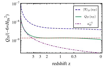
Figure 2: Evolution of the backreaction parameter ${\cal Q}_{{\cal D}}$ in the course of cosmic time. From a value of $\Omega_{{\cal Q}}^{{\cal D}}$ of around $10^{-7}$ at a redshift of $z\approx 1000$, ${\cal Q}_{{\cal D}}$ first decreases like $a_{{\cal D}}^{-1}$ and becomes approximately constant for a long period of the evolution when $\dot{\lambda}_{{\cal M}}$ gets important.

Observational strategies

This may also be seen by a fit of the model to luminosity distances of supernovae (SN). To convert the evolution of the average scale factor $a_{{\cal D}}$ into luminosity distances, we use the result of Räsänen rasanen:light , who investigated the propagation of light in inhomogeneous universe models and provided a formula linking the observed luminosity distance to the volume scale factor $a_{{\cal D}}$. The resulting probability contours in the parameter space $\Omega_{m}^{{\cal D}_{0}}$–$\lambda_{{\cal M}_{0}}$ in Fig. 3 show, that indeed the region around an $\Omega_{m}^{{\cal D}_{0}}$ of $0.3$ and a $\lambda_{{\cal M}_{0}}$ below $0.1$ is favored by the data.

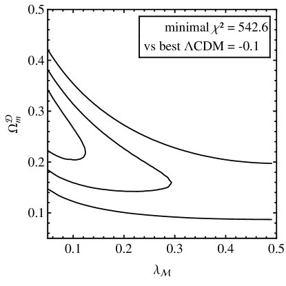
Figure 3: Probability contours of a fit [Martin Kunz priv. comm.] of the partitioning model to the Union2 SN data set. The model gives a comparably reasonable fit as a simple $\Lambda$CDM model.

To further test the viability of the model, it will soon be compared with more observational data. But as it is probably possible to fit also these, as indicated by the success of morphon:obs , we need a quantity that will definitively allow to find out whether this model or one with a real cosmological constant fits better. To decide that, one may use a quantity introduced by Clarkson clarkson , namely the $C$–function

$$C\left(z\right)=1+H^{2}\left(DD^{\prime\prime}-D^{\prime 2}\right)+HH^{\prime}DD^{\prime}\;.$$ (3)

It consists of derivatives of the Hubble rate $H\left(z\right)$ and the angular diameter distance $D\left(z\right)$, and is constructed such that for every FRW model it is exactly 0 for any $z$. For the partitioning model this is generically not the case and for several choices of parameters the difference is shown in Fig. 4 using the template metric of morphon:obs . Unfortunately, the function $C\left(z\right)$ is too complicated to evaluate it using present–day data, but as shown in morphon:obs , the EUCLID mission may be able to derive its values.

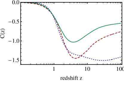
Figure 4: Plot of Clarkson’s C–function for several models discussed in wiegand . The model presented here is shown as the dotted line. The dashed line is its non–perturbative generalization explained in wiegand , and the solid line is a single scaling model. For every Friedmann model $C\left(z\right)\equiv 0$, which allows to distinguish averaged models from FRW models.

Conclusion

Routing the accelerated expansion back to inhomogeneities furnishes an interesting possibility to avoid problems with a cosmological constant, such as the coincidence problem and would give the sources of acceleration a physical meaning. If perturbations are analyzed on a fixed FRW background it is clear that the effect is way to small to give rise to an acceleration on the scale of the Hubble volume (brown1 ; brown2 ). There are, however, semi–realistic non–perturbative models rasanen:peakmodel that show that a considerable effect is not excluded. Furthermore it has been shown why perturbative models are not able to give a definite answer on the magnitude of the effect rasanen:FRW , buchert:review . It seems that the question of how the growth of structure influences the overall expansion of the Universe is still an open issue. The presented partitioning model can demonstrate that a $\Lambda$CDM–like expansion is possible in the context of these models, without the prior assumption of ${\cal Q}_{{\cal D}}=const.$, which emerges here more naturally. Furthermore it has been shown how this is related to the formation of structure described by the parameter $\lambda_{{\cal M}}$. Finally, using Clarkson’s C–function, we will have, at the latest with the data from the EUCLID mission, a handle on how to distinguish acceleration due to inhomogeneities from acceleration due to the presence of a strange fluid. All in all, these are promising prospects for the future.

Acknowledgments: We would like to thank Christian Byrnes and Dominik J. Schwarz for useful comments on the manuscript. This work is supported by DFG under Grant No. GRK 881.

References

- (1) I.A. Brown, J. Behrend and K.A. Malik: Gauges and cosmological backreaction. JCAP 11, 027 (2009)
- (2) I.A. Brown, G. Robbers and J. Behrend: Averaging Robertson–Walker cosmologies. JCAP 4, 016 (2009)
- (3) T. Buchert: On average properties of inhomogeneous fluids in general relativity: dust cosmologies. Gen. Rel. Grav. 32, 105 (2000)
- (4) T. Buchert: On average properties of inhomogeneous fluids in general relativity: perfect fluid cosmologies. Gen. Rel. Grav. 33, 1381 (2001)
- (5) T. Buchert: On average properties of inhomogeneous cosmologies. In: 9th JGRG Meeting, Hiroshima 1999, Y. Eriguchi et al. (eds.), J.G.R.G. 9, 306–321 (2000), arXiv:gr–qc/0001056
- (6) T. Buchert: Dark Energy from structure – a status report. Gen. Rel. Grav. 40, 467 (2008).
- (7) T. Buchert, J. Larena and J.–M. Alimi: Correspondence between kinematical backreaction and scalar field cosmologies – the ’morphon field’. Class. Quant. Grav. 23, 6379 (2006)
- (8) T. Buchert and M. Carfora: On the curvature of the present–day Universe. Class. Quant. Grav. 25, 195001 (2008)
- (9) C. Clarkson, B. A. Basset and T. Hui–Ching Lu: A general test of the Copernican Principle. Phys. Rev. Lett. 101 011301 (2008)
- (10) G.F.R. Ellis: Relativistic cosmology: its nature, aims and problems. In General Relativity and Gravitation (D. Reidel Publishing Company, Dordrecht, 1984), pp. 215–288
- (11) G.F.R. Ellis and T. Buchert: The Universe seen at different scales. Phys. Lett. A (Einstein Special Issue) 347, 38 (2005)
- (12) E.W. Kolb, S. Matarrese, A. Notari and A. Riotto: Effect of inhomogeneities on the expansion rate of the Universe. Phys. Rev. D 71, 023524 (2005)
- (13) J. Larena, J.–M. Alimi, T. Buchert, M. Kunz and P.–S. Corasaniti: Testing backreaction effects with observations. Phys. Rev. D 79, 083011 (2009)
- (14) N. Li and D. J. Schwarz: Scale dependence of cosmological backreaction. Phys. Rev. D 78, 083531 (2008)
- (15) S. Räsänen: Dark energy from backreaction. JCAP 2, 003 (2004)
- (16) S. Räsänen: Accelerated expansion from structure formation. JCAP 11, 003 (2006)
- (17) S. Räsänen: Evaluating backreaction with the peak model of structure formation. JCAP 4, 026 (2008)
- (18) S. Räsänen: Light propagation in statistically homogeneous and isotropic dust universes. JCAP 2, 011 (2009)
- (19) S. Räsänen: Applicability of the linearly perturbed FRW metric and Newtonian cosmology. Phys. Rev. D 81 103512 (2010)
- (20) X. Roy and T. Buchert: Chaplygin gas and effective description of inhomogeneous universe models in general relativity. Class. Quant. Grav. 27 175013 (2010)
- (21) X. Roy, T. Buchert, S. Carloni and N. Obadia: Global gravitational instability of FLRW backgrounds: dynamical system analysis of the dark sectors. arXiv:1103.1146 (2011)
- (22) M.F. Shirokov and I.Z. Fisher, Sov. Astron. J. 6, 699 (1963); reprinted in Gen. Rel. Grav. 30, 1411 (1998).
- (23) A. Wiegand and T. Buchert: Multiscale cosmology and structure–emerging Dark Energy: A plausibility analysis. Phys. Rev. D 82 023523 (2010)
- (24) D. L. Wiltshire: Cosmic clocks, cosmic variance and cosmic averages. NJP 9, 377 (2007)
- (25) D. L. Wiltshire: Exact solution to the averaging problem in cosmology. Phys. Rev. Lett. 25, 251101 (2007)