The Hagedorn Temperature Revisited.

Abstract

The Hagedorn temperature, $T_{H}$ is determined from the number of hadronic resonances including all mesons and baryons. This leads to a stable result $T_{H}=174$ MeV consistent with the critical and the chemical freeze-out temperatures at zero chemical potential. We use this result to calculate the speed of sound and other thermodynamic quantities in the resonance hadron gas model for a wide range of baryon chemical potentials following the chemical freeze-out curve. We compare some of our results to those obtained previously in other papers.

25.75,-q.05.70,-a,64.70,-p,64.90,+b

1 Introduction

In 1965 Hagedorn  [1] proposed that the number of hadronic resonances increases exponentially with the mass $m$ of the resonances. The idea, which was debated strongly when first proposed, has since been widely accepted and discussed by many authors [2, 3, 4, 5, 6, 7, 8, 9, 10, 11]. The concept was based on the assumption that the observed increase in the number of hadronic resonances would continue towards higher and higher masses as more experimental data became available [12]. The scale of the exponential increase determines the value of the Hagedorn temperature, $T_{H}$. Recent papers  [13, 14, 15, 16, 17, 18] have used the latest results from the Particle Data Group [12] to revisit the original analysis of Hagedorn to update the value of $T_{H}$. This resulted in a surprising wide spread of possible values, with large variations as to whether one considers mesons or baryons with values ranging from $T_{H}=141$ MeV to $T_{H}=340$ MeV depending on the parametrization used and on the set of hadrons (mesons or baryons). There thus exists uncertainty as to the value of the Hagedorn temperature. These have two origins:

• sparse information about hadronic resonances certainly above 3 GeV,

• the analytical form of the Hagedorn spectrum, especially the factor multiplying the exponential.

The first item will probably never be resolved satisfactorily due to the width of resonances and also due to their large number making it difficult to identify them. Splitting the spectrum into baryons and mesons further decreases the quality of the fits to the mass dependence of the mass spectrum. We therefore propose to stick to the original analysis of Hagedorn and consider a sum over all resonances, baryons, mesons, strange, non-strange, charm, bottom etc.. This is the state that is produced at the Large Hadron Collider (LHC), namely, a hadronic ensemble containing all possible resonances. The result is shown in Fig. 1 and leads to a good determination of $T_{H}$ because the range in $m$ is reasonably large extending up to 3 GeV before reaching a plateau presumably due to the parsity of hadronic resonances above this value. Details about the parametrization used will be presented below.

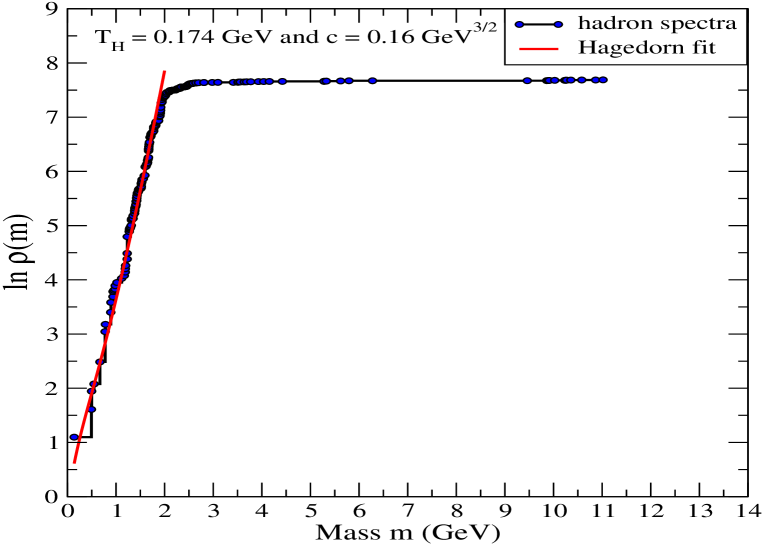
Figure 1: Cumulative number of hadronic resonances as a function of $m$. Again the hadronic data are made up of all resonances, including baryons, mesons and also heavy resonances made up of charm and bottom quarks.

The Hagedorn temperature naturally leads to the notion that hadronic matter cannot exceed a limiting temperature and increasing the beam energy in proton$-$proton and proton$-$antiproton̄ collisions results in more and more hadronic resonances being produced without a corresponding increase in the temperature of the final (freeze-out) state. This is the situation observed at the highest energies at the LHC. It was suggested long ago [3] that the Hagedorn temperature is connected to the existence of a different phase in which quarks and gluons are no longer confined. At present, the Hagedorn temperature is often understood as the temperature of the phase transition from hadrons to a quark-gluon plasma.
A recent analysis [15, 24] investigated the hadron resonance gas model [19, 20, 21] to show the stability of various thermodynamic quantities in heavy-ion collisions when the Hagedorn spectrum is used literally, i.e. without a cut-off on the number of resonances beyond a certain mass. In particular, the authors explored the addition of the hadron resonance gas model including an exponentially large number of undiscovered resonances which are naturally included in the Hagedorn model. Their results showed that the hadron resonance gas model gave different results for thermodynamic quantities but the overall chemical analysis was reasonably stable.

Furthermore, the use of so-called Hagedorn States (HS), based on the exponentially increasing spectrum, close to the critical temperature can explain fast chemical equilibration by HS regeneration [22] and provide a unique method to compare lattice results for $T_{c}$ using thermal fits HS provide a lower $\chi^{2}$ than thermal fits without HS [23]. These authors estimated effects by extending the hadron mass spectrum beyond $3$ GeV for $T_{H}$ = 200 MeV and assume that high mass excited $K^{*}$ states produce one kaon while producing multiple pions thus further reducing the $K^{+}/\pi^{+}$ [24].

In this paper, we extend previous work [25, 26, 27] by extending explicit expressions of relevant thermodynamic quantities for non-zero chemical potentials. In particular the speed of sound, $C_{s}^{2}$, can be considered as a sensitive indicator of the critical behavior in strongly interacting matter. The results show a sharp dip of $C_{s}^{2}$ in the critical region, which is an indication that thermodynamics in the vicinity of confinement is indeed driven by the higher excited hadronic states.
The outline of this paper is as follows. In section 2, we present the influence of the Hagedorn spectrum on the hadron yields to find the thermodynamic parameters and explain the basic concepts used in this paper. In section 3, we derive the number, energy and entropy densities and also the speed of sound. In section 4, we show the results using the hadron and its extension resonance gas model for particular thermodynamic quantities and discuss the relationship of $C_{s}^{2}$ with temperature and chemical potentials and compare thermodynamic quantities, like energy and entropy density. The last section covers the conclusion.

2 Motivation

The particle data table contains hundreds of hadronic resonances [12] including the well known stable hadrons like nucleons, pions, hyperons ($\omega$, $\Sigma$, $\Xi$), kaons etc.. In our calculations we used a list of hadronic resonances including in total $250$ baryons and antibaryons, $348$ mesons and antimesons (counted without considering their isospin and spin degeneracies). Most of the hadronic resonances decay quickly via strong interactions before reaching the detector, hence they are usually identified via their decay products. The mass of a decaying particle is equal to the total energy of the products measured in its rest frame.
The basic idea of this paper is to add resonances using the Hagedorn model for the spectrum. Using the hadronic data we show the relationship between the number of hadronic resonances and the mass in Fig. 1 where we took hadrons with masses up to $11.019$ GeV. The density of states obtained this way has been fitted using the following equation [2];

$$\rho_{h}(m)=\frac{c}{\left(m^{2}+m_{0}^{2}\right)^{5/4}}\exp{\left(\frac{m}{T_{H}}\right)},$$ (1)

where $c$ and $m_{0}$ are constant parameters given in the table below

Parameter
$c$ $(GeV)^{3/2}$	0.16 $\pm$ 0.02
$m_{0}$ $(GeV)$	0.5
$T_{H}$ $(GeV)$	0.174 $\pm$ 0.011

Table 1: The result for the parameters of $c$, $m_{0}$ and $T_{H}$ using equation $(1)$.

3 The Hadron Resonance Gas Model and its Extension

The thermodynamic properties of the Hadron Resonance Gas Model (HRGM) can be determined from the partition function

$$\ln Z(V,T,\mu) = \int dm\left[\rho_{M}(m)\ln Z_{b}(m,V,T,\mu)\right.$$ (2)

$$\left.+\hskip 8.5359pt\rho_{B}(m)\ln Z_{f}(m,V,T,\mu)\right],$$

where the gas is contained in a volume $V$, has a temperature $T$ and chemical potential $\mu$, $Z_{b}$ and $Z_{f}$ are the partition functions for an ideal gas of bosons and fermions respectively with mass $m$, $\rho_{M}(m)$ and $\rho_{B}(m)$ are the spectral density of mesons and baryons. By using Eq. 2, one can compute the number denisty $n$, energy density $\varepsilon$, entropy density $s$, pressure $P$, speed of sound $C_{s}^{2}$ and specific heat $C_{v}$.
hadron properties enter these models through $\rho_{M,B}$. The HRGM model takes the observed spectrum of hadrons up to some cutoff of mass $\lambda$, defined by

$$\rho_{M,B}(m)=\sum_{i}^{m_{i}\leq\lambda}g_{i}\delta(m-m_{i}),$$ (3)

where $m_{i}$ are the masses of the known hadrons and $g_{i}$ the degeneracy factor. In order to explore the stability of results obtained using the HRGM, variant of these models is often used in which one takes the observed spectrum of states up to a certain cutoff of mass $\lambda$ and above this one includes an exponentially rising cumulative density of hadron states, which is defined in Eq. 1. This defines the Extended Hadron Resonance Gas Model (EHRGM). The density of states becomes

$$\rho_{h}(m)=\sum_{i}^{m_{i}\leq\lambda}g_{i}\delta(m-m_{i})+\frac{c}{(m^{2}+m_{0}^{2})^{5/4}}\exp{\left(\frac{m}{T_{H}}\right)}\theta(m-\lambda),$$ (4)

where the model parameter $c$ and $T_{H}$ are fitted to data on the cumulative distribution of the sets of hadrons, $h$. Typically this model uses $m_{0}=$ $0.5$ GeV. Moreover, the parameters are determined from the hadronic spectrum with masses up to $3$ GeV as shown in Fig. 1. The results for $c$ and $T_{H}$ are given in Table 1.

4 Derivation of thermodynamic quantities in EHRGM

We are considering here the Boltzmann distribution for simplicity in order to present some of the results in a compact form. The partition function for a single particle is given by

$$\ln Z=\frac{gVTm^{2}}{2\pi^{2}}K_{2}\left(\frac{m}{T}\right)\exp{\left(\frac{\mu}{T}\right)},$$ (5)

where $K_{2}$ is modified Bessel function. The meson mass distribution is taken to be given by

$$\rho_{M,B}(m)=\sum_{i=1}^{m_{i}<\lambda}g_{i}^{M,B}\delta(m-m_{i})+\frac{c}{(m^{2}+m_{0}^{2})^{5/4}}\exp{\left(\frac{m}{T_{H}}\right)}\theta(m-\lambda),$$ (6)

4.1 Derivation for the particle densities and pressure

The particle density can be written as the sum of the two terms

$$n=n_{M}+n_{B},$$ (7)

where $n_{M}=\ln Z_{M}/V$ and $n_{B}=\ln Z_{B}/V$ are number densities of mesons and baryons respectively. They are defined by

$$n_{M,B} = \frac{T}{2\pi^{2}}\sum_{i=1}^{m_{i}<\lambda}\exp{\left(\frac{\mu_{i}}{T}\right)}\left[g_{i}^{M,B}m_{i}^{2}K_{2}\left(\frac{m_{i}}{T}\right)\hskip 8.5359pt+\right.$$ (8)

$$\left.c\int_{m=\lambda}^{\infty}\frac{m^{2}}{(m^{2}+m_{0}^{2})^{5/4}}\exp{\left(\frac{m}{T_{H}}\right)}K_{2}\left(\frac{m}{T}\right)dm\right],$$

where $\mu_{i}=S_{i}\mu_{S}+B_{i}\mu_{B}+Q_{i}\mu_{Q}$, for our case we consider an isospin symmetric system, where $\mu_{Q}=$ $0.0$ GeV. The pressure is given by

$$P=T\frac{\partial\ln Z_{M}}{\partial V}+T\frac{\partial\ln Z_{B}}{\partial V}=P_{M}+P_{B},$$ (9)

where $P_{M}=Tn_{M}$ and $P_{B}=Tn_{B}$ are the pressure of mesons and baryons respectively.

4.2 Derivation for energy density

The energy density is given by

$$\varepsilon_{M,B}=\frac{T^{2}}{V}\frac{\partial\ln Z_{M,B}}{\partial T},$$ (10)

where $K_{1}$ is the modified Bessel function, $\varepsilon_{M}$ and $\varepsilon_{B}$ are energy densities of mesons and baryons respectively.

$$\varepsilon_{M,B}=\sum_{i=1}^{m<\lambda}\left[\frac{T^{2}}{2\pi^{2}}\exp{\left(\frac{\mu_{i}}{T}\right)}\left(g_{i}^{M,B}m_{i}^{2}\left[3K_{2}\left(\frac{m_{i}}{T}\right)+\frac{m_{i}}{T}K_{1}\left(\frac{m_{i}}{T}\right)\right]+A_{H}\right)\right],$$ (11)

where

$$A_{H}=c\int_{m}^{\infty}\frac{m^{2}}{(m^{2}+m_{0}^{2})^{5/4}}\exp{\left(\frac{m}{T_{H}}\right)}K_{2}(\frac{m}{T})dm.$$

From the above expressions, we can obtain the entropy density

$$s=\frac{\varepsilon+P-n_{S}\mu_{S}-n_{B}\mu_{B}}{T},$$ (12)

where $n_{S}$ and $n_{B}$ are the net number densities for strange and baryonic particles respectively

$$n_{S(B)}=\frac{T}{V}\frac{\partial\ln Z}{\partial\mu_{S(B)}}.$$ (13)

4.3 Derivation of the speed of sound

In hydrodynamic models the speed of sound plays an important role in the evolution of a system and is an ingredient in the understanding of the effects of a phase transition [25, 26, 27, 28]. It is well-known [29] that the speed of sound has to be calculated at constant entropy per particle $(s/n)$. This makes the calculation more complicated than the one at zero chemical potential where it is sufficient to keep the temperature fixed. In our extension we take the condition [29] into account for non-zero baryon and strangeness chemical potentials, imposing overall strangeness zero. The squared speed is thus calculated starting from

$$C_{s}^{2}(T,\mu)=\left(\frac{\partial P}{\partial\varepsilon}\right)_{s/n},$$ (14)

The complete expression for the speed of sound can be rewritten as

$$C_{s}^{2}(T,\mu)=\frac{\left(\frac{\partial P}{\partial T}\right)+\left(\frac{\partial P}{\partial\mu_{S}}\right)\left(\frac{d\mu_{S}}{dT}\right)+\left(\frac{\partial P}{\partial\mu_{B}}\right)\left(\frac{d\mu_{B}}{dT}\right)}{\left(\frac{\partial\varepsilon}{\partial T}\right)+\left(\frac{\partial\varepsilon}{\partial\mu_{S}}\right)\left(\frac{d\mu_{S}}{dT}\right)+\left(\frac{\partial\varepsilon}{\partial\mu_{B}}\right)\left(\frac{d\mu_{B}}{dT}\right)},$$ (15)

where the derivatives $\frac{d\mu_{B}}{dT}$ and $\frac{d\mu_{S}}{dT}$ can be evaluated from two conditions. The first condition comes from the requirement that the ratio $(s/n)$ must be kept fixed,

$$\frac{s}{n}=0,$$ (16)

while the second condition follows from the conservation of strangeness

$$n_{S}=n_{\bar{S}}.$$ (17)

The resulting expressions for $\frac{d\mu_{B}}{dT}$ and $\frac{d\mu_{S}}{dT}$ are presented in detail in the appendix.

5 Results using HRGM and EHRGM

There is not much difference between the HRGM and EHRGM models at low temperature, $T\ll T_{H}$ since the heavy resonances do not play an important role there. Alternatively, at high temperatures, $T\gg T_{H}$, it should agree with the results of the lattice simulations of QCD [30, 31, 32]. In our case, we have determined the temperature and chemical potential dependencies of the pressure and the number, energy and entropy densities using the chemical freeze-out curve [19, 20, 21]. Using these results, we have then calculated the speed of sound. The thermodynamic variables obtained using HRGM, we plot the energy and entropy densities scaled by the appropriate powers of $T$, which is shown in Fig. 2a,  3a and  4a, at the $T_{H}=0.174$ GeV didn’t observe any sudden change of the thermodynamic variables $\varepsilon/T^{4}$ and $s/T^{3}$ close to the critical temperature, it showed smooth shape as the temperature goes beyong $T_{H}$.
Moreover, when we use the EHRGM, we see a different behaviour at the critical temperature which is shown in Fig. 2b,  3b and  4b. These show that if the system undergoes a first-order phase transition, both temperature and pressure remain constant as hadronic matter is converted from hadron gas to quark-gluon plasma; the energy and entropy density, however, change discontinuously. This leads to show us a new state of matter.

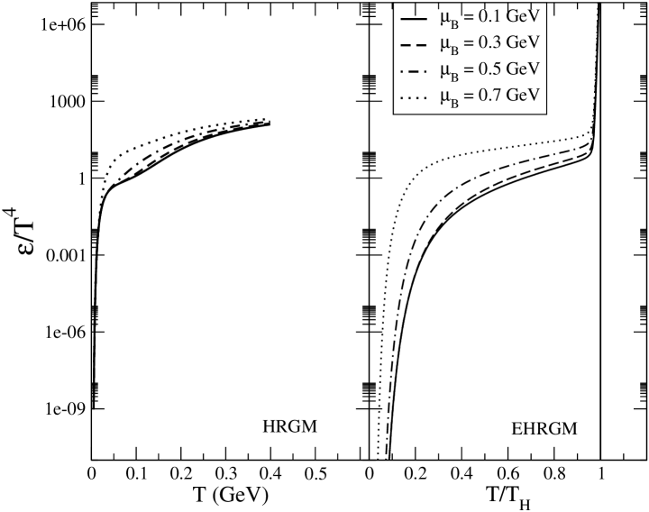
Figure 2: (a) This figure show that the energy density $\varepsilon$ in units of $T^{4}$ calculated on the HRGM as a function of the temperature $T$. (b) This figure show that the energy density $\varepsilon$ in units of $T^{4}$ for EHRGM as a function of the $T$. The full$-$lines are the result of the EHRGM that accounts for all mesonic and baryonic resonances.

Figure 3: (a)This figure show that the entropy $s$ in units of $T^{3}$ calculated in the HRGM as a function of the $T$. (b) Entropy $s$ in units of $T^{3}$ using EHRGM as a function of the $T$. The full$-$lines are the result of the EHRGM that accounts for all mesonic and baryonic resonances.

The value of the speed of sound remains well below the ideal-gas limit for massless particles $C_{s}^{2}=1/3$, even at very high temperatures, energy densities and pressure. In Fig. 4b represents, when it crosses the transition point in the case of full QCD, we expect as before that $C_{s}^{2}$ should vanish beside that $C_{s}^{2}$ is inversely proportional to the specific heat $C_{v}$, and this can lead to a divergence at the critical temperature $T_{c}$. Of course, due to finite volume effects, the velocity of sound will most likely not completely vanishes at $T=T_{c}$.

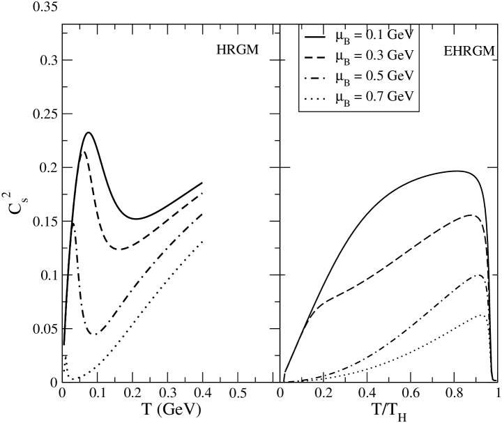
Figure 4: (a) Showing the speed of sound $C^{2}_{s}(T,\mu)$ calculated on the HRGM as a function of the $T$ and $\mu$. (b) The speed of sound $C^{2}_{s}(T,\mu)$ in EHRGM with resonance mass truncation, $m<$ 2 GeV

The velocity of sound versus the temperature as shown in Fig. 4b is to evaluate $dP/d\varepsilon$, we have followed [28] and first expressed $P$ and $\varepsilon$ in physical units, using EHRGM in Eq. 4. The temperature and chemical potential dependence of all the relevant thermodynamic quantities shows unique behaviour at the critical point $T_{c}$, specially for the speed of sound, there is a pronounced dip as evidence for the phase transition in the system. Based on our calculations, the velocity of sound at $T=T_{c}$ is different from zero; it is expected to become zero but due to finite volume effects.

6 Conclusions

In this paper we have made a new analysis of the number of hadronic resonances using the latest information from the Particle Data Group [12]. This leads to a temperature which is consistent with the most recent results based on lattice QCD estimates of the phase transition temperature [30, 31] and also the chemical freeze-out temperature at zero baryon density [19, 20, 21]. We have extended calculations of the speed of sound to non-zero baryon and strangeness chemical potentials keeping $s/n$ fixed [29]. This is done for both the hadronic resonance gas model (HRGM) and the extended hadronic resonance gas model (EHRGM) which includes the exponentially increasing spectrum of hadrons following the Hagedorn parametrization. The EHRGM shows that the speed of sound goes to zero at the phase transition point while the HRGM shows a smooth dip followed by an increase.

Appendix A Appendix: Speed of sound at non-zero chemical potentials.

The speed of sound is given by [29]

$$C_{s}^{2}(T,\mu)=\left(\frac{\partial P}{\partial\varepsilon}\right)_{\frac{s}{n}},$$ (18)

where $s/n$ is the entropy per particle which is kept fixed. using the variables $T,\mu_{B}$ and $\mu_{S}$, this can be rewritten as

$$C_{s}^{2}(T,\mu)=\frac{\left(\frac{\partial P}{\partial T}\right)+\left(\frac{\partial P}{\partial\mu_{S}}\right)\left(\frac{d\mu_{S}}{dT}\right)+\left(\frac{\partial P}{\partial\mu_{B}}\right)\left(\frac{d\mu_{B}}{dT}\right)}{\left(\frac{\partial\varepsilon}{\partial T}\right)+\left(\frac{\partial\varepsilon}{\partial\mu_{S}}\right)\left(\frac{d\mu_{S}}{dT}\right)+\left(\frac{\partial\varepsilon}{\partial\mu_{B}}\right)\left(\frac{d\mu_{B}}{dT}\right)},$$ (19)

where the derivatives $\frac{d\mu_{B}}{dT}$ and $\frac{d\mu_{S}}{dT}$ can be evaluated using two conditions. The first condition comes from keeping the ratio $(s/n)$ constant. From the derivative one obtains

$$d\left(\frac{s}{n}\right)=0,$$ (20)

which implies

$$nds=sdn.$$ (21)

In terms of $T$, $\mu_{B}$ and $\mu_{S}$ this equation can be written as

$$n\left(\frac{\partial s}{\partial T}\right)dT + n\left(\frac{\partial s}{\partial\mu_{B}}\right)d\mu_{B}+n\left(\frac{\partial s}{\partial\mu_{S}}\right)d\mu_{S}$$ (22)

$$= s\left(\frac{\partial n}{\partial T}\right)dT+s\left(\frac{\partial n}{\partial\mu_{B}}\right)d\mu_{B}+s\left(\frac{\partial n}{\partial\mu_{S}}\right)d\mu_{S}.$$

divide the above expression by $dT$ on both sides, so that it becomes

$$n\left(\frac{\partial s}{\partial T}\right) + n\left(\frac{\partial s}{\partial\mu_{B}}\right)\left(\frac{d\mu_{B}}{dT}\right)+n\left(\frac{\partial s}{\partial\mu_{S}}\right)\left(\frac{d\mu_{S}}{dT}\right)$$ (23)

$$= s\left(\frac{\partial n}{\partial T}\right)+s\left(\frac{\partial n}{\partial\mu_{B}}\right)\left(\frac{d\mu_{B}}{dT}\right)+s\left(\frac{\partial n}{\partial\mu_{S}}\right)\left(\frac{d\mu_{S}}{dT}\right).$$

Rearranging the above expression in order to write $\frac{d\mu_{B}}{dT}$ in terms of $\frac{d\mu_{S}}{dT}$ one obtains

$$\left[n\left(\frac{\partial s}{\partial\mu_{B}}\right)-s\left(\frac{\partial n}{\partial\mu_{B}}\right)\right]\left(\frac{d\mu_{B}}{dT}\right)$$

$$=s\left(\frac{\partial n}{\partial T}\right)-n\left(\frac{\partial s}{\partial T}\right)-\left[n\left(\frac{\partial s}{\partial\mu_{S}}\right)-s\left(\frac{\partial n}{\partial\mu_{S}}\right)\right]\left(\frac{d\mu_{S}}{dT}\right).$$ (24)

Defining

$$A = n\left(\frac{\partial s}{\partial T}\right)-s\left(\frac{\partial n}{\partial T}\right),$$ (25)

$$B = n\left(\frac{\partial s}{\partial\mu_{B}}\right)-s\left(\frac{\partial n}{\partial\mu_{B}}\right),$$ (26)

$$C = n\left(\frac{\partial s}{\partial\mu_{S}}\right)-s\left(\frac{\partial n}{\partial\mu_{S}}\right).$$ (27)

The final expression for condition one is

$$\frac{d\mu_{B}}{dT}=-\frac{1}{B}\left[A+C\frac{d\mu_{S}}{dT}\right].$$ (28)

The second condition comes from overall strangeness neutrality, which is

$$n_{S}=n_{\bar{S}}$$ (29)

where $n_{S}$ and $n_{\bar{S}}$ are the strange and antistrange particle densities. Similarly the derivative of equation Eq. 29 should thus satisfy

$$d(n_{S})=d(n_{\bar{S}})$$ (30)

this implies equation Eq. 30 can be expressed as

$$\left(\frac{\partial n_{S}}{\partial T}\right)+\left(\frac{\partial n_{S}}{\partial\mu_{B}}\right)\left(\frac{d\mu_{B}}{dT}\right)+\left(\frac{\partial n_{S}}{\partial\mu_{S}}\right)\left(\frac{d\mu_{S}}{dT}\right)$$

$$=\left(\frac{\partial n_{\bar{S}}}{\partial T}\right)+\left(\frac{\partial n_{\bar{S}}}{\partial\mu_{B}}\right)\left(\frac{d\mu_{B}}{dT}\right)+\left(\frac{\partial n_{\bar{S}}}{\partial\mu_{S}}\right)\left(\frac{d\mu_{S}}{dT}\right).$$ (31)

We can apply the same method as above to write $\frac{d\mu_{B}}{dT}$ in terms of $\frac{d\mu_{S}}{dT}$ for the above relation

$$\left[\left(\frac{\partial n_{S}}{\partial\mu_{B}}\right)-\left(\frac{\partial n_{\bar{S}}}{\partial\mu_{B}}\right)\right]\left(\frac{d\mu_{B}}{dT}\right)$$ (32)

$$= \left(\frac{\partial n_{\bar{S}}}{\partial T}\right)-\left(\frac{\partial n_{S}}{\partial T}\right)-\left[\left(\frac{\partial n_{S}}{\partial\mu_{S}}\right)-\left(\frac{\partial n_{\bar{S}}}{\partial\mu_{S}}\right)\right]\left(\frac{d\mu_{S}}{dT}\right),$$

we define $L=n_{S}$, hence it represents that the number of strangeness density for baryons and mesons

$$L=n_{S}^{B}+n_{S}^{M},$$

and $R=n_{\bar{S}}$, the number of antistrangeness density for baryons and mesons

$$R=n_{S}^{\bar{B}}+n_{S}^{\bar{M}}.$$

Define now

$$E = \frac{\partial L}{\partial\mu_{B}}-\frac{\partial R}{\partial\mu_{B}},$$ (33)

$$F = \frac{\partial L}{\partial\mu_{S}}-\frac{\partial R}{\partial\mu_{S}},$$ (34)

$$D = \frac{\partial L}{\partial T}-\frac{\partial R}{\partial T}.$$ (35)

Hence, the final expression for condition two becomes

$$\frac{d\mu_{B}}{dT}=-\frac{1}{E}\left[D+F\frac{d\mu_{S}}{dT}\right].$$ (36)

Finally, by equating equation  28 and  36 we find

$$\frac{d\mu_{S}}{dT}=\frac{AE-BD}{BF-CE},$$ (37)

and

$$\frac{d\mu_{B}}{dT}=\frac{CD-AF}{BF-CE},$$ (38)

Which is the relation used in the text.

References

References

- [1] R. Hagedorn, Supplemento al Nuovo Cimento Volume III, 147 (1965); Nuovo Cimento 35 (1965) 395; Nuovo Cimento 56 A (1968) 1027.
- [2] R. Hagedorn and J. Ranft, Nucl. Phys. B 48 (1972) 157-190.
- [3] N. Cabibbo and G. Parisi, Phys. Lett. B 59 (1975) 67.
- [4] G. Veneziano, Nuovo Cimento 57A (1968) 190.
-
[5]
K. Bardakci and S. Mandelstam, Phys. Rep.184 (1969) 1640;
S. Fubini and G. Veneziano, Nuovo Cimento 64A (1969) 811. - [6] K. Huang and S. Weinberg, Phys. Rev. Lett. 25 (1970) 895.
- [7] H. Satz, Phys. Rev. D 19 (1979) 1912.
- [8] Ph. Blanchard, S. Fortunato and H. Satz, Eur. Phys. J. C 34 (2004) 361.
- [9] R. V. Gavai and A. Goksch, Phys. Rev. D 33 (1986) 614.
- [10] K. Redlich and H. Satz, Phys. Rev. D 33 (1986) 3747.
- [11] F. Karsch, E. Laermann and A. Peikert, Phys. Lett. B 478 (2000) 447.
- [12] Particle Data Group, C. Caso et al., Eur. Phys. J. C 3, (1998) 1-794
- [13] M. Chojnacki, W. Florkowski and T. Csorgo, Phys. Rev. C 71 (2006) 044902.
- [14] M. Chojnacki and W. Florkowski Acta Physica Polonica B 38 (2007) 3249.
- [15] S. Chatterjee, S. Gupta and R. M. Godbole, Phys. Rev. C 81 044907 (2010).
- [16] W. Broniowski, W. Florkowski and L. Y. Glozman, Phys. Rev. D 70 (2004) 117503
- [17] W. Broniowski, Preprint hep-ph 0008112, in “Bled 2000: Few Quark Problems”.
- [18] W. Broniowski and W. Florkowski, Phys. Lett. B 490 (2000) 223-227
- [19] J. Cleymans, H. Oeschler, K. Redlich, S. Wheaton, Phys. Rev. C 73 (2006) 034905.
- [20] A. Andronic, P. Braun-Munzinger, J. Stachel, Nucl. Phys. A 772 (2006) 167.
- [21] F. Becattini, J. Manninen, M. Gazdzicki, Phys. Rev. C 73 (2006) 044905.
- [22] J. Noronha-Hostler, M. Beitel, C. Greiner, I. Shovkovy, Phys. Rev. C 81 (2010) 054909.
- [23] J. Noronha-Hostler, H. Ahmad, J. Noronha, C. Greiner, Phys. Rev. C 82 (2010) 024913.
- [24] A. Andronic, P. Braun-Munzinger, J. Stachel, Phys. Lett. B 673 (2009) 142
- [25] P. Castorina, K. Redlich and H. Satz, Europ. Phys. J. C 59 (2009) 67.
- [26] J. Noronha-Hostler, J. Noronha, C. Greiner, Phys. Rev. Lett. 103 (2009) 172302.
-
[27]
P. Castorina, J. Cleymans, D.E. Miller, H. Satz, Eur. Phys. J. C 66 (2010) 207-213.
e-Print: arXiv:0906.2289 [hep-ph] - [28] J. Cleymans, N. Bilic, E. Suhonen and D.W. von Oertzen, Phys. Lett. B 311 (1993) 266-272.
- [29] L.D. Landau, E.M. Lifshitz (1987). Fluid Mechanics. Vol. 6 (2nd ed.). Butterworth-Heinemann. ISBN 978-0-080-33933-7.
- [30] S. Borsanyi et al. Wuppertal-Budapest Collaboration, JHEP 1011 (2010) 077;
- [31] W. Söldner (for the HotQCD collaboration) [arXiv:1012.4484] [hep-lat]].
- [32] P. Braun-Munzinger and J. Stachel, Nucl. Phys. A 606 (1996) 320; D. Prorok and L. Turko, arXiv:hep-ph/0101220.