Regression on manifolds: Estimation of the exterior derivative

Abstract

Collinearity and near-collinearity of predictors cause difficulties when doing regression. In these cases, variable selection becomes untenable because of mathematical issues concerning the existence and numerical stability of the regression coefficients, and interpretation of the coefficients is ambiguous because gradients are not defined. Using a differential geometric interpretation, in which the regression coefficients are interpreted as estimates of the exterior derivative of a function, we develop a new method to do regression in the presence of collinearities. Our regularization scheme can improve estimation error, and it can be easily modified to include lasso-type regularization. These estimators also have simple extensions to the “large $p$, small $n$” context.

T1Supported in part by NSF Award CCR-0225610 (ITR), which supports the CHESS at UC Berkeley, and NSF Grant DMS-06-05236.

, and

1 Introduction

Variable selection is an important topic because of its wide set of applications. Amongst the recent literature, lasso-type regularization tibshirani1996 , knightfu2000 , fanli2001 , zou2006 and the Dantzig selector candestao2007 have become popular techniques for variable selection. It is known that these particular tools have trouble handling collinearity. This has prompted work on extensions zouhastie2005 , though further developments are still possible.

Collinearity is a geometric concept: it is equivalent to having predictors which lie on manifolds of dimension lower than the ambient space, and it suggests the use of manifold learning to regularize ill-posed regression problems. The geometrical intuition has not been fully understood and exploited, though several techniques knightfu2000 , zouhastie2005 , belkinetal2006 , bickelli2007 have provided some insight. Though it is not strictly necessary to learn the manifold for prediction bickelli2007 , doing so can improve estimation in a min–max sense niyogi2008 .

This paper considers variable selection and coefficient estimation when the predictors lie on a lower-dimensional manifold, and we focus on the case where this manifold is nonlinear; the case of a global, linear manifold is a simple extension, and we include a brief discussion and numerical results for this case. Prediction of function value on a nonlinear manifold was first studied in bickelli2007 , but the authors did not study estimation of derivatives of the function. We do not consider the case of global estimation and variable selection on nonlinear manifolds because goldbergetal2008 showed that learning the manifold globally is either poorly defined or computationally expensive.

1.1 Overview

We interpret collinearities in the language of manifolds, and this provides the two messages of this paper. This interpretation allows us to develop a new method to do regression in the presence of collinearities or near-collinearities. This insight also allows us to provide a novel interpretation of regression coefficients when there is significant collinearity of the predictors.

On a statistical level, our idea is to learn the manifold formed by the predictors and then use this to regularize the regression problem. This form of regularization is informed by the ideas of manifold geometry and the exterior derivative misneretal1973 , lee2003 . Our idea is to learn the manifold either locally (in the case of a local, nonlinear manifold) or globally (in the case of a global, linear manifold). The regression estimator is posed as a least-squares problem with an additional term which penalizes for the regression vector lying in directions perpendicular to the manifold.

Our manifold interpretation provides a new interpretation of the regression coefficients. The gradient describes how the function changes as each predictor is changed independently of other predictors. This is impossible to do when there is collinearity of the predictors, and the gradient does not exist spivak1965 . The exterior derivative of a function misneretal1973 , lee2003 tells us how the function value changes as a predictor and its collinear terms are simultaneously changed, and it has applications in control engineering sastry1999 , physics misneretal1973 and mathematics spivak1965 . In particular, most of our current work is in high-dimensional system identification for biological and control engineering systems aswani2009 , aswani2009b . We interpret the regression coefficients in the presence of collinearities as the exterior derivative of the function.

The exterior derivative interpretation is useful because it says that the regression coefficients only give derivative information in the directions parallel to the manifold, and the regression coefficients do not give any derivative information in the directions perpendicular to the manifold. If we restrict ourselves to computing regression coefficients for only the directions parallel to the manifold, then the regression coefficients are unique and they are uniquely given by the exterior derivative.

This is not entirely a new interpretation. Similar geometric interpretations are found in the literature massy1965 , frank1993 , fu2000 , knightfu2000 , yang2004 , fu2008 , but our interpretation is novel because of two main reasons. The first is that it is the first time the geometry is interpreted in the manifold context, and this is important for many application domains. The other reason is that this interpretation allows us to show that existing regularization techniques are really estimates of the exterior derivative, and this has important implications for the interpretation of estimates calculated by existing techniques. We do not explicitly show this relationship; rather, we establish a link from our estimator to both principal components regression (PCR) massy1965 , frank1993 and ridge regression (RR) hoerl1970 , knightfu2000 . Links between PCR, RR and other regularization techniques can be shown hocking1976 , golub1996 , helland1998 , fu2000 .

1.2 Previous work

Past techniques have recognized the importance of geometric structure in doing regression. Ordinary least squares (OLS) performs poorly in the presence of collinearities, and this prompted the development of regularization schemes. RR hoerl1970 , knightfu2000 provides proportional shrinkage of the OLS estimator, and elastic net (EN) zouhastie2005 combines RR with lasso-type regularization. The Moore–Penrose pseudoinverse (MP) knightfu2000 explicitly considers the manifold. MP works well in the case of a singular design matrix, but it is known to be highly discontinuous in the presence of near-collinearity caused by errors-in-variables. PCR massy1965 , frank1993 and partial least squares (PLS) wold1975 , frank1993 , anderson2009 are popular approaches which explicitly consider geometric structure.

The existing techniques are for the case of a global, linear manifold, but these techniques can easily be extended to the case of local, nonlinear manifolds. The problem can be posed as a weighted, linear regression problem in which the weights are chosen to localize the problem ruppertwand1994 . Variable selection in this context was studied by RODEO laffertywasserman2005 , but this tool requires a heuristic form of regularization which does not explicitly consider collinearity.

Sparse estimates can simultaneously provide variable selection and improved estimates, but producing sparse estimates is difficult when the predictors lie on a manifold. Lasso-type regularization, the Dantzig selector and the RODEO cannot deal with such situations. The EN produces sparse estimates, but it does not explicitly consider the manifold structure of the problem. One aim of this paper is to provide estimators that can provide sparse estimates when the regression coefficients are sparse in the original space and the predictors lie on a manifold.

If the coefficients are sparse in a rotated space, then our estimators admit extensions which consider rotations of the predictors as another set of tunable parameters which can be chosen with cross-validation. In variable selection applications, interpretation of selected variables is difficult when dealing with rotated spaces, and so we only focus on sparsity in the original space. Numerical results show that our sparse estimators without additional rotation parameters do not seem to significantly worsen estimation when there is no sparsity in the unrotated space.

The estimators we develop learn the manifold and then use this to regularize the regression problem. As part of the manifold learning, it is important to estimate the dimension of the manifold. This can either be done with dimensionality estimators costahero2004 , levinabickel2005 , heinaudibert2005 or with resampling-based approaches. Though it is known that cross-validation performs poorly when used with PCR kritchmannadler2008 , nadler2008 , we provide numerical examples in Section 7 which show that bootstrapping, to choose dimension, works well with our estimators. Also, it is worth noting that our estimators only work for manifolds with integer dimensions, and our approach cannot deal with fractional dimensions.

Learning the manifold differs in the case of the local, nonlinear manifold as opposed to the case of the global, linear manifold. In the local case, we use kernels to localize the estimators which (a) learn the manifold and (b) do the nonparametric regression. For simplicity, we use the same bandwidth for both, but we could also use separate bandwidths. In contrast, the linear case has faster asymptotic convergence because it does not need localization. We consider a linear case with errors-in-variables where the noise variance is identifiable kritchmannadler2008 , johnstonelu2009 , and this distinguishes our setup from that of other linear regression setups tibshirani1996 , knightfu2000 , fanli2001 , zouhastie2005 , zou2006 .

2 Problem setup

We are interested in prediction and coefficient estimation of a function which lies on a local, nonlinear manifold. In the basic setup, we are only concerned with local regression. Consequently, in order to prove results on the pointwise-convergence of our estimators, we only need to make assumptions which which hold locally. The number of predictors is kept fixed. Note that it is possible that the dimension of the manifold varies at different points in the predictor space; we do not prohibit such behavior. We cannot do estimation at the points where the manifold is discontinuous, but we can do estimation at the remaining points.

Suppose that we would like to estimate the derivative information of the function about the point $X_{0}\in\mathbb{R}^{p}$, where there are $p$ predictors. The point $X_{0}$ is the choice of the user, and varying this point allows us to compute the derivative information at different points. Because we do local estimation, it is useful to select small portions of the predictor-space; we define a ball of radius $R$ centered at $X$ in $p$-dimensions using the notation: $\mathcal{B}^{p}_{x,R}=\{v\in\mathbb{R}^{p}\dvtx\|v-x\|_{2}^{2}<R\}$.

We assume that the predictors form a $d$-dimensional manifold $\mathcal{M}$ in a small region surrounding $X_{0}$, and we have a function which lies on this manifold $f(\cdot)\dvtx\mathcal{M}\rightarrow\mathbb{R}$. Note that $d\leq p$, and that $d$ is in general a function of $X_{0}$; however, implicit in our assumptions is that the manifold $\mathcal{M}$ is continuous within the ball. We can more formally define the manifold at point $X_{0}$ as the image of a local chart:

$$\mathcal{M}=\{\phi(u)\in\mathcal{B}^{p}_{x_{0},\mu}\subset\mathbb{R}^{p}\dvtx u\in\mathcal{B}^{d}_{0,r}\subset\mathbb{R}^{d}\},$$ (1)

for small $\mu,r>0$. An example of this setup for $p=2$ and $d=1$ can be seen in Figure 1.

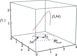
Figure 1: In a small ball $\mathcal{B}^{p}_{x_{0},\mu}$ about the point $X_{0}$, the predictors form the manifold $\mathcal{M}$. The response variable is a function of the predictors, which lie on this manifold. Here the manifold is of dimension $d=1$, and the number of predictors is $p=2$.

We make $n$ measurements of the predictors $X_{i}\in\mathbb{R}^{p}$, for $i=\{1,\ldots,n\}$, where the $X_{i}$ are independent and identically distributed. We also make $n$ noisy measurements of the function $Y_{i}=f(X_{i})+\varepsilon_{i}$, where the $\varepsilon_{i}$ are independent and identically distributed with $\mathbb{E}(\varepsilon_{i})=0$ and $\operatorname{Var}(\varepsilon_{i})=\sigma^{2}$. Let $\kappa,M>0$ be finite constants, and assume the following:

1. The kernel function $K(\cdot)$, which is used to localize our estimator by selecting points within a small region of predictor-space, is three-times differentiable and radially symmetric. These imply that $K(\cdot)$ and $K^{\prime\prime}(\cdot)$ are even functions, while $K^{\prime}(\cdot)$ is an odd function.

2. The bandwidth $h$ is the radius of predictor points about $X_{0}$ which are used by our estimator, and it has the following asymptotic rate: $h=\kappa n^{-1/(d+4)}$.

3. The kernel $K(\cdot)$ either has exponential tails or a finite support bickelli2007 . Mathematically speaking,

   $$\mathbb{E}\bigl{[}K^{\gamma}\bigl{(}(X-x)/h\bigr{)}w(X)\mathbh{1}\bigl{(}X\in(\mathcal{B}^{p}_{x,h^{1-\varepsilon}})^{c}\bigr{)}\bigr{]}=o(h^{d+4}),$$

   for $\gamma\in\{1,2\}$, $0<\varepsilon<1$ and $|w(x)|\leq M(1+|x|^{2})$.

4. The local chart $\phi(\cdot)$ which is used to define the manifold in (1) is invertible and three-times differentiable within its domain. The manifold $\mathcal{M}$ is a differentiable manifold, and the function $f(\cdot)$ is three-times differentiable: $\|\partial_{i}\partial_{j}\partial_{k}(f\circ\phi)\|_{\infty}\leq M$.

5. The probability density cannot be defined in the ambient space because the Lebesgue measure of a manifold is generally zero. We have to define the probability density with respect to a $d$-dimensional measure by inducing the density with the map $\phi(\cdot)$ bickelli2007 . We define:

   $$\mathbb{P}(X\in\mathcal{S})=\mathbb{Q}\bigl{(}Z\in\phi^{-1}(\mathcal{S})\bigr{)},$$

   where $\mathcal{S}\subseteq\mathbb{R}^{p}$. The density $\mathbb{Q}(\cdot)$ is denoted by $F(z)$, and we assume that it is three-times differentiable and strictly positive at $(z=0)\in\phi^{-1}(X_{0})$.

6. The Tikhonov-type regularization parameter $\lambda_{n}$ is nondecreasing and satisfies the following rates: $\lambda_{n}/nh^{d+2}\rightarrow\infty$ and $h\lambda_{n}/nh^{d+2}\rightarrow 0$. The lasso-type regularization parameter $\mu_{n}$ is nonincreasing and satisfies the following rates: $\mu_{n}(nh^{d+2})^{-1/2}\rightarrow 0$ and $\mu_{n}(nh^{d+2})^{(\gamma-1)/2}\rightarrow\infty$.

The choice of the local chart $\phi(\cdot)$ is not unique; we could have chosen a different local chart $\psi(\cdot)$. Fortunately, it can be shown that our results are invariant under the change of coordinates $\psi^{-1}\circ\phi$ as long as the measure $\mathbb{Q}(\cdot)$ is defined to follow suitable compatibility conditions under arbitrary, smooth coordinate changes. This is important because it tells us that our results are based on the underlying geometry of the problem.

3 Change in rank of local covariance estimates

To localize the regression problem, we use kernels, bandwidth matrices and weight matrices. We define the scaled kernel $K_{h}(U)=h^{-p}K(U/h)$, where $h$ is a bandwidth. The weight matrix centered at $X_{0}$ with bandwidth $h$ is given by

$$W_{x_{0}}=\operatorname{diag}\bigl{(}K_{h}(X_{1}-X_{0}),\ldots,K_{h}(X_{n}-X_{0})\bigr{)},$$

and the augmented bandwidth matrix is given by $H=H^{1/2}H^{1/2}$, where

$$H^{1/2}=\sqrt{nh^{d}}\left[\matrix{1&0\cr 0&h\mathbb{I}_{p\times p}}\right].$$

If we define the augmented data matrix as

$$X_{x_{0}}=\left[\matrix{1&(X_{1}-X_{0})^{\prime}\cr\vdots&\vdots\cr 1&(X_{n}-X_{0})^{\prime}}\right],$$

then the weighted Gram matrix of $X_{x_{0}}$ is

$$\hat{C}_{n}\triangleq\left[\matrix{\hat{C}_{n}^{11}&\hat{C}_{n}^{12}\cr\hat{C}_{n}^{21}&\hat{C}_{n}^{22}}\right]=h^{p}\cdot H^{-1/2}X_{x_{0}}^{\prime}W_{x_{0}}X_{x_{0}}H^{-1/2}.$$ (2)

A formal statement is given in the Appendix, but the weighted Gram matrix (2) converges in probability to the following population parameters:

$$C^{11} = F(0)\int_{\mathbb{R}^{d}}{K(d_{u}\phi\cdot u)\,du},$$

$$C^{21} = C^{12^{\prime}}=0,$$ (3)

$$C^{22} = F(0)d_{u}\phi\cdot\biggl{[}\int_{\mathbb{R}^{d}}{K\bigl{(}d_{u}\phi(0)\cdot u\bigr{)}uu^{\prime}\,du}\biggr{]}\cdot d_{u}\phi^{\prime}.$$

If we expand the $\hat{C}_{n}^{22}$ term from the weighted Gram matrix (2) into

$$\hat{C}_{n}^{22}=\frac{1}{nh^{d+2-p}}\sum_{i=1}^{n}{K_{h}(X_{i}-X_{0})(X_{i}-X_{0})(X_{i}-X_{0})^{\prime}},$$ (4)

it becomes apparent that $\hat{C}_{n}^{22}$ can be interpreted as a local covariance matrix. The localizing terms associated with the kernel add a bias, and this causes problems when doing regression. The $\hat{C}_{n}^{11}$ term does not cause problems because it is akin to the denominator of the Nadaraya–Watson estimator fangijbels1996 which does not need any regularizations.

The bias of the local covariance estimate $\hat{C}_{n}^{22}$ causes problems in doing regression, because the bias can cause the rank of $\hat{C}_{n}^{22}$ to be different than the rank of $C_{n}^{22}$. The change in rank found in the general case of the local, nonlinear manifold causes problems with MP which is discontinuous when the covariance matrix changes rank aitchison1982 . In the special case of a global, linear manifold, a similar change in rank can happen because of errors-in-variables. It is worth noting that MP works well in the case of a singular design matrix.

4 Manifold regularization

To compensate for this change in rank, we use a Tikhonov-type regularization similar to RR and EN. The distinguishing feature of our estimators is the particular form of the regularizing matrix used. Our approach is to estimate the tangent plane at $X_{0}$ of the manifold $\mathcal{M}$ and then constrain the regression coefficients to lie close to the principal components of the manifold. The idea for this type of regularization is informed by the intuition of exterior derivatives. An advantage of this regularization is that it makes it easy to apply lasso-type regularizations, and this combination of the two types of regularization is similar to EN.

To constrain the regression coefficients to lie close to the manifold, we pose the problem as a weighted least-squares problem with Tikhonov-type regularization:

$$\hat{\beta}={\arg\min}\|W(Y-X\beta)\|_{2}^{2}+\lambda\|\Pi\beta\|_{2}^{2}.$$ (5)

The matrix $\Pi$ is a projection matrix chosen to penalize $\beta$ for lying off of the manifold. Contrast this to RR and EN which choose $\Pi$ to be the identity matrix. Thus, RR and EN do not fully take the manifold structure of the problem into consideration.

Stated in another way, $\Pi$ is a projection matrix which is chosen to penalize the components of $\beta$ which are perpendicular to the manifold. The cost function we are minimizing has the term $\|\Pi\beta\|_{2}^{2}$, and this term is large if $\beta$ has components perpendicular to the manifold. Components of $\beta$ parallel to the manifold are not penalized because the projection onto these directions is zero.

Since we do not know the manifold a priori, we must learn the manifold from the sample local covariance matrix $\hat{C}_{n}^{22}$. We do this by looking at the principal components of $\hat{C}_{n}^{22}$, and so our estimators are very closely related to PCR. Suppose that we do an eigenvalue decomposition of $\hat{C}_{n}^{22}$:

$$\hat{C}_{n}^{22}=\left[\matrix{\hat{U}^{R}&\hat{U}^{N}}\right]\operatorname{diag}(\lambda^{1},\ldots,\lambda^{p})\left[\matrix{\hat{U}^{R}&\hat{U}^{N}}\right]^{\prime},$$ (6)

where $\hat{U}^{R}\in\mathbb{R}^{p\times d}$, $\hat{U}^{N}\in\mathbb{R}^{p\times(p-d)}$ and $\lambda^{1}\geq\lambda^{2}\geq\cdots\geq\lambda^{p}$. Note that the eigenvalue decomposition always exists because $\hat{C}_{n}^{22}$ is symmetric. The estimate of the manifold is given by the $d$ most relevant principal components, and the remaining principal components are perpendicular to the estimated manifold.

Because we want the projection matrix $\Pi$ to project $\beta$ onto the directions perpendicular to the estimated manifold, we define the following projection matrices

$$\hat{\Pi} \triangleq \hat{U}^{N}\hat{U}^{N^{\prime}},$$

$$\hat{P} \triangleq \operatorname{diag}(0,\hat{\Pi}).$$

The choice of $d$ is a tunable parameter that is similar to the choice in PCR. These matrices act as a regularizer because $d$ can always be chosen to ensure that $\operatorname{rank}(\hat{C}_{n}^{22}+\lambda\hat{\Pi}_{n})=p$. Furthermore, we have the following theorem regarding the full regularizing matrix $\hat{P}$:

Theorem 4.1 ([Lemma .2, part (d)])

Under the assumptions given in Section 2, the following holds with probability one:

$$\operatorname{rank}(\hat{C}_{n}+\lambda_{n}\hat{P}_{n}/nh^{d+2})=p+1.$$ (8)

Our estimators can perform better than PCR because of a subtle difference. PCR requires that the estimate lies on exactly the first $d$ most relevant principal components; however, our estimator only penalizes for deviation from the $d$ most relevant principal components. This is advantageous because in practice $d$ is not known exactly and because the principal components used are estimates of the true principal components. Thus, our regularization is more robust to errors in the estimates of the principal components. Also, our new regularization allows us to easily add additional lasso-type regularization to potentially improve the estimation. PCR cannot be easily extended to have lasso-type regularization.

We denote the function value at $X_{0}$ as $f|_{x_{0}}$. Also, we denote the exterior derivative of $f(\cdot)$ at $X_{0}$ as $d_{x}f|_{x_{0}}$. Then, the true regression coefficients are denoted by the vector

$$\beta^{\prime}=\left[\matrix{f|_{x_{0}}&d_{x}f|_{x_{0}}}\right].$$ (9)

The nonparametric exterior derivative estimator (NEDE) is given by

$$\hat{\beta}=\mathop{\arg\min}_{\tilde{\beta}}\{h^{p}\|W_{x_{0}}^{1/2}(Y-X_{x_{0}}\tilde{\beta})\|_{2}^{2}+\lambda_{n}\|\hat{P}_{n}\cdot\tilde{\beta}\|_{2}^{2}\},$$ (10)

where $\hat{P}_{n}$ is defined using (4) with $\hat{C}_{n}$. We can also define a nonparametric adaptive lasso exterior derivative estimator (NALEDE) as

$$\qquad\quad\hat{\beta}=\mathop{\arg\min}_{\tilde{\beta}}\Biggl{\{}h^{p}\|W_{x_{0}}^{1/2}(Y-X_{x_{0}}\tilde{\beta})\|_{2}^{2}+\lambda_{n}\|\hat{P}_{n}\cdot\tilde{\beta}\|_{2}^{2}+\mu_{n}\sum_{j=1}^{p}{\frac{1}{\hat{w}_{j}^{\gamma}}|\tilde{\beta}_{j}|}\Biggr{\}},$$ (11)

where $\hat{P}_{n}$ is define in (4) using $\hat{C}_{n}$, $\hat{w}$ is the solution to (10), and $\gamma>0$.

Our estimators have nice statistical properties, as the following theorem shows.

Theorem 4.2

If the assumptions in Section 2 hold, then the NEDE (10) and NALEDE (11) estimators are consistent and asymptotically normal:

$$H^{1/2}(\hat{\beta}-\beta)\stackrel{{\scriptstyle d}}{{\rightarrow}}C^{{\dagger}}\mathcal{N}(B^{\prime},\sigma^{2}V),$$

where $B$ and $V$ are, respectively, given in (25) and (26), and $C^{{\dagger}}$ denotes the Moore–Penrose psuedoinverse of $C$. Furthermore, we asymptotically have that $\hat{\beta}^{\prime}\in\mathbb{R}\times T^{*}_{P}\mathcal{M}$. The NALEDE (11) estimator has the additional feature that

$$\mathbb{P}\bigl{(}\operatorname{sign}(\hat{\beta})=\operatorname{sign}(\beta)\bigr{)}\rightarrow 1.$$

Note that the asymptotic normality is biased because of the bias typical in nonparametric regression. This bias is seen in both the NEDE (10) and NALEDE (11) estimators, but examining $B$ one sees that the bias only exists for the function estimate $\hat{f}_{x_{0}}$ and not for the exterior derivative estimate $d_{x}\hat{f}|_{x_{0}}$. This bias occurs because we are choosing $h$ to converge at the optimal rate. If we were to choose $h$ at a faster rate, then there would be no asymptotic bias, but the estimates would converge at a slower rate.

It is worth noting that the rate of convergence in Theorem 4.2 has an exponential dependence on the dimension of the manifold $d$, and our particular rates are due to the assumption of the existence of three derivatives. As is common with local regression, it is possible to improve the rate of convergence by using local polynomial regression which assumes the existence of higher-order derivatives ruppertwand1994 , bickelli2007 . However, the general form of local polynomial regression on manifolds would require the choice of a particular chart $\phi(\cdot)$ and domain $\mathcal{U}$. Local linear regression on manifolds is unique in that one does not have to pick a chart and domain.

As a last note, recall that the rate of convergence in Theorem 4.2 depends on the dimension of the manifold $d$ and does not depend on the dimension $p$ of the ambient space. We might mistakenly think that this means that the estimator converges in the “large $p$, small $n$” scenario, but without additional assumptions these results are only valid for when $p$ grows more slowly than $n$. Analogous to other “large $p$, small $n$” settings, if we assume sparsity then we can achieve faster rates of convergence, which is the subject of the next section.

5 Large $p$, small $n$

We consider extensions of our estimators to the “large $p$, small $n$” setting. The key difference in this case is the need to regularize the covariance matrix. Our NEDE (10) and NALEDE (11) estimators use the eigenvectors of the sample covariance matrix, and it is known ledoitwolf2003 , bickellevina2008 that the sample covariance matrix is poorly behaved in the “large $p$, small $n$” setting. To ensure the sample eigenvectors are consistent estimates, we must use some form of covariance regularization ledoitwolf2003 , zouetal2006 , bickellevina2008 .

We use the regularization technique used in bickellevina2008 for ease of analysis and because other regularization techniques ledoitwolf2003 , zouetal2006 do not work when the true covariance matrix is singular. The scheme in bickellevina2008 works by thresholding the covariance matrix, which leads to consistent estimates as long as the threshold is correctly chosen. We define the thresholding operator as

$$T_{t}(m)=m\mathbh{1}(|m|>t),$$

and by abuse of notation $T_{t}(M)$ is $T_{t}(\cdot)$ applied to each element of $M$.

The setup and assumptions are nearly identical to those of the fixed $p$ case described in Section 2. The primary differences are that (a) $d,p,n$ increase at different rates toward infinity, and (b) there is some amount of sparsity in the manifold and in the function. The population parameters $C_{n}$, analogous to (3), are functions of $n$ and are defined in nearly the same manner, except with $[C_{n}^{21}]_{k}=F(0)/2\int_{\mathbb{R}^{d}}{K(d_{u}\phi\cdot u)\partial_{ij}\phi^{k}u^{i}u^{j}\,du}$. Their estimates are now defined

$$\hat{C}_{n}=H^{-1}X_{x_{0}}^{\prime}W_{x_{0}}X_{x_{0}};$$

compare this to (2). Just as $C_{n}$ can be interpreted as a local covariance matrix, we now define a local cross-covariance matrix:

$$R_{n}=\left[\matrix{R_{n}^{1}\vspace*{2pt}\cr R_{n}^{2}}\right]=\left[\matrix{C_{n}^{11}\cdot f|_{x_{0}}\vspace*{2pt}\cr C_{n}^{21}\cdot f|_{x_{0}}+C_{n}^{22}\cdot d_{x}f|_{x_{0}}}\right],$$

and the estimates are given by

$$\hat{R}_{n}=H^{-1/2}X_{x_{0}}^{\prime}W_{x_{0}}Y.$$

For the sake of brevity, we summarize the other the differences from Section 2. The following things are different:

1. The manifold $\mathcal{M}_{n}$, local chart $\phi_{n}(\cdot)$, manifold dimension $d_{n}$, number of predictors $p_{n}$, and density function $F_{n}(\cdot)$ are all functions of $n$. We drop the subscript $n$ when it is clear from the context. These objects are defined in the same manner as in Section 2, and we additionally assume that the density $F(\cdot)$ is Lipschitz continuous.

2. The asymptotic rates for $d,p,n$ are given by $d=o(\log n)$,

   $$h = o\bigl{(}(c_{n}^{4}n/\log p)^{-1/(4+d)}\bigr{)},$$

   $$c_{n}\sqrt{\frac{\log p}{nh^{d}}} = o(1);$$

   where $c_{n}$ is a measure of sparsity that describes the number of nonzero entries in covariance matrices, exterior derivative, etc.

3. The kernel $K(\cdot)$ has finite support and is Lipschitz continuous, which implies that

   $$K\biggl{(}\frac{\phi(hu)-\phi(0)}{h}\biggr{)}=K(d_{u}\phi\cdot u)=0,$$

   for $u\notin\mathcal{B}^{d_{n}}_{0,\Omega}$. Contrast this to the second assumption in Section 2.

4. The local chart $\phi_{n}(\cdot)$, function $f_{n}(\cdot)$ and local (cross-)covariance matrices $C_{n},R_{n}$ satisfy the following sparsity conditions:

   $$\sum_{k=1}^{p}{\mathbh{1}(Q^{k}\neq 0)}\leq c_{n}\quad\mbox{and}\quad|Q^{k}|\leq M,$$ (12)

   for (derivatives of the local chart; the index $k$ denotes the $k$th component of the vector-valued $\phi$) $Q^{k}=\partial_{i}\phi^{k},\partial_{ij}\phi^{k},\partial_{ijm}\phi^{k},\partial_{ijmn}\phi^{k}$; for (derivatives of the function) $Q^{k}=[d_{x}f]_{k},\partial_{ik}(f\circ\phi),\partial_{ijk}(f\circ\phi)$; and for (local covariance matrices) $Q^{k}=[C_{n}]_{ik},[R_{n}]_{ik}$.

5. The smallest, nonzero singular value of the local covariance matrix is bounded. That is, there exists $\varepsilon>0$ such that

   $$\inf_{n>0}\Bigl{(}\inf_{\sigma(\cdot)>0}\sigma(C_{n})\Bigr{)}>\varepsilon.$$ (13)

   This condition ensures that the regularized inverse of the local covariance matrix is well defined in the limit; otherwise we could have a situation with ever-decreasing nonzero singular values.

6. The Tikhonov-type regularization parameter $\lambda_{n}$ and the lasso-type regularization parameter $\mu_{n}$ have the following asymptotic rates:

   $$\displaystyle\lambda_{n}=O_{p}\biggl{(}\sqrt{c_{n}}\biggl{(}\frac{nh^{d}}{\log p}\biggr{)}^{1/4}\biggr{)},$$

   $$\displaystyle\mu_{n}c_{n}^{3/2}\biggl{(}\frac{\log p}{nh^{d}}\biggr{)}^{1/4}=o(1),$$

   $$\displaystyle\mu_{n}\biggl{(}c_{n}^{3/2}\biggl{(}\frac{\log p}{nh^{d}}\biggr{)}^{1/4}\biggr{)}^{1-\gamma}\rightarrow\infty.$$

7. The threshold which regularizes the local sample covariance matrix is given by

   $$t_{n}=K\sqrt{\frac{\log p}{n}},$$ (14)

   where $\frac{\log p}{n}=o(1)$. This regularization will make the regression estimator consistent in the “large $p$, small $n$” case.

5.1 Manifold regularization

The idea is to regularize the local sample covariance matrix by thresholding. If the true, local covariance matrix is sparse, this regularization will give consistent estimates. This is formalized by the following theorem.

Theorem 5.1

If the assumptions given in Section 5 are satisfied, then

$$\|T_{t}(\hat{C}_{n})-C_{n}\| = O_{p}\bigl{(}c_{n}\sqrt{\log p/nh^{d}}\bigr{)},$$

$$\|T_{t}(\hat{R}_{n})-R_{n}\| = O_{p}\bigl{(}c_{n}\sqrt{\log p/nh^{d}}\bigr{)}.$$

Once we have consistent estimates of the true, local covariance matrix, we can simply apply our manifold regularization scheme described in Section 4. The nonparametric exterior derivative estimator for the “large $p$, small $n$” case (NEDEP) is given by

$$\hat{\beta}_{n}=\mathop{\arg\min}_{\tilde{\beta}}\bigl{\|}\bigl{(}T_{t}(\hat{C}_{n})+\lambda_{n}\hat{P}_{n}\bigr{)}\tilde{\beta}-T_{t}(\hat{R}_{n})\bigr{\|}_{2}^{2},$$ (15)

where $\hat{P}_{n}$ is as defined in (4) except using $T_{t}(\hat{C}_{n}^{22})$. The nonparametric adaptive lasso exterior derivative estimator for the “large $p$, small $n$” case (NALEDEP) is given by

$$\hat{\beta} = \mathop{\arg\min}_{\tilde{\beta}}\mathop{\arg\min}_{\tilde{\beta}}\bigl{\|}\bigl{(}T_{t}(\hat{C}_{n})+\lambda_{n}\hat{P}_{n}\bigr{)}\tilde{\beta}-T_{t}(\hat{R}_{n})\bigr{\|}_{2}^{2}$$

$${}+\mu_{n}\sum_{j=1}^{p}{\frac{1}{\hat{w}_{j}^{\gamma}}|\tilde{\beta}_{j}|},$$

where $\hat{P}_{n}$ is as defined in (4) except using $T_{t}(\hat{C}_{n}^{22})$ and $\hat{w}$ is the solution to (15). These estimators have nice statistical properties.

Theorem 5.2

If the assumptions given in Section 5 are satisfied, then the NALEDE (15) and NALEDEP (5.1) estimators are consistent:

$$\|\hat{\beta}-\beta\|_{2}=O_{p}\biggl{(}c_{n}^{3/2}\biggl{(}\frac{\log p}{nh^{d}}\biggr{)}^{1/4}\biggr{)}.$$

The NALEDEP (5.1) estimator is also sign consistent:

$$\mathbb{P}\bigl{(}\operatorname{sign}(\hat{\beta})=\operatorname{sign}(\beta)\bigr{)}\rightarrow 1.$$

We do not give a proof of this theorem, because it uses essentially the same argument as Theorem 5.3. One minor difference is that the proof uses our Theorem 5.1 instead of Theorem 1 from bickellevina2008 .

5.2 Linear case

Our estimators admit simple extensions in the special case where predictors lie on a global, linear manifold and the response variable is a linear function of the predictors. We specifically consider the errors-in-variables situation with manifold structure in order to present our formal results, because: in principle, our estimators provide no improvements in the linear manifold case over existing methods when there are no errors-in-variables. In practice, our estimators sometimes provide an improvement in this case. Furthermore, our estimators provide another solution to the identifiability problem fu2008 ; the exterior derivative is the unique set of regression coefficients because the predictors are only sampled in directions parallel to the manifold, and there is no derivative information about the response variable in directions perpendicular to the manifold.

Suppose there are $n$ data points and $p$ predictors, and the dimension of the global, linear manifold is $d$. We assume that $d,n,p$ increase to infinity, and leaving $d$ fixed is a special case of our results. We consider a linear model $\eta=\Xi\overline{\beta}$, where $\eta\in\mathbb{R}^{n\times 1}$ is a vector of function values, $\Xi\in\mathbb{R}^{n\times p}$ is a matrix of predictors, and $\overline{\beta}\in\mathbb{R}^{p}$ is a vector.

The $\Xi$ are distributed according to the covariance matrix $\Sigma_{\xi}$, which is also a singular design matrix in this case. The exterior derivative of this linear function is given by $\beta=P_{\Sigma_{\xi}}\overline{\beta}$, where $P_{\Sigma_{\xi}}$ is the projection matrix that projects onto the range space of $\Sigma_{\xi}$. We make noisy measurements of $\eta$ and $\Xi$:

$$X = \Xi+\nu,$$

$$Y = \eta+\varepsilon.$$

The noise $\nu$ and $\varepsilon$ are independent of each other, and each component of $\nu$ is independent and identically distributed with mean $0$ and variance $\sigma_{\nu}^{2}$. Similarly, each component of $\varepsilon$ is independent and identically distributed with mean $0$ and variance $\sigma^{2}$. In this setup, the variance $\sigma_{\nu}^{2}$ is identifiable kritchmannadler2008 , johnstonelu2009 , and an alternative that works well in practice for low noise situations is to set this quantity to zero.

Our setup with errors-in-variables is different from the setup of existing tools candestao2007 , meinshausenyu2006 , but it is important because in practice, many of the near-collinearities might be true collinearities that have been perturbed by noise. Several formulations explicitly introduce noise into the model kritchmannadler2008 , nadler2008 , carrolmacaruppert1999 , fantruong1993 , johnstonelu2009 . We choose the setting of kritchmannadler2008 , johnstonelu2009 , because the noise in the predictors is identifiable in this situation.

The exterior derivative estimator for the “large $p$, small $n$” case (EDEP) is given by

$$\hat{\beta}=\mathop{\arg\min}_{\tilde{\beta}}\bigl{\|}\bigl{(}T_{t}(X^{\prime}X/n)-\sigma_{\nu}^{2}\mathbb{I}+\lambda_{n}\hat{P}_{n}\bigr{)}\tilde{\beta}-T_{t}(X^{\prime}Y/n)\bigr{\|}_{2}^{2},$$ (17)

where $\hat{P}_{n}$ is as defined in (4) except applied to $\hat{C}_{n}^{22}=T_{t}(X^{\prime}X/n)-\sigma_{\nu}^{2}\mathbb{I}$. This is essentially the NEDEP estimator, except the weighting matrix is taken to be the identity matrix and there are additional terms to deal with errors-in-variables. We can also define an adaptive lasso version of our estimator. The adaptive lasso exterior derivative estimator for the “large $p$, small $n$” case (ALEDEP) is given by

$$\hat{\beta} = \mathop{\arg\min}_{\tilde{\beta}}\bigl{\|}\bigl{(}T_{t}(X^{\prime}X/n)-\sigma_{\nu}^{2}\mathbb{I}+\lambda_{n}\hat{P}_{n}\bigr{)}\tilde{\beta}-T_{t}(X^{\prime}Y/n)\bigr{\|}_{2}^{2}$$

$${}+\mu_{n}\sum_{j=1}^{p}{\frac{1}{\hat{w}_{j}^{\gamma}}|\tilde{\beta}_{j}|},$$

where $\hat{P}_{n}$ is as defined in (4) except applied to $\hat{C}_{n}^{22}=T_{t}(X^{\prime}X)-\sigma_{\nu}^{2}\mathbb{I}$ and $\hat{w}$ is the solution to (17). We can analogously define the EDE and ALEDE estimators which are the EDEP and ALEDEP estimators without any thresholding. In practice, setting the value of the $\sigma_{\nu}^{2}$ term equal to zero seems to work well with actual data sets.

The technical conditions we make are essentially the same as those for the case of the local, nonlinear manifold. The primary difference is that we ask that the conditions in Section 5 hold globally, instead of locally. This also means that we do not use any kernels to localize the estimators, and the $W$ matrix in the estimators is simply the identity matrix. If the theoretical rates for the regularization and threshold parameters are compatibility redefined, then we can show that these estimators have nice statistical properties.

Theorem 5.3

If the assumptions in Sections 5 and 5.2 hold, then the EDEP (17) and ALEDEP (5.2) estimators are consistent. They asymptotically converge at the following rate:

$$\|\hat{\beta}-\beta\|_{2}=O_{p}\biggl{(}c_{n}^{3/2}\biggl{(}\frac{\log p}{n}\biggr{)}^{1/4}\biggr{)}.$$

The ALEDE (5.2) estimator is also sign consistent:

$$\mathbb{P}\bigl{(}\operatorname{sign}(\hat{\beta})=\operatorname{sign}(\beta)\bigr{)}\rightarrow 1.$$ (19)

Our theoretical rate of convergence is slower than that of other techniques candestao2007 , meinshausenyu2006 because we have applied our technique for local estimation to global estimation, and we have not fully exploited the setup of the global case. However, we do get faster rates of convergence in our global case versus our local case. Furthermore, our model has errors-in-variables, while the model used in other techniques candestao2007 , meinshausenyu2006 assumes that the predictors are measured with no noise. Applying the various techniques to both real and simulated data shows that our estimators perform comparably to or better than existing techniques. It is not clear if the rates of convergence for the existing techniques candestao2007 , meinshausenyu2006 would be slower if there were errors-in-variables, and this would require additional analysis.

6 Estimation with data

Applying our estimators in practice requires careful usage. The NEDE estimator requires the choice of two tuning parameters, while the NALEDE and NEDEP estimators require choosing three; the NALEDEP estimator requires choosing four. The extra tuning parameters—in comparison to existing techniques like MP or RR—make our method prone to over-fitting. This makes it crucial to select the parameters using methods, such as cross-validation or bootstrapping, that protect against overfitting. It is also important to select from a small number of different parameter-values to protect against overfitting caused by issues related to multiple-hypothesis testing ng1997 , juha2003 , rao2008 .

Bootstrapping is one good choice for parameter selection with our estimators bickelfreedman1981 , shao1993 , shao1994 , shao1996 , bickellevina2008 . Additionally, we suggest selecting parameters in a sequential manner; this is to reduce overfitting caused by testing too many models ng1997 , juha2003 , rao2008 . Another benefit of this approach is that it simplifies the parameter selection into a set of one-dimensional parameter searches—greatly reducing the computational complexity of our estimators. For instance, we first select the Tikhonov-regularization parameter $\lambda$ for RR. Using the same $\lambda$ value, we pick the dimension $d$ for the NEDE estimator. The prior values of $\lambda$ and $d$ are used to pick the lasso-regularization parameter $\mu$ for the NALEDE estimator.

MATLAB implementations of both related estimators and our estimators can be found online. The lasso-type regressions were computed using the coordinate descent algorithm FHHT2007 , wulange2008 , and we used the “improved kernel PLS by Dayal” code given in anderson2009 to do the PLS regression. The increased computational burden of our estimators, as compared to existing estimators, is reasonable because of: improved estimation in some cases, easy parallelization, and computational times of a few seconds to several minutes on a general desktop for moderate values of $p$.

7 Numerical examples

We provide three numerical examples: the first two examples use simulated data, and the third example uses real data. In the examples with simulated data, we study the estimation accuracy of various estimators as the amount of noise and number of data points vary. The third example uses the Isomap face data used in tenenbaumetal2000 . In the example, we do a regression to estimate the pose of a face based on an image.

For examples involving linear manifolds and functions, we compare our estimators with popular methods. The exterior derivative is locally defined, but in the linear case it is identical at every point—allowing us to do the regression globally. This is in contrast to the example with a nonlinear manifold and function where we pick a point to do the regression at. Though MP, PLS, PCR, RR and EN are typically thought of as global methods, we can use these estimators to do local, nonparametric estimation by posing the problem as a weighted, linear regression which can then be solved using either our or existing estimators. As a note, the MP and OLS estimators are equivalent in the examples we consider.

Some of the examples involve errors-in-variables, and this suggests that we should use an estimator that explicitly takes this structure into account. We compared these methods with Total Least Squares (TLS) vanhuffelvandewalle1991 which does exactly this. TLS performed poorly with both the simulated data and experimental data, and this is expected because standard TLS is known to perform poorly in the presence of collinearities vanhuffelvandewalle1991 . TLS performed comparably to or worse than OLS/MP, and so the results are not included.

Based on the numerical examples, it seems that the improvement in estimation error of our estimators is mainly due to the Tikhonov-type regularization, with lasso-type regularization providing additional benefit. Thresholding the covariance matrices did not make significant improvements, partly because bootstrap has difficulty with picking the thresholding parameter. Improvements may be possible by refining the parameter selection method or by changes to the estimator. We also observed the well-known tendency of lasso to overestimate the number of nonzero coefficients mb2009 ; using stability selection mb2009 to select the lasso parameter would likely lead to better results.

7.1 Simulated data

We simulate data for two different models and use this to compare different estimators. One model is linear, and we do global estimation in this case. The other model is nonlinear, and hence we do local estimation in this case. In both models, there are $p$ predictors and the dimension of the manifold is $d=\operatorname{round}(\frac{3}{4}p)$. The predictors $\xi$ and response $\eta$ are measured with noise:

$$x = \xi+\mathcal{N}(0,\sigma_{\nu}^{2}),$$

$$y = \eta+\mathcal{N}(0,\sigma^{2}).$$

And for notational convenience, let $q=\operatorname{round}(\frac{1}{2}p)$. Define the matrix

$$F_{ij}=\cases{0.3^{|i-j|},&\quad if $1\leq i,j\leq d$,\cr 0.3,&\quad if $d+1\leq i\leq p\wedge j=q+i-d$,\cr 0.3,&\quad if $d+1\leq i\leq p\wedge j=q+i+1-d$,\cr 0,&\quad o.w.}$$

The two models are given by:

1. Linear model: the predictors are distributed $\xi=\mathcal{N}(0,FF^{\prime})$, and the function is

   $$\eta=f(\xi)=1+\mathop{\sum_{i=1}}_{i\ \mathrm{is}\ \mathrm{odd}}^{q}\xi_{i}.$$ (20)

   If $w=[1\enskip 0\enskip 1\enskip\cdots]$ is a vector with ones in the odd index-positions and zeros elsewhere, then the exterior derivative of this linear function at every point on the manifold is given by the projection of $w$ onto the range space of the matrix $F$.

2. Nonlinear model: the predictors are distributed $\xi=\sin(\mathcal{N}(0,FF^{\prime}))$, and the function is

   $$\eta=f(\xi)=1+\mathop{\sum_{i=1}}_{i\ \mathrm{is}\ \mathrm{odd}}^{q}\sin(\xi_{i}).$$ (21)

   We are interested in local regression about the point $x_{0}=[0\enskip\cdots\enskip 0]$. If $w=[1\enskip 0\enskip 1\enskip\cdots]$ is a vector with ones in the odd index-positions and zeros elsewhere, then the exterior derivative of this nonlinear function at the origin is given by the projection of $w$ onto the range space of the matrix $F$.

Table 1 shows the average square-loss estimation error $\|\hat{\beta}-\beta\|_{2}^{2}$ for different estimators using data generated by the linear model and nonlinear model given above, over

Table 1: Averages and standard deviations over 100 replications of square-loss estimation error for different estimators using data generated by the linear model and nonlinear model given in Section 7.1, over different noise variances and number of data points $n$

	$\bolds{n=10}$		$\bolds{n=100}$		$\bolds{n=1000}$
	Linear model: $\sigma_{\nu}^{2}=0.01,\sigma^{2}=1.00$
OLS/MP	3.741	(2.476)	6.744	(3.602)	0.588	(0.368)
RR	2.523	(1.020)	0.369	(0.193)	0.167	(0.086)
EN	2.562	(1.054)	0.117	(0.197)	0.017	(0.008)
PLS	2.428	(0.536)	0.501	(0.207)	0.031	(0.013)
PCR	3.391	(0.793)	1.629	(0.144)	1.583	(0.047)
EDE	2.528	(1.030)	0.367	(0.185)	0.166	(0.086)
ALEDE	2.564	(1.061)	0.111	(0.177)	0.015	(0.006)
EDEP	2.527	(1.025)	0.370	(0.184)	0.167	(0.085)
ALEDEP	2.563	(1.057)	0.111	(0.177)	0.015	(0.006)
	Linear model: $\sigma_{\nu}^{2}=0.10,\sigma^{2}=1.00$
OLS/MP	3.629	(1.488)	1.259	(0.598)	0.173	(0.050)
RR	2.717	(0.847)	0.892	(0.351)	0.260	(0.042)
EN	2.783	(0.895)	0.661	(0.523)	0.064	(0.013)
PLS	2.588	(0.566)	0.740	(0.252)	0.138	(0.037)
PCR	3.425	(0.747)	1.645	(0.144)	1.569	(0.047)
EDE	2.716	(0.846)	0.840	(0.305)	0.255	(0.042)
ALEDE	2.782	(0.893)	0.590	(0.459)	0.050	(0.013)
EDEP	2.720	(0.849)	0.841	(0.305)	0.255	(0.042)
ALEDEP	2.784	(0.895)	0.590	(0.459)	0.050	(0.013)

different noise variances and number of data points $n$. We conducted 100 replications of generating data and doing a regression, and this helped to provide standard deviations of square-loss estimation error to show the variability of the estimators. Table 2 shows computation times in seconds for the different estimators; it shows that our estimators require more computation, but the computation time is still reasonable. The computation time does not depend on the noise level, and so we have averaged the computation times over the $100+100$ replications for $\sigma_{\nu}^{2}=0.01,0.10$.

Table 1: (Continued)

	$\bolds{n=20}$		$\bolds{n=100}$		$\bolds{n=1000}$
	Nonlinear model: $\sigma_{\nu}^{2}=0.01,\sigma^{2}=1.00$
OLS/MP	657.700	(1842)000.	3.797	(2.172)	0.367	(0.223)
RR	2.188	(0.715)	1.160	(0.265)	0.300	(0.132)
EN	2.140	(0.768)	1.083	(0.341)	0.162	(0.081)
PLS	2.102	(0.757)	0.995	(0.256)	0.172	(0.120)
PCR	2.731	(0.439)	1.679	(0.244)	0.123	(0.043)
NEDE	2.184	(0.716)	1.104	(0.269)	0.288	(0.118)
NALEDE	2.136	(0.769)	1.009	(0.357)	0.144	(0.067)
NEDEP	2.184	(0.716)	1.103	(0.269)	0.288	(0.118)
NALEDEP	2.136	(0.769)	1.008	(0.357)	0.144	(0.067)
	Nonlinear model: $\sigma_{\nu}^{2}=0.1,\sigma^{2}=1.00$
OLS/MP	147.500	(338.3)00	1.843	(0.975)	0.473	(0.110)
RR	2.693	(1.793)	1.260	(0.369)	0.672	(0.139)
EN	2.698	(1.927)	1.168	(0.455)	0.472	(0.197)
PLS	2.385	(0.629)	1.210	(0.318)	0.768	(0.133)
PCR	2.767	(0.450)	1.766	(0.293)	0.554	(0.348)
NEDE	2.694	(1.793)	1.233	(0.352)	0.641	(0.119)
NALEDE	2.702	(1.925)	1.126	(0.445)	0.407	(0.130)
NEDEP	2.693	(1.794)	1.231	(0.352)	0.641	(0.119)
NALEDEP	2.702	(1.926)	1.124	(0.445)	0.407	(0.130)

Table 2: Averages and standard deviations over 200 replications of computation times in seconds for the different estimators using data generated by the linear model and nonlinear model given in Section 7.1

	$\bolds{n=10}$		$\bolds{n=100}$		$\bolds{n=1000}$
	Linear model
OLS/MP	0.001	(0.000)	0.001	(0.000)	0.001	(0.000)
RR	0.055	(0.005)	0.063	(0.005)	0.110	(0.004)
EN	1.739	(1.325)	0.292	(0.032)	0.387	(0.042)
PLS	1.631	(0.029)	1.716	(0.077)	1.925	(0.051)
PCR	0.185	(0.006)	0.192	(0.010)	0.253	(0.007)
EDE	0.239	(0.007)	0.255	(0.016)	0.367	(0.021)
ALEDE	2.071	(1.363)	0.715	(0.043)	0.912	(0.059)
EDEP	0.411	(0.011)	0.523	(0.019)	0.731	(0.052)
ALEDEP	2.248	(1.366)	0.990	(0.042)	1.283	(0.083)
	$\bolds{n=20}$		$\bolds{n=100}$		$\bolds{n=1000}$
	Nonlinear model
OLS/MP	0.001	(0.000)	0.001	(0.000)	0.001	(0.000)
RR	0.359	(0.039)	0.470	(0.028)	0.938	(0.040)
EN	0.916	(0.433)	1.005	(0.058)	1.917	(0.269)
PLS	1.980	(0.130)	2.114	(0.072)	2.879	(0.162)
PCR	1.014	(0.062)	1.118	(0.038)	1.911	(0.166)
NEDE	0.840	(0.078)	1.066	(0.058)	2.031	(0.092)
NALEDE	2.175	(0.594)	1.843	(0.090)	3.381	(0.401)
NEDEP	1.403	(0.120)	1.726	(0.087)	2.277	(0.175)
NALEDEP	2.671	(0.647)	2.513	(0.122)	4.631	(0.397)

One curious phenomenon observed is that the estimation error goes down in some cases as the error variance of the predictors $\sigma_{\nu}^{2}$ increases. To understand why, consider the sample covariance matrix in the linear case $\hat{S}=X^{\prime}X/n$ with population parameter $S=FF^{\prime}+\sigma_{\nu}^{2}\mathbb{I}$. Heuristically, the OLS estimate will tend to $(FF^{\prime}+\sigma_{\nu}^{2}\mathbb{I})^{-1}X^{\prime}Y/n$, and the error in the predictors actually acts as the Tikhonov-type regularization found in RR, with lower levels of noise leading to less regularization.

The results indicate that our estimators are not significantly more variable than existing ones, and our estimators perform competitively against existing estimators. Though our estimators are closely related to PCR, RR and EN, our estimators performed comparably to or better than these estimators. PLS also did quite well, and our estimators did better than PLS in some cases. Increasing the noise in the predictors did not seem to significantly affect the qualitative performance of the estimators, except for OLS as explained above.

In Section 5.2, we discussed how the converge rate of our linear estimators is of order $n^{-1/4}$ which is in contrast to the typical convergence rate of $n^{-1/2}$ for lasso-type regression meinshausenyu2006 . We believe that this theoretical discrepancy is because our model has errors-in-variables while the standard model used in lasso-type regression does not meinshausenyu2006 . These theoretical differences do not seem significant in practice. As seen in Table 1, our estimators can be competitive with existing lasso-type regression.

7.2 Isomap face data

The Isomap face data from tenenbaumetal2000 consists of images of an artificial face. The images are labeled with and vary depending upon three variables: illumination-, horizontal- and vertical-orientation; sample images taken from this data set can be seen in Figure 2. Three-dimensional images of the face would form a three-dimensional manifold (each dimension corresponding to a variable), but this data set consists of two-dimensional projections of the face. Intuitively, a limited number of additional variables are needed for different views of the face (e.g., front, profile, etc.). This intuition is confirmed by dimensionality estimators which estimate that the two-dimensional images form a low-dimensional manifold levinabickel2005 .

To compare the different estimators, we did 100 replications of the following experiment: we randomly split the data ($n=698$ data points) into a training set $n_{t}=688$ and validation set $n_{v}=10$, and then we used the training set to estimate the horizontal pose angle of images in the validation set. Since we are doing local linear estimation, the estimate for each image requires its own regression. The number of predictors $p$ is large in this case because each data point $X_{i}$ is a two-dimensional image. Estimation when $p$ is large is computationally slow, and so we chose a small validation set size to ensure that the experiments completed in a reasonable amount of time. Replicating this experiment 100 times helps to prevent spurious results due to having a small validation set.

To speed up the computations further, we scaled the images from $64\times 64$ pixels to $7\times 7$ pixels in size. This is a justifiable approach because the images form a low-dimensional manifold, and so this resizing of the images does not lead to a loss in predictor information wright2009 . This leads to significantly faster computations, because this process reduces the number of predictors from $p=4096$ to $p=49$. In practice, our choice of $p=49$ gives predictions that deviate from the true horizontal pose angle of images (which uniformly ranges between $-$75 to 75 degrees) in the validation set by a root-mean-squared error of three degrees or less.

Figure 2: Sample images from the Isomap face data tenenbaumetal2000 . The images are labeled with and vary depending upon three variables: illumination-, horizontal- and vertical-orientation.

Table 3: Averages and standard deviations over 100 replications of validation set prediction error for different estimators using the Isomap face data tenenbaumetal2000 . The average computation time and its standard deviation is given in seconds, and it gives the time to estimate the horizontal pose angle of a single image

	Prediction error		Computation time
OLS/MP	$5.276$	$(11.06)$	$0.002$	(0.001)
RR	$5.286$	$(6.156)$	$2.052$	(0.166)
EN	$5.168$	$(6.112)$	$17.79$	(5.235)
PLS	$10.12$	$(14.84)$	$16.22$	(0.841)
PCR	$5.813$	$(7.617)$	$8.877$	(0.609)
NEDE	$4.523$	$(4.926)$	$4.740$	(0.347)
NALEDE	$4.409$	$(4.889)$	$22.94$	(5.349)
NEDEP	$4.527$	$(4.925)$	$7.777$	(0.511)
NALEDEP	$4.406$	$(4.900)$	$25.77$	(5.221)

Table 3 gives the prediction error of the models generated by different estimators on the validation set. The specific quantity provided is

$${\sum_{X_{i}\in\mathcal{V}}}\|\hat{\beta}^{0}(X_{i})-Y_{i}\|_{2}^{2}/n_{v},$$ (22)

where $\mathcal{V}$ is the set of predictors in the validation set, $\hat{\beta}^{0}(X_{i})$ is the first component of the estimated regression coefficients computed about the point $X_{0}=X_{i}$, and $Y_{i}$ is the corresponding horizontal pose angle of the image $X_{i}$. The regression is computed using only data taken from the training set. The results from this real data set shows that our estimators can provide improvements over existing tools, because our estimators have the lowest prediction errors. Table 3 also provides the computation times for estimating the horizontal pose, and it again shows that our estimators require more computation but not by an excessively larger amount.

8 Conclusion

By interpreting collinearity as predictors on a lower-dimensional manifold, we have developed a new regularization, which has connections to PCR and RR, for linear regression and local linear regression. This viewpoint also allows us interpret the regression coefficients as estimates of the exterior derivative. We proved the consistency of our estimators in both the classical case and the “large $p$, small $n$” case and this is useful from a theoretical standpoint.

We provided numerical examples using simulated and real data which show that our estimators can provide improvements over existing estimators in estimation and prediction error. Though our estimators provide modest improvements over existing ones, these improvements are consistent over the different examples. Specifically, the Tikhonov-type and lasso-type regularizations provided improvements, and the thresholding regularization did not provide major improvements. This is not to say that thresholding is not a good regularization, because as we showed: from a theoretical standpoint, thresholding does provide consistency in the “large $p$, small $n$” situation. This leaves open the possibility of future work on how to best select this thresholding parameter value.

There is additional future work possible on extending our set of estimators. There is some benefit provided by shrinkage from the Tikhonov-type regularization which is independent of the manifold structure. Exploring more fully the relationship between manifold structure and shrinkage will likely lead to improved estimators.

Appendix

In this section, we provide the proofs of our theorems. We also give a few lemmas, which are needed for the proofs, that were not stated in the main text.

Lemma .1

If the assumptions in Section 2 hold, then:

• $\|\mathbb{E}(\hat{C}_{n}^{22})-C^{22}\|_{2}^{2}=O(h^{4})$;

• $\|\mathbb{E}[(\hat{C}_{n}^{22}-C^{22})(\hat{C}_{n}^{22}-C^{22})^{\prime}]\|_{2}^{2}=O(1/nh^{d})$;

• $\hat{C}_{n}\stackrel{{\scriptstyle p}}{{\rightarrow}}C$.

This proof follows the techniques of ruppertwand1994 , bickelli2007 . We first prove part (c). Note that

$$\hat{C}_{n}^{11}=\frac{1}{nh^{d-p}}\sum_{i=1}^{n}{K_{h}(x_{i}-x_{0})},$$

and consider its expectation

$$\mathbb{E}(\hat{C}_{n}^{11}) = \mathbb{E}\biggl{(}\frac{1}{h^{d-p}}K_{h}(x_{i}-x_{0})\mathbh{1}\bigl{(}X\in(\mathcal{B}^{p}_{x,h^{1-\varepsilon}})\bigr{)}\biggr{)}$$

$${}+\mathbb{E}\biggl{(}\frac{h^{p}}{h^{d}}K_{h}(x_{i}-x_{0})\mathbh{1}\bigl{(}X\in(\mathcal{B}^{p}_{x,h^{1-\varepsilon}})^{c}\bigr{)}\biggr{)}$$

$$= \int_{B^{d}_{0,h^{1-\varepsilon}}}{\frac{1}{h^{d}}K\biggl{(}\frac{\phi(z)-\phi(0)}{h}\biggr{)}F(z)\,dz}+o(h^{2+p})$$

$$= \int_{\mathbb{R}^{n}}{K(d_{u}\phi\cdot u)F(0)\,du}+O(h^{2}),$$

where we have used the assumption that $K(\cdot)$ is an even function, $K^{\prime}(\cdot)$ is an odd function, and $K^{\prime\prime}(\cdot)$ is an even function.

A similar calculation shows that for

$$\hat{C}_{n}^{21}=\frac{1}{nh^{d+1-p}}\sum_{i=1}^{n}{K_{h}(x_{i}-x_{0})(x_{i}-x_{0})},$$

we have that the expectation is

$$\mathbb{E}(\hat{C}_{n}^{21})=O(h)=o(1).$$

And, a similar calculation shows that for

$$\hat{C}_{n}^{22}=\frac{1}{nh^{d+2-p}}\sum_{i=1}^{n}{K_{h}(x_{i}-x_{0})(x_{i}-x_{0})(x_{i}-x_{0})^{\prime}},$$

we have that the expectation is

$$\mathbb{E}(\hat{C}_{n}^{22})=F(0)\,d_{u}\phi\cdot\biggl{[}\int_{\mathbb{R}^{d}}{K\bigl{(}d_{u}\phi(0)\cdot u\bigr{)}uu^{\prime}\,du}\biggr{]}\cdot d_{u}\phi^{\prime}+O(h^{2}).$$

The result in part (c) follows from the weak law of large numbers. The last calculation also proves part (a).

Next, we prove part (b). For notational simplicity, let

$$T_{i}=K_{h}(x_{i}-x_{0})(x_{i}-x_{0})(x_{i}-x_{0})^{\prime}.$$

The variance is

$$\operatorname{Var}(\hat{C}_{n}^{22}) = \frac{1}{n^{2}h^{4+2d-2p}}\operatorname{Tr}\bigl{(}n\bigl{(}\mathbb{E}(T_{i}T_{i}^{\prime})-\mathbb{E}(T_{i})\mathbb{E}(T_{i})^{\prime}\bigr{)}$$

$$\hskip 70.1pt{}+n(n-1)\bigl{(}\mathbb{E}(T_{i}T_{j}^{\prime})-\mathbb{E}(T_{i})\mathbb{E}(T_{j})^{\prime}\bigr{)}\bigr{)}.$$

Since $T_{i}$ and $T_{j}$ are independent, it follows that $\mathbb{E}(T_{i}T_{j}^{\prime})-\mathbb{E}(T_{i})\mathbb{E}(T_{j})^{\prime}=0$. Next, note that

$$\mathbb{E}(T_{i}T_{i}^{\prime}) = h^{-2p}\biggl{(}\int_{B_{0,h^{1-\varepsilon}}^{d}}\biggl{(}K\biggl{(}\frac{\phi(z)-\phi(0)}{h}\biggr{)}\biggr{)}^{2}[\phi(z)-\phi(0)][\phi(z)-\phi(0)]^{\prime}$$

$$\hskip 64.2pt{}\times[\phi(z)-\phi(0)][\phi(z)-\phi(0)]^{\prime}F(z)\,dz+o(h^{d+2})\biggr{)}$$

$$= h^{d+4-2p}\biggl{(}F(0)\int_{\mathbb{R}^{d}}\bigl{(}K(d_{u}\phi\cdot u)\bigr{)}^{2}\,d_{u}\phi\cdot uu^{\prime}\cdot d_{u}\phi^{\prime}\cdot d_{u}\phi$$

$$\,\hskip 123.5pt{}\times uu^{\prime}\cdot d_{u}\phi^{\prime}\cdot du+O(h^{2})\biggr{)}.$$

Thus, the variance is given by

$$\operatorname{Var}(\hat{C}_{n}^{22}) = \frac{1}{nh^{d}}\operatorname{Tr}\biggl{(}F(0)\int_{\mathbb{R}^{d}}\bigl{(}K(d_{u}\phi\cdot u)\bigr{)}^{2}\,d_{u}\phi\cdot uu^{\prime}\cdot d_{u}\phi^{\prime}\cdot d_{u}\phi$$

$$\,\hskip 119.0pt{}\times uu^{\prime}\cdot d_{u}\phi^{\prime}\cdot du+o_{p}(1)\biggr{)}.$$

Lemma .2

If the assumptions in Section 2 hold, then the matrices $\hat{C}_{n}$, $C^{22}$, $\Pi$, $\hat{\Pi}_{n}$, $\hat{P}_{n}$, and $P$ have the following properties:

1. $\operatorname{rank}(C^{22})=d$ and $\mathcal{R}(C^{22})=T_{p}\mathcal{M}$;

2. $\mathcal{R}(\Pi)=\mathcal{N}(C^{22})$, $\mathcal{N}(\Pi)=\mathcal{R}(C^{22})$ and $\mathcal{N}(\Pi)\cap\mathcal{N}(C^{22})=\{0\}$;

3. $\|\hat{P}_{n}-P\|_{2}^{2}=\|\hat{\Pi}_{n}-\Pi\|_{2}^{2}=O_{p}(1/nh^{d})$;

4. $\mathbb{P}(\operatorname{rank}(\hat{C}_{n}+\lambda_{n}\hat{P}_{n}/nh^{d+2})=p+1)\rightarrow 1$.

To show property (a), we first show that for $M\in\mathbb{R}^{d\times d}$, where

$$M=\int_{\mathbb{R}^{d}}{K\bigl{(}d_{u}\phi(0)\cdot u\bigr{)}uu^{\prime}\,du},$$

we have that $\operatorname{rank}(M)=d$. To prove this, choose any $v\in\mathbb{R}^{d}\setminus\{0\}$ and then consider the quantity

$$v^{\prime}Mv=\int_{\mathbb{R}^{d}}{K\bigl{(}d_{u}\phi(0)\cdot u\bigr{)}v^{\prime}uu^{\prime}v\,du}.$$

By construction, $v^{\prime}uu^{\prime}v>0$ almost everywhere. Additionally, since $\phi$ is three times differentiable, we have that $K(d_{u}\phi(0)\cdot u)>0$ on a set of nonzero measure and $K(d_{u}\phi(0)\cdot u)\geq 0$ elsewhere. Thus, $v^{\prime}Mv>0$ for all $v\in\mathbb{R}^{d}\setminus\{0\}$. It follows that $M$ is symmetric and positive definite with $\operatorname{rank}(M)=d$. Since $\mathcal{M}$ is a $d$-dimensional manifold, we have that $\operatorname{rank}(d_{u}\phi)=d$ by Corollary 8.4 of lee2003 . The Sylvester Inequality sastry1999 implies that

$$\operatorname{rank}(C_{22})=\operatorname{rank}(d_{u}\phi Md_{u}\phi^{\prime})=d,$$

and this implies that

$$\mathcal{R}(C_{22})=\mathcal{R}(d_{u}\phi Md_{u}\phi^{\prime})=\mathcal{R}(d_{u}\phi).$$

However, $\mathcal{R}(d_{u}\phi)=T_{p}\mathcal{M}$, where we take $p=x_{0}$. This proves the result.

We next consider property (b). We have that

$$\sigma_{1},\ldots,\sigma_{d}\neq 0\quad\mbox{and}\quad\sigma_{d+1}=\cdots=\sigma_{p}=0,$$

because $\operatorname{rank}(C_{22})=d$ by property (a). Thus, the null-space of $C_{22}$ is given by the column-span of $U_{N}$; however, the construction of $P$ implies that the column-span of $U_{N}$ is the range-space of $P$. Ergo, $\mathcal{R}(P)=\mathcal{N}(C_{22})$. Note that the column-span of $U_{R}$ belongs to the null-space of $P$, because each column in $U_{R}$ is orthogonal—by property of the SVD—to each column in $U_{N}$. Thus, we have the dual result that $\mathcal{N}(P)=\mathcal{R}(C_{22})$. The orthogonality of $U_{R}$ and $U_{N}$ due to the SVD implies that $\mathcal{N}(P)\cap\mathcal{N}(C_{22})=\{0\}$.

Now, we turn to property (c). For $h=\kappa n^{-1/(d+4)}$, Lemma .1 says that $\|\hat{C}_{n}^{22}-C_{22}\|_{F}^{2}=O_{p}(1/nh^{d})$. The result follows from Corollary 3 of elkaroui2007 , by the fact that $\mathbb{I}-P_{X}$ is the projection matrix onto the null-space of $X$, and by the equivalence:

$$\|P_{X}-P_{Z}\|_{2}^{2}\equiv\|{\sin\Theta}[\mathcal{R}(X),\mathcal{R}(Z)]\|,$$

where $P_{X}$ is a projection matrix onto the range space of $X$ stewartsun1990 .

Lastly, we deal with property (d). Lemma .1 shows that

$$C_{n}\stackrel{{\scriptstyle p}}{{\rightarrow}}C=\left[\matrix{C_{11}&0\cr 0&C_{22}}\right].$$

Since $F(0)\neq 0$ by assumption, $C_{11}\neq 0$; thus, $\operatorname{rank}(C)=1+\operatorname{rank}(C_{22})$. Since $\mathcal{N}(P)\cap\mathcal{N}(C_{22})=\{0\}$, we have that $\operatorname{rank}(C_{22}+\lambda_{n}P/nh^{d+2})=p$. Consequently, $\operatorname{rank}(C)=p+1$. Next, consider the expression

$$\|C_{n}+\lambda_{n}\tilde{P}_{n}/nh^{d+2}-C-\lambda_{n}\tilde{P}/nh^{d+2}\|_{2}^{2}$$

$$\qquad\leq\|\hat{C}_{n}-C\|_{2}^{2}+\frac{\lambda_{n}}{nh^{d+2}}\|\tilde{P}_{n}-\tilde{P}\|_{2}^{2}$$

$$\qquad\leq O_{p}(h^{2})+O_{p}\biggl{(}\frac{\lambda_{n}}{n^{2}h^{2d+2}}\biggr{)}$$

$$\qquad\leq o_{p}(h).$$

Weyl’s theorem bhatia2007 implies that

$$\|\sigma_{i}(C_{n}+\lambda_{n}\tilde{P}_{n}/nh^{d+2})-\sigma_{i}(C+\lambda_{n}\tilde{P}/nh^{d+2})\|_{2}^{2}\leq o_{p}(h).$$ (23)

Note that $\sigma_{i}(C+\lambda_{n}\tilde{P}/nh^{d+2})$ is nondecreasing because $\lambda_{n}/nh^{d+2}$ is nondecreasing. Define

$$\eta=\min\bigl{(}\sigma_{i}\bigl{(}C+\lambda_{n}\tilde{P}/n^{2/(d+4)}\bigr{)}\bigr{)},$$

and consider the probability

$$\mathbb{P}\bigl{(}\operatorname{rank}(C_{n}+\lambda_{n}\tilde{P}_{n}/nh^{d+2})=p+1\bigr{)}$$

$$\qquad\geq\mathbb{P}\bigl{(}\bigl{|}\sigma_{i}(C_{n}+\lambda_{n}\tilde{P}_{n}/nh^{d+2})$$

$$\qquad\quad\hskip 11.6pt{}-\sigma_{i}(C+\lambda_{n}\tilde{P}/nh^{d+2})\bigr{|}\leq\eta,\forall i\bigr{)}$$ (24)

$$\qquad\geq\sum_{i=1}^{p+1}\mathbb{P}\bigl{(}\bigl{|}\sigma_{i}(C_{n}+\lambda_{n}\tilde{P}_{n}/nh^{d+2})$$

$$\qquad\quad\hskip 29.2pt{}-\sigma_{i}(C+\lambda_{n}\tilde{P}/nh^{d+2})\bigr{|}\leq\eta\bigr{)}-p.$$

The result follows from (23) and (Appendix).

For notational convenience, we define

$$B_{n}=h^{p}\bigl{(}f(X)-\beta X_{x}\bigr{)}^{\prime}W_{x_{0}}X_{x}H^{-1/2}$$

and

$$M=\tfrac{1}{2}[\partial_{i}\partial_{j}(f\circ\phi)-d_{x}f\cdot\partial_{i}\partial_{j}\phi].$$

Then, we have the following result concerning the asymptotic bias of the estimator:

Lemma .3

If $h=\kappa n^{-1/(d+4)}$, then $B_{n}\stackrel{{\scriptstyle p}}{{\rightarrow}}B$, where

$$B=\biggl{[}\matrix{\displaystyle\kappa F(0)\int_{\mathbb{R}^{d}}{K(d_{u}\phi\cdot u)uu^{\prime}\,du}\,\displaystyle M^{\prime}&\mathbb{O}_{p\times 1}}\biggr{]}.$$ (25)

First, recall the Taylor polynomial of the pullback of $f$ to $z$:

$$f(\phi(z))=f(\phi(0))+d_{x}f\cdot d_{u}\phi\cdot z+\tfrac{1}{2}\,\partial_{i}\partial_{j}(f\circ\phi)\cdot zz^{\prime}+o(\|z\|^{2}),$$

where we have performed a pullback of $d_{x}f$ from $T_{x}^{*}\mathcal{M}$ to $T_{x}^{*}\mathcal{U}$. In the following expression, we set $z=hu$:

$$f(\phi(z))-f(x_{0})-d_{x}f\cdot[\phi(z)-\phi(0)]$$

$$\qquad=\frac{h^{2}}{2}[\partial_{i}\partial_{j}(f\circ\phi)-d_{x}f\cdot\partial_{i}\partial_{j}\phi]uu^{\prime}+o(\|hu\|^{2})$$

$$\qquad=h^{2}Buu^{\prime}+o(\|hu\|^{2}).$$

Because $\beta=[f(x_{0})\enskip d_{x}f]^{\prime}$, we can rewrite the expectation of the expression as

$$\mathbb{E}(B_{n}) = \mathbb{E}\left(h^{p-d}K_{H}(x-x_{0})\bigl{(}f(x)-x_{x_{0}}\beta\bigr{)}^{\prime}x_{x_{0}}\left[\matrix{1&0\cr 0&1/h^{2}\mathbb{I}}\right]\right)H^{1/2}$$

$$= \biggl{(}\int_{\mathbb{R}^{d}}\biggl{\{}K(d_{u}\phi\cdot u)h^{2}u^{\prime}uM^{\prime}\biggl{[}\matrix{1&\displaystyle\frac{1}{h}d_{u}\phi\cdot u+\frac{1}{2}\,\partial_{i}\partial_{j}\phi\cdot uu^{\prime}}\biggr{]}$$

$$\,\hskip 56.9pt\hskip 89.2pt{}\times\bigl{(}F(0)+hd_{u}F(0)\cdot u\bigr{)}\biggr{\}}\,du$$

$$\,\hskip 149.0pt\hskip 89.2pt{}+o(h^{2})\biggr{)}H^{1/2}$$

$$= \sqrt{nh^{d}}h^{2}\biggl{[}\matrix{\displaystyle F(0)\int_{\mathbb{R}^{d}}{K(d_{u}\phi\cdot u)uu^{\prime}\,du}M^{\prime}+o(1)&O\bigl{(}\sqrt{h^{2}}\bigr{)}}\biggr{]},$$

where the last line follows because of the odd symmetries in the integrand. Since $h=\kappa n^{-1/(d+4)}$, this expectation becomes

$$\mathbb{E}(B_{n})=B+o(1)\mathbh{1}_{1\times(p+1)}.$$

The result follows from application of the weak law of large numbers.

Let

$$V=F(0)\int_{\mathbb{R}^{d}}{\bigl{(}K(d_{u}\phi\cdot u)\bigr{)}^{2}\left[\matrix{1&0\cr 0&d_{u}\phi\cdot uu^{\prime}\cdot d_{u}\phi}\right]\,du},$$ (26)

then the following lemma describes the asymptotic distribution of the error residuals.

Lemma .4

If $h=\kappa n^{-1/(d+4)}$, then

$$h^{p}\varepsilon^{\prime}W_{x_{0}}X_{x}H^{-1/2}\stackrel{{\scriptstyle d}}{{\rightarrow}}\mathcal{N}(0,\sigma^{2}V).$$

Since $\mathbb{E}(\varepsilon)=0$ and $\varepsilon$ is independent of $x$, we have that

$$\mathbb{E}\bigl{(}\sqrt{n}h^{p}\varepsilon K_{H}(x-x_{0})x_{x_{0}}H^{-1/2}\bigr{)}=0.$$

The variance of this quantity is

$$\operatorname{Var}\bigl{(}h^{p}\sqrt{n}\varepsilon K_{H}(x-x_{0})x_{x_{0}}H^{-1/2}\bigr{)}$$

$$\qquad=\mathbb{E}\bigl{(}\bigl{(}h^{p}\sqrt{n}\varepsilon K_{H}(x-x_{0})x_{x_{0}}H^{-1/2}\bigr{)}^{\prime}\bigl{(}h^{p}\sqrt{n}\varepsilon K_{H}(x-x_{0})x_{x_{0}}H^{-1/2}\bigr{)}\bigr{)}$$

$$\qquad=nh^{2p}\sigma^{2}\mathbb{E}\bigl{(}\bigl{(}K_{H}(x-x_{0})\bigr{)}^{2}\left[\matrix{1&(x-x_{0})^{\prime}}\right]^{\prime}H^{-1}\left[\matrix{1&(x-x_{0})^{\prime}}\right]\bigr{)}$$

$$\qquad=\sigma^{2}\left\{\int_{\mathbb{R}^{d}}\bigl{(}K(d_{u}\phi\cdot u)\bigr{)}^{2}\left[\matrix{1&\biggl{(}d_{u}\phi\cdot u+\dfrac{h}{2}\,\partial_{i}\partial_{j}\phi\cdot uu^{\prime}\biggr{)}^{\prime}\cr\cdot&d_{u}\phi\cdot uu^{\prime}\cdot d_{u}\phi}\right]\right.$$

$$\,\qquad\quad\hskip 87.7pt{}\times\left.\bigl{(}F(0)+hd_{u}F(0)\cdot u\bigr{)}\,du+o(h^{2})\vphantom{\matrix{1&\biggl{(}d_{u}\phi\cdot u+\dfrac{h}{2}\,\partial_{i}\partial_{j}\phi\cdot uu^{\prime}\biggr{)}^{\prime}\cr\cdot&d_{u}\phi\cdot uu^{\prime}\cdot d_{u}\phi}}\right\}$$

$$\qquad=\sigma^{2}\bigl{(}V+o(h)\mathbb{I}\bigr{)}.$$

Thus, the central limit theorem implies that

$$\frac{h^{p}\sqrt{n}\varepsilon^{\prime}W_{x_{0}}X_{x}H^{-1/2}}{\sqrt{n}}\stackrel{{\scriptstyle d}}{{\rightarrow}}\mathcal{N}(0,\sigma^{2}V).$$

Proof of Theorem 4.2 This proof follows the framework of knightfu2000 , zou2006 but with significant modifications to deal with our estimator. For notational convenience, we define the indices of $\beta$ such that: $\beta_{0}=f(x_{0})$ and $[\beta_{1}\enskip\cdots\enskip\beta_{p}]=d_{x}f$. Let $\tilde{\beta}=\beta+H^{-1/2}u$ and

$$\Psi_{n}(u) = h^{p}\bigl{\|}W_{x_{0}}^{1/2}\bigl{(}Y-X_{x_{0}}(\beta+H^{-1/2}u)\bigr{)}\bigr{\|}_{2}^{2}$$

$${}+\lambda_{n}\|P_{n}\cdot(\beta+H^{-1/2}u)\|_{2}^{2}.$$

Let $\hat{u}^{(n)}=\arg\min\Psi_{n}(u)$; then $\hat{\beta}^{(n)}=\beta+H^{-1/2}\hat{u}^{(n)}$. Note that $\Psi_{n}(u)-\Psi_{n}(0)=V_{4}^{(n)}(u)$, where

$$V_{4}^{(n)}(u) = u^{\prime}H^{-1/2}(h^{p}X_{x_{0}}^{\prime}W_{x_{0}}X_{x_{0}}+\lambda_{n}P_{n})H^{-1/2}u$$

$${}+2\bigl{(}h^{p}(Y-X_{x_{0}}\beta)^{\prime}W_{x_{0}}X_{x_{0}}+\lambda_{n}\beta^{\prime}P_{n}\bigr{)}H^{-1/2}u.$$

If $\lambda_{n}/nh^{d+2}\rightarrow\infty$ and $h\lambda_{n}/nh^{d+2}\rightarrow 0$, then for every $u$

$$\lambda_{n}\beta^{\prime}P_{n}H^{-1/2}u=\lambda_{n}\beta^{\prime}Pu/\sqrt{nh^{d+2}}O_{p}(1)+\lambda_{n}h/nh^{d+2}O_{p}(1),$$

where we have used Lemma .2. It follows from the definition of $\beta$ (9) and Lemma .2 that $\beta^{\prime}P\equiv 0$; thus, $\lambda_{n}\beta^{\prime}P_{n}H^{-1/2}u=\lambda_{n}h/nh^{d+2}O_{p}(1)=o_{p}(1)$. For all $u\in\mathcal{N}(P)$, we have

$$\lambda_{n}/nh^{d+2}u^{\prime}P_{n}u=\lambda_{n}/nh^{d+2}O_{p}(1/nh^{d})=o_{P}(h\lambda_{n}/nh^{d+2}),$$

and for all $u\notin\mathcal{N}(P)$, we have

$$\lambda_{n}/nh^{d+2}u^{\prime}P_{n}u=\lambda_{n}/nh^{d+2}u^{\prime}P_{n}uO_{p}(1)\rightarrow\infty.$$

Let $W\sim\mathcal{N}(0,\sigma^{2}V)$. Then, by Slutsky’s theorem we must have that $V_{4}^{(n)}(u)\stackrel{{\scriptstyle d}}{{\rightarrow}}V_{4}(u)$ for every $u$, where

$$V_{4}(u)=\cases{u^{\prime}Cu-2u^{\prime}(W+B),&\quad if $u\in\mathcal{N}(P)$,\cr\infty,&\quad otherwise.}$$

Lemma 5 shows that $V_{4}^{(n)}(u)$ is convex with high-probability, and Lemma 5 also shows that $V_{4}(u)$ is convex. Consequently, the unique minimum of $V_{4}(u)$ is given by $u=C^{{\dagger}}(W+B)$, where $C^{{\dagger}}$ denotes the Moore–Penrose pseudoinverse of $C$. Following the epi-convergence results of geyer1994 , knightfu2000 , we have that $\hat{u}^{(n)}\stackrel{{\scriptstyle d}}{{\rightarrow}}C^{{\dagger}}(W+B)$. This proves asymptotic normality of the estimator, as well as convergence in probability.

The proof for the NALEDE estimator comes for free. The proof formulation that we have used for the consistency of nonparametric regression in (10) allows us to trivially extend the proof of zou2006 to prove asymptotic normality and consistency.

Lemma .5

Consider $A_{n},B_{n}\in\mathbb{R}^{p_{n}\times p_{n}}$ that are symmetric, invertible matrices. If $\|A_{n}-B_{n}\|_{2}=O_{p}(\gamma_{n})$, $\|A_{n}^{-1}\|_{2}=O_{p}(1)$ and $\|B_{n}^{-1}\|_{2}=O_{p}(1)$, then $\|A_{n}^{-1}-B_{n}^{-1}\|_{2}=O_{p}(\gamma_{n})$.

Consider the expression

$$\|A_{n}^{-1}-B_{n}^{-1}\|_{2} = \|A_{n}^{-1}(B_{n}-A_{n})B_{n}^{-1}\|_{2}$$

$$\leq \|A_{n}^{-1}\|_{2}\cdot\|A_{n}-B_{n}\|_{2}\cdot\|B_{n}^{-1}\|_{2},$$

where the last line follows because the induced, matrix norm $\|\cdot\|_{2}$ is sub-multiplicative for square matrices. Proof of Theorem 5.3 Under our set of assumptions, the results from bickellevina2008 apply:

$$\|T_{t}(X^{\prime}X/n)-(\Sigma_{\xi}+\sigma_{\nu}^{2}\mathbb{I})\|_{2} = O_{p}\Biggl{(}c_{n}\sqrt{\frac{\log p}{n}}\Biggr{)},$$ (27)

$$\|T_{t}(X^{\prime}Y/n)-\Sigma_{\xi}\overline{\beta}\|_{2} = O_{p}\Biggl{(}c_{n}\sqrt{\frac{\log p}{n}}\Biggr{)}.$$ (28)

An argument similar to that given in Lemma .2 implies that

$$\|\hat{P}_{n}-P_{n}\|=O_{p}\bigl{(}c_{n}\sqrt{\log p/n}\bigr{)}.$$

Consequently, it holds that

$$\|T_{t}(X^{\prime}X/n)-\sigma_{\nu}^{2}\mathbb{I}+\lambda_{n}\hat{P}_{n}-(\Sigma_{\xi}+\lambda_{n}P_{n})\|_{2}$$

(29)

$$\qquad=O_{p}\Biggl{(}c_{n}(\lambda_{n}+1)\sqrt{\frac{\log p}{n}}\Biggr{)}.$$

Next, observe that

$$\Sigma_{\xi}+\lambda_{n}P_{n}=\left[\matrix{U_{R}&U_{N}}\right]\operatorname{diag}(\sigma_{1},\ldots,\sigma_{d},\lambda_{n},\ldots,\lambda_{n})\left[\matrix{U_{R}&U_{N}}\right]^{\prime}.$$

Recall that we only consider the case in which $d<p$. We have that:

• $\|(\Sigma_{\xi}+\lambda_{n}P_{n})^{-1}\|_{2}=O(1)$, because of (13);

• $\|\Sigma_{\xi}^{{\dagger}}-(\Sigma_{\xi}+\lambda_{n}P_{n})^{-1}\|_{2}=O_{p}(1/\lambda_{n})$.

Weyl’s theorem bhatia2007 and (Appendix) imply that

$$\bigl{\|}\bigl{(}T_{t}(X^{\prime}X/n)-\sigma_{\nu}^{2}\mathbb{I}+\lambda_{n}\hat{P}_{n}\bigr{)}^{-1}\bigr{\|}_{2}=O_{p}(1).$$

Additionally, Lemma .5 implies that

$$\bigl{\|}\bigl{(}T_{t}(X^{\prime}X/n)-\sigma_{\nu}^{2}\mathbb{I}+\lambda_{n}\hat{P}_{n}\bigr{)}^{-1}-(\Sigma_{\xi}+\lambda_{n}P_{n})^{-1}\bigr{\|}=O_{p}\Biggl{(}c_{n}\lambda_{n}\sqrt{\frac{\log p}{n}}\Biggr{)}.$$

Note that the solution to the estimator defined in (17) is:

$$\hat{\beta}=\bigl{(}T_{t}(X^{\prime}X/n)-\sigma_{\nu}^{2}\mathbb{I}+\lambda_{n}\hat{P}_{n}\bigr{)}^{-1}T_{t}(X^{\prime}Y/n).$$

Next, we define

$$\beta^{(n)}\triangleq\bigl{(}T_{t}(X^{\prime}X/n)-\sigma_{\nu}^{2}\mathbb{I}+\lambda_{n}\hat{P}_{n}\bigr{)}^{-1}\Sigma_{\xi}\overline{\beta},$$

and note that the projection matrix onto the range space of $\Sigma_{\xi}$ is given by $P_{\Sigma_{\xi}}=\Sigma_{\xi}^{{\dagger}}\Sigma_{\xi}$. Thus, $\beta=P_{\Sigma_{\xi}}\overline{\beta}=\Sigma_{\xi}^{{\dagger}}\Sigma_{\xi}\overline{\beta}$. Consequently, we have that

$$\qquad\|\hat{\beta}-\beta\|_{2} \leq \bigl{\|}\hat{\beta}-\beta^{(n)}\bigr{\|}_{2}+\bigl{\|}\beta^{(n)}-\beta\bigr{\|}_{2}$$

$$\leq \bigl{\|}\bigl{(}T_{t}(X^{\prime}X/n)-\sigma_{\nu}^{2}\mathbb{I}+\lambda_{n}\hat{P}_{n}\bigr{)}^{-1}\bigr{\|}_{2}\cdot\|T_{t}(X^{\prime}Y/n)-\Sigma_{\xi}\overline{\beta}\|_{2}$$

$${}+\bigl{\|}\bigl{(}T_{t}(X^{\prime}X/n)-\sigma_{\nu}^{2}\mathbb{I}+\lambda_{n}\hat{P}_{n}\bigr{)}^{-1}-\Sigma_{\xi}^{{\dagger}}\bigr{\|}_{2}\cdot\|\Sigma_{\xi}\overline{\beta}\|_{2},$$

where the inequality comes about because $\|\cdot\|_{2}$ is an induced, matrix norm and the expressions are of the form $\mathbb{R}^{p\times p}(\mathbb{R}^{p\times p}\mathbb{R}^{p})$. Recall that for symmetric matrices, $\|A\|_{1}=\|A\|_{\infty}$; ergo, $\|A\|_{2}\leq\sqrt{\|A\|_{1}\|A\|_{\infty}}=\|A\|_{1}$. Because of (12), we can use this relationship on the norms to calculate that $\|\Sigma_{\xi}\|_{2}=O(c_{n})$ and $\|\overline{\beta}\|=O(c_{n})$. Consequently,

$$\mbox{(\ref{eqn:betasuff})}\leq O_{p}\Biggl{(}c_{n}\lambda_{n}\sqrt{\frac{\log p}{n}}\Biggr{)}+O_{p}(c_{n}^{2}/\lambda_{n}).$$

The result follows from the relationship

$$\lambda_{n}=O\biggl{(}\sqrt{c_{n}}\biggl{(}\frac{n}{\log p}\biggr{)}^{1/4}\biggr{)}.$$

We can show that the bias of the terms of the nonparametric exterior derivative estimation goes to zero at a certain rate.

Lemma .6

Under the assumptions of Section 5, we have that

$$|\mathbb{E}([\hat{C}_{n}]_{ij})-[C_{n}]_{ij}| = O(h^{2}c_{n}^{2}(2\Omega)^{2d}),$$

$$|\mathbb{E}([\hat{R}_{n}]_{ij})-[R_{n}]_{ij}| = O(h^{2}c_{n}^{2}(2\Omega)^{2d}),$$

where $i,j$ denote the components of the matrices. Similarly, we have that

$$\operatorname{Var}([n\hat{C}_{n}]_{ij}) = O(1/h^{d}),$$

$$\operatorname{Var}([n\hat{R}_{n}]_{ij}) = O(1/h^{d}).$$

By the triangle inequality and a change of variables,

$$\operatorname{Bias}(\hat{C}_{n}^{11}) = \biggl{|}\int_{\mathcal{B}^{d}_{0,\Omega/h}}\frac{1}{h^{d}}K\biggl{(}\frac{\phi(z)-\phi(0)}{h}\biggr{)}F(z)\,dz-\int_{\mathcal{B}^{d}_{0,\Omega}}K(d_{u}\phi\cdot u)F(0)\,du\biggr{|}$$

$$\leq \biggl{|}\int_{\mathcal{B}^{d}_{0,\Omega}}\biggl{[}K\biggl{(}\frac{\phi(hu)-\phi(0)}{h}\biggr{)}-K(d_{u}\phi\cdot u)\biggr{]}F(hu)\,du\biggr{|}$$

$${}+\biggl{|}\int_{\mathcal{B}^{d}_{0,\Omega}}K(d_{u}\phi\cdot u)[F(hu)-F(0)]\,du\biggr{|}=T_{1}+T_{2}.$$

The Taylor remainder theorem implies that

$$K\biggl{(}\frac{\phi(hu)-\phi(0)}{h}\biggr{)}$$

$$\qquad=K(d_{u}\phi\cdot u)$$

$$\qquad\quad{}+\partial_{k}K(d_{u}\phi\cdot u)\times(h\,\partial_{ij}\phi^{k}|_{0}u^{i}u^{j}/2+h^{2}\,\partial_{ijm}\phi^{k}|_{w}u^{i}u^{j}u^{m}/6)$$

$$\qquad\quad{}+\partial_{kl}K(v)/2\times(h\,\partial_{ij}\phi^{k}|_{0}u^{i}u^{j}/2+h^{2}\,\partial_{ijm}\phi^{k}|_{w}u^{i}u^{j}u^{m}/6)$$

$$\qquad\quad\hskip 9.9pt{}\times(h\,\partial_{ij}\phi^{l}|_{0}u^{i}u^{j}/2+h^{2}\,\partial_{ijm}\phi^{l}|_{w}u^{i}u^{j}u^{m}/6),$$

where $w\in\overline{\mathcal{B}^{d}_{0,\Omega}}$ and $v\in\overline{\mathcal{B}^{d}_{d_{u}\phi\cdot u,h\,\partial_{ij}\phi^{k}|_{0}u^{i}u^{j}/2+h^{2}\,\partial_{ijm}\phi^{k}|_{w}u^{i}u^{j}u^{m}/6}}$, and

$$F(hu)=F(0)+h\,\partial_{i}F|_{0}u^{i}+h^{2}\,\partial_{ij}F|_{v}u^{i}u^{j}/2,$$

where $v\in(0,hu)$.

The odd-symmetry components of the integrands of $T_{1}$ and $T_{2}$ will be equal to zero, and so we only need to consider even-symmetry terms of the integrands. Recall that $K(\cdot),\partial_{k}K(\cdot),\partial_{kl}K(\cdot)$ are, respectively, even, odd and even. By the sparsity assumptions, we have that

$$T_{1} = O(h^{2}d^{6}c_{n}^{2}(2\Omega)^{d}),$$

$$T_{2} = O(h^{2}d^{2}(2\Omega)^{d}).$$

Consequently, $T_{1}+T_{2}=O(h^{2}d^{6}c_{n}^{2}(2\Omega)^{d})=O(h^{2}c_{n}^{2}(2\Omega)^{2d})$.

We can compute the variance of $n\hat{C}_{n}^{11}$ to be

$$\operatorname{Var}(n\hat{C}_{n}^{11}) = \int_{\mathcal{B}^{d}_{0,\Omega/h}}h^{-2d}\bigl{[}K\bigl{(}\bigl{(}\phi(z)-\phi(0)\bigr{)}/h\bigr{)}\bigr{]}^{2}(F(z))^{2}\,dz$$

$${}-(\mathbb{E}(n\hat{C}_{n}^{11}))^{2}$$

$$= h^{-d}\int_{\mathcal{B}^{d}_{0,\Omega}}\bigl{[}K\bigl{(}\bigl{(}\phi(hu)-\phi(0)\bigr{)}/h\bigr{)}\bigr{]}^{2}(F(hu))^{2}\,dy$$

$${}-(\mathbb{E}(n\hat{C}_{n}^{11}))^{2}$$

$$= O(1/h^{d}).$$

The remainder of the results follow by similar, lengthy calculations. Note that for the variance of terms involving $Y_{i}$, a $\sigma^{2}$ coefficient appears, but this is just a finite-scaling factor which is irrelevant in $O$-notation. Proof of Theorem 5.1 The key to this proof is to provide an exponential concentration inequality for the terms in $\hat{C}_{n}$ and $\hat{R}_{n}$. Having done this, we can then piggyback off of the proof in bickellevina2008 to immediately get the result. The proofs for $\hat{C}_{n}$ and $\hat{R}_{n}$ are identical; so we only do the proof for $\hat{C}_{n}$.

Using the Bernstein inequality lugosi2006 and the union bound,

$$\mathbb{P}\Bigl{(}{\max_{i,j}}\|[\hat{C}_{n}]_{ij}-\mathbb{E}[\hat{C_{n}}]_{ij}\|>t\Bigr{)}$$

$$\qquad\leq 2p^{2}\exp\biggl{(}-\frac{nt^{2}}{2\operatorname{Var}(n[\hat{C}_{n}]_{ij})+\max(|n[\hat{C}_{n}]_{ij}|)2t/3}\biggr{)}.$$

Since the $i$th component of $X$ obeys: $|[X]_{i}|\leq M$, it follows that

$$\max(|n[\hat{C}_{n}]_{ij}|)=2M/h^{\eta},$$

where $\eta\in\{0,1,2\}$ depending on $i$ and $j$. Using this bound and Lemma .6 gives

$${\max_{i,j}}|[\hat{C}_{n}]_{ij}-\mathbb{E}[\hat{C_{n}}]_{ij}|=O_{p}\bigl{(}\sqrt{\log p/nh^{d}}\bigr{)}.$$

Recall that

$${\max_{i,j}}|[\hat{C}_{n}]_{ij}-[C_{n}]_{ij}|\leq{\max_{i,j}}|[\hat{C}_{n}]_{ij}-\mathbb{E}[\hat{C_{n}}]_{ij}|+{\max_{i,j}}|\mathbb{E}([\hat{C}_{n}]_{ij})-[C_{n}]_{ij}|.$$

However, this second term is $o(\sqrt{\log p/nh^{d}})$. Consequently,

$${\max_{i,j}}|[\hat{C}_{n}]_{ij}-[C_{n}]_{ij}|=O_{p}\bigl{(}\sqrt{\log p/nh^{d}}\bigr{)}.$$ (31)

Using (31), we can follow the proof of Theorem 1 in bickellevina2008 to prove the result.

References

- (1) Aitchison, P. W. (1982). Generalized inverse matrices and their applications. Internat. J. Math. Ed. Sci. Tech. 13 99–109. \MR0646552
- (2) Andersson, M. (2009). A comparison of nine PLS1 algorithms. J. Chemometrics 23 518–529.
- (3) Aswani, A., Bickel, P. and Tomlin, C. (2009). Statistics for sparse, high-dimensional, and nonparametric system identification. In IEEE International Conference on Robotics and Automation 2133–2138. IEEE Press, Piscataway, NJ.
- (4) Aswani, A., Keränen, S., Brown, J., Fowlkes, C., Knowles, D., Biggin, M., Bickel, P. and Tomlin, C. (2010). Nonparametric identification of regulatory interactions from spatial and temporal gene expression data. BMC Bioinformatics 11 413.
- (5) Belkin, M., Niyogi, P. and Sindhwani, V. (2006). Manifold regularization: A geometric framework for learning from labeled and unlabeled examples. J. Mach. Learn. Res. 7 2399–2434. \MR2274444
- (6) Bhatia, R. (2007). Perturbation Bounds for Matrix Eigenvalues. Classics in Applied Mathematics 53. SIAM, Philadelphia, PA. \MR2325304
- (7) Bickel, P. and Levina, E. (2008). Covariance regularization by thresholding. Ann. Statist. 36 2577–2604. \MR2485008
- (8) Bickel, P. and Li, B. (2007). Local polynomial regression on unknown manifolds. In Complex Datasets and Inverse Problems: Tomography, Networks and Beyond. Institute of Mathematical Statistics Lecture Notes—Monograph Series 54 177–186. Inst. Math. Statist., Beachwood, OH. \MR2459188
- (9) Bickel, P. and Freedman, D. (1981). Some asymptotic theory for the bootstrap. Ann. Statist. 9 1196–1217. \MR0630103
- (10) Candes, E. and Tao, T. (2007). The Dantzig selector: Statistical estimation when is much larger than . Ann. Statist. 35 2313–2351. \MR2382644
- (11) Carroll, R., Maca, J. and Ruppert, D. (1999). Nonparametric regression in the presence of measurement error. Biometrika 86 541–554. \MR1723777
- (12) Costa, J. and Hero, A. (2004). Geodesic entropic graphs for dimension and entropy estimation in manifold learning. IEEE Trans. Signal Process. 52 2210–2221. \MR2085582
- (13) Fan, J. and Li, R. (2001). Variable selection via nonconcave penalized likelihood and its oracle properties. J. Amer. Statist. Assoc. 96 1348–1360. \MR1946581
- (14) Fan, J. and Truong, Y. (1993). Nonparametric regression with errors in variables. Ann. Statist. 21 1900–1925. \MR1245773
- (15) Fan, J. and Gijbels, I. (1996). Local Polynomial Modelling and its Applications. Monographs on Statistics and Applied Probability 66. Chapman and Hall, London. \MR1383587
- (16) Frank, I. E. and Friedman, J. H. (1993). A statistical view of some chemometrics regression tools. Technometrics 35 109–135.
- (17) Friedman, J., Hastie, T., Höfling, H. and Tibshirani, R. (2007). Pathwise coordinate optimization. Ann. Appl. Statist. 1 302–332. \MR2415737
- (18) Fu, W. (2000). Ridge estimator in singular design with application to age-period-cohort analysis of disease rates. Comm. Statist. Theory Methods 29 263–278.
- (19) Fu, W. (2008). A smooth cohort model in age-period-cohort analysis with applications to homicide arrest rates and lung cancer mortality rates. Sociol. Methods Res. 36 327–361. \MR2422770
- (20) Geyer, C. (1994). On the asymptotics of constrained m-estimation. Ann. Statist. 22 1993–2010. \MR1329179
- (21) Goldberg, Y., Zakai, A., Kushnir, D. and Ritov, Y. (2008). Manifold learning: The price of normalization. J. Mach. Learn. Res. 9 1909–1939. \MR2438829
- (22) Golub, G. and Van Loan, C. (1996). Matrix Computations, 3rd ed. Johns Hopkins Univ. Press, Baltimore, MD. \MR1417720
- (23) Hein, M. and Audibert, J.-Y. (2005). Intrinsic dimensionality estimation of submanifolds in . In International Conference on Machine Learning 289–296. ACM, New York.
- (24) Helland, I. (1988). On the structure of partial least squares regression. Comm. Statist. Simulation Comput. 17 581–607. \MR0955342
- (25) Hocking, R. (1976). The analysis and selection of variables in linear regression. Biometrics 32 431–453. \MR0398008
- (26) Hoerl, A. E. and Kennard, R. W. (1970). Ridge regression: Biased estimation for nonorthogonal problems. Technometrics 8 27–51.
- (27) Huffel, S. V. and Vandewalle, J. (1991). The Total Least Squares Problem: Computational Aspects and Analysis. SIAM, Philadelphia, PA. \MR1118607
- (28) Johnstone, I. M. and Lu, A. Y. (2009). On consistency and sparsity for principal components analysis in high dimensions. J. Amer. Statist. Assoc. 104 682–693.
- (29) Karoui, N. E. (2008). Operator norm consistent estimation of large-dimensional sparse covariance matrices. Ann. Statist. 36 2717–2756. \MR2485011
- (30) Knight, K. and Fu, W. (2000). Asymptotics for lasso-type estimators. Ann. Statist. 28 1356–1378. \MR1805787
- (31) Kritchman, S. and Nadler, B. (2008). Determining the number of components in a factor model from limited noisy data. Chemometrics and Intelligent Laboratory Systems 94 19–32.
- (32) Lafferty, J. and Wasserman, L. (2006). Rodeo: Sparse nonparametric regression in high dimensions. In Advances in Neural Information Processing Systems (NIPS) 18 707–714. MIT Press, Cambridge, MA.
- (33) Ledoit, O. and Wolf, M. (2003). A well-conditioned estimator for large-dimensional covariance matrices. J. Multivariate Anal. 88 365–411. \MR2026339
- (34) Lee, J. (2003). Introduction to Smooth Manifolds. Springer, New York. \MR1930091
- (35) Levina, E. and Bickel, P. (2005). Maximum likelihood estimation of intrinsic dimension. In Advances in NIPS 17 777–784. MIT Press, Cambridge, MA.
- (36) Lugosi, G. (2006). Concentration-of-measure inequalities. Technical report, Pompeu Fabra Univ.
- (37) Massy, W. F. (1965). Principal components regression in exploratory statistical research. J. Amer. Statist. Assoc. 60 234–246.
- (38) Meinshausen, N. and Yu, B. (2009). Lasso-type recovery of sparse representations for high-dimensional data. Ann. Statist. 37 246–270. \MR2488351
- (39) Meinshausen, N. and Buehlmann, P. (2010). Stability selection. J. Roy. Statist. Soc. Ser. B 72 417–473.
- (40) Misner, C. W., Thorne, K. S. and Wheeler, J. A. (1973). Gravitation. W. H. Freeman and Co., San Francisco, CA. \MR0418833
- (41) Nadler, B. (2008). Finite sample approximation results for principal component analysis: A matrix perturbation approach. Ann. Statist. 36 2791–2817. \MR2485013
- (42) Ng, A. (1997). Preventing overfitting of cross-validation data. In 14th International Conference on Machine Learning 245–253. Morgan Kaufmann, San Francisco, CA.
- (43) Niyogi, P. (2008). Manifold regularization and semi-supervised learning: Some theoretical analyses. Technical Report TR-2008-01, Univ. Chicago, Computer Science Dept.
- (44) Rao, R., Fung, G. and Rosales, R. (2008). On the dangers of cross-valdation: An experimental evaluation. In SIAM Data Mining. SIAM, Philadelphia, PA.
- (45) Reunanen, J. (2003). Overfitting in making comparisons between variable selection methods. J. Mach. Learn. Res. 3 1371–1382.
- (46) Ruppert, D. and Wand, M. (1994). Multivariate locally weighted least squares regression. Ann. Statist. 22 1346–1370. \MR1311979
- (47) Sastry, S. (1999). Nonlinear Systems. Springer, New York. \MR1693648
- (48) Shao, J. (1993). Linear model selection by cross-validation. J. Amer. Statist. Assoc. 88 486–494. \MR1224373
- (49) Shao, J. (1994). Bootstrap sample size in nonregular cases. Proc. Amer. Math. Soc. 122 1251–1262. \MR1227529
- (50) Shao, J. (1996). Bootstrap model selection. J. Amer. Statist. Assoc. 91 655–665. \MR1395733
- (51) Spivak, M. (1965). Calculus on Manifolds. A Modern Approach to Classical Theorems of Advanced Calculus. W. A. Benjamin, Inc., New York.
- (52) Stewart, G. and Sun, J. (1990). Matrix Perturbation Theory. Academic Press, Boston, MA. \MR1061154
- (53) Tenenbaum, J. B., de Silva, V. and Langford, J. C. (2000). A global geometric framework for nonlinear dimensionality reduction. Science 290 2319–2323.
- (54) Tibshirani, R. (1996). Regression shrinkage and selection via the lasso. J. Roy. Statist. Soc. Ser. B 58 267–288. \MR1379242
- (55) Wold, H. (1975). Soft modeling by latent variables: the nonlinear iterative partial least squares approach. In Perspectives in Probability and Statistics, Papers in Honour of M. S. Bartlett (J. Gani, ed.) 117–142. Univ. Sheffield, Sheffield. \MR0431486
- (56) Wright, J., Yang, A., Ganesh, A., Sastry, S. and Ma, Y. (2009). Robust face recognition via sparse representation. IEEE Transactions on Pattern Analysis and Machine Intelligence 31 210–227.
- (57) Wu, T. T. and Lange, K. (2008). Coordinate descent algorithms for lasso penalized regression. Ann. Appl. Statist. 2 224–244. \MR2415601
- (58) Yang, Y., Fu, W. and Land, K. (2004). A methodological comparison of age-period-cohort models: The intrinsic estimator and conventional generalized linear models. Sociological Methodology 34 75–110.
- (59) Zou, H. (2006). The adaptive lasso and its oracle properties. J. Amer. Statist. Assoc. 101 1418–1429. \MR2279469
- (60) Zou, H. and Hastie, T. (2005). Regularization and variable selection via the elastic net. J. R. Stat. Soc. Ser. B Stat. Methodol. 67 301–320. \MR2137327
- (61) Zou, H., Hastie, T. and Tibshirani, R. (2006). Sparse principal component analysis. J. Comput. Graph. Statist. 15 265–286. \MR2252527