Synthesizing the Lü attractor by parameter-switching

Abstract

In this letter we synthesize numerically the Lü attractor starting from the generalized Lorenz and Chen systems, by switching the control parameter inside a chosen finite set of values on every successive adjacent finite time intervals. A numerical method with fixed step size for ODEs is used to integrate the underlying initial value problem. As numerically and computationally proved in this work, the utilized attractors synthesis algorithm introduced by the present author before, allows to synthesize the Lü attractor starting from any finite set of parameter values.

Keywords: Lü system, global attractor, chaotic attractor, parameter-switching

1 Introduction

Consider the following unified chaotic system (bridge between the Lorenz and Chen systems) [Lü et al., 2002]:

$$\begin{array}[c]{l}\overset{.}{x}_{1}=(25p+10)(x_{2}-x_{1}),\\ \overset{.}{x}_{2}=(28-35p)x_{1}+(29p-1)x_{2}-x_{1}x_{3},\\ \overset{.}{x}_{3}=x_{1}x_{2}-\left(8+p\right)/3x_{3},\end{array}$$ (1)

where the parameter $p\in\left[0,1\right].$ As it is known now, for $p\in[0,0.8)$ (1) models the canonical Lorenz system [Chelikovsky & Chen, 2002], for $p=0.8$ the system becomes Lü system [Lü & Chen, 2002], while when $p\in(0.8,1]$, the system becomes Chen system [Chen & Ueta, 1999]. Therefore, this system is likely to be the simplest chaotic system bridging the gap between the Lorenz and the Chen systems.

The above three systems share some common properties such as: they all have the same symmetry, dissipativity, stability of equilibria, similar bifurcations and topological structures and belong to the generalized Lorenz canonical family [Chelikovsky & Chen, 2002].

In the mentioned references, a positive answer to the question as if it is possible to realize a continuous transition from one to another system is given.

In this letter, we present a discontinuous transition algorithm between the Lorenz and the Chen systems with whitch the Lü attractor can be synthesized. For this purpose, the parameter switching method introduced in [Danca et al., 2008] is utilized.

The present work is organized as follows: Section 2 presents the synthesis algorithm, while in Section 3 the Lü attractor is synthesized in both deterministic and random ways via the mentioned synthesis algorithm.

2 Attractors synthesis algorithm

Consider a class of dissipative autonomous dynamical systems modeled by the following initial value problem:

$$S:~{}\dot{x}=f_{p}(x),\quad x(0)=x_{0},$$ (2)

where $p\in\mathbb{R}$ and $f_{p}:\mathbb{R}^{n}\longrightarrow\mathbb{R}^{n}\,$ has the expression

$$f_{p}(x\mathbf{)=}g(x\mathbf{)}+pMx,$$ (3)

with $g:\mathbb{R}^{n}\longrightarrow\mathbb{R}^{n}~{}\$being a vector continuous nonlinear function, $M~{}$a real constant $n\times n$ matrix,$~{}x_{0}\in\mathbb{R}^{n}$, and the maximal existence interval$~{}I=[0,\infty).$

For the Lü system (1), one has:

$$M=\left(\begin{array}[c]{ccc}0&25&0\\ -35&29&0\\ 0&0&-1/3\end{array}\right),~{}g(x)=\left(10\left(x_{2}-x_{1}\right),~{}x_{2}-x_{1}x_{3}+28x_{1},x_{1}x_{2}-8/3x_{3}\right)^{T}$$

with divergence $div~{}f_{p}(x)<0$ for$~{}p\in[0,1],$ so the system is dissipative.

The existence and uniqueness of solutions on the maximal existence interval $I~{}$are assumed. Also, without any restriction, it is supposed that corresponding to different $p$, there are different global attractors. Because of numerical characteristics of the attractors synthesis (AS) algorithm and for sake of simplicity, by a (global) attractor in this letter one understand without a significant loss of generality, only the approximation of the $\omega$-limit set, as in [Foias & Jolly, 1995], is plotted after neglecting a sufficiently long period of transients (for background about attractors see [Milnor, 1985]).

Notation 1

Let $\mathcal{P\subset}\mathbb{R}$ be the set of all admissible values for $p$ and $\mathcal{A}$ the set of all corresponding global attractors, which includes attractive stable fixed points, limit cycles and chaotic attractors. Also, denote by $\mathcal{P}_{N}$ a finite subset of $\mathcal{P}$ for some positive integer $N>1$ and the corresponding subset of attractors $\mathcal{A}_{N}\subset\mathcal{A}.$

Because of the assumed dissipativity, $\mathcal{A}$ is a non-empty set. Therefore, following the above assumptions, a bijection between $\mathcal{P}$ and $\mathcal{A},$ $F:$ $\mathcal{P\rightarrow A},$ can be considered. Thus, to each $p\in\mathcal{P}$ corresponds a unique global attractor $A_{p}\in\mathcal{A}$ and conversely for each global attractor there exists a unique parameter value $p\in\mathcal{P}$.

In [Danca et al., 2008], it is proved numerically that switching, indefinitely in some periodic way,the parameter $p$ inside $\mathcal{P}_{N}$ over finite time subintervals, while (2) is integrated with some numerical method for ODEs with fixed step size $h$, any attractor of $\mathcal{A}_{N}$ can be synthesized. For a chosen $N$, consider $I$ being partitioned in to consecutive sets of $N~{}$finite adjacent time subintervals $I_{i}$, : $I=(I_{1}\cup I_{2}\cup\ldots\cup I_{N})\cup(I_{1}\cup I_{2}\cup\ldots\cup I_{N})\cup\ldots$ of lengths $\Delta t_{i},~{}i=1,2\ldots,N$. If, in each subinterval $I_{i},$ while some numerical method with single fixed step size $h$ integrates (2), $p$ is switched as follows: $p=p_{i},~{}$for $t\in I_{i},$ Then, a synthesized attractor, denoted by $A^{\ast},$ can be generated. The simplest way to implement numerically the AS algorithm is to choose $\Delta t_{i}$ as a multiple of $h$. Thus, the AS algorithm can be symbolically written for a fixed step size $h$ as follows:

$$[m_{1}p_{1},~{}m_{2}p_{2},\ldots,m_{N}p_{N}],$$ (4)

where $m_{k}$ are some positive integers (weights) and by $m_{k}p_{k}$ one understands that in the $k$-th time subinterval $I_{k},~{}$of length $m_{k}h,$ $p~{}$receives the value $p_{k}.$

In [Danca et al., 2008], it is proved numerically that $A^{\ast}$ is identical to $A_{p^{\ast}}$ for

$$p^{\ast}=\frac{\sum\limits_{k=1}^{N}m_{k}p_{k}}{\sum\limits_{k=1}^{N}m_{k}}\text{.}$$ (5)

For example, the sequence $\left[1p_{1},2p_{2}\right]$ means that $m_{1}=1,$ $m_{2}=2$ and the synthesized attractor $A^{\ast}~{}$is synthesized as follows: in the first time interval $I_{1}~{}$of length $\Delta t_{1}=h,$ the numerical method solves (2) with $p=p_{1};$ next, for the second time interval $I_{2}$ of length $\Delta t_{2}=2h$, $p=p_{2},$ and the algorithm repeats. If we apply this scheme to (1) for $p_{1}=0.8$ (chaotic Lü attractor) and $p_{2}=0.959$ (chaotic Chen attractor), one obtains the synthesized regular Chen attractor $A^{\ast}$ which is identical to $A_{p^{\ast}}~{}$with $p^{\ast}=\left(p_{1}+2p_{2}\right)/3=0.906~{}$in (5), corresponding to a stable periodic limit cycle. In Fig. 1, to underline the identity, phase plots, time series, histograms and Poincaré sections superimposed were utilized beside Haussdorf distance between the two attractors which is of order $10^{-2}\div 10^{-3}~{}$conferring a good accuracy to AS.

It is noted that the AS algorithm can be applied even in some random way: because $p^{\ast}~{}$in (5) is defined in a convex manner (if denoting $\alpha_{k}=m_{k}/\sum\limits_{k=1}^{N}m_{k}<1,$ then$~{}p^{\ast}=\sum\limits_{k=1}^{N}\alpha_{k}p_{k},$ with$\ \sum\limits_{k=1}^{N}\alpha_{k}=1)$ and based on the bijective function $F$, any synthesized attractor $A^{\ast}$ is located inside the set $\mathcal{A}_{N}$ (all elements, i.e. attractors, are ordered with the order endowed by $F)~{}$and whatever (random) scheme (4) is used, the result is the same [Danca, 2008].

The random AS can be implemented e.g. by generating a sequence (4) with a random uniform distribution of $p$ [Danca, 2008] which is supposed to generate all the integers $1,\ldots,N~{}$(Fig. 2)$.~{}$

Now, $p^{\ast}$ is given by the following formula:

$$p^{\ast}=\frac{\sum\limits_{i=1}^{N}m_{i}^{{}^{\prime}}p_{i}}{\sum\limits_{i=1}^{N}m_{i}^{{}^{\prime}}}$$ (6)

where $m_{i}^{\prime}$ counts the number of $p_{i\text{ }}$. Obviously, now, $I$ has to be chosen large enough, such that (6) can converge to $p^{\ast}$ (the precise value in this case for $p^{\ast}$ could be obtained only for $I=[0,\infty)$ ).

Remark 2

i) The AS algorithm is useful in the applications where some $p$ are not directly accessible.
ii) The AS algorithm can be viewed as an explanation for the way regular or chaotic behaviors may appear in natural systems.
ii) Being a numerical algorithm, AS has limitations. For example, for relatively large switches of $p$ or $m,$ or for a too-large number $N,$ $A^{\ast}$ could present some ”corners”. Also, obviously, the $h$ size may influence the AS algorithm performances (ideally, $\ h$ should decrease to zero). Some details and other related aspects about the errors can be found in [Danca et al., 2008] and [Danca, 2008]).
iii) In the general case of a dynamical system modeled by (2), the only restriction to synthesize a chaotic attractor, when starting from regular attractors, is that inside the set $\mathcal{A}_{N}$ there are chaotic attractors (and vice-versa for regular synthesized attractors).
iv) The AS can be used as a kind of control-like method [Danca, 2009] or anticontrol [Danca et al., 2008].
v) Near several continuous dynamical systems (such as the Chen system, Rössler system, Rabinovich-Fabrikant system ([Luo et al., 2007]) minimal networks, Lotka-Volterra system, Lü system, Rikitake system), the AS algorithm was also applied successfully to systems of fractional orders [Danca & Kai, 2010].

3 Lü attractor synthesis

The numerical results in this section are obtained using the standard Runge-Kutta algorithm with fixed integration time step $h=0.001$.

To visualize how the AS works, the bifurcation diagram was plotted (Fig. 3). Next, we synthesize the Lü attractor starting from different values for $p$ and using deterministic or random schemes (5). In this simulation, once we fixed $N,$ all we need is to choose $m$ and $\mathcal{P}_{N}~{}$so that the equation (5) with $p^{\ast}=0.8$ corresponding to the Lü attractor, can be verified. Besides Poincaré sections and histograms, Haussdorf distance between $A^{\ast}~{}$and $A_{p^{\ast}}$ ([Falconer, 1990] p.114) was computed, in this case, in order of $10^{-2}\div 10^{-3},$ which indicates a good approximation.

First we applied the deterministic scheme (4) for $N=2,$ $p_{1}=0.2$ (corresponding to generalized the Lorenz system, Fig. 4 a),   and$~{}p_{2}=1$ (corresponding to the Chen system, Fig. 4 b) with the scheme $[1p_{1},3p_{2}]$. In this case, the synthesized attractor $A^{\ast}$ is identical to $A_{p^{\ast}}$ with $p^{\ast}=0.8=\left(1p_{1}+3p_{2}\right)/4$ (Fig. 4 c). In Fig. 4 d and e, the histograms and Poincaré sections of both attractors, $A^{\ast}$ and $A_{p^{\ast}},~{}$are plotted superimposed to underline the identity.

Because the solution of (5) for given $N,~{}P_{N}$ is not unique, the Lü attractor can be obtained in, theoretically, infinitely many ways. Thus, we chose $N=5$, $p_{1}=0.47,~{}p_{2}=0.585,~{}p_{3}=0,678~{}$(corresponding to the Lorenz system)$,~{}p_{4}=0.905,$ $p_{5}=0.9405$ (corresponding to the Chen system) and $\ m_{1}=m_{2}=m_{3}=m_{4}=1,$ $m_{5}=4,$ again $p^{\ast}=0.8=(p_{1}+p_{2}+p_{3}+p_{4}+4p_{5})/8.$ $A_{p_{1,...,5}}$ and $A^{\ast},$ $A_{p^{\ast}}$ are presented in Fig. 5 with Poincaré sections and histograms.

Using the random way presented in Fig. 2, the Lü attractor can be synthesized with, for example, $p_{1}=0.6$ and $p_{2}=1$ (Fig. 6).

4 Conclusion

The design AS algorithm has been utilized to generate numerically the Lü attractor starting from his ”neighbors”, the Lorenz and Chen attractors, not by continuous transformations as before but by discontinuous parameter switching inside a chosen parameter set.

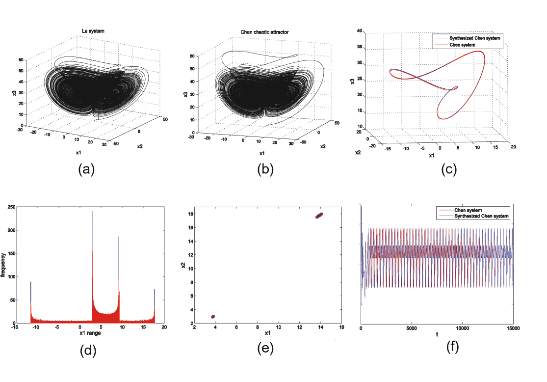
Figure 1: Synthesis of a stable limit cycle for the Chen attractor$,~{}$obtained using the scheme $[1p_{1},2p_{2}]$ with $p_{1}=0.8$ and $p_{2}=0.959$ and $p^{\ast}=0.906$; a) Lü attractor; b) Chen attractor; c) $A^{\ast}$ and $A_{p^{\ast}}$ plotted superimposed; d) Histograms of $A^{\ast}$ and $A_{p^{\ast}}~{}$superimposed; e) Poincaré superimposed sections with plane $x_{3}=28$ of $A^{\ast}$ and $A_{p^{\ast}}.~{}$f) Time series with transients of component $x_{1}$ of $A^{\ast}$ and $A_{p^{\ast}}$ superimposed.

$$\begin{array}[c]{l}repeat\\ ~{}~{}~{}~{}label=\operatorname{rand}(N)\\ ~{}~{}~{}~{}if~{}label=1~{}then\\ ~{}~{}\ ~{}~{}~{}~{}~{}~{}~{}integrate~{}(\ref{ivp general})~{}with~{}p=p_{1}\\ ~{}~{}~{}~{}~{}~{}~{}~{}~{}~{}inc(m_{1}^{{}^{\prime}})\\ ~{}~{}~{}~{}if~{}label=2~{}then\\ ~{}~{}~{}~{}~{}~{}~{}~{}~{}~{}integrate~{}(\ref{ivp general})~{}with~{}p=p_{2}\\ ~{}~{}~{}~{}\ ~{}~{}~{}~{}~{}inc(m_{2}^{{}^{\prime}})\\ ~{}~{}~{}~{}~{}\ldots\\ ~{}~{}~{}~{}if~{}label=N~{}then\\ ~{}~{}~{}~{}~{}~{}~{}~{}~{}~{}integrate~{}(\ref{ivp general})~{}with~{}p=p_{N}\\ ~{}\ ~{}~{}\ ~{}~{}~{}~{}~{}inc(m_{N}^{{}^{\prime}})\\ ~{}~{}~{}~{}~{}t=t+h\\ until~{}t\geq T_{\max}\end{array}$$ (7)

Figure 2: Random SA algorithm.

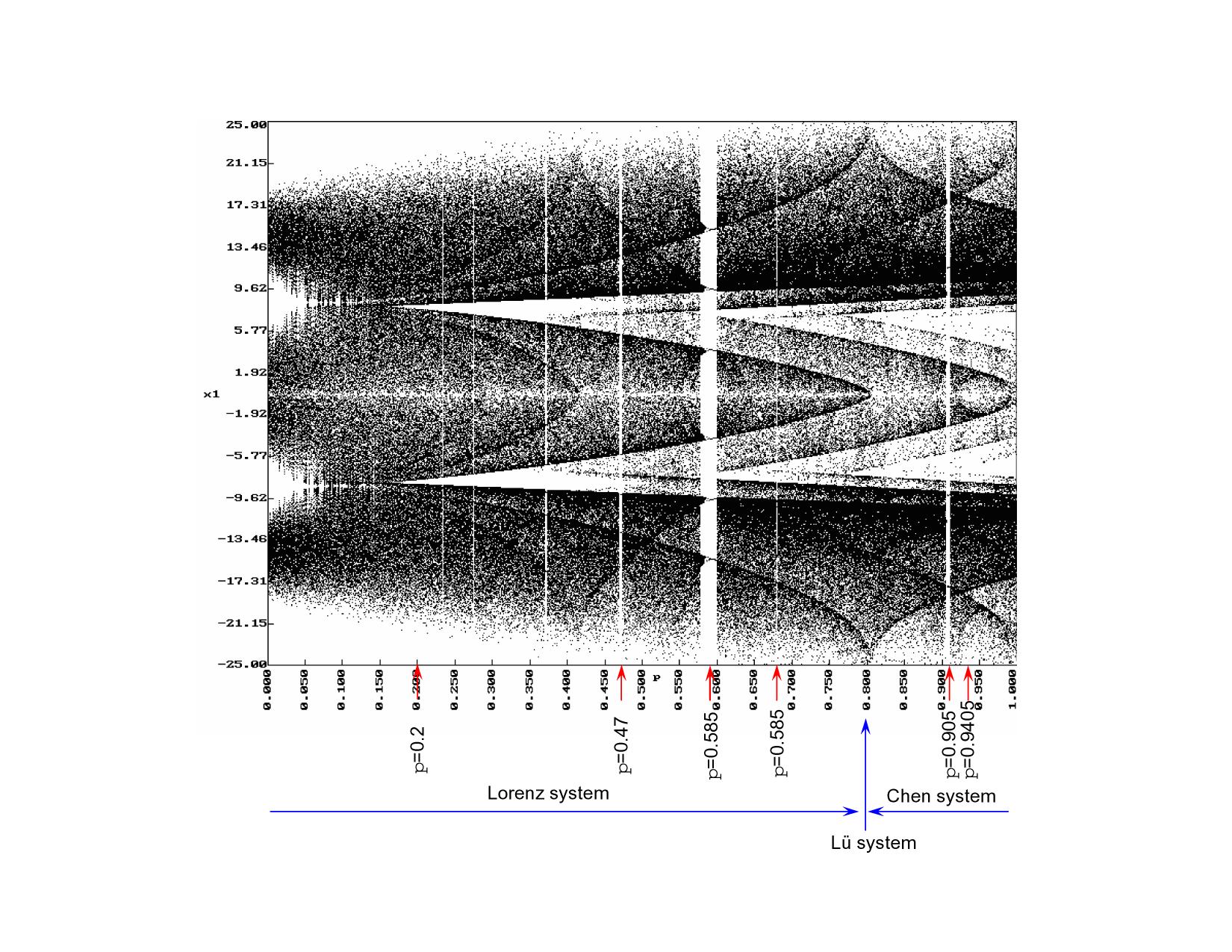
Figure 3: Bifurcation diagram for the Lü system.

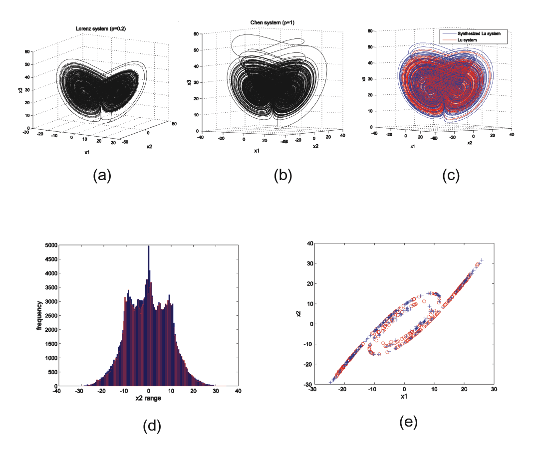
Figure 4: The synthesized Lü attractor obtained with scheme $[1p_{1},3p_{2}]$ for $p_{1}=0.2,$ $p_{2}=1$; a) $A_{p_{1}}$; b) $A_{p_{2}};~{}$c) $A^{\ast}$ and $A_{p^{\ast}}$ plotted superimposed; d) Superimposed histograms; e) Superimposed Poincaré sections.

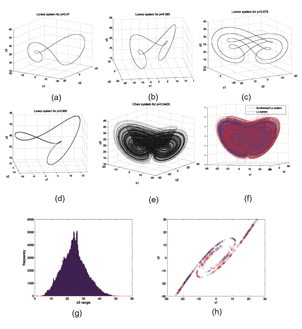
Figure 5: The synthesized Lü attractor obtained with scheme $[1p_{1},$ $1p_{2},1p_{3},1p_{4},4p_{5}]$ for $p_{1}=0.47,~{}p_{2}=0.585,~{}p_{3}=0,678,$ $p_{4}=0.905$ and $p_{5}=0.9405.$ a-e) Attractors $A_{p_{i}},$ $i=1,\ldots,5;$ f) $A^{\ast}$ and $A_{p^{\ast}}~{}$plotted superimposed; g) Superimpose histograms; h) Superimposed Poincaré sections.

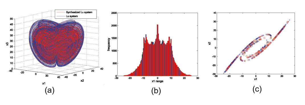
Figure 6: The synthesized Lü attractor obtained with the random scheme in Fig. 1 with uniform distribution of values $p_{1}=0.6$ and$~{}p_{2}=1.$a) Superimposed histograms; b) Superimposed Poincaré sections.

References

- [Lü et al., 2002] Lü, J., Chen, G. Cheng, D. and Celikovsky, S. [2002] ”Bridge the gap between the Lorenz system and the Chen system,” Int. J. Bifurcation and chaos,12, 2917-2926.
- [Chelikovsky & Chen, 2002] Celikovsky, S. and Chen, G. [2002] ”On a generalized Lorenz canonical form of chaotic systems,” Int. J. Bifurcation and Chaos 12, 1789-1812.
- [Lü & Chen, 2002] Lü, J. and Chen, G. [2002] ”A new chaotic attractor coined,” Int. J. Bifurcation and chaos 12, 659-661.
- [Danca et al., 2008] Danca, M.-F., Tang, W. K. S. and Chen, G. [2008] ”A switching scheme for synthesizing attractors of dissipative chaotic systems,” Applied Mathematics and Computations 201, 650-67.
- [Chen & Ueta, 1999] Chen, G. and Ueta, T. [1999] ”Yet another chaotic attractor,” Int. J. Bifurcation and Chaos 9, 1465-1466.
- [Foias & Jolly, 1995] Foias, C. and Jolly, M. S. [1995] ”On the numerical algebraic approximation of global attractors,” Nonlinearity. 8, 295–319.
- [Milnor, 1985] Milnor, J. [1985] ”On the concept of attractor,” Communications in Mathematical Physics 99, 177–195.
- [Danca, 2008] Danca, M.-F. [2008] ”Random parameter-switching synthesis of a class of hyperbolic attractors,” Chaos. 18, 033111.
- [Danca, 2009] Danca, M-F. [2009] ”Finding stable attractors of a class of dissipative dynamical systems by numerical parameter switching,” Dynamical Systems, DOI 10.1080/14689360903401278.
- [Luo et al., 2007] Luo, X., Small, M., Danca, M.-F. and Chen. G. [2007] ”On a dynamical system with multiple chaotic attractors,” Int. J. Bifurcation and Chao 17, 3235-3251.
- [Danca & Kai, 2010] Danca, M.-F. and Diethlem, K. [2010] ”Fractional-order attractors synthesis via parameter switching,” Commun Nonlinear Sci Numer Simulat, doi:10.1016/j.cnsns.2010.01.011, 2019.
- [Falconer, 1990] Falconer, K. [1990] Fractal Geometry, Mathematical Foundations and Applications (John Wiley & Sons, Chichester).