Weak topological insulator with protected gapless helical states

Abstract

A workable model for describing dislocation lines introduced into a three-dimensional topological insulator is proposed. We show how fragile surface Dirac cones of a weak topological insulator evolve into protected gapless helical modes confined to the vicinity of dislocation line. It is demonstrated that surface Dirac cones of a topological insulator (either strong or weak) acquire a finite-size energy gap, when the surface is deformed into a cylinder penetrating the otherwise surface-less system. We show that when a dislocation with a non-trivial Burgers vector is introduced, the finite-size energy gap play the role of stabilizing the one-dimensional gapless states.

I Introduction

The topological insulator has become one of the cutting-edge paradigms of the condensed-matter community since the last couple of years. Moore (2010); Hasan and Kane (2010); Qi and Zhang (2010) Especially highlighted is the $Z_{2}$ topological insulator, Kane and Mele (2005a) which has a band gap generated by spin-orbit coupling, and preserves time-reversal symmetry. Though the idea of $Z_{2}$ topological insulator stems from the two-dimensional (2D) quantum spin Hall effect, Kane and Mele (2005b) its three-dimensional (3D) counterpart has given a stronger impact on material science, leading, in particular, to the reclassifying of thermo-conducting layered crystals such as Bi₂Se₃ and Bi₂Te₃ as ”strong” topological insulators. Hasan and Kane (2010) In contrast to its 2D analogue, the 3D $Z_{2}$ topological insulator has both weak and strong phases. Fu et al. (2007); Fu and Kane (2007) A strong (weak) topological insulator bears an odd (even) number of surface Dirac cones when it is in contact with the vacuum, and is characterized by a $Z_{2}$-invariant $\nu_{0}=1$ ($\nu_{0}=0$). Full characterization of a 3D $Z_{2}$ topological insulator requires, however, a set of in total four $Z_{2}$ numbers: $(\nu_{0};\nu_{1}\nu_{2}\nu_{3})$.

In contrast to the topological number $\nu_{0}$ that characterizes a strong topological insulator (STI) and is associated with a protected surface single Dirac cone, other ”weak indices” are generally believed to be nonrobust quantities. On a perfect lattice, this assertion is indeed justified. A recent study, however, on the response of a topological insulator to the introduction of lattice dislocations, Ran et al. (2009) e.g., screw and edge dislocations, suggests that such dislocation lines play the role of a probe for characterizing WTI, in which both strong ($\nu_{0}$) and weak ($\nu_{1}\nu_{2}\nu_{3}$) indices come into play. The authors of Ref. Ran et al. (2009) have shown that both WTI and STI, when twisted by dislocations, accommodate a pair of protected one-dimensional (1D) helical modes. This seems to contradict the common belief that a WTI is not topologically robust. It is also counterintuitive that there always appear an even number, say, two pairs of Dirac cones on the 2D surface of a WTI, whereas along a dislocation the number of protected 1D Dirac cones is at most one. The former is susceptible to disorder, especially to inter-valley scattering by short-range impurities, whereas the latter is spin-protected from scattering by non-magnetic impurities.

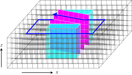
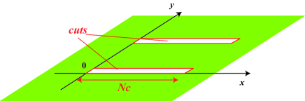
Figure 1: A pair of screw dislocations (upper) with Burgers vector $\bm{b}=(0,0,\pm b)$ inserted between the two cuts (lower). The dislocation line is along the $z$-axis and parallel to the Burgers vector. The system is translationally invariant in the $z$-direction.

The aim of this paper is to resolve the above seemingly opposing points of view on the behavior of WTI on a 2D surface and along a 1D dislocation line. We propose a concrete theoretical model that is intended to interpolate between the two cases. To implement either screw or edge dislocations; see Figs. 1 and 2), we first introduce two cuts extended in parallel with the $z$-axis. For analytic considerations it is more convenient to regard such linear cuts (of width $N_{c}$) as cylindrical punctures (of circumference $s$) penetrating the otherwise surfaceless system. By ”cuts” we mean links on which electron hopping is switched off in the tight-binding description. A pair of screw (edge) dislocations are then introduced around (between) these two cuts. Electrons in the surface states (only such electrons are relevant to transport characteristics) can be seen as a collection of 1D modes that come in pairs (Kramers’ pair), moving up and down the punctures. These electrons also feel the existence of crystal dislocations. The latter plays a role similar to that of an (imaginary) magnetic flux piercing the puncture. The previously mentioned 2D and 1D cases are naturally included within this model as the limit of, respectively, $s\rightarrow\infty$ and $s\rightarrow 0$. We follow the evolution of electronic states along such punctures with a non-trivial lattice distortion as $s$ is varied. It is revealed that the topological stability of protected 1D gapless helical modes stems from a finite-size energy gap associated with the spin Berry phase. The latter has been a subject of much theoretical attention Rosenberg et al. (2010); Zhang and Vishwanath (2010); Bardarson et al. (2010) in the context of peculiar Aharonov-Bohm oscillations observed recently in a system of STI. Peng et al. (2010) The protected gapless modes along dislocation lines have been studied also from the viewpoint of engineering thermo-electric materials. Tretiakov et al. (2010)

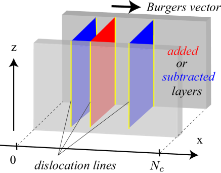
Figure 2: Edge dislocations; a concrete implementation between the two cuts. Here, the Burgers vector $\vec{b}$ is parallel to the $x$-axis; $\vec{b}=(b,0,0)$.

II Model

In the bulk (outside the punctures and away from the dislocation) we consider a lattice version of the following simplified model for 3D $Z_{2}$ topological insulator: Rosenberg and Franz (2010); Rosenberg et al. (2010)

$$H=Ak_{\mu}\gamma_{\mu}+(\Delta-Bk_{\mu}k_{\mu})\gamma_{0}$$ (1)

where repeated indices should be summed over $\mu=1,2,3$. $\gamma$-matrices are chosen, e.g., as,

$$\gamma_{\mu}=\tau_{z}\sigma_{\mu},\ \ \ \gamma_{0}=\tau_{x}$$ (2)

for $\mu=1,2,3$. Then, following the same type of procedure as described in Refs. Imura et al. (2010); Rosenberg and Franz (2010), we place the model on a 3D square lattice of size $N_{x}\times N_{y}\times N_{z}$, and impose, unless stated otherwise a periodic boundary condition in each direction.

Away from the two cuts and dislocations, our tight-binding Hamiltonian reads,

$$H = \sum_{x,y,k_{z}}\big{\{}m(k_{z})|x,y,k_{z}\rangle\langle x,y,k_{z}|$$ (3)

$$+ \big{(}t_{x}|x+1,y,k_{z}\rangle\langle x,y,k_{z}|$$

$$+ t_{y}|x,y+1,k_{z}\rangle\langle x,y,k_{z}|+h.c.\big{)}\big{\}}$$

where

$$m(k_{z}) = A\sin k_{z}\tau_{z}\sigma_{z}+(\Delta-6B+2B\cos k_{z})\tau_{x},$$

$$t_{x} = i{A\over 2}\tau_{z}\sigma_{x}+B\tau_{x},$$

$$t_{y} = i{A\over 2}\tau_{z}\sigma_{y}+B\tau_{x}.$$ (4)

II.1 Cuts

In order to implement a punctured geometry and introduce dislocations on the square lattice, we first deform the punctures into the form of a ”cut” (see the lower panel of FIG. 1) of length $N_{c}$ (its circumference is $s=2N_{c}$). We introduce two cuts, then a pair of screw (Fig. 1) or edge (Fig. 2) dislocations between them. As shown in these figures, here the two cuts are placed along the $z$-axis, and between the two crystal layers: $y=0$ and $y=1$ (as well as between $y=N_{y}/2-1$ and $y=N_{y}/2$). Between these crystal layers hopping is turned off for $x=1,\cdots,N_{c}$. Introduction of these two cuts breaks the discrete translational invariance (crystal periodicity) in the $(x,y)$-plane, whereas it preserves the translational invariance in the $z$-direction, i.e., $k_{z}$ is still a good quantum number. In the following, we will extensively investigate energy spectra: $E=E(k_{z})$ of the system in the presence of screw or edge dislocations.

II.2 Screw vs. edge dislocations

II.2.1 Case of screw dislocations

A pair of screw dislocations can be introduced between the two cuts by dislocating the hopping matrix elements in the region between the two cuts (Figs. 1), i.e., for $y=1,\cdots,N_{y}/2$, say, between the two crystal layers $x=0$ and $x=1$ as

$$t_{x}|x+1,y,z\rangle\langle x,y,z|\rightarrow t_{x}|x+1,y,z-b\rangle\langle x,y,z|.$$ (5)

$b$ measures the strength of the dislocation, i.e., the magnitude of the Burgers vector. This is equivalent to ”twisting” the same hopping matrix elements by a factor $e^{ik_{z}b}$ in the $k_{z}$-diagonalized basis. Kawamura et al. (1982) Note that the cuts and twist structure is translationally invariant in the $z$-direction, and $k_{z}$ is still a good quantum number.

II.2.2 Case of edge dislocations

In the case of (a pair of) edge dislocations with burgers vector $\bm{b}=(\pm b,0,0)$, we suppress $b$ nearest-neighbor hopping amplitudes in the $x$-direction between $x=x_{0}$ and $x=x_{0}+1+b$ and also between the two cuts ($1\leq y\leq Ny/2$), and instead introduce a ”skipping” process,

$$t_{x}|x_{0}+1+b,y,z\rangle\langle x_{0},y,z|,$$ (6)

to the tight-binding Hamiltonian (3).

Table 1: Three distinct topological phases of the square lattice Dirac mode: its low-energy effective Hamiltonian around the $\Gamma$-point is given in Eqs. (1), (2).

		$\delta_{0}$	$\delta_{1}$	$\delta_{2}$	$\delta_{3}$		$(\nu_{0};\nu_{1}\nu_{2}\nu_{3})$	phase
$\Delta/B<0$		$+$	$+$	$+$	$+$		$(0;000)$	trivial
$0<\Delta/B<4$		$-$	$+$	$+$	$+$		$(1;000)$	STI
$4<\Delta/B<8$		$-$	$-$	$+$	$+$		$(0;111)$	WTI
$8<\Delta/B<12$		$-$	$-$	$-$	$+$		$(1;111)$	STI
$12<\Delta/B$		$-$	$-$	$-$	$-$		$(0;000)$	trivial

II.3 Strong vs. weak indices

The 3D topological insulator model we employ has three distinct topological phases as shown in Table 1. Indices $\delta_{0}$, $\delta_{1}$, $\delta_{2}$, $\delta_{3}$ in the Table are parity eigenvalues: $\pm 1$, respectively, at $\Gamma=(0,0,0)$ (for $\delta_{0}$), at three inequivalent but symmetric $X$-points: $(\pi,0,0)$, $(0,\pi,0)$, $(0,0,\pi)$ (for $\delta_{1}$), at three $M$-points: $(0,\pi,\pi)$, $(\pi,0,\pi)$, $(\pi,\pi,0)$ (for $\delta_{2}$) and at $R=(\pi,\pi,\pi)$ (for $\delta_{3}$). The above eight (by distinguishing inequivalent points) symmetry points ($\Gamma$, $X$, $M$ and $R$) are also called time-reversal invariant momenta (TRIM) of the 3D Brillouin zone. These parity eigenvalues are in our model related to the strong and weak indices as,

$$(-1)^{\nu_{0}} = \delta_{0}\delta_{1}\delta_{1}^{\prime}\delta_{1}^{\prime\prime}\delta_{2}\delta_{2}^{\prime}\delta_{2}^{\prime\prime}\delta_{3}=\delta_{0}\delta_{1}^{3}\delta_{2}^{3}\delta_{3},$$ (7)

$$(-1)^{\nu_{1}} = \delta_{1}\delta_{2}^{\prime}\delta_{2}^{\prime\prime}\delta_{3}=\delta_{1}\delta_{2}^{2}\delta_{3},$$ (8)

$$(-1)^{\nu_{2}} = \delta_{1}^{\prime}\delta_{2}\delta_{2}^{\prime\prime}\delta_{3}=\delta_{1}\delta_{2}^{2}\delta_{3},$$ (9)

$$(-1)^{\nu_{3}} = \delta_{1}^{\prime\prime}\delta_{2}\delta_{2}^{\prime}\delta_{3}=\delta_{1}\delta_{2}^{2}\delta_{3}.$$ (10)

Here, we have distinguished, for later convenience, three $\delta_{2}$’s and $\delta_{3}$’s at symmetric but inequivalent TRIM (the value of these $\delta$’s are identical in our model with high symmetry; as for definitions of these $\delta$’s, see Fig. 8).

In the following, we focus on the WTI phase: $4<\Delta/B<8$, and study how a protected 1D helical pair arises from a topologically fragile surface of a WTI.

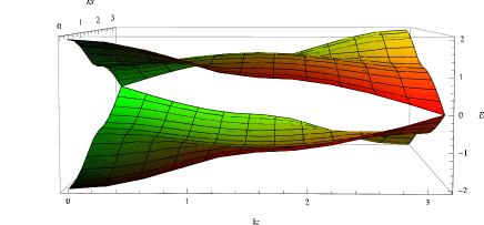
Figure 3: Calculated spectrum of surface Dirac cones. in the WTI phase ($\Delta/B=6$, $A=B=1$). Periodic boundary condition in the $y$-direction is relaxed; the system forms a slab, or a torus of finite thickness. The two Dirac cones are located at TRIM: $(\pi,0)$ and $(0,\pi)$.

III Energy spectrum of WTI in the presence of punctures and dislocation lines

A WTI has an even number of Dirac cones on its surface as depicted in Fig. 3. Here, the surface is chosen normal to the $y$-axis, i.e., a WTI occupying the half space $y<0$ is in contact with the vacuum occupying the remaining half at the $y=0$ surface. The two Dirac cones are located at two TRIM’s: $(0,\pi)$ and $(\pi,0)$ in the surface coordinates $(k_{z},k_{x})$.

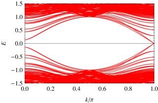
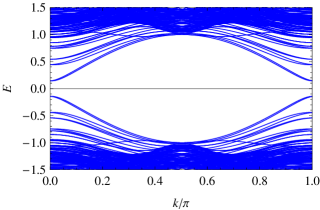
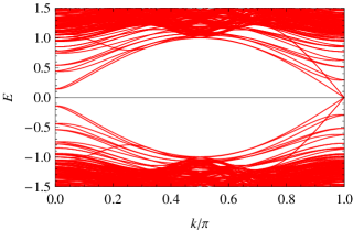
Figure 4: Energy spectrum $E(k)$ of WTI ($\Delta/B=6$) in the presence of screw dislocations. Here, the 1D momentum $k$ is chosen to be along the cuts; $k=k_{z}$. The Burgers vectors are gives as $\vec{b}=(0,0,\pm b)$ with $b=0$ (dislocation is absent), $b=1$, $b=2$ and $b=3$ respectively, in the top, second, third and bottom panels. The calculation is done for a system of size, $N_{x}\times N_{y}=16\times 16$, and cut width $N_{c}=8$. The other parameters are set as $A=B=1$.

III.1 Finite-size energy gap of surface Dirac cones on a cylindrical surface

Imagine deforming this flat surface into a cylindrical tube. The tube is further deformed adiabatically into a cut of Fig. 1 and Fig. 2. The two Dirac cones are now projected onto the $k_{z}$-axis, as shown in the Fig. 4. Notice that the two projected Dirac cones at $k_{z}=0$ and $k_{z}=\pi$ have acquired a finite size gap in the upper panel. Note that here the twist is not introduced yet. The appearance of a gap is a rather unexpected phenomenon, if one recalls that carbon nanotubes become either metallic or semiconducting depending on the way a graphene is rolled up into a tube. Saito et al. (1992) Here, a crucial difference from the carbon nanotube case is that the Dirac cone involves a real spin and not a sub-lattice pseudo-spin. The procedure of rolling up a flat surface into a tube introduces a $2\pi$-rotation in spin space along a contour winding around the tube once. Rosenberg et al. (2010); Zhang and Vishwanath (2010); Bardarson et al. (2010) The resulting $-1$ factor changes the boundary condition around the tube from periodic to anti-periodic:

$$e^{i(p_{x}+k^{(0)}_{x})s}\times(-1)=1.$$ (11)

Here, we have decomposed the total crystal momentum of an electron into short- and long-wavelength components:

$$\bm{k}=\bm{k^{(0)}+p}.$$ (12)

$\bm{p}=(p_{x},p_{y})$ refers to the long-wavelength component measured from the Dirac point. The short-wavelength component $\bm{k}^{(0)}=(k^{(0)}_{x},k^{(0)}_{y})$ is, on the other hand, a crystal momentum at the Dirac point, and typically $k^{(0)}_{x}=0,\pi$. Recall here that the circumference $s=2N_{c}$ of the cut is, by its construction, an even integer multiple of the lattice constant, since the cut is made by disconnecting $N_{c}$ links of an otherwise locally perfect crystal. This signifies that

$$e^{ik^{(0)}_{x}s}=1$$ (13)

always holds. As a result, the anti-periodicity of the boundary condition (11) must be taken care of solely by the long-wavelength part of the crystal momentum, and eliminates, as seen e.g. in the spectrum of Fig. 4 (top panel), states on the line $p_{x}=0$ crossing the very bottom of a Dirac cone. Low-energy states in the same figure consist of $p_{x}=\pm\pi/s$, leading to occurrence of a finite-size gap,

$$\Delta E=2A{\pi\over s}.$$ (14)

in the spectrum.

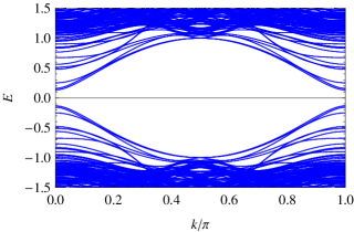
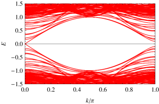
Figure 5: Similar plots as the last two panels of Fig. 4 here in the case of edge dislocations. The Burgers vector is here chosen as $\vec{b}=(\pm b,0,0)$ with $b=2$ and $b=3$, respectively, in the upper and lower panels.

III.2 Screw dislocations

The second panel of Fig. 4 shows, on the other hand, the spectrum when the system is twisted by a pair of screw dislocations with Burgers vector $\vec{b}=(0,0,\pm b)$ where $b=1$. Such a lattice scale deformation modifies the periodicity of the wave function associated with the short-wavelength component of the crystal momentum, i.e., $k^{(0)}_{z}=\pi$ in the present case. Note that the entire effect of a screw dislocation can be concentrated on hopping amplitudes across a single surface, as in Eq. (5). Its influences on the electronic wave function sums up to a phase shift $e^{ik_{z}b}$ on crossing the same surface (here, this is a surface inserted between the two crystal layers $y=0$ and $y=1$). Thus, adding this phase shift to (11) and taking Eq. (13) into account, one finds that the appropriate boundary condition in the presence of a screw dislocation reads,

$$e^{ip_{x}s}\times e^{ik^{(0)}_{z}b}\times(-1)=1.$$ (15)

Note that here a small additional phase factor $e^{ip_{z}b}$ which modifies only gapped solutions with $p_{z}\neq 0$ has been omitted for the sake of clarity. Eq. (15) dictates that only the surface Dirac cone projected onto $k^{(0)}_{z}=\pi$ is susceptible to the change of the magnitude of the Burgers vector, and closes the gap (i.e. the $p_{x}=0$ state is now allowed Zhang et al. (2009)) when $b$ is an odd integer.

Some examples confirming this even/odd feature are shown in Fig. 4. In the last two panels of Fig. 4, one can also observe that Kramers pairs at $k_{z}=0$ exchange their partners as $k_{z}$ evolves up to $k_{z}=\pi$, in accordance with the twisting of boundary condition.

The anti-periodic boundary condition (11), the resulting finite-size gap (14), as well as the twisting of the boundary condition such as Eq. (15) also underlie the origin of the anomalous Aharonov-Bohm oscillations observed recently in Bi₂Se₃ nanoribbbons. Peng et al. (2010) In the Aharonov-Bohm geometry, the twisting of the boundary condition à la Eq. (15) is caused, not by a dislocation, but instead by a magnetic flux tube penetrating the puncture. Rosenberg et al. (2010); Zhang and Vishwanath (2010); Bardarson et al. (2010)

III.3 Edge dislocations

The above argument needs to be modified in the case of an edge dislocation associated with the same dislocation line. Such defects can be introduced e.g., as in Fig. 2, in which dislocations terminate at a cut of finite width similarly to the case of a screw dislocation. The Burgers vector in this implementation is along the $x$-axis, $\bm{b}=(b,0,0)$. Here, $b$ is the number of subtracted (added) layers between the two cuts. Recall that for an edge (screw) dislocation the Burgers vector is perpendicular (parallel) to the dislocation line (parallel to the $z$-axis here). The effect of such an edge dislocation on the electronic wave function can be fully taken into account as a change of the boundary condition (11), i.e., by the replacement: $s\rightarrow s+b$ in the same equation. This leads, when (13) is taken into account, to

$$e^{ip_{x}s}\times e^{ik^{(0)}_{x}b}\times(-1)=1,$$ (16)

i.e., a twisted boundary condition analogous to Eq. (15) but with $k^{(0)}_{z}$ replaced by $k^{(0)}_{x}$. Note that again there is a small additional phase factor $e^{ip_{x}b}$ which appears only when $p_{x}\neq 0$. Eq. (16) dictates, in contrast to Eq. (15), that among the two surface Dirac cones projected onto $k_{z}$-axis, only the one with $p_{x}=\pi$ is susceptible to the presence of edge dislocation, and closes its finite-size gap when $b$ is an odd integer. Two panels of Fig. 5 indeed confirm this even/odd feature in a few non-trivial cases: $b=2,3$. Notice that protected gapless modes appear at $k_{z}=0$ [$b=3$ (odd) case], in contrast to the case of screw dislocation. This is because here the underlying surface Dirac cone responsible for the gap closing is located at $(k_{z},k_{x})=(0,\pi)$, projected naturally to $k_{z}=0$.

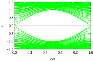
Figure 6: Protected gapless helical modes along a pair of screw dislocations ($b=1$). The spectrum is calculated at $\Delta/B=6$ for two different values of the cut-width $N_{c}$; $N_{c}=0$ (upper) and $N_{c}=16$ (lower). The size of the system is chosen as $N_{x}\times N_{y}=32\times 8$. See the text for discussions.

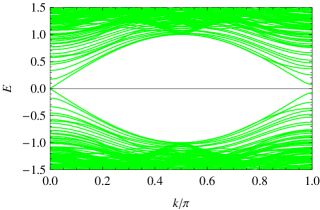
Figure 7: Protected gapless helical modes along a pair of edge dislocations ($b=1$). The spectrum is calculated at $\Delta/B=6$ for two different values of the cut-width $N_{c}$; $N_{c}=1$ (upper) and $N_{c}=16$ (lower). $N_{x}\times N_{y}=32\times 8$.

IV Finite size gap of projected 2D Dirac cones and the protected 1D gapless helical modes

We have seen that 2D surface Dirac cones attains a finite-size mass gap, when the surface is deformed into a tube of finite circumference $s$ (cf. Eqs. (11), (14)). We point out that this observation is the key for understanding the mechanism of how the originally fragile 2D surface Dirac cones of WTI acquires robustness upon the introduction of a dislocation, and transforms into protected 1D gapless helical modes.

In the absence or presence of trivial ($b$: even) dislocations, the finite-size gap evolves continuously into the bulk gap as $s\rightarrow 0$. When $b$ is odd, the same evolution gives robustness to the gapless modes. When the circumference $s$ of the puncture, around which the crystal is dislocated, is finite, the gapless modes are separated from the (gapped) continuum only by an energy of order $A/s$. As the size of the puncture is reduced, only the gapless pairs stay intact, and its unique property that it is topologically protected manifests, making it distinguishable from the rest of the spectrum. Projected Dirac cones without a pair of protected 1D gapless helical modes become indistinguishable from the gapped bulk spectrum.

Fig. 6 (Fig. 7) depicts such an evolution in the presence of screw (edge) dislocations. In the two figures, one can observe, upon reducing the size of the cuts (from lower to upper panels) from $N_{c}=16$ either to $N_{c}=0$ (screw case) or to $N_{c}=1$ (edge case), that the gapless helical pair isolates. Note that in the case of edge dislocations one cannot reduce the cut width smaller than $b$. Note also that in these plots separation between the two cuts is relatively small ($N_{y}/2=4$) in order to take the width of the cut sufficiently large ($N_{c}=16$). For this reason, there appears a finite interference between the ideally gapless counter-propagating modes, each localized in the vicinity of two dislocation lines. Of course, when the size of the cut is finite, the wave function of the gapless mode is extended almost uniformly around the cut. The wave function shows a sharp peak in its amplitude in the vicinity of a dislocation line in the limit $N_{c}\rightarrow 0$ (not shown).

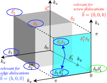
Figure 8: Parity eigenvalues determining both the indices $(\nu_{0};\nu_{1}\nu_{2}\nu_{3})$ and the position of surface Dirac cones on the projected 2D-plane; here chosen as the $(k_{z},k_{x})$-plane. Case 1: screw dislocation [$\vec{b}=(0,0,b)$] — $\delta_{1}^{\prime\prime}\delta_{2}$ and $\delta_{2}^{\prime}\delta_{3}$ occurring at $(k_{z},k_{x})=(\pi,0)$ and $(k_{z},k_{x})=(\pi,\pi)$ are relevant. Case 2: edge dislocation [$\vec{b}=(b,0,0)$] — $\delta_{1}\delta_{2}^{\prime\prime}$ and $\delta_{2}^{\prime}\delta_{3}$ occurring at $(k_{z},k_{x})=(0,\pi)$ and $(k_{z},k_{x})=(\pi,\pi)$ are relevant.

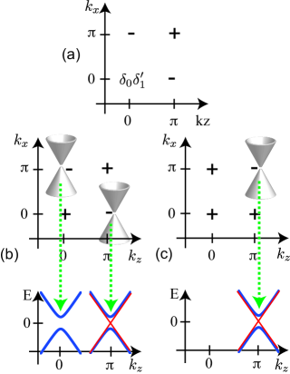
Figure 9: (a) Necessary arrangement of the 2D indices introduced in Fig. 8 for the appearance of protected 1D helical modes along a screw dislocation in the $z$-direction. Only relative signs are relevant. Column (b): WTI example satisfying the condition in (a); $4<\Delta/B<8$. Column (c): STI example satisfying the condition in (a); $8<\Delta/B<12$.

V Relation between weak indices and protected 1D helical modes

What is the relation between the weak indices and condition for the appearance of protected 1D helical modes? A deep connection between these two a priori unrelated quantities becomes manifest when expressing both the weak indices and the latter condition in terms of the parity eigenvalues at the eight bulk TRIM’s, since our system has inversion symmetry. Fu and Kane (2007) The expressions for weak indices in terms of $\delta_{0}$, $\delta_{1}$, $\delta_{2}$ and $\delta_{3}$ were given in Eq. (10). In order to identify the condition for the appearance of protected 1D helical modes in terms of $\delta_{0}$, $\delta_{1}$, $\delta_{2}$, $\delta_{3}$, and $\delta$’s at symmetric but inequivalent points, we project the 3D reciprocal space in which the eight 3D TRIM are defined in two steps; first onto the 2D reciprocal surface on which surface Dirac cones appear, then further onto 1D $k_{z}$-axis on which protected 1D helical modes appear. Fig. 8 shows how the eight parity eigenvalues (among which only four are independent) determine the weak indices, say, $\nu_{3}$, upon projected onto the $(k_{z},k_{x})$-plane. Products of two indices at four 2D TRIM determine the position where surface Dirac cones appear. Fu and Kane (2007)

Fig. 9 shows, on the other hand, that the appearance or disappearance of protected 1D helical modes along a screw dislocation in the $z$-direction is related to a relative sign of indices, $\delta_{1}^{\prime\prime}\delta_{2}$ and $\delta_{2}^{\prime}\delta_{3}$ occurring at $(k_{z},k_{x})=(\pi,0)$ and $(k_{z},k_{x})=(\pi,\pi)$. When these indices have opposite signs,

$$(\delta_{1}^{\prime\prime}\delta_{2})\times(\delta_{2}^{\prime}\delta_{3})=-1,$$ (17)

there appears an odd number of, i.e., a single 2D surface Dirac cone that is projected to $k_{z}=\pi$. This projected Dirac cone acquires a finite-size mass gap that is susceptible to the change of the boundary condition (cf. Eq. (15)) caused by the twisting associated with, e.g., a screw dislocation. The projected Dirac valley features a protected 1D helical modes when $b$ is an odd integer. Notice, on the other hand, that the same combination of parity eigenvalues as Eq. (17) has appeared in Eq. (10) (see also Fig. 8). Thus, ”$\nu_{3}=1$ and $b$ is odd” — (A), is both a necessary and sufficient condition for the appearance of protected 1D gapless helical modes.

The situation is different for an edge dislocation, where the dislocation line is taken to be parallel to the $z$-axis but with a Burgers vector $\bm{b}=(\pm b,0,0)$. In this case, the appearance of protected 1D modes is related to a relative sign of the indices $\delta_{1}\delta_{2}^{\prime\prime}$ and $\delta_{2}^{\prime}\delta_{3}$ occurring at $(k_{z},k_{x})=(0,\pi)$ and $(k_{z},k_{x})=(\pi,\pi)$; see Fig. 8. When these indices have opposite signs, i.e.,

$$(\delta_{1}\delta_{2}^{\prime\prime})\times(\delta_{2}^{\prime}\delta_{3})=-1,$$ (18)

an odd number of surface Dirac cones are susceptible to the change of boundary condition (16) associated with the insertion or subtraction of crystal layers between the two cuts. The same combination of $\delta^{\prime}s$ as Eq. (18) has appeared, in contrast to the previous case, in Eq. (8) (see also Fig. 8). Thus protected 1D gapless modes appear in the present case iff ”$\nu_{1}=1$ and $b$ is odd” — (B).

The above statements (A) and (B) concerning the appearance of protected 1D gapless modes are consistent with the expression,

$$\vec{M}\cdot\vec{b}=\pi\ {\rm mod}\ 2\pi,$$ (19)

which has appeared in Ref. Ran et al. (2009). This formula is a straight-forward generalization of the criteria (A) and (B) to the case of the absence of inversion symmetry. In Eq. (19) the vector $\vec{M}$ is defined as,

$$\vec{M}={1\over 2}(\nu_{1}\vec{G}_{1}+\nu_{2}\vec{G}_{2}+\nu_{3}\vec{G}_{3}),$$ (20)

in terms of reciprocal lattice vectors, $\vec{G}_{1}$, $\vec{G}_{2}$ and $\vec{G}_{3}$. Note that the same formula can be derived by considering winding properties of a Bloch electron in an extended parameter space incorporating the dislocation lines. Teo and Kane (2010)

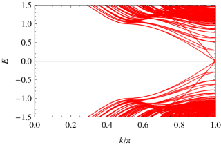
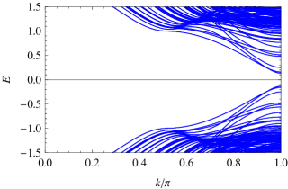
Figure 10: Plots similar to Fig. 4 and Fig. 5 here in the STI phase ($\Delta/B=10$). The upper (lower) panel corresponds to the case of screw (edge) dislocations, $b$ is chosen as, $b=3$ and $b=2$, respectively, in the two cases.

In Fig. 9 (a) the lower-left index $\delta_{0}\delta_{1}$ is irrelevant, since Dirac cones projected onto $k_{z}=0$ is insensitive to the change of boundary condition (cf. Eq. (13)). This means that the dislocation probes only weak indices. Protected 1D gapless helical modes similarly appear both in the WTI and STI phases with the same weak indices (see Fig. 9 columns (b-c)).

Fig. 10 shows STI example on the (dis)appearance of protected gapless modes, both in the screw and edge dislocation cases. Recall that in the WTI phase protected gapless modes along an edge dislocation appear at $k_{z}=0$, whereas here the same protected modes appear at $k_{z}=\pi$, even though the two phases are characterized by the same weak indices; $(\nu_{0};\nu_{1}\nu_{2}\nu_{3})=(0;111)$ [WTI: $4<\Delta/B<8$] and $(\nu_{0};\nu_{1}\nu_{2}\nu_{3})=(1;111)$ [STI: $8<\Delta/B<12$].

VI Conclusions

In this paper, we have addressed the question: how “weak” is a WTI? The existence of protected gapless helical states parasitic to a dislocation line of a WTI seems per se contradictory to the fragility of the even numbers of surface Dirac cones of a WTI. Using a simple model for a topological insulator implemented on a square lattice, we have systematically studied the nature of electronic states in the presence of dislocation lines. In order to resolve the apparent contradiction between the stability of 1D gapless helical modes and the nonrobustness of 2D surface Dirac cones, we have invented and studied a modified variant of the defect-free model in which a dislocation is extended along a cylinder of finite circumference. The unexpected stability of the 1D helical states was identified as an interplay of the finite-size energy gap specific to surface states of a 3D topological insulator and twisting of the boundary condition due to topologically nontrivial geometry. This scenario is closely related to the mechanism of recently observed anomalous Aharonov-Bohm oscillations in a STI of ribbon geometry.