On the connection between the number of nodal domains on quantum graphs and the stability of graph partitions

Abstract.

Courant theorem provides an upper bound for the number of nodal domains of eigenfunctions of a wide class of Laplacian-type operators. In particular, it holds for generic eigenfunctions of quantum graph. The theorem stipulates that, after ordering the eigenvalues as a non decreasing sequence, the number of nodal domains $\nu_{n}$ of the $n$-th eigenfunction satisfies $n\geq\nu_{n}$. Here, we provide a new interpretation for the Courant nodal deficiency $d_{n}=n-\nu_{n}$ in the case of quantum graphs. It equals the Morse index — at a critical point — of an energy functional on a suitably defined space of graph partitions. Thus, the nodal deficiency assumes a previously unknown and profound meaning- it is the number of unstable directions in the vicinity of the critical point corresponding to the $n$-th eigenfunction. To demonstrate this connection, the space of graph partitions and the energy functional are defined and the corresponding critical partitions are studied in detail.

1. Introduction

Nodal domains are defined as the connected components that remain after removing the set of points on which the eigenfunction is zero. They are easy to observe experimentally and their study has a rich history. For a review of the subject see, for example, the collection of articles in [35] or the book [18] (in preparation) and references therein. A cornerstone in the study of nodal domains is Courant’s theorem which states that, after ordering the eigenvalues as a non-decreasing sequence, the number $\nu_{n}$ of nodal domains of the $n$-th eigenfunction is bounded from above by $n$ [13, 14]. It was later proven by Pleijel [31] that for planar problems with Dirichlet boundary conditions, “Courant-sharp” eigenfunctions that satisfy $\nu_{n}=n$ are finite in number, i.e. extremely rare (see also [33]). The sequence of nodal deficiencies, $d_{n}=n-\nu_{n}$ is specific to the particular problem, and it was recently discovered that this sequence encodes information about the geometry of the manifold, much in the same way as the eigenvalue spectrum does [8, 26]. Moreover, the information derived from the nodal count tends to complement the information contained in the spectrum and in certain cases it was shown that isospectral systems can be resolved by their different nodal count sequences[16, 9, 27]. Thus, the question “can one count the shape of a drum” turned out to be a useful paraphrase of Kac’s famous question. The results mentioned above were extended to quantum graphs, where a Pleijel-like theorem does not hold but the intimate link between the nodal count sequence and the graph geometry does exist. [4, 5, 3, 2].

Another link between the spectral and the nodal properties is achieved by studying partitions of the domain into subdomains which minimize a certain energy functional [10, 12, 11]. Recently, Helffer, Hoffmann-Ostenhof and Terracini [24] proved an important result which connects together the notion of a minimal partition and the Courant bound. They consider the Dirichlet problem on a domain $\Omega$. For a partition $P$ of $\Omega$ into subdomains $D_{j}$, $j=1,\ldots,k$, they define the functional

(1.1) $$\Lambda(P)=\max_{1\leq j\leq k}\lambda_{1}(D_{j}),$$

where $\lambda_{1}(D_{j})$ is the first eigenvalue of the Dirichlet Laplacian on $D_{j}$. The minimal partition is defined as the partition on which the minimum of $\Lambda(P)$ over the set of all $k$-partitions is achieved. A partition is bipartite if its subdomains can be labeled with signs $\{+,-\}$ so that neighboring domains have different signs. It was shown in [24] that a minimal partition is bipartite if and only if it corresponds to the eigenfunction that is Courant-sharp.

The result of Helffer et. al. [24] is surprising and even somewhat mysterious. It raises the natural questions: Why only Courant-sharp eigenfunctions appear in the discussion? What about other eigenfunctions, which are, according to Pleijel, the overwhelming majority? In the present work we address these questions in the context of quantum graphs which are defined in Section 1.1. Quantum graphs have the advantage of being simple to analyze without losing the complex spectral features which mark the Laplacian spectra in more general domains. With respect to nodal domains, quantum graphs lie between $d=1$ and higher dimensions. On planar domains, Pleijel’s theorem implies that the nodal deficiency is unbounded from above. However, it was shown in [5] that for quantum graphs the nodal deficiency is bounded from above by the number $\beta$ of independent cycles on the graph. It turns out that this feature makes graphs a very good model to study minimal partitions. We review this and other related results in Section 1.2 below.

The novel element which we introduce here is that the nodal deficiency equals the Morse index of energy functional (1.1) on a suitably defined space of graph partitions. More precisely, we restrict our attention to the so-called equipartitions (see definition 2.1) on which the functional $\Lambda$ becomes differentiable. Under not too restrictive assumptions to be listed below, eigenfunctions are found to correspond to the bipartite critical partitions of the functional $\Lambda$. Furthermore, it turns out that the nodal deficiency of an eigenfunction coincides with the number of unstable directions (Morse index) of the corresponding critical partition. In particular, a minimum has Morse index 0 and therefore corresponds to an eigenfunction of deficiency 0, i.e. a Courant-sharp eigenfunction. Thus, our work extends the result of Helffer, Hoffmann-Ostenhof and Terracini [24] to graphs and goes beyond it by interpreting the nodal deficiency in a new way.

In Section 1.1 we define quantum graphs and their spectrum, in 1.2 we review the nodal count results on graphs. The main results of the paper are presented in Section 2 and proved in subsequent sections. In Section 5 we remove some restrictions we imposed to keep the development simpler and discuss why other restrictions cannot be removed.

1.1. Quantum graphs

In this section we describe the quantum graph which is a metric graph with a Shrödinger-type self-adjoint operator defined on it. Let $\Gamma=(\mathcal{V},\mathcal{E})$ be a graph with vertices $\mathcal{V}=\{v_{j}\}$ and edges $\mathcal{E}=\{e_{j}\}$. The sets $\mathcal{V}$ and $\mathcal{E}$ are required to be finite.

We are interested in metric graphs, i.e. the edges of $\Gamma$ are $1$-dimensional segments with a positive finite length $L_{e}$. On the edge $e=(u,v)$ we assign a coordinate, denoted $x_{e}$, which measures the distance along the edge starting from one of its vertices. A metric graph becomes quantum after being equipped with an additional structure: assignment of a self-adjoint differential operator. This operator will be often called the Hamiltonian. In this paper we study the zeros of the eigenfunctions of the Schrödinger operator

(1.2) $$H\ :\ f(x)\mapsto-\frac{d^{2}f}{dx^{2}}+V(x)f(x),$$

where $x$ is the coordinate along an edge and $V(x)$ is a potential. We will assume that the potential $V(x)$ is bounded and piecewise continuous.

To complete the definition of the operator we need to specify its domain.

Definition 1.1.

We denote by $\widetilde{H}^{2}(\Gamma)$ the space

$$\widetilde{H}^{2}(\Gamma):=\bigoplus_{e\in\mathcal{E}}H^{2}(e),$$

which consists of the functions $f$ on $\Gamma$ that on each edge $e$ belong to the Sobolev space $H^{2}(e)$. The restriction of $f$ to the edge $e$ is denoted by $f_{e}$. The norm in the space $\widetilde{H}^{2}(\Gamma)$ is

$$\|f\|_{\widetilde{H}^{2}(\Gamma)}:=\sum\limits_{e\in\mathcal{E}}\|f_{e}\|_{H^{2}(e)}^{2}.$$

We assume that the domain of the Hamiltonian is a subspace of the Sobolev space $\widetilde{H}^{2}(\Gamma)$. Note that in the definition of $\widetilde{H}^{2}(\Gamma)$ smoothness is enforced along edges only, without any vertex conditions at all. All vertex conditions that lead to the operator (1.2) being self-adjoint have been classified in [28, 19, 30]. The conditions involve the values of the functions $f_{e}$ and their first derivatives at the vertices, both of which are well defined by the standard Sobolev trace theorem. Since the direction is important for the first derivative, we will henceforth adopt the convention that, at an end-vertex of an edge $e$, the derivative is calculated into the edge and away from the vertex.

We will only be interested in the so-called extended $\delta$-type conditions, since they are the only conditions that guarantee continuity of the eigenfunctions, something that is essential if one wants to study changes of sign of the said eigenfunctions.

Definition 1.2.

The domain $\mathcal{H}$ of the operator (1.2) consists of the functions $f\in\widetilde{H}^{2}(\Gamma)$ such that

1. $f$ is continuous on every vertex $v\in\mathcal{V}$:

   $$f_{e_{1}}(v)=f_{e_{2}}(v),$$

   for all edges $e_{1}$ and $e_{2}$ that have $v$ as an endpoint.

2. the derivatives of $f$ at each vertex $v$ satisfy

   (1.3) $$\sum_{e\in\mathcal{E}_{v}}\frac{df}{dx_{e}}(v)=\alpha_{v}f(v),\quad\alpha_{v}\in\mathbb{R},$$

   where $\mathcal{E}_{v}$ is the set of edges incident to $v$.

Sometimes the condition (1.3) is written in a more robust form

(1.4) $$\cos\left(\frac{\varphi_{v}}{2}\right)\sum_{e\in\mathcal{E}_{v}}\frac{df}{dx_{e}}(v)=\sin\left(\frac{\varphi_{v}}{2}\right)f(v),\qquad\varphi_{v}\in(-\pi,\pi],$$

which is also meaningful for infinite values of $\alpha_{v}=\tan\left(\frac{\varphi_{v}}{2}\right)$. Henceforth we will understand $\alpha_{v}=\infty$ as the Dirichlet condition $f(v)=0$. The case $\alpha_{v}=0$ is often referred to as the Neumann-Kirchhoff condition.

The operator (1.2) with the domain $\mathcal{H}$ is self-adjoint for any choice of real $\alpha_{v}$ (including $\alpha_{v}=\infty$). Since we only consider compact graphs, the spectrum is real, discrete and with no accumulation points. We will slightly abuse notation and denote by $\sigma(\Gamma)$ the spectrum of an operator $H$ defined on the graph $\Gamma$. The vertex conditions will usually be clear from the context.

The eigenvalues $\lambda\in\sigma(\Gamma)$ satisfy the equation

(1.5) $$-\frac{d^{2}f}{dx^{2}}+V(x)f(x)=\lambda f(x).$$

It can be shown that under the conditions specified above the operator $H$ is bounded from below [29]. Thus we can number the eigenvalues in an ascending order, starting with $\lambda_{1}$. As the lowest eigenvalue plays an important role in this paper, we adopt the physical terminology and call it the groundstate energy and its corresponding eigenfunction, the groundstate.

The Hamiltonian can also be discussed in terms of its quadratic form [30],

(1.6) $$h[f,f]=\sum_{e}\int|f^{\prime}(x)|^{2}dx+\sum_{e}\int V(x)|f(x)|^{2}dx+\sum_{v}\alpha_{v}|f(v)|^{2},\qquad f\in\widetilde{H}^{1}(\Gamma).$$

As usual, the Dirichlet conditions (if any) are to be introduced directly into the domain of the form rather than included in the last sum of (1.6).

The eigenvalues of the Hamiltonian can be obtained from the quadratic form by applying the Rayleigh-Ritz minimax principle, for instance in the form

(1.7) $$\lambda_{n}=\min_{\dim X=n}\ \max_{f\in X:\,\|f\|=1}h[f,f],$$

where the minimum is taken over all $n$-dimensional subspaces of the domain of the quadratic form.

Finally, we would like to mention that the Neumann-Kirchhoff and Dirichlet vertex conditions play an important role in this paper. Dividing an edge into two parts by introducing a new vertex of degree 2 will have no effect on the spectrum and eigenfunctions if we impose the Neumann condition at the vertex. Indeed, if $\alpha_{v}=0$ and the degree of $v$ is two, equation (1.3) implies that the derivative of a function from the domain of $\mathcal{H}$ is continuous across $v$ and the functions from $H^{2}$-spaces on the sub-edges match up to form a valid function from $H^{2}$-space on the whole edge. On the other hand, imposing the Dirichlet condition is equivalent to cutting the graph at the given point and imposing Dirichlet conditions at the two new vertices of degree 1. We will therefore consider the introduction of such a Dirichlet vertex as a change to the topology of the graph (which might result even in a change of the number of its connected components). Introducing new vertices on a graph is a key element in the present paper.

1.2. Nodal count

The main purpose of this article is to investigate the structural properties of nodal domains of the eigenfunctions of a quantum graph. In this section we define the nodal domains and review some known results.

Nodal domains are the connected components of a graph from which the zero points of a given function have been removed. More precisely, a positive (negative) domain with respect to a function $f$ is a maximal connected subset in $\Gamma$ where $f$ is positive (correspondingly, negative). The total number of positive and negative domains will be called the nodal count of $f$ and denoted by $\nu(f)$. We use $\nu_{n}$ as a shorthand for $\nu(f_{n})$, where $f_{n}$ is the $n$-th eigenfunction of the graph in question. The number of internal zeros of the function $f$ will be denoted by $\mu(f)$ and $\mu_{n}$ is a shorthand for $\mu(f_{n})$. Throughout the manuscript we will assume that the zeros of the function in question do not lie on the vertices of the graph.

The two quantities $\mu$ and $\nu$ are closely related, although, due to the graph topology, the relationship is more complex than on a line, where $\nu=\mu+1$. The topology of the graph comes into play via the first Betti number of $\Gamma$ (hereafter, simply “Betti number”),

(1.8) $$\beta_{\Gamma}=|\mathcal{E}|-|\mathcal{V}|+1.$$

The graph Betti number has several related interpretations. In particular, it counts the number of independent cycles in the graph and gives the minimal number of edges that need to be removed from $\Gamma$ to turn it into a tree. Correspondingly, $\beta_{\Gamma}=0$ if and only if $\Gamma$ is a tree graph, namely if and only if any two vertices of $\Gamma$ are connected by exactly one path.

The graphs considered in this paper are connected. However, since the definition of the nodal domains calls for cutting the graph into several components, it is beneficial to extend equation (1.8) to disconnected graphs. In that case, $\beta_{\Gamma}$ is the sum of Betti numbers of the connected components, leading to

(1.9) $$\beta_{\Gamma}=|\mathcal{E}|-|\mathcal{V}|+k,$$

where $k$ is the number of connected components of $\Gamma$.

Consider a function $f$ which is non-zero on the vertices of $\Gamma$ and has finitely many isolated zeros. Denote the set of zeros by $P=P(f)$ and denote by $\Gamma\setminus P$ the graph obtained by cutting $\Gamma$ at points $P$. Then, by definition of nodal count,

$$\beta_{\Gamma\setminus P}=|\mathcal{E}_{\Gamma\setminus P}|-|\mathcal{V}_{\Gamma\setminus P}|+\nu(f).$$

Since every cut adds 2 new vertices but increases the number of edges by 1 only, we get

(1.10) $$\beta_{\Gamma\setminus P}=|\mathcal{E}_{\Gamma}|-|\mathcal{V}_{\Gamma}|-\mu(f)+\nu(f).$$

Combining equations (1.10) and (1.8) we obtain

(1.11) $$\nu(f)=\mu(f)+1-\left(\beta_{\Gamma}-\beta_{\Gamma\setminus P}\right).$$

In particular, one has the bounds

(1.12) $$\mu-\beta_{\Gamma}+1\leq\nu\leq\mu+1.$$

We now concentrate on the nodal count of the eigenfunctions of the graph. According to the well known ODE theorem by Sturm [36, 37, 25], the zeros of the $n$-th eigenfunction of the operator of type (1.2) on an interval divide the interval into $n$ nodal domains. By contrast, in the corresponding question in $\mathbb{R}^{d}$, $d\geq 2$, only an upper bound is possible, given by the Courant’s nodal line theorem [14], $\nu_{n}\leq n$. In a series of papers [1, 32, 17, 34, 5], it was established that a generic eigenfunction of a quantum graph satisfies both an upper and a lower bound. Namely, let $\lambda_{n}$ be a simple eigenvalue of the Schrödinger operator (1.2), on a graph $\Gamma$ and its eigenfunction $f^{(n)}$ be non-zero at all vertices of $\Gamma$. Then

(1.13) $$n-\beta_{\Gamma}\leq\nu_{n}\leq n.$$

In fact, a simple modification in the proof of the lower bound [5] improves the bound to

(1.14) $$n-\left(\beta_{\Gamma}-\beta_{\Gamma\setminus P}\right)\leq\nu_{n}\leq n.$$

Using formula (1.11) we have a similar formula for the number of zeros,

(1.15) $$n-1\leq\mu_{n}\leq n-1+\left(\beta_{\Gamma}-\beta_{\Gamma\setminus P}\right),$$

or a simpler but weaker version

(1.16) $$n-1\leq\mu_{n}\leq n-1+\beta_{\Gamma}.$$

The conditions for the validity of the above inequalities will be imposed in the present article as well, thus we give them a name.

Definition 1.3.

An eigenfunction $f_{n}$ of a graph $\Gamma$ is called proper if it is non-zero on vertices of $\Gamma$ and the corresponding eigenvalue $\lambda_{n}$ is simple.

Finally we would like to mention that, unlike the $\mathbb{R}^{d}$ case, even the upper bound $\nu_{n}\leq n$ is in general not valid for improper eigenfunctions on quantum graphs.

2. The main results

In the previous section we reviewed the known results on the number of zeros of the $n$-th eigenfunction of a quantum graph. The aim of this paper is to investigate the qualitative features of the $n$-th zero set. The question that should be kept in mind is: given a set of points on the graph, is there an eigenfunction that is zero at precisely these points?

Definition 2.1.

Let $\Gamma$ be a quantum graph.

1. A partition vertex on $\Gamma$ is a new vertex being introduced on an edge of $\Gamma$. The partition vertex is called proper if it is located in the interior of an edge, that is not at an existing vertex of $\Gamma$. Otherwise, we call it an improper partition vertex.

2. An $m$-partition of $\Gamma$ is a set of $m$ partition vertices on the graph. The partition is proper if all of its vertices are proper. Otherwise, we call it an improper partition. The set of all proper $m$-partitions of $\Gamma$ is denoted by $\mathcal{P}_{m}\left(\Gamma\right)$.

Remark 2.2.

An eigenfunction on a generic graph is expected to be non-zero on the vertices of the graph (see [15] for a related result in a special case). Thus improper partitions are not relevant for the study of eigenfunctions on a generic graph. In section 5 we will discuss some pathological aspects of improper partitions, and point out why our restrictions cannot be relaxed. In the rest of the manuscript a partition would always mean a proper one.

Remark 2.3.

The partition $P\in\mathcal{P}_{m}\left(\Gamma\right)$ should be understood as a candidate for the zero set of an eigenfunction. As mentioned in section 1.1, imposing Dirichlet vertex conditions at the partition vertices of $P$ separates $\Gamma$ into several subgraphs, which we denote by $\left\{\Gamma_{j}\right\}$, and call the partition’s subgraphs or connected components. The number of partition components is denoted by $\nu(P)$ and is related to the number of partition points $\mu(P)\equiv m$ via equation (1.11). We chose the number of points $m$ to act as the size of the partition to simplify the subsequent notation. Making the other possible choice, $m:=\nu(P)$, would result in only minor changes to the proof and will have almost no effect on the final result. We note that in dimensions higher than 1, the “number of zeros” concept is no longer available, and the “number of components” therefore acts as the size of the partition.

In the definition of nodal domains in section 1.2 we distinguished positive and negative domains. If an eigenfunction is proper it must change sign at every zero, thus two neighboring domains must have different sign. This motivates the following definition.

Definition 2.4.

The partition $P\in\mathcal{P}_{m}\left(\Gamma\right)$ is called bipartite if there exists a map from its subgraphs to a sign, $\left\{\Gamma_{j}\right\}\rightarrow\left\{+,-\right\}$, such that neighboring subgraphs are mapped to different signs.

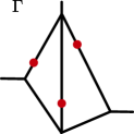
(a)

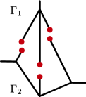
(b)

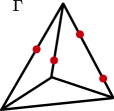
(c)

Figure 2.1. (a) A proper partition $P\in\mathcal{P}_{3}\left(\Gamma\right)$ and (b) its two subgraphs; (c) a non-bipartite partition with $\beta_{\Gamma\setminus P}=1$

We say that a partition $P$ of $\Gamma$ corresponds to a function $f$ on $\Gamma$, or that $f$ corresponds to $P$ if $f$ vanishes exactly at the partition vertices of $P$.

We aim to characterize the partitions that correspond to the eigenfunctions of $H$ on $\Gamma$. As we mentioned already, the partition must be bipartite. Further, observe that for a partition $P$ which corresponds to the $k$-th eigenfunction $f_{k}$ of $\Gamma$ we have for all $j$

$$\lambda_{1}\left(\Gamma_{j}\right)=\lambda_{k}\left(\Gamma\right),$$

where $\lambda_{1}\left(\Gamma_{j}\right)$ is the groundstate eigenvalue of the Hamiltonian $\left.H\right|{}_{\Gamma_{j}}$ restricted to the $j$-th subgraph $\Gamma_{j}$ (with Dirichlet conditions imposed at partition points). This is because the restriction of $f_{k}$ to $\Gamma_{j}$ is an eigenfunction of $\left.H\right|{}_{\Gamma_{j}}$: it satisfies the eigenvalue equation (1.5) and vanishes at the partition points. It must be the groundstate since it does not change sign on $\Gamma_{j}$.

Thus, for a partition to correspond to an eigenfunction, all groundstate energies of the partition’s subgraphs, $\left\{\Gamma_{j}\right\}$, must be equal. This property is referred to in the following definition.

Definition 2.5.

An $m$-partition is an equipartition if all of its subgraphs $\left\{\Gamma_{j}\right\}$ share the same first eigenvalue:

(2.1) $$\lambda_{1}(\Gamma_{j_{1}})=\lambda_{1}(\Gamma_{j_{2}})\qquad\mbox{for all }j_{1},\ j_{2}.$$

The set of all proper equipartitions of $\Gamma$ of size $m$ is denoted $\mathcal{Q}_{m}\left(\Gamma\right)$.

We proceed by defining the following energy functional on $\mathcal{P}_{m}\left(\Gamma\right)$ (compare with similar definition in [12, 24]):

Definition 2.6.

The functional $\Lambda\,:\,\mathcal{P}_{m}\left(\Gamma\right)\rightarrow\mathbb{R}$ is defined by

$$\Lambda\left(P\right):=\max_{j}\lambda_{1}(\Gamma_{j}).$$

The partitions minimizing $\Lambda$ over $\mathcal{P}_{m}\left(\Gamma\right)$ (defined on $d$-dimensional domains) were considered in [12, 24]. However, it is easy to show (as proved for graphs in the next theorem) that any local minimum of $\Lambda$ on $\mathcal{P}_{m}\left(\Gamma\right)$ must be an equipartition. But first we need the notion of proximity for partition. We define the $\varepsilon$-neighborhood of a partition $P\in\mathcal{P}_{m}\left(\Gamma\right)$ to be the set of all the partitions obtained by perturbing the positions of $P$’s partition vertices by a distance smaller than $\varepsilon$.

Theorem 2.7.

Let $P$ be a local minimum of $\Lambda$ on $\mathcal{P}_{m}\left(\Gamma\right)$. Then $P\in\mathcal{Q}_{m}\left(\Gamma\right)$.

Proof of theorem 2.7.

We will prove the theorem by contradiction, by showing that any partition $P\not\in\mathcal{Q}_{m}\left(\Gamma\right)$ can be perturbed to decrease the energy $\Lambda$. The perturbation will be performed upon one partition point at a time, and will use the fact that elongating the edge connected to a degree one vertex with Dirichlet condition decreases the groundstate energy. This follows from the well known Hadamard formula for the derivative of an eigenvalue with respect to the variation of the domain (see [6] for the quantum graph adaptation of the formula).

Let $P\in\mathcal{P}_{m}\left(\Gamma\right)$ be a local minimum of $\Lambda$. Assume that $P$ is not an equipartition. We show that we can perturb the positions of the partition vertices of $P$ in a way which decreases the value of $\Lambda$ and arrive to a contradiction. Let $\left\{\Gamma_{j}\right\}$ be the set of all connected components of $P$. Further, let $\mathcal{I}$ be the set of all $i$ such that $\lambda_{1}\left(\Gamma_{i}\right)=\Lambda\left(P\right)$. In particular, since $P$ is not an equipartition, there exist two neighboring components, $\Gamma_{i}$ and $\Gamma_{j}$, such that $\lambda_{1}\left(\Gamma_{j}\right)<\lambda_{1}\left(\Gamma_{i}\right)=\Lambda\left(P\right)$, that is $i\in\mathcal{I}$ and $j\notin\mathcal{I}$. Let $v$ be a partition vertex which belongs to the common boundary of $\Gamma_{i}$ and $\Gamma_{j}$. We modify $P$ by slightly moving $v$ into $\Gamma_{j}$. Such a perturbation increases $\lambda_{1}\left(\Gamma_{j}\right)$ and decreases $\lambda_{1}\left(\Gamma_{i}\right)$, as discussed above. We use a perturbation small enough such that the relation $\lambda_{1}\left(\Gamma_{j}\right)<\lambda_{1}\left(\Gamma_{i}\right)$ still holds. After performing this perturbation the size of the set $\mathcal{I}$ is reduced by one. We continue perturbing the partition vertices’ positions in the same manner until we exhaust this set. Finally, for the modified partition $P^{\prime}$ we have $\Lambda\left(P^{\prime}\right)<\Lambda\left(P\right)$, which contradicts $P$ being a minimum of $\Lambda$. ∎

Recognizing the significance of equipartitions, we wish to further investigate the energy functional $\Lambda$ restricted to $\mathcal{Q}_{m}\left(\Gamma\right)$. In section 3 we prove the following theorem which describes a parameterization of the set of equipartitions $\mathcal{Q}_{m}\left(\Gamma\right)$.

Theorem 2.8.

Let $\Gamma$ be a finite connected graph with the Betti number $\beta$. Then there exists a number $N$ such that for all $m>N$

1. there is a map $\Phi_{m}$ defined on an open subset of the torus $\mathbb{T}^{\beta}=(-\pi,\pi]^{\beta}$,

2. the map acts bijectively between its domain and the set of proper equipartitions $\mathcal{Q}_{m}\left(\Gamma\right)$.

3. the functional $\Lambda\circ\Phi_{m}$ is smooth.

Remark 2.9.

In the proof of theorem 2.8 the map $\Phi_{m}$ will be constructed explicitly. Furthermore, in theorem 5.1 we will lift the restriction $m>N$ by sacrificing the global structure of the map $\Phi_{m}$.

We may use theorem 2.8 to allow ourselves from now on to identify $m$-equipartitions with elements $\vec{\varphi}=\left(\varphi_{1},\ldots,\varphi_{\beta}\right)\in(-\pi,\pi]^{\beta}$ without mentioning the map. In particular, we can consider the energy functional $\Lambda$ to be defined on the domain of $\Phi_{m}$. This allows us to state the main result of this manuscript:

Theorem 2.10.

Let $\Gamma$ be a finite connected graph. Let $m$ be large enough such that the properties in theorem 2.8 hold.

1. If a bipartite proper equipartition is a critical point of $\Lambda$, then it corresponds to an eigenfunction of $\Gamma$. Conversely, the partition which corresponds to a proper eigenfunction of $\Gamma$ is a critical point of $\Lambda$.

2. If the critical point corresponding to the $n$-th eigenfunction is non-degenerate, the nodal deficiency $d_{n}=n-\nu_{n}$ of the eigenfunction is equal to the Morse index (the number of unstable directions) of the critical point.

Remark 2.11.

Taking 2-dimensional space as an example, a non-degenerate minimum has Morse index 0, a saddle point has index 1 and a maximum index 2. Thus minima correspond to Courant-sharp eigenfunctions, as proved for $\mathbb{R}^{d}$ domains in [24].

The non-degeneracy assumption is introduced to present the theorem in its most elegant form. In fact, in section 4.2 we will prove a certain mixed minimax characterization of the critical points corresponding to the eigenfunction. The nodal deficiency will be equal to the number of maximums taken. We use the non-degeneracy assumption only to go from the minimax to the Morse index. Bypassing this step it is easy to see that even a minimum with a degenerate Hessian still corresponds to a Courant-sharp eigenfunction.

3. Parameterizing the equipartitions

In this section we prove Theorem 2.8 by explicitly constructing the bijection $\Phi_{m}$ between an open subset of the torus $\mathbb{T}^{\beta}=(-\pi,\pi]^{\beta}$ and the set of proper equipartitions $\mathcal{Q}_{m}\left(\Gamma\right)$.

3.1. Description of the map $\Phi_{m}$

Denote $\beta=\beta\left(\Gamma\right)$ and choose $\beta$ edges of $\Gamma$ such that upon their removal we are left with a tree graph. Choose a $\beta$-partition $S$ such that it has one vertex on each of the edges chosen above. This guarantees $\nu\left(S\right)=1$ and that the single connected component of $S$ is a tree (figure 3.1). Denote the partition vertices by $\left\{v_{i}\right\}_{i=1}^{\beta}$ and note that each of them generates two vertices of degree one. We denote these vertices by $\left\{v_{i}^{-},v_{i}^{+}\right\}_{i=1}^{\beta}$ (according to the vertex $v_{i}$ of $S$ which generated them) and equip each pair with the following $\delta$-type conditions:

(3.1) $$\begin{split}\cos\left(\frac{\varphi_{i}}{2}\right)f^{\prime}\left(v_{i}^{-}\right)&=-\sin\left(\frac{\varphi_{i}}{2}\right)\,f\left(v_{i}^{-}\right)\\ \cos\left(\frac{\varphi_{i}}{2}\right)f^{\prime}\left(v_{i}^{+}\right)&=\sin\left(\frac{\varphi_{i}}{2}\right)\,f\left(v_{i}^{+}\right),\end{split}$$

for some $\varphi_{i}\in(-\pi,\pi]$. We denote the resulting tree graph by $\Gamma_{\varphi_{1},\ldots,\varphi_{\beta}}$.

(a)

(b)

Figure 3.1. (a) The graph $\Gamma$ with a partition $P\in\mathcal{P}_{2}\left(\Gamma\right)$.  (b) The resulting tree, $\Gamma_{\varphi_{1},\varphi_{2}}$.

We describe a parameterization of the space of $m$-equipartitions by a map $\Phi_{m}$ from $(-\pi,\pi]^{\beta}$ to the set of equipartitions $\mathcal{Q}_{m}\left(\Gamma\right)$. The action of this map is as follows.

Let $\left(\varphi_{1},\ldots,\varphi_{\beta}\right)\in(-\pi,\pi)^{\beta}$. Examine the eigenspace of the $(m+1)$-th eigenvalue of the tree $\Gamma_{\varphi_{1},\ldots,\varphi_{\beta}}$. If all of its eigenfunctions vanish at some vertex (apart from the vertices with the Dirichlet condition) then the point $\left(\varphi_{1},\ldots,\varphi_{\beta}\right)$ is not in the domain of the definition of the map.

Otherwise, we get by proposition A.1 that the $(m+1)$-th eigenvalue is simple. We can thus apply the nodal bound (1.16) for trees [32, 34] (see also [6] for a short proof) and conclude that the $(m+1)$-th eigenfunction has exactly $m$ zeros on the tree (figure 3.2(a)). The location of the zeros defines a partition $Q\in\mathcal{P}_{m}\left(\Gamma\right)$ on the original graph $\Gamma$, see figure 3.2(b).

We now extend the action of the map $\Phi_{m}$ from $(-\pi,\pi)^{\beta}$ to $(-\pi,\pi]^{\beta}$ by continuity. Indeed, the relevant eigenvalue is simple and thus depends analytically on the parameters $\left(\varphi_{1},\ldots,\varphi_{\beta}\right)$, see [6], since $\varphi_{j}=\pi$ is not particularly different from any other values of $\varphi_{j}$ with respect to the vertex conditions (3.1). However, the varying eigenvalue does not remain the eigenvalue number $m+1$. In general we get the $(m-p+1)$-th eigenvalue, where $p$ is the number of $\varphi_{j}$ that are equal to $\pi$. This is because as $\varphi_{j}\to\pi$, a zero of the $(m+1)$-th eigenfunction is approaching the vertex $v_{j}^{-}$; at $\varphi_{j}=\pi$ this zero becomes the boundary condition at $v_{j}^{-}$ and therefore no longer contributes to the nodal count.

The above extension could have been peformed in the limit $\varphi_{j}\to-\pi$ with identical results. It is thus apparent that $\Phi_{m}$ is actually defined on a $\beta$-torus.

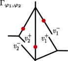
(a)

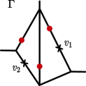
(b)

Figure 3.2. (a) The tree graph $\Gamma_{\varphi_{1},\varphi_{2}}$ and the zeros of its fourth eigenfunction.  (b) The partition $Q=\Phi_{3}\left(\varphi_{1},\varphi_{2}\right)$ on the original graph $\Gamma$ (marked with circles).

Let $\left(\varphi_{1},\ldots,\varphi_{\beta}\right)$ be in the domain of $\Phi_{m}$. Then, as we have already observed in the definition of $\Phi_{m}$, the $(m+1)$-th eigenvalue of the tree $\Gamma_{\varphi_{1},\ldots,\varphi_{\beta}}$ is simple. Therefore (see [6]) it depends analytically on the vertex conditions, that is on the parameters $\left(\varphi_{1},\ldots,\varphi_{\beta}\right)$. In particular, it remains simple in an open ball around the initial $\left(\varphi_{1},\ldots,\varphi_{\beta}\right)$. This proves part 1 of Theorem 2.8.

In order to distinguish between the points of partitions $S$ and $Q$, we call the former section points. We emphasize that the location of the section points, $\left\{v_{i}\right\}_{i=1}^{\beta}$, is fixed and determines the action of the map $\Phi_{m}$. The image of the map, $Q=\Phi_{m}\left(\varphi_{1},\ldots,\varphi_{\beta}\right)$, gives the other set of partition vertices and we claim that $Q$ is an equipartition.

3.2. The minimal value of $m$

Next we make precise our requirement on the number $N$ starting from which the rest of Theorem 2.8 is guaranteed to be valid.

Lemma 3.1.

There exists an $N$ such that for all integers $m>N$ the partition $Q=\Phi_{m}\left(\varphi_{1},\ldots,\varphi_{\beta}\right)$ of $\Gamma$ will have $\beta_{\Gamma\setminus Q}=0$ for every $\left(\varphi_{1},\ldots,\varphi_{\beta}\right)$ in the domain of $\Phi_{m}$.

Proof.

Our proof is constructive: we give an estimate of $N$. However, controlling the Betti number of a resulting partition is hard. Instead we show that for large enough $m$ the partition $Q$ is guaranteed at least one point on every edge of $\Gamma$.

Take an edge $e$ of $\Gamma$ and consider the operator $H$ restricted to this edge with the Dirichlet conditions at the endpoints. Denote the first eigenvalue of $H$ on $e$ by $\lambda_{e}$. For example, if the potential $V\equiv 0$, $\lambda_{e}$ is equal to $\pi/L_{e}$, where $L_{e}$ is the length of $e$. Define

(3.2) $$\lambda_{D}=\max_{e\in\mathcal{E}(\Gamma)}\lambda_{e}.$$

We are now going to prove that: (i) for large enough $m$ the $(m+1)$-th eigenvalue of $\Gamma_{\varphi_{1},\ldots,\varphi_{\beta}}$ is larger than $\lambda_{D}$ for all values of $\left(\varphi_{1},\ldots,\varphi_{\beta}\right)$ and (ii) if the eigenvalue is larger than $\lambda_{D}$, the corresponding eigenfunction of $\Gamma_{\varphi_{1},\ldots,\varphi_{\beta}}$ has a zero on every edge of $\Gamma$. These statements combined would finish the proof of the lemma.

To verify statement (i) we observe that, by Theorem A.4,

$$\lambda_{m-\beta+1}(\Gamma)\leq\lambda_{m+1}\left(\Gamma_{\varphi_{1},\ldots,\varphi_{\beta}}\right).$$

Therefore we only need to find $N$ such that $\lambda_{N-\beta+1}(\Gamma)\geq\lambda_{D}$ and then (i) is satisfied for all $m>N$.

Before we discuss statement (ii) we note that some of the edges of $\Gamma$ are split into two parts in the graph $\Gamma_{\varphi_{1},\ldots,\varphi_{\beta}}$ and some care should be taken with these edges. Let $f$ be an eigenfunction of $\Gamma_{\varphi_{1},\ldots,\varphi_{\beta}}$ with an eigenvalue larger than $\lambda_{D}$. Let $f_{e}$ be the restriction of this function to the edge $e$ of $\Gamma$. If the edge $e$ contains a section point $v_{i}$ then the function $f_{e}$ is likely to be discontinuous at $v_{i}$. To fix this we multiply the function on the right side of $v_{i}$ by a suitable constant (which is $c=f(v_{i}^{-})/f(v_{i}^{+})$). Now we note that due to the special structure of conditions (3.1), the modified function $f_{e}$ is not only continuous at $v_{i}$, but is also continuously differentiable.

The obtained function $f_{e}$ satisfies the differential equation $Hf_{e}=\lambda f_{e}$ on the edge $e$. It also satisfies homogenous boundary conditions at the endpoints $u$ and $v$ of the edge. Namely, $f$ satisfies $f^{\prime}(u)=\alpha_{u}f(u)$ and $f^{\prime}(v)=\alpha_{v}f(v)$, for suitable values of $\alpha_{u}$ and $\alpha_{v}$. Since $\lambda$ is greater than the first Dirichlet eigenvalue of the edge $e$, the monotonicity of the spectrum with respect to the changes of $\alpha$ (see Theorem A.2) implies that $\lambda$ cannot be the first eigenvalue of $H$ on the edge $e$, with the boundary conditions given above. Therefore $f_{e}$ has at least one zero. ∎

Remark 3.2.

For the sake of simplicity of the proof we did not pursue the sharpest estimates. To improve them one can, for example, take the maximum in the definition of $\Lambda$ over a set of edges, removing which turns the graph $\Gamma$ into a tree.

3.3. The map $\Phi_{m}$ produces equipartitions

Now we take $m$ larger than $N$ from Lemma 3.1. Let $f$ be the $(m+1)$-th eigenfunction of $\Gamma_{\varphi_{1},\ldots,\varphi_{\beta}}$. We already observed that $f$ has exactly $m$ nodal points. Hence $f$ corresponds to some partition $Q\in\mathcal{P}_{m}\left(\Gamma\right)$ (figure 3.3(a)). Lemma 3.1 guarantees that $\beta_{\Gamma\setminus Q}=0$ and therefore the subgraphs $\Gamma_{j}$ of the partition are trees. We need to prove that the groundstate energy of every $\Gamma_{j}$ is equal to the same value $\lambda_{m+1}\left(\Gamma_{\varphi_{1},\ldots,\varphi_{\beta}}\right)$. We will do it by considering the restriction of the function $f$ to $\Gamma_{j}$ and modifying it into the groundstate of $\Gamma_{j}$.

The restriction of the function $f$ to $\Gamma_{j}$ satisfies all the vertex conditions on $\Gamma_{j}$ and also satisfies the eigenvalue equation $Hf=\lambda f$ (with $\lambda=\lambda_{m+1}\left(\Gamma_{\varphi_{1},\ldots,\varphi_{\beta}}\right)$) everywhere apart from those section points that happen to lie on $\Gamma_{j}$. At these points the function $f$ is likely to be discontinuous (figure 3.3(b)).

(a)

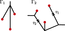
(b)

Figure 3.3. (a) The tree graph $\Gamma_{\varphi_{1},\varphi_{2}}$ and the zeros of its fourth eigenfunction, $f$.  (b) The subgraphs of $Q=\Phi_{3}\left(\varphi_{1},\varphi_{2}\right)$ and the points $v_{1},v_{2}$ at which $f$ is likely to be discontinuous.

We will fix this in a manner similar to the proof of Lemma 3.1. Locate a discontinuity point $v_{i}$. The function satisfies the conditions (3.1) on the left and right of $v_{i}$. They, in particular, imply that $f$ is not zero at $v_{i}^{\pm}$ . Let

$$c=f(v_{i}^{+})/f(v_{i}^{-}).$$

Then, multiplying the function $f$ on the “left” part of the tree $\Gamma_{j}$ (i.e. the one connected to $v_{i}^{+}$) by $c$ we make the resulting function continuous at $v_{i}$. By the special structure of the conditions (3.1) the new function is also continuously differentiable at $v_{i}$. Note that we are able to perform this operation only “on one side” of $v_{i}$ (without affecting $f$ values on the other side) because $\Gamma_{j}$ is a tree and the vertex $v_{i}$ separates it into two components.

However, multiplication by a constant does not spoil any of the properties of $f$ at other locations, namely $f$ satisfying vertex conditions and the eigenvalue equation. By fixing the discontinuities one by one we arrive at a new function $\tilde{f}$ which has sufficient regularity properties to be an eigenfunction of the operator $H$ on $\Gamma_{j}$. Since it has no zeros on $\Gamma_{j}$, it is the groundstate and therefore $\lambda=\lambda_{m+1}\left(\Gamma_{\varphi_{1},\ldots,\varphi_{\beta}}\right)$ is the first eigenvalue of $\Gamma_{j}$. We thus obtain that $Q$ is an equipartition and that

(3.3) $$\Lambda\left(Q\right)=\Lambda\left(\Phi_{m}\left(\varphi_{1},\ldots,\varphi_{\beta}\right)\right)=\lambda_{m+1}\left(\Gamma_{\varphi_{1},\ldots,\varphi_{\beta}}\right).$$

As the eigenvalue $\lambda_{m+1}\left(\Gamma_{\varphi_{1},\ldots,\varphi_{\beta}}\right)$ is analytic with respect to the parameters $\varphi_{1},\ldots,\varphi_{\beta}$, we have also verified part 3 of Theorem 2.8.

3.4. The map $\Phi_{m}$ is bijective

The proof of the bijectivity follows the already established pattern: from an eigenfunction on one graph (either $\Gamma$ or $\Gamma_{\varphi_{1},\ldots,\varphi_{\beta}}$) we construct an eigenfunction on the other by matching the function in a smooth way.

We start by remarking that the map $\Phi_{m}$ is one-to-one. Indeed, in section 3.3, starting from a point $\left(\varphi_{1},\ldots,\varphi_{\beta}\right)$ we constructed the groundstates on all the connected components, $\left\{\Gamma_{j}\right\}$, of the partition $\Phi_{m}\left(\varphi_{1},\ldots,\varphi_{\beta}\right)$. Suppose that another point $(\varphi_{1}^{\prime},\ldots\varphi_{\beta}^{\prime})$ leads to the same partition. Then, for every component $\Gamma_{j}$ of the partition, the same construction leads to a groundstate on $\Gamma_{j}$. But the groundstate is uniquely determined, up to a constant, by $\Gamma_{j}$. And for any section point $v_{i}$ that belongs to $\Gamma_{j}$, the value of $\varphi_{i}$ is uniquely determined by the corresponding groundstate eigenfunction via

(3.4) $$\tan\frac{\varphi_{i}}{2}=\frac{f^{\prime}(v_{i})}{f(v_{i})}.$$

Therefore $\varphi_{i}^{\prime}=\varphi_{i}$ for every section point $i$.

To show that the map is onto we find, for every equipartition $Q$, the point $\left(\varphi_{1},\ldots,\varphi_{\beta}\right)$ that is mapped to it. Let $Q\in\mathcal{Q}_{m}\left(\Gamma\right)$, $m>N$, so that $\beta_{\Gamma\setminus Q}=0$ by Lemma 3.1. Let $\left\{\Gamma_{j}\right\}$ be the subgraphs of the partition $Q$ and $\left\{f_{j}\right\}$ their corresponding normalized groundstates (figure 3.4(a)),

$$\left.H\right|_{\Gamma_{j}\,}f_{j}=\lambda_{1}\left(\Gamma_{j}\right)f_{j}=\Lambda\left(Q\right)f_{j}.$$

As mentioned above, we determine $\varphi_{i}$ from the groundstate of the partition subgraph $\Gamma_{j}\ni v_{i}$ by formula (3.4). To show that the map $\Phi$ sends $\left(\varphi_{1},\ldots,\varphi_{\beta}\right)$ to $Q$ we will construct the $(m+1)$-th eigenfunction of $\Gamma_{\varphi_{1},\ldots,\varphi_{\beta}}$ and verify that its zeros coincide with the partition vertices of $Q$. Define a function $f$ on $\Gamma_{\varphi_{1},\ldots,\varphi_{\beta}}$ by piecing together the groundstates of the subgraphs $\Gamma_{j}$, i.e. $\left.f\right|{}_{\Gamma_{j}}=f_{j}$ (figure 3.4(b)). This function already goes considerable distance towards being an eigenfunction of $\Gamma_{\varphi_{1},\ldots,\varphi_{\beta}}$. Indeed, it satisfies the eigenvalue equation $Hf=\lambda f$ and the vertex conditions on $\Gamma_{\varphi_{1},\ldots,\varphi_{\beta}}$ at every point except the partition vertices of $Q$. At the partition vertices $f$ is continuous (and equal to zero), but might not be differentiable. We remark that the function $f$ will satisfy the conditions at vertices $v_{i}^{\pm}$ because of the special way we defined these conditions — the values $\left(\varphi_{1},\ldots,\varphi_{\beta}\right)$ were especially chosen to fit the function $f$.

(a)

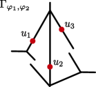
(b)

Figure 3.4. (a) The subgraphs of $Q$, on which the ground states $f_{1},f_{2}$ are taken. (b) The tree graph $\Gamma_{\varphi_{1},\varphi_{2}}$ with the points at which the function $f$ constructed from piecing together $f_{1},f_{2}$ might not be differentiable.

We now modify $f$ so that it becomes continuously differentiable at the partition vertices as well (at the expense of losing the equality $f(v_{i}^{+})=f(v_{i}^{-})$, a property that we do not need on the tree $\Gamma_{\varphi_{1},\ldots,\varphi_{\beta}}$). Choosing a partition vertex $u$ we multiply the function $f$ on the right side of it by the suitably chosen constant

$$c=f^{\prime}(u-0)/f^{\prime}(u+0).\$$

We can perform this operation “on one side” of $u$ because $\Gamma_{\varphi_{1},\ldots,\varphi_{\beta}}$ is a tree and the vertex $u$ separates it into two components. Performing this operation at every partition vertex we will fix all discontinuities but will not break any other properties of $f$. This modified $f$ (with a slight abuse of notation) is an eigenfunction on the tree $\Gamma_{\varphi_{1},\ldots,\varphi_{\beta}}$. It is non-zero on all vertices of the tree and therefore, by Proposition A.1 its eigenvalue is simple. It also has exactly $m$ zeros so, by equation (1.16), it must be the $(m+1)$-th eigenfunction of $\Gamma_{\varphi_{1},\ldots,\varphi_{\beta}}$. This concludes the proof of Theorem 2.8.

4. Proof of theorem 2.10

We begin by recalling that every equipartition $Q\in\mathcal{Q}_{m}\left(\Gamma\right)$ is an image of some point $\left(\varphi_{1},\ldots,\varphi_{\beta}\right)$ under the map $\Phi_{m}$. The action of the map utilizes the $(m+1)$-th eigenfunction of the tree graph $\Gamma_{\varphi_{1},\ldots,\varphi_{\beta}}$. We denote this normalized eigenfunction by $f$ and have

(4.1) $$\Lambda\left(\varphi_{1},\ldots,\varphi_{\beta}\right)=\lambda_{m+1}\left(\Gamma_{\varphi_{1},\ldots,\varphi_{\beta}}\right)=h[f,f],$$

where $h[f,f]$ is the quadratic form (1.6). In what follows we will also use the sesqui-linear form,

$$h[f,g]=\sum_{e}\int f^{\prime}(x)\overline{g^{\prime}(x)}dx+\sum_{e}\int V(x)f(x)\overline{g(x)}dx+\sum_{v}\alpha_{v}f(v)\overline{g(v)}.$$

The sum in the last term above is over all the vertices of $\Gamma_{\varphi_{1},\ldots,\varphi_{\beta}}$ (with the exception of the Dirichlet vertices). In particular, for the vertices $\left\{v_{j}^{-},v_{j}^{+}\right\}_{j=1}^{\beta}$, we have

$$\alpha_{j}^{-}=-\tan\frac{\varphi_{j}}{2}\qquad\qquad\alpha_{j}^{+}=\tan\frac{\varphi_{j}}{2},$$

by the definition of the tree $\Gamma_{\varphi_{1},\ldots,\varphi_{\beta}}$, see (3.1).

4.1. Critical points and eigenfunctions

A critical point is a point where the gradient of $\Lambda\left(\vec{\varphi}\right)$ is equal to zero. We differentiate $\Lambda$ using (4.1),

(4.2) $$\frac{\partial}{\partial\varphi_{j}}\Lambda=\frac{\partial}{\partial\varphi_{j}}\left(h\left[f,f\right]\right)=h_{\varphi_{j}}\left[f,f\right]+h\left[f_{\varphi_{j}},f\right]+h\left[f,f_{\varphi_{j}}\right],$$

where the subscript $\cdot_{\varphi_{j}}$ stands for the partial derivative with respect to $\varphi_{j}$.

We now show that the last two terms in the right-hand side of (4.2) vanish. Recall that $f$ denotes the normalized $(m+1)$-th eigenfunction of $\Gamma_{\varphi_{1},\ldots,\varphi_{\beta}}$. From the normalization of $f$ we get

$$\frac{\partial}{\partial\varphi_{j}}\left\langle f,f\right\rangle=0\qquad\Rightarrow\qquad\left\langle f_{\varphi_{j}},f\right\rangle=0.$$

On the other hand, $f$ is an eigenfunction, therefore (see [6] for details)

(4.3) $$h\left[f_{\varphi_{j}},f\right]=\left\langle f_{\varphi_{j}},Hf\right\rangle=\lambda\left\langle f_{\varphi_{j}},f\right\rangle=0.$$

Since $H$ is self-adjoint, we also have $h\left[f,f_{\varphi_{j}}\right]=0$.

Equation (4.2) now reduces to

(4.4) $$\frac{\partial}{\partial\varphi_{j}}\Lambda =\frac{1}{2\cos^{2}\left(\frac{\varphi_{j}}{2}\right)}\left(\left|f\left(v_{j}^{+}\right)\right|^{2}-\left|f\left(v_{j}^{-}\right)\right|^{2}\right)$$

(4.5) $$=\frac{1}{2\sin^{2}\left(\frac{\varphi_{j}}{2}\right)}\left(\left|f^{\prime}\left(v_{j}^{+}\right)\right|^{2}-\left|f^{\prime}\left(v_{j}^{-}\right)\right|^{2}\right),$$

where, in the last step we used the boundary conditions at $v_{j}^{\pm}$, (3.1). The last expression is useful when $\cos(\varphi_{j}/2)=0$, but in all other cases we will use (4.4).

Now let $\tilde{Q}\in\mathcal{Q}_{m}\left(\Gamma\right)$ be a bipartite proper equipartition which is a critical point of $\Lambda$. Let $\vec{\varphi}=\left(\tilde{\varphi}_{1},\ldots,\tilde{\varphi}_{\beta}\right)$ be the point which is mapped to $\tilde{Q}$ and $\tilde{f}$ the corresponding normalized $(m+1)$-th eigenfunction on the tree $\Gamma_{\tilde{\varphi}_{1},\ldots,\tilde{\varphi}_{\beta}}$. Assume now that $\cos(\varphi_{j}/2)\neq 0$. The condition that $\nabla\Lambda=0$ at $f=\tilde{f}$ implies, via equation (4.4), that

$$\left|\tilde{f}\left(v_{j}^{+}\right)\right|=\left|\tilde{f}\left(v_{j}^{-}\right)\right|$$

for all $j$.

As $\tilde{Q}$ is bipartite, there is an even number of partition points on every cycle. Since the function $\tilde{f}$ changes sign at every partition point, following any cycle from $v_{j}^{+}$ to $v_{j}^{-}$ we deduce that the signs of $\tilde{f}\left(v_{j}^{+}\right)$ and $\tilde{f}\left(v_{j}^{-}\right)$ must agree. Therefore

(4.6) $$\tilde{f}\left(v_{j}^{+}\right)=\tilde{f}\left(v_{j}^{-}\right)\qquad\mbox{ and }\qquad\tilde{f}^{\prime}\left(v_{j}^{+}\right)=-\tilde{f}^{\prime}\left(v_{j}^{-}\right),$$

where we used conditions (3.1) to deduce the second equality from the first. Note that the derivatives are taken in the direction away from the vertices $v_{j}^{\pm}$, therefore the function $\tilde{f}$, if considered on the original graph $\Gamma$ is both continuous and continuously differentiable at all section points $v_{j}$. Since $\tilde{f}$ satisfies the eigenvalue equation, it is an eigenfunction of $\Gamma$.

Note that if $\varphi_{j}=-\pi$ for some $j$, we can similarly deduce equation (4.6) starting with (4.5) and again using bipartiteness.

To prove the second direction of the statement, we start with an eigenfunction of $\Gamma$. It induces an equipartition on $\Gamma$ and the corresponding values of $\tilde{\varphi}_{j}$ can be read off equation (3.1) (see also equation (3.4)). To prove that the point $\left(\tilde{\varphi}_{1},\ldots,\tilde{\varphi}_{\beta}\right)$ is critical, we note that $\tilde{f}$ is smooth at the section points, equation (4.6) is obviously satisfied and (4.4) implies that the gradient is zero.

4.2. A mixed minimax

Let $\tilde{f}$ be the $n$-th eigenfunction on $\Gamma$ with the eigenvalue $\tilde{\lambda}$. Let $\tilde{Q}\leftrightarrow\vec{\varphi}=\left(\tilde{\varphi}_{1},\ldots,\tilde{\varphi}_{\beta}\right)$ be the corresponding $m$-equipartition which, by part 1 is a critical point.

Assume for now that $\tilde{f}$ is non-zero at the section points. Then $\tilde{f}$ is the $(m+1)$-th eigenfunction of $\Gamma_{\tilde{\varphi}_{1},\ldots,\tilde{\varphi}_{\beta}}$, i.e., $\tilde{\lambda}=\lambda_{m+1}\left(\Gamma_{\tilde{\varphi}_{1},\ldots,\tilde{\varphi}_{\beta}}\right)$. We now apply (A.5) to get

(4.7) $$\lambda_{m}\left(\Gamma_{\tilde{\varphi}_{2},\ldots\tilde{\varphi}_{\beta}}\right)\leq\lambda_{m+1}\left(\Gamma_{\varphi_{1},\tilde{\varphi}_{2},\ldots,\tilde{\varphi}_{\beta}}\right)\leq\lambda_{m+1}\left(\Gamma_{\tilde{\varphi}_{2},\ldots\tilde{\varphi}_{\beta}}\right),$$

where $\Gamma_{\tilde{\varphi}_{2},\ldots\tilde{\varphi}_{\beta}}$ is the graph obtained from $\Gamma_{\varphi_{1},\tilde{\varphi}_{2},\ldots,\tilde{\varphi}_{\beta}}$ by gluing the vertices $v_{1}^{-}$ and $v_{1}^{+}$ together into a single vertex $v_{1}$.

The inequalities above hold for all values $\varphi_{1}\in(-\pi,\pi]$. In addition, since we know that $\tilde{f}$ is an eigenfunction of $\Gamma$, it is also an eigenfunction of $\Gamma_{\tilde{\varphi}_{2},\ldots\tilde{\varphi}_{\beta}}$. Therefore, when $\varphi_{1}=\tilde{\varphi}_{1}$ one of the inequalities of (4.7) should become an equality. Namely, there exists some $\sigma_{1}\in\left\{0,1\right\}$, such that

(4.8) $$\lambda_{m+1-\sigma_{1}}\left(\Gamma_{\tilde{\varphi}_{2},\ldots\tilde{\varphi}_{\beta}}\right)=\lambda_{m+1}\left(\Gamma_{\tilde{\varphi}_{1},\tilde{\varphi}_{2},\ldots,\tilde{\varphi}_{\beta}}\right).$$

Carrying the last argument by induction we get that

$$\lambda_{m+1-\sigma_{1}-\sigma_{2}\ldots-\sigma_{\beta}}\left(\Gamma\right)=\lambda_{m+1}\left(\Gamma_{\tilde{\varphi}_{1},\tilde{\varphi}_{2},\ldots,\tilde{\varphi}_{\beta}}\right),$$

for some values $\sigma_{1},\sigma_{2},\ldots,\sigma_{\beta}\in\left\{0,1\right\}$. We now wish to characterize these values.

Consider first the case $\sigma_{1}=0$. Recalling that inequality (4.7) holds for all values $\varphi_{1}\in(-\pi,\pi]$ and combining it with (4.8) allows one to deduce

$$\lambda_{m+1}\left(\Gamma_{\tilde{\varphi}_{2},\ldots\tilde{\varphi}_{\beta}}\right)=\max_{\varphi_{1}\in(-\pi,\pi]}\lambda_{m+1}\left(\Gamma_{\varphi_{1},\tilde{\varphi}_{2},\ldots,\tilde{\varphi}_{\beta}}\right)\qquad\mbox{ if }\sigma_{1}=0.$$

On the other hand, we similarly get

$$\lambda_{m}\left(\Gamma_{\tilde{\varphi}_{2},\ldots\tilde{\varphi}_{\beta}}\right)=\min_{\varphi_{1}\in(-\pi,\pi]}\lambda_{m+1}\left(\Gamma_{\varphi_{1},\tilde{\varphi}_{2},\ldots,\tilde{\varphi}_{\beta}}\right)\qquad\mbox{ if }\sigma_{1}=1.$$

Introducing the notation $\operatorname{opt}_{1}=\min$ and $\operatorname{opt}_{0}=\max$ we can write both equations as

(4.9) $$\lambda_{m+1-\sigma_{1}}\left(\Gamma_{\tilde{\varphi}_{2},\ldots\tilde{\varphi}_{\beta}}\right)=\underset{\varphi_{1}\in(-\pi,\pi]}{\operatorname{opt}_{\sigma_{1}}}\lambda_{m+1}\left(\Gamma_{\varphi_{1},\tilde{\varphi}_{2},\ldots,\tilde{\varphi}_{\beta}}\right).$$

The same reasoning gives

(4.10) $$\lambda_{m+1-\sigma_{1}-\sigma_{2}}\left(\Gamma_{\tilde{\varphi}_{3},\ldots\tilde{\varphi}_{\beta}}\right)=\underset{\varphi_{2}\in(-\pi,\pi]}{\operatorname{opt}_{\sigma_{2}}}\lambda_{m+1-\sigma_{1}}\left(\Gamma_{\varphi_{2},\tilde{\varphi}_{3}\ldots,\tilde{\varphi}_{\beta}}\right).$$

Next we observe that (4.9) holds not only for $\varphi_{2}=\tilde{\varphi}_{2}$ but also in some neighborhood $I_{2}$ of $\tilde{\varphi}_{2}$. In fact, it holds for all values of $\varphi_{2}$ if the value of $\sigma_{1}$ is allowed to depend on $\varphi_{2}$, but we would like to keep it constant. This allows us to substitute (4.9) into the right-hand side of (4.10) and obtain

(4.11) $$\lambda_{m+1-\sigma_{1}-\sigma_{2}}\left(\Gamma_{\tilde{\varphi}_{3},\ldots\tilde{\varphi}_{\beta}}\right)=\underset{\varphi_{2}\in I_{2}}{\operatorname{opt}_{\sigma_{2}}}\underset{\varphi_{1}\in(-\pi,\pi]}{\operatorname{opt}_{\sigma_{1}}}\lambda_{m+1}\left(\Gamma_{\varphi_{1},\varphi_{2},\tilde{\varphi}_{3}\ldots,\tilde{\varphi}_{\beta}}\right).$$

The generalization is now straightforward,

$$\lambda_{m+1-\Sigma}(\Gamma) =\underset{\varphi_{\beta}\in I_{\beta}}{\operatorname{opt}_{\sigma_{\beta}}}\cdots\underset{\varphi_{2}\in I_{2}}{\operatorname{opt}_{\sigma_{2}}}\,\underset{\varphi_{1}\in(-\pi,\pi]}{\operatorname{opt}_{\sigma_{1}}}\lambda_{m+1}\left(\Gamma_{\varphi_{1},\varphi_{2}\ldots,\varphi_{\beta}}\right),$$

(4.12) $$=\underset{\varphi_{\beta}\in I_{\beta}}{\operatorname{opt}_{\sigma_{\beta}}}\cdots\underset{\varphi_{2}\in I_{2}}{\operatorname{opt}_{\sigma_{2}}}\,\underset{\varphi_{1}\in(-\pi,\pi]}{\operatorname{opt}_{\sigma_{1}}}\Lambda\left(\varphi_{1},\ldots,\varphi_{\beta}\right).$$

where $\Sigma=\sigma_{1}+\ldots+\sigma_{\beta}$.

We therefore get that the eigenfunction number $n=m+1-\Sigma$ of $\Gamma$ has $m$ nodal points and therefore $m+1-\left(\beta_{\Gamma}-\beta\left(Q\right)\right)=m+1-\beta$ nodal domains; the latter follows from (1.11) with $\beta_{\Gamma}=\beta$ and $\beta\left(Q\right)=0$. The nodal deficiency of this eigenfunction is therefore $d_{n}=d_{m+1-\Sigma}=\beta-\Sigma$, which equals the number of parameters with respect to which we maximize in (4.12).

We call expression (4.12) the mixed minimax characterization of the eigenvalue since some of the optimizations are minimums and some are maximums. These, in general, do not commute, so the minimax cannot be “unmixed”. Characterization (4.12) is the main result of this subsection.

4.3. Minimax and the Morse index

We end the proof of Theorem 2.10 by showing that if the critical point $\left(\tilde{\varphi}_{1},\ldots,\tilde{\varphi}_{\beta}\right)$ is non-degenerate then its Morse index also equals $\beta-\Sigma$. In other words, we show that the deficiency equals the number of negative eigenvalues of the Hessian of $\Lambda$ at $\left(\tilde{\varphi}_{1},\ldots,\tilde{\varphi}_{\beta}\right)$.

For each value of $\varphi_{2},\ldots,\varphi_{\beta}$ the first optimization of (4.12), is achieved for a certain $\varphi_{1}=\psi_{1}\left(\varphi_{2},\ldots,\varphi_{\beta}\right)$, i.e.

$$\underset{\varphi_{1}\in(-\pi,\pi]}{\operatorname{opt}_{\sigma_{1}}}\Lambda\left(\varphi_{1},\ldots,\varphi_{\beta}\right)=\Lambda\left(\psi_{1}(\varphi_{2},\ldots,\varphi_{\beta}),\varphi_{2},\ldots,\varphi_{\beta}\right).$$

The function $\psi_{1}$ satisfies $\tilde{\varphi}_{1}=\psi_{1}\left(\tilde{\varphi}_{2},\ldots,\tilde{\varphi}_{\beta}\right)$ and defines a manifold $N_{1}\subset(-\pi,\pi]^{\beta}$.

On this manifold, for each value of $\varphi_{3},\ldots,\varphi_{\beta}$, the optimization with respect to $\varphi_{2}$ is achieved at $\varphi_{2}=\psi_{2}\left(\varphi_{3},\ldots,\varphi_{\beta}\right)$, which defines a submanifold $N_{2}\subset N_{1}$. Proceeding in the same manner, we define a sequence $\left\{\psi_{j}\right\}_{j=1}^{\beta}$ of functions and a chain

$$(-\pi,\pi]^{\beta}\supset N_{1}\supset N_{2}\ldots\supset N_{\beta}=\left(\tilde{\varphi}_{1},\ldots,\tilde{\varphi}_{\beta}\right).$$

Wishing to diagonalize the Hessian at the critical point, $\left(\tilde{\varphi}_{1},\ldots,\tilde{\varphi}_{\beta}\right)$, we introduce a new set of variables, $\left(\bar{\varphi}_{1},\ldots,\bar{\varphi}_{\beta}\right)$,

$$\bar{\varphi}_{j}=\varphi_{j}-\psi_{j}\left(\varphi_{j+1},\ldots,\varphi_{\beta}\right),$$

for which we get that

$$N_{j}\subset\left(0,\ldots 0,\bar{\varphi}_{j+1},\ldots,\bar{\varphi}_{\beta}\right).$$

We note that the meaning of the manifolds in the changed variables remains the same: the extremum on $N_{j}$ when varying $\bar{\varphi}_{j+1}$ is achieved when $\bar{\varphi}_{j}=0$, that is on $N_{j+1}$. The extremal property implies that

$$\frac{\partial\Lambda}{\partial\bar{\varphi}_{j}}\Big{|}_{N_{j}}=0.$$

Differentiating this identity with respect to $\bar{\varphi}_{k}$ with $k>j$ (so that we remain on $N_{j}$) we obtain

$$\frac{\partial^{2}\Lambda}{\partial\bar{\varphi}_{k}\partial\bar{\varphi}_{j}}\Big{|}_{N_{j}}=0\qquad k>j.$$

Since the critical point belongs to all $N_{j}$ we conclude that its Hessian is a triangular matrix. In fact, it is diagonal since the Hessian is symmetric. The signs of its diagonal entries at the critical point are known due to the optimization process

(4.13) $$\textrm{sign}\frac{\partial^{2}\Lambda}{\partial\left(\bar{\varphi}_{j}\right)^{2}}\Big{|}_{N_{j}}=2\sigma_{j}-1,$$

where we used the fact that the critical point is non-degenerate. The Morse index of the critical point is independent of the choice of coordinates. We therefore deduce from (4.13) that the Morse index equals to the number of zeros among $\sigma_{j}$, that is $\beta-\Sigma$.

5. Other scenarios

5.1. Low eigenvalues

In the discussion so far we restricted our attention to equipartitions whose parts have no cycles, i.e. $\beta_{\Gamma\setminus Q}=0$. Indeed, Theorems 2.8 and 2.10 ignore all other equipartitions. The justification for this is given by Lemma 3.1, which shows that equipartitions with $\beta_{\Gamma\setminus Q}>0$ do not appear if we restrict ourselves to high enough eigenvalues. However, with some extra work it is possible to extend the treatment to all proper equipartitions.

The parameterization of $\mathcal{Q}_{m}\left(\Gamma\right)$ (for large enough $m$) was done by choosing the location of section points, $\left\{v_{i}\right\}_{i=1}^{\beta}$, which determine the action of the map $\Phi_{m}$. We now take a different approach, which allows us to relax the restriction on the value of $m$ at the cost of sacrificing the global structure of the map $\Phi_{m}$. Given an equipartition $Q\in\mathcal{Q}_{m}\left(\Gamma\right)$, we position the section points depending on $Q$. We recursively add a section point to an edge that contains at least one partition vertex of $Q$ as long as the new section point does not disconnect the graph. It is easy to see that this will result in $k:=\beta_{\Gamma}-\beta_{\Gamma\setminus Q}$ section points, i.e. in general less than before. As a result, each cycle of $\Gamma$ will have a section point if and only if it has a partition vertex of $Q$. We note that if $\beta_{\Gamma}=\beta_{\Gamma\setminus Q}$ we add no section point. One can see that in this case the equipartition $Q$ is isolated.

We can now define the map $\Phi_{m}$ from some open set $D\subset(-\pi,\pi]^{k}$ to some neighborhood of $n$-equipartitions around $Q$. The map acts in the same manner as before (see the discussion preceeding Theorem 2.8). For each $\vec{\varphi}\in D$, $\Phi_{m}\vec{\left(\varphi\right)}$ is the equipartition which corresponds to the zeros of the $(m+1)$-th eigenfunction of $\Gamma_{\vec{\varphi}}$. The validity of the map is proved in the following theorem.

Theorem 5.1.

Let $Q$ be an $n$-equipartition on a finite connected graph $\Gamma$ and let $k=\beta_{\Gamma}-\beta_{\Gamma\setminus Q}$. Denote by $\mathcal{N}(Q)$ the set of proper equipartitions that have the same number of partition points on each edge as $Q$. Then there exists some open set $D\subset(-\pi,\pi]^{k}$ which is bijectively mapped by $\Phi_{m}$ to $\mathcal{N}(Q)$.

Sketch of the proof.

The proof follows the same procedure as the proof of Theorem 2.8. For each partition $Q^{\prime}\in\mathcal{N}(Q)$ we read off the values of $\varphi$ at the section points from the ground states on the corresponding subgraph of the partition. We then reconstruct the eigenfunction on $\Gamma_{\vec{\varphi}}$ using the fact that whenever there is a zero (and thus matching is required) on a cycle of $\Gamma$, this cycle has been cut by a section point (and thus matching is possible).

To see that the obtained eigenfunction of $\Gamma_{\vec{\varphi}}$ is indeed eigenvalue number $m+1$, we use the fact that

$$\beta_{\Gamma_{\vec{\varphi}}}=\beta_{\Gamma\setminus Q^{\prime}},$$

which turns inequality (1.15) into an equation. The eigenfunction in question has $m$ zeros which makes it the eigenfunction number $m+1$.

Openness of the set $D$ follows from continuity of the position of zeros as functions of parameters $\vec{\varphi}$. That is, we can change values of $\vec{\varphi}$ so that the zeros will remain on their corresponding edges. Finally, the injectivity of the map is verified as in the proof of Theorem 2.8, part 2. ∎

Having established the existence of the map $\Phi_{m}$ locally around $Q$, we can use it to define the functional $\Lambda$ on a neighborhood of $Q$. We then obtain a result identical to Theorem 2.10 by following the same proof, as only local properties of $\Lambda$ were used there.

5.2. Improper partitions

In this section we explain the restriction of our results to proper partitions by giving examples of anomalous behavior of improper ones. The unifying feature of our examples is the existence of eigenfunctions vanishing on the vertices of the graph or even on the entire edges. These eigenfunctions arise because of the presence of symmetries in the graphs considered below.

Consider a star graph (see Fig. 5.1) with 3 edges of lengths $l-\varepsilon$, $l$, $l$, where $\varepsilon$ is small. The vertex conditions at the center are Neumann-Kirchhoff (equation (1.3) with $\alpha=0$) and at the outside vertices are Dirichlet.

We inspect the partitions with one nodal point. There are three cases to consider, the point is on the shorter edge, on one of the longer edges and at the central vertex. Denote by $\delta$ the distance of the nodal point to the central vertex. The corresponding values of $\Lambda$ are then

$$\Lambda_{1}=\frac{\pi}{l-\varepsilon-\delta},\qquad\Lambda_{2}=\frac{\pi}{l-\delta},\qquad\Lambda_{3}=\frac{\pi}{l-\varepsilon}.$$

The infimum of the above values as $\delta$ varies is $\pi/l$, but it is not achieved since at $\delta=0$ (nodal point on the longer edge) the functional $\Lambda$ is discontinuous. We note that this problem cannot be cured by seeking minimum over the set of partitions with two parts rather than “partitions by one point”. This approach restores the continuity of $\Lambda$ by removing the offending point from the domain of definition but the infimum is still not achieved. Another anomaly of the above example is that there are no equipartitions with two parts or, equivalently, with one partition point.

(a)

(b)

(c)

Figure 5.1. Three examples of graphs with troublesome (improper) critical partitions.

Consider now a slight modification of the above example, a 3-star graph with edge lengths $l+\varepsilon$, $l$, $l$. In the set of partitions by one point the infimum is again not achieved. The same applies to the set of all partitions into 2 parts. However in the set of partitions into 3 parts the minimum is achieved by the configuration with a nodal point at the center. But this is not an equipartition, violating a would-be analogue of Theorem 2.7.

In a more sophisticated example of a loop of length $l$ with a edge of the same length attached to it, a local maximum among equipartitions with one nodal point is the equipartition with the point at the central vertex. The nearby equipartitions are obtained as the nodal point moves left or right along the loop. It can be shown, however, that the functional $\Lambda$ is not differentiable at the maximum point.

To summarize, the above examples illustrate the necessity of restricting our attention to the generic case (for example, with respect to edge length variation) of proper eigenfunctions.

6. Discussion

We have investigated the connection between zeros of eigenfunctions of a quantum graph and “optimal” partitions of the said graph. This point of view is not new in spectral theory. In a series of papers [21, 23, 22], which culminated in [24], Schrödinger operators on domains in $\mathbb{R}^{2}$ were studied using partitions. Other energy functionals have also been considered, see, for example, [12, 11]. However, it was the minimizers of the maximum functional, equation (3.2) that were shown in [24] to correspond to certain eigenfunctions, namely Courant-sharp ones. However, there is only a finite number of such eigenfunctions for each domain.

We use the same approach to study the connection between partitions and eigenfunctions on quantum graphs. We discover that it is beneficial to restrict the domain of definition of the functional to equipartitions, where the maximum functional becomes differentiable. Upon this restriction, all eigenfunctions of a quantum graph can be characterized as critical points of the energy functional. Furthermore, the Morse index of such a critical point turns out to be equal to the nodal deficiency of the eigenfunction. In the case that the critical point is a minimum, we get that the Morse index is zero and therefore the eigenfunction is Courant-sharp, providing an analogue of the results obtained by Helffer et al [24].

The general nature of our result suggests that analogous theory can be developed for domains in $\mathbb{R}^{d}$ by considering a restriction of the functional $\Lambda$ to the (now infinite-dimensional) set of equipartitions. With the help of the insight gained from the present results, a theorem analogous to Theorem 2.10 has been established in $\mathbb{R}^{d}$ under the assumption that nodal lines (surfaces) do not intersect [7]. A result in the spirit of Theorem 2.10 is also available on discrete graphs (work in progress).

We finish this discussion with a conjecture. The nodal deficiency was determined as the number of maximization in the sequence of $\beta$ operations, see equation (4.12). We conjecture that asymptotically for large $m$ the choice of minimum or maximum become “independent” and “random”, in the sense that the empirical distribution of the deficiencies $d_{n}$ approaches binomial distribution with $p=1/2$ and $n=\beta$.

7. Acknowledgments

The authors are supported by EPSRC (RB: grant number EP/H028803/1, US: grant number EP/G021287), NSF (GB: grant DMS-0907968) and BSF (grant 2006065). The research has been inspired by a talk about the results of [24] given by T. Hoffmann-Ostenhof. We are grateful to Peter Kuchment for suggesting a simpler proof for section 4.3. GB and HR thank Weizmann Institute, where most of the work was done, for warm hospitality. US acknowledges support from the Minerva Center for Nonlinear Physics, the Einstein (Minerva) Center at the Weizmann Institute and the Wales Institute of Mathematical and Computational Sciences (WIMCS).

Appendix A Interlacing theorems for quantum graphs

The following proposition, which forms a part of corollary 5.2 from [6], discusses the connection between manifestations of spectral degeneracy.

Proposition A.1.

Let $T$ be a tree with $\delta$-type conditions at its vertices, with the exclusion that Dirichlet conditions are not allowed on internal vertices. If the eigenvalue $\lambda$ of $T$ has an eigenfunction that is non-zero on all internal vertices of $T$ then $\lambda$ is simple.

We next bring three interlacing theorems from [6], namely theorems 5.1, 5.3 and 5.4.

Theorem A.2.

Let $\Gamma_{\alpha^{\prime}}$ be the graph obtained from the graph $\Gamma_{\alpha}$ by changing the coefficient of the condition at vertex $v$ from $\alpha$ to $\alpha^{\prime}$. If $-\infty<\alpha<\alpha^{\prime}\leq\infty$ (where $\alpha^{\prime}=\infty$ corresponds to the Dirichlet condition), then

(A.1) $$\lambda_{n}(\Gamma_{\alpha})\leq\lambda_{n}(\Gamma_{\alpha^{\prime}})\leq\lambda_{n+1}(\Gamma_{\alpha}).$$

If the eigenvalue $\lambda_{n}(\Gamma_{\alpha^{\prime}})$ is simple and it’s eigenfunction $f$ is such that either $f(v)$ or $\sum f^{\prime}(v)$ is non-zero then the inequalities can be made strict,

(A.2) $$\lambda_{n}(\Gamma_{\alpha})<\lambda_{n}(\Gamma_{\alpha^{\prime}})<\lambda_{n+1}(\Gamma_{\alpha}).$$

Next interlacing theorem is

Theorem A.3.

Let $\Gamma$ be a compact (not necessarily connected) graph. Let $v_{0}$ and $v_{1}$ be vertices of the graph $\Gamma$ endowed with the $\delta$-type conditions, i.e.

$$\begin{cases}f\mbox{ is continuous at }v_{j}\mbox{ and}\\ \sum\limits_{e\in\mathcal{E}_{v_{j}}}\frac{df}{dx_{e}}(v_{j})=\alpha_{j}f(v_{j}),\qquad j=0,1.\end{cases}$$

Arbitrary self-adjoint conditions are allowed at all other vertices of $\Gamma$.

Let $\Gamma^{\prime}$ be the graph obtained from $\Gamma$ by gluing the vertices $v_{0}$ and $v_{1}$ together into a single vertex $v$, so that $\mathcal{E}_{v}=\mathcal{E}_{v_{0}}\cup\mathcal{E}_{v_{1}}$, and endowed with the $\delta$-type condition

(A.3) $$\sum\limits_{e\in\mathcal{E}_{v}}\frac{df}{dx_{e}}(v)=(\alpha_{0}+\alpha_{1})f(v).$$

Then the eigenvalues of the two graphs satisfy the inequalities

(A.4) $$\lambda_{n}(\Gamma)\leq\lambda_{n}(\Gamma^{\prime})\leq\lambda_{m+1}(\Gamma).$$

In the current manuscript we apply the above theorem with $\alpha_{0}=-\alpha_{1}$ and a slight adaptation of (A.2):

(A.5) $$\lambda_{n}(\Gamma^{\prime})\leq\lambda_{m+1}(\Gamma)\leq\lambda_{m+1}(\Gamma^{\prime}).$$

Repeated applications of the theorem above gives the following result, which is a quote of theorem 4.6 from [6].

Theorem A.4.

Let the graph $\Gamma^{\prime}$ be obtained from $\Gamma$ by $k$ identifications, for example by gluing vertices $v_{0},v_{1},\ldots,v_{k}$ into one, or pairwise gluing of $k$ pairs of vertices. Each identification results also in adding the $\alpha_{j}$ parameters in the vertex $\delta$-type conditions, as in (A.3). Then

$$\lambda_{n}(\Gamma)\leq\lambda_{n}(\Gamma^{\prime})\leq\lambda_{n+k}(\Gamma).$$

References

- [1] O. Al-Obeid. On the number of the constant sign zones of the eigenfunctions of a dirichlet problem on a network (graph). Technical report, Voronezh: Voronezh State University, 1992. in Russian, deposited in VINITI 13.04.93, N 938 – B 93. – 8 p.
- [2] R. Band, G. Berkolaiko, and U. Smilansky. Dynamics of nodal points and the nodal count on a family of quantum graphs. arXiv:1008.0505v1 [math-ph], 2010.
- [3] R. Band, I. Oren, and U. Smilansky. Nodal domains on graphs—how to count them and why? In Analysis on graphs and its applications, volume 77 of Proc. Sympos. Pure Math., pages 5–27. Amer. Math. Soc., Providence, RI, 2008.
- [4] R. Band, T. Shapira, and U. Smilansky. Nodal domains on isospectral quantum graphs: the resolution of isospectrality? J. Phys. A, 39(45):13999–14014, 2006.
- [5] G. Berkolaiko. A lower bound for nodal count on discrete and metric graphs. Comm. Math. Phys., 278(3):803–819, 2008.
- [6] G. Berkolaiko and P. Kuchment. Dependence of the spectrum of a quantum graph on vertex conditions and edge lengths. arXiv:1008.0369, 2010.
- [7] G. Berkolaiko, P. Kuchment, and U. Smilansky. Critical partitions and nodal deficiency of billiard eigenfunctions. in preparation, 2011.
- [8] G. Blum, S. Gnutzmann, and U. Smilansky. Nodal domains statistics: A criterion for quantum chaos. Phys. Rev. Lett., 88(11):114101, Mar 2002.
- [9] J. Brüning, D. Klawonn, and C. Puhle. Comment on: “Resolving isospectral ‘drums’ by counting nodal domains” [J. Phys. A 38 (2005), no. 41, 8921–8933] by S. Gnutzmann, U. Smilansky and N. Sondergaard. J. Phys. A, 40(50):15143–15147, 2007.
- [10] D. Bucur, G. Buttazzo, and A. Henrot. Existence results for some optimal partition problems. Adv. Math. Sci. Appl., 8(2):571–579, 1998.
- [11] L. A. Caffarelli and F. H. Lin. An optimal partition problem for eigenvalues. J. Sci. Comput., 31(1-2):5–18, 2007.
- [12] M. Conti, S. Terracini, and G. Verzini. On a class of optimal partition problems related to the Fučík spectrum and to the monotonicity formulae. Calc. Var. Partial Differential Equations, 22(1):45–72, 2005.
- [13] R. Courant. Ein allgemeiner Satz zur Theorie der Eigenfunktione selbstadjungierter Differentialausdrücke. Nach. Ges. Wiss. Göttingen Math.-Phys. Kl., pages 81–84, July 1923.
- [14] R. Courant and D. Hilbert. Methods of mathematical physics. Vol. I. Interscience Publishers, Inc., New York, N.Y., 1953.
- [15] L. Friedlander. Genericity of simple eigenvalues for a metric graph. Israel J. Math., 146:149–156, 2005.
- [16] S. Gnutzmann, U. Smilansky, and N. Sondergaard. Resolving isospectral ‘drums’ by counting nodal domains. J. Phys. A, 38(41):8921–8933, 2005.
- [17] S. Gnutzmann, U. Smilansky, and J. Weber. Nodal counting on quantum graphs. Waves Random Media, 14(1):S61–S73, 2004. Special section on quantum graphs.
- [18] Q. Han and F.-H. Lin. Nodal sets of solutions of elliptic differential equations. book in preparation, 2010.
- [19] M. Harmer. Hermitian symplectic geometry and extension theory. J. Phys. A, 33(50):9193–9203, 2000.
- [20] B. Helffer. On spectral minimal partitions: A survey. Milan Journal of Mathematics, pages 1–16, 2010.
- [21] B. Helffer and T. Hoffmann-Ostenhof. Converse spectral problems for nodal domains, Extended version. Preprint mp_arc 05-343, Sept 2005.
- [22] B. Helffer and T. Hoffmann-Ostenhof. On nodal patterns and spectral optimal partitions. Unpublished notes, Dec. 2005.
- [23] B. Helffer and T. Hoffmann-Ostenhof. Converse spectral problems for nodal domains. Mosc. Math. J., 7:67–84, 2007.
- [24] B. Helffer, T. Hoffmann-Ostenhof, and S. Terracini. Nodal domains and spectral minimal partitions. Ann. Inst. H. Poincaré Anal. Non Linéaire, 26(1):101–138, 2009.
- [25] D. Hinton. Sturm’s 1836 oscillation results: evolution of the theory. In Sturm-Liouville theory, pages 1–27. Birkhäuser, Basel, 2005.
- [26] P. D. Karageorge and U. Smilansky. Counting modal domains on surfaces of revolution. J. Phys. A, 41(20):205102, 26, 2008.
- [27] D. Klawonn. Inverse nodal problems. J. Phys. A, 42(17):175209, 11, 2009.
- [28] V. Kostrykin and R. Schrader. Kirchhoff’s rule for quantum wires. J. Phys. A, 32(4):595–630, 1999.
- [29] P. Kuchment, editor. Quantum graphs and their applications. Special issue of Waves in Random Media, v.14, n.1, 2004.
- [30] P. Kuchment. Quantum graphs. I. Some basic structures. Waves Random Media, 14(1):S107–S128, 2004. Special section on quantum graphs.
- [31] Å. Pleijel. Remarks on Courant’s nodal line theorem. Comm. Pure Appl. Math., 9:543–550, 1956.
- [32] Y. V. Pokornyĭ, V. L. Pryadiev, and A. Al′-Obeĭd. On the oscillation of the spectrum of a boundary value problem on a graph. Mat. Zametki, 60(3):468–470, 1996.
- [33] I. Polterovich. Pleijel’s nodal domain theorem for free membranes. Proc. Amer. Math. Soc., 137(3):1021–1024, 2009.
- [34] P. Schapotschnikow. Eigenvalue and nodal properties on quantum graph trees. Waves in Random and Complex Media, 16:167–78, 2006.
- [35] U. Smilansky and H.-J. Stöckmann, editors. Nodal Patterns in Physics and Mathematics, Wittenberg 2006. The European Physical Journal - Special Topics, vol 145, 2007.
- [36] C. Sturm. Mémoire sur les équations différentielles linéaires du second ordre. J. Math. Pures Appl., 1:106–186, 1836.
- [37] C. Sturm. Mémoire sur une classe d’équations à différences partielles. J. Math. Pures Appl., 1:373–444, 1836.