Localization from Incomplete Noisy Distance Measurements

Abstract

We consider the problem of positioning a cloud of points in the Euclidean space $\mathbb{R}^{d}$, using noisy measurements of a subset of pairwise distances. This task has applications in various areas, such as sensor network localization and reconstruction of protein conformations from NMR measurements. Also, it is closely related to dimensionality reduction problems and manifold learning, where the goal is to learn the underlying global geometry of a data set using local (or partial) metric information. Here we propose a reconstruction algorithm based on semidefinite programming. For a random geometric graph model and uniformly bounded noise, we provide a precise characterization of the algorithm’s performance: In the noiseless case, we find a radius $r_{0}$ beyond which the algorithm reconstructs the exact positions (up to rigid transformations). In the presence of noise, we obtain upper and lower bounds on the reconstruction error that match up to a factor that depends only on the dimension $d$, and the average degree of the nodes in the graph.

1 Introduction

1.1 Problem Statement

Given a set of $n$ nodes in ${\mathbb{R}}^{d}$, the localization problem requires to reconstruct the positions of the nodes from a set of pairwise measurements $\tilde{d}_{ij}$ for $(i,j)\in E\subseteq\{1,\dots,n\}\times\{1,\dots,n\}$. An instance of the problem is therefore given by the graph $G=(V,E)$, $V=\{1,\dots,n\}$, and the vector of distance measurements $\tilde{d}_{ij}$ associated to the edges of this graph.

In this paper we consider the random geometric graph model $G(n,r)=(V,E)$ whereby the $n$ nodes in $V$ are independent and uniformly random in the $d$-dimensional hypercube $[-0.5,0.5]^{d}$, and $E\in V\times V$ is a set of edges that connect the nodes which are close to each other. More specifically we let $(i,j)\in E$ if and only if $d_{ij}=\|x_{i}-x_{j}\|\leq r$. For each edge $(i,j)\in E$, $\tilde{d}_{ij}$ denotes the measured distance between nodes $i$ and $j$. Letting $z_{ij}\equiv\tilde{d}^{2}_{ij}-d^{2}_{ij}$ the measurement error, we will study a “worst case model”, in which the errors $\{z_{ij}\}_{(i,j)\in E}$ are arbitrary but uniformly bounded $|z_{ij}|\leq\Delta$. We propose an algorithm for this problem based on semidefinite programming and provide a rigorous analysis of its performance, focusing in particular on its robustness properties.

Notice that the positions of the nodes can only be determined up to rigid transformations (a combination of rotation, reflection and translation) of the nodes, because the inter point distances are invariant to rigid transformations. For future use, we introduce a formal definition of rigid transformation. Let $X\in{\mathbb{R}}^{n\times d}$ be the matrix whose $i^{th}$ row, $x_{i}^{T}\in{\mathbb{R}}^{d}$, is the coordinate of node $i$. Further, let ${\sf O}(d)$ denote the orthogonal group of $d\times d$ matrices. A set of positions $Y\in{\mathbb{R}}^{n\times d}$ is a rigid transform of $X$, if there exists a $d$-dimensional shift vector $s\in{\mathbb{R}}^{d}$ and an orthogonal matrix $O\in{\sf O}(d)$ such that

$$Y=XO+us^{T}.$$ (1)

Throughout $u\in\mathbb{R}^{n}$ is the all-ones vector. Therefore, $Y$ is obtained as a result of first rotating (and/or reflecting) nodes in position $X$ by matrix $O$ and then shifting by $s$. Also, two position matrices $X$ and $Y$ are called equivalent up to rigid transformation, if there exists $O\in{\sf O}(d)$ and a shift $s\in{\mathbb{R}}^{d}$ such that $Y=XO+us^{T}$. We use the following metric, similar to the one defined in [16], to evaluate the distance between the original position matrix $X\in\mathbb{R}^{n\times d}$ and the estimation $\widehat{X}\in\mathbb{R}^{n\times d}$. Let $L=I-(1/n)uu^{T}$ be the centering matrix . Note that $L$ is an $n\times n$ symmetric matrix of rank $n-1$ which eliminates the contribution of the translation, in the sense that $LX=L(X+us^{T})$ for all $s\in{\mathbb{R}}^{d}$. Furthermore, $LXX^{T}L$ is invariant under rigid transformation and $LXX^{L}=L\widehat{X}\widehat{X}^{T}L$ implies that $X$ and $\widehat{X}$ are equal up to rigid transformation. The metric is defined as

$$d(X,\widehat{X})\equiv\frac{1}{n^{2}}\|LXX^{T}L-L\widehat{X}\widehat{X}^{T}L\|_{1}.$$ (2)

This is a measure of the average reconstruction error per point, when $X$ and $\widehat{X}$ are aligned optimally. To get a better intuition about this metric, consider the case in which all the entries of $LXX^{T}L-L\widehat{X}\widehat{X}^{T}L$ are roughly of the same order. Then

$$d(X,\widehat{X})\approx d_{2}(X,\widehat{X})=\frac{1}{n}\|LXX^{T}L-L\widehat{X}\widehat{X}^{T}L\|_{F}\,.$$

Denote by $Y=\widehat{X}-X$ the estimation error, and assume without loss of generality that both $X$ and $\widehat{X}$ are centered. Then for small $Y$, we have

$$d_{2}(X,\widehat{X})=\frac{1}{n}\|XY^{T}+YX^{T}+YY^{T}\|_{F}\approx\frac{1}{n}\|XY^{T}+YX^{T}\|_{F}$$

$$\stackrel{{\scriptstyle(a)}}{{\geq}}\frac{C}{\sqrt{n}}\|Y\|_{F}=C\left\{\frac{1}{n}\sum_{i=1}^{n}\|\widehat{x}_{i}-x_{i}\|^{2}\right\}^{1/2}\,,$$

where the bound$(a)$ holds with high probability for a suitable constant $C$, if $X$ is distributed according to our model.

Remark. Clearly, connectivity of $G$ is a necessary assumption for the localization problem to be solvable. It is a well known result that the graph $G(n,r)$ is connected w.h.p. if $K_{d}r^{d}>(\log{n}+c_{n})/n$, where $K_{d}$ is the volume of the $d$-dimensional unit ball and $c_{n}\to\infty$ [18]. Vice versa, the graph is disconnected with positive probability if $K_{d}r^{d}\leq(\log{n}+C)/n$ for some constant $C$. Hence, we focus on the regime where $r\geq\alpha(\log{n}/n)^{1/d}$ for some constant $\alpha$. We further notice that, under the random geometric graph model, the configuration of the points is almost surely generic, in the sense that the coordinates do not satisfy any nonzero polynomial equation with integer coefficients.

1.2 Algorithm and main results

The following algorithm uses semidefinite programming (SDP) to solve the localization problem.

Algorithm SDP-based Algorithm for Localization

Input: dimension $d$, distance measurements $\tilde{d_{ij}}$

for $(i,j)\in E$, bound on the measurement noise $\Delta$

Output: estimated coordinates in $\mathbb{R}^{d}$

1: Solve the following SDP problem:

minimize ${\rm Tr}(Q)$     s.t. $\left|\langle M_{ij},Q\rangle-\tilde{d_{ij}}^{2}\right|\leq\Delta,$   $(i,j)\in E$ $Q\succeq\bf{0}$.

2: Compute the best rank-$d$ approximation $U_{d}\Sigma_{d}U_{d}^{T}$ of $Q$

3: Return $\widehat{X}=U_{d}\Sigma_{d}^{1/2}$.

Here $M_{ij}=e_{ij}e_{ij}^{T}\in\mathbb{R}^{n\times n}$, where $e_{ij}\in\mathbb{R}^{n}$ is the vector with $+1$ at $i^{th}$ position, $-1$ at $j^{th}$ position and zero everywhere else. Also, $\langle A,B\rangle\equiv{\rm Tr}(A^{T}B)$. Note that with a slight abuse of notation, the solution of the SDP problem in the first step is denoted by $Q$.

Let $Q_{0}:=XX^{T}$ be the Gram matrix of the node positions, namely $Q_{0,ij}=x_{i}\cdot x_{j}$. A key observation is that $Q_{0}$ is a low rank matrix: ${\rm rank}(Q_{0})\leq d$, and obeys the constraints of the SDP problem. By minimizing ${\rm Tr}(Q)$ in the first step, we promote low-rank solutions $Q$ (since ${\rm Tr}(Q)$ is the sum of the eigenvalues of $Q$). Alternatively, this minimization can be interpreted as setting the center of gravity of $\{x_{1},\dots,x_{n}\}$ to coincide with the origin, thus removing the degeneracy due to translational invariance.

In step 2, the algorithm computes the eigen-decomposition of $Q$ and retains the $d$ largest eigenvalues. This is equivalent to computing the best rank-$d$ approximation of $Q$ in Frobenius norm. The center of gravity of the reconstructed points remains at the origin after this operation.

Our main result provides a characterization of the robustness properties of the SDP-based algorithm. Here and below ‘with high probability (w.h.p.)’ means with probability converging to $1$ as $n\to\infty$ for $d$ fixed.

Theorem 1.1.

Let $\{x_{1},\dots,x_{n}\}$ be $n$ nodes distributed uniformly at random in the hypercube $[-0.5,0.5]^{d}$. Further, assume connectivity radius $r\geq\alpha(\log n/n)^{1/d}$, with $\alpha\geq 10\sqrt{d}$. Then w.h.p., the error distance between the estimate $\widehat{X}$ returned by the SDP-based algorithm and the correct coordinate matrix $X$ is upper bounded as

$$d(X,\widehat{X})\leq C_{1}(nr^{d})^{5}\frac{\Delta}{r^{4}}.$$ (3)

Conversely, w.h.p., there exist adversarial measurement errors $\{z_{ij}\}_{(i,j)\in E}$ such that

$$d(X,\widehat{X})\geq C_{2}\min\{\frac{\Delta}{r^{4}},1\}\,,$$ (4)

Here, $C_{1}$ and $C_{2}$ denote universal constants that depend only on $d$.

The proof of this theorem relies on several technical results of independent interest. First, we will prove a general deterministic error estimate in terms of the condition number of the stress matrix of the graph $G$, see Theorem 5.1. Next we will use probabilistic arguments to control the stress matrix of random geometric graphs, see Theorem 5.2. Finally, we will prove several estimates on the rigidity matrix of $G$, cf. in particular Theorem 6.1. The necessary background in rigidity theory is summarized in Section 2.1.

1.3 Related work

The localization problem and its variants have attracted significant interest over the past years due to their applications in numerous areas, such as sensor network localization [6], NMR spectroscopy [14], and manifold learning [19, 23], to name a few.

Of particular interest to our work are the algorithms proposed for the localization problem [16, 21, 6, 24]. In general, few performance guarantees have been proved for these algorithms, in particular in the presence of noise.

The existing algorithms can be categorized in to two groups. The first group consists of algorithms who try first to estimate the missing distances and then use MDS to find the positions from the reconstructed distance matrix [16, 10]. MDS-MAP [10] and ISOMAP [23] are two well-known examples of this class where the missing entries of the distance matrix are approximated by computing the shortest paths between all pairs of nodes. The algorithms in the second group formulate the localization problem as a non-convex optimization problem and then use different relaxation schemes to solve it. An example of this type is relaxation to an SDP [6, 22, 25, 1, 24]. A crucial assumption in these works is the existence of some anchors among the nodes whose exact positions are known. The SDP is then used to efficiently check whether the graph is uniquely $d$-localizable and to find its unique realization.

Maximum Variance Unfolding (MVU) is an SDP-based algorithm with a very similar flavor as ours [24]. MVU is an approach to solving dimensionality reduction problems using local metric information and is based on the following simple interpretation. Assume $n$ points lying on a low dimensional manifold in a high dimensional ambient space. In order to find a low dimensional representation of this data set, the algorithm attempts to somehow unfold the underlying manifold. To this end, MVU pulls the points apart in the ambient space, maximizing the total sum of their pairwise distances, while respecting the local information. However, to the best of our knowledge, no performance guarantee has been proved for the MVU algorithm.

Given the large number of applications, and computational methods developed in this broad area, the present paper is in many respects a first step. While we focus on a specific model, and a relatively simple algorithm, we expect that the techniques developed here will be applicable to a broader setting, and to a number of algorithms in the same class.

1.4 Organization of the paper

The remainder of this paper is organized as follows. Section 2 is a brief review of some notions in rigidity theory and some properties of $G(n,r)$ which will be useful in this paper. In Section 3, we discuss the implications of Theorem 1.1 in different applications. The proof of Theorem 1.1 (upper bound) is given in Section 4. Sections 5 and 6 contain the proof of two important lemmas used in proving Theorem 1.1. Several technical steps are discussed in Appendices. Finally, We prove Theorem 1.1 (lower bound) in Section 7.

For the reader’s convenience, an overview of the symbols used throughout this paper is given in Table 1 in Appendix N.

2 Preliminaries

2.1 Rigidity Theory

Rigidity theory studies whether a given partial set of pairwise distances $d_{ij}=\|x_{i}-x_{j}\|$ between a finite set of nodes in ${\mathbb{R}}^{d}$ uniquely determine the coordinates of the points up to rigid transformations. This section is a very brief overview of definitions and results in rigidity theory which will be useful in this paper. We refer the interested reader to [13, 2], for a thorough discussion.

A framework $G_{X}$ in ${\mathbb{R}}^{d}$ is an undirected graph $G=(V,E)$ along with a configuration $X\in{\mathbb{R}}^{n\times d}$ which assigns a point $x_{i}\in{\mathbb{R}}^{d}$ to each vertex $i$ of the graph. The edges of $G$ correspond to the distance constraints. In the following, we discuss two important notions, namely Rigidity matrix and Stress matrix. As mentioned above, a crucial part of the proof of Theorem 1.1 consists in establishing some properties of the stress matrix and of the rigidity matrix of the random geometric graph $G(n,r)$.

Rigidity matrix. Consider a motion of the framework with $x_{i}(t)$ being the position vector of point $i$ at time $t$. Any smooth motion that instantaneously preserves the distance $d_{ij}$ must satisfy $\frac{d}{dt}\Arrowvert x_{i}-x_{j}\Arrowvert^{2}=0$ for all edges $(i,j)$. Equivalently,

$$(x_{i}-x_{j})^{T}(\dot{x_{i}}-\dot{x_{j}})=0\quad\forall(i,j)\in E,$$ (5)

where $\dot{x_{i}}$ is the velocity of the $i^{th}$ point. Given a framework $G_{X}\in\mathbb{R}^{d}$, a solution $\dot{X}=[\dot{x}_{1}^{T}\;\dot{x}_{2}^{T}\;\cdots\;\dot{x}_{n}^{T}]^{T}$, with $\dot{x}_{i}\in\mathbb{R}^{d}$, for the linear system of equations (5) is called an infinitesimal motion of the framework $G_{X}$. This linear system of equations consists of $|E|$ equations in $dn$ unknowns and can be written in the matrix form $R_{G}(X)\dot{X}=0$, where $R_{G}(X)$ is called the $|E|\times dn$ rigidity matrix of $G_{X}$.

It is easy to see that for every anti-symmetric matrix $A\in\mathbb{R}^{d\times d}$ and for every vector $b\in\mathbb{R}^{d}$, $\dot{x}_{i}=Ax_{i}+b$ is an infinitesimal motion. Notice that these motions are the derivative of rigid transformations. ($A$ corresponds to orthogonal transformations and $b$ corresponds to translations). Further, these motions span a $d(d+1)/2$ dimensional subspace of ${\mathbb{R}}^{dn}$, accounting $d(d-1)/2$ degrees of freedom for orthogonal transformations (corresponding to the choice of $A$), and $d$ degrees of freedom for translations (corresponding to the choice of $b$). Hence, dim $\textrm{Ker}(R_{G}(X))\geq d(d+1)/2$. A framework is said to be infinitesimally rigid if dim $\textrm{Ker}(R_{G}(X))=d(d+1)/2$.

Stress matrix. A stress for a framework $G_{X}$ is an assignment of scalars $\omega_{ij}$ to the edges such that for each $i\in V$,

$$\sum_{j:(i,j)\in E}\omega_{ij}(x_{i}-x_{j})=(\sum_{j:(i,j)\in E}\omega_{ij})x_{i}-\sum_{j:(i,j)\in E}\omega_{ij}x_{j}=0.$$

A stress vector can be rearranged into an $n\times n$ symmetric matrix $\Omega$ , known as the stress matrix, such that for $i\neq j$, the $(i,j)$ entry of $\Omega$ is $\Omega_{ij}=-\omega_{ij}$, and the diagonal entries for $(i,i)$ are $\Omega_{ii}=\sum_{j:j\neq i}\omega_{ij}$. Since all the coordinate vectors of the configuration as well as the all-ones vector are in the null space of $\Omega$, the rank of the stress matrix for generic configurations is at most $n-d-1$.

There is an important relation between stress matrices of a framework and the notion of global rigidity. A framework $G_{X}$ is said to be globally rigid in $\mathbb{R}^{d}$ if all frameworks in $\mathbb{R}^{d}$ with the same set of edge lengths are congruent to $G_{X}$, i.e. are a rigid transformation of $G_{X}$. Further, a framework $G_{X}$ is generically globally rigid in $\mathbb{R}^{d}$ if $G_{X}$ is globally rigid at all generic configurations $X$. (Recall that a configuration of points is called generic if the coordinates of the points do not satisfy any nonzero polynomial equation with integer coefficients).

The connection between global rigidity and stress matrices is demonstrated in the following two results proved in [9] and [13].

Theorem 2.1 (Connelly, 2005).

If $X$ is a generic configuration in $\mathbb{R}^{d}$ with a stress matrix $\Omega$ of rank $n-d-1$, then $G_{X}$ is globally rigid in $\mathbb{R}^{d}$.

Theorem 2.2 (Gortler, Healy, Thurston, 2010).

Suppose that $X$ is a generic configuration in $\mathbb{R}^{d}$, such that $G_{X}$ is globally rigid in $\mathbb{R}^{d}$. Then either $G_{X}$ is a simplex or it has a stress matrix $\Omega$ with rank $n-d-1$.

Among other results in this paper, we construct a special stress matrix $\Omega$ for the random geometric graph $G(n,r)$. We also provide upper bound and lower bound on the maximum and the minimum nonzero singular values of this stress matrix. These bounds are used in proving Theorem 1.1.

2.2 Some Properties of $G(n,r)$

In this section, we study some of the basic properties of $G(n,r)$ which will be used several times throughout the paper.

Our first remark provides probabilistic bounds on the number of nodes contained in a region $\mathcal{R}\subseteq[-0.5,0.5]^{d}$.

Remark 2.1.

[Sampling Lemma] Let $\mathcal{R}$ be a measurable subset of the hypercube $[-0.5,0.5]^{d}$, and let $V(\mathcal{R})$ denote its volume. Assume $n$ nodes are deployed uniformly at random in $[-0.5,0.5]^{d}$, and let $n(\mathcal{R})$ be the number of nodes in region $\mathcal{R}$. Then,

$$n(\mathcal{R})\in nV(\mathcal{R})+[-\sqrt{2cnV(\mathcal{R})\log n},\sqrt{2cnV(\mathcal{R})\log n}],$$ (6)

with probability at least $1-2/n^{c}$.

The proof is immediate and deferred to Appendix A.

In the graph $G(n,r)$, every node is connected to all the nodes within its $r$-neighborhood. Using Remark 2.1 for $r$-neighborhood of each node, and the fact $r\geq 10\sqrt{d}(\log n/n)^{1/d}$, we obtain the following corollary after applying union bound over all the $r$-neighborhoods of the nodes.

Corollary 2.1.

In the graph $G(n,r)$, with $r\geq 10\sqrt{d}(\log n/n)^{1/d}$, the degrees of all nodes are in the interval $[(1/2)K_{d}nr^{d},(3/2)K_{d}nr^{d}]$, with high probability. Here, $K_{d}$ is the volume of the $d$-dimensional unit ball.

Next, we discuss some properties of the spectrum of $G(n,r)$.

Recall that the Laplacian $\mathcal{L}$ of the graph $G$ is the symmetric matrix indexed by the vertices $V$, such that $\mathcal{L}_{ij}=-1$ if $(i,j)\in E$, $\mathcal{L}_{ii}$ = degree$(i)$ and $\mathcal{L}_{ij}=0$ otherwise. The all-ones vector $u\in{\mathbb{R}}^{n}$ is an eigenvector of $\mathcal{L}(G)$ with eigenvalue $0$. Further, the multiplicity of eigenvalue $0$ in spectrum of $\mathcal{L}(G)$ is equal to the number of connected components in graph $G$. Let us stress that our definition of $\mathcal{L}(G)$ has opposite sign with respect to the one adopted by part of the computer science literature. In particular, with the present definition, $\mathcal{L}(G)$ is a positive semidefinite matrix.

It is useful to recall a basic estimate on the Laplacian of random geometric graphs.

Remark 2.2.

Let $\mathcal{L}_{n}$ denote the normalized Laplacian of the random geometric graph $G(n,r)$, defined as $\mathcal{L}_{n}=D^{-1/2}\mathcal{L}D^{-1/2}$, where $D$ is the diagonal matrix with degrees of the nodes on diagonal. Then, w.h.p., $\lambda_{2}(\mathcal{L}_{n})$, the second smallest eigenvalue of $\mathcal{L}_{n}$, is at least $Cr^{2}$ ([7, 18]). Also, using the result of [8] (Theorem 4) and Corollary 2.1, we have $\lambda_{2}(\mathcal{L})\geq C(nr^{d})r^{2}$, for some constant $C=C(d)$.

2.3 Notations

For a vector $v\in\mathbb{R}^{n}$, and a subset $T\subseteq\{1,\cdots,n\}$, $v_{T}\in{\mathbb{R}}^{T}$ is the restriction of $v$ to indices in $T$. We use the notation $\langle v_{1},\cdots,v_{n}\rangle$ to represent the subspace spanned by vectors $v_{i}$, $1\leq i\leq n$. The orthogonal projections onto subspaces $V$ and $V^{\perp}$ are respectively denoted by $P_{V}$ and $P^{\perp}_{V}$. The identity matrix, in any dimension, is denoted by $I$. Further, $e_{i}$ always refers to the $i^{th}$ standard basis element, e.g., $e_{1}=(1,0,\cdots,0)$. Throughout this paper, $u\in\mathbb{R}^{n}$ is the all-ones vector and $C$ is a constant depending only on the dimension $d$, whose value may change from case to case.

Given a matrix $A$, we denote its operator norm by $\|A\|_{2}$, its Frobenius norm by $\|A\|_{F}$, its nuclear norm by $\|A\|_{*}$, and its $\ell_{1}$-norm by $\|A\|_{1}$. ($\|A\|_{*}$ is simply the sum of the singular values of $A$ and $\|A\|_{1}=\sum_{ij}|A_{ij}|$). We also use $\sigma_{\max}(A)$ and $\sigma_{\min}(A)$ to respectively denote the maximum and the minimum nonzero singular values of $A$.

For a graph $G$, we denote by $V(G)$ the set of its vertices and we use $E(G)$ to denote the set of edges in $G$. Following the convention adopted above, the Laplacian of $G$ is represented by $\mathcal{L}(G)$.

Finally, we denote by $x^{(i)}\in{\mathbb{R}}^{n}$, $i\in\{1,\dots,d\}$ the $i^{th}$ column of the positions matrix $X$. In other words $x^{(i)}$ is the vector containing the $i^{th}$ coordinate of points $x_{1},\dots,x_{n}$.

Throughout the proof we shall adopt the convention of using the notations $X$, $\{x_{j}\}_{j\in[n]}$, and $\{x^{(i)}\}_{i\in[d]}$ to denote the centered positions. In other words $X=LX^{\prime}$ where the rows of $X^{\prime}$ are i.i.d. uniform in $[-0.5,0.5]^{d}$.

3 Discussion

In this section, we make some remarks about Theorem 1.1 and its implications.

Tightness of the Bounds. The upper and the lower bounds in Theorem 1.1 match up to the factor $C(nr^{d})^{5}$. Note that $nr^{d}$ is the average degree of the nodes in $G$ (up to a constant) and when the rang $r$ is of the same order as the connectivity threshold, i.e., $r=O((\log n/n)^{1/d})$, it is logarithmic in $n$. Furthermore, we believe that this factor is the artifact of our analysis. The numerical experiments in Section 8 also support the idea that the performance of the SDP-based algorithm, evaluated by $d(X,\widehat{X})$, scales as $C\Delta/r^{4}$ for some constant $C$. In addition, the theorem states the bounds for $r\geq\alpha(\log n/n)^{1/d}$, with $\alpha\geq 10\sqrt{d}$. However, numerical experiments in Section 8 show that the bounds hold for much smaller $\alpha$, namely $\alpha\geq 3$ for $d=2,4$. Finally, it is immediate to see that under the worst case model for the measurement errors, no algorithm can perform better than $C\Delta/r^{2}$. More specifically, for any algorithm $d(X,\widehat{X})\geq C\Delta/r^{2}$, for some constant $C$. The reason is that letting $\tilde{d_{ij}}^{2}=(1+\Delta/r^{2})d_{ij}^{2}$, no algorithm can differentiate between $X$ and its scaled version $\widehat{X}=\sqrt{1+\Delta/r^{2}}\,X$. Also $d(X,\widehat{X})=(\Delta/r^{2})(1/n^{2})\|LXX^{T}L\|_{1}\geq C\Delta/r^{2}$, w.h.p. and for some constant $C$ that depends on the dimension $d$.

Global Rigidity of $G(n,r).$ As a special case of Theorem 1.1 we can consider the problem of reconstructing the point positions from exact measurements. The case of exact measurements was also studied recently in [20] following a different approach. This corresponds to setting $\Delta=0$. The underlying question is whether the point positions $\{x_{i}\}_{i\in V}$ can be efficiently determined (up to a rigid motion) by the set of distances $\{d_{ij}\}_{(i,j)\in E}$. If this is the case, then, in particular, the random graph $G(n,r)$ is globally rigid.

Since the right-hand side of our error bound Eq. (3) vanishes for $\Delta=0$, we immediately obtain the following.

Corollary 3.1.

Let $\{x_{1},\dots,x_{n}\}$ be $n$ nodes distributed uniformly at random in the hypercube $[-0.5,0.5]^{d}$. If $r\geq 10\sqrt{d}(\log n/n)^{1/d}$, and the distance measurements are exact, then w.h.p., the SDP-based algorithm recovers the exact positions (up to rigid transformations). In particular, the random geometric graph $G(n,r)$ is w.h.p. globally rigid if $r\geq 10\sqrt{d}(\log n/n)^{1/d}$.

In [3], the authors prove a similar result on global rigidity of $G(n,r)$. Namely, they show that if $n$ points are drawn from a Poisson process in $[0,1]^{2}$, then the random geometric graph $G(n,r)$ is globally rigid w.h.p. when $r$ is of the order $\sqrt{\log n/n}$.

As already mentioned above, the graph $G(n,r)$ is disconnected with high probability if $r\leq K_{d}^{-1/d}((\log n+C)/n)^{1/d}$ for some constant $C$. Hence, our result establishes the following rigidity phase transition phenomenon: There exist dimension-dependent constants $C_{1}(d)$, $C_{2}(d)$ such that a random geometric graph $G(n,r)$ is with high probability not globally rigid if $r\leq C_{1}(d)(\log n/n)^{1/d}$, and with high probability globally rigid if $r\geq C_{2}(d)(\log n/n)^{1/d}$. Applying Stirling formula, it is easy to see that the above arguments yield $C_{1}(d)\geq C_{1,*}\sqrt{d}$ and $C_{2}(d)\leq C_{2,*}\sqrt{d}$ for some numerical (dimension independent) constants $C_{1,*}$, $C_{2,*}$.

It is natural to conjecture that the rigidity phase transition is sharp.

Conjecture 1.

Let $G(n,r_{n})$ be a random geometric graph with $n$ nodes, and range $r_{n}$, in $d$ dimensions. Then there exists a constant $C_{*}(d)$ such that, for any ${\varepsilon}>0$, the following happens. If $r_{n}\leq(C_{*}(d)-{\varepsilon})(\log n/n)^{1/d}$, then $G(n,r_{n})$ is with high probability not globally rigid. If $r_{n}\geq(C_{*}(d)+{\varepsilon})(\log n/n)^{1/d}$, then $G(n,r_{n})$ is with high probability globally rigid.

Sensor Network Localization. Research in this area aims at developing algorithms and systems to determine the positions of the nodes of a sensor network exploiting inexpensive distributed measurements. Energy and hardware constraints rule out the use of global positioning systems, and several proposed systems exploit pairwise distance measurements between the sensors [17, 15]. These techniques have acquired new industrial interest due to their relevance to indoor positioning. In this context, global positioning systems are not a method of choice because of their limited accuracy in indoor environments.

Semidefinite programming methods for sensor network localization have been developed starting with [6]. It is common to study and evaluate different techniques within the random geometric graph model, but no performance guarantees have been proven for advanced (SDP based) algorithms, with inaccurate measurements. We shall therefore consider $n$ sensors placed uniformly at random in the unit hypercube, with ambient dimension either $d=2$ or $d=3$ depending on the specific application. The connectivity range $r$ is dictated by various factors: power limitations; interference between nearby nodes; loss of accuracy with distance.

The measurement error $z_{ij}$ depends on the method used to measure the distance between nodes $i$ and $j$. We will limit ourselves to measurement errors due to noise (as opposed –for instance– to malicious behavior of the nodes) and discuss two common techniques for measuring distances between wireless devices: Received Signal Indicator (RSSI) and Time Difference of Arrival (TDoA). RSSI measures the ratio of the power present in a received radio signal $(P_{r})$ and a reference transmitted power $(P_{s})$. The ratio $P_{r}/P_{s}$ is inversely proportional to the square of the distance between the receiver and the transmitter. Hence, RSSI can be used to estimate the distance. It is reasonable to assume that the dominant error is in the measurement of the received power, and that it is proportional to the transmitted power. We thus assume that there is an error ${\varepsilon}\,P_{s}$ in measuring the received power $P_{r}$., i.e., $\widetilde{P}_{r}=P_{r}+{\varepsilon}\,P_{s}$, where $\widetilde{P}_{r}$ denotes the measured received power. Then, the measured distance is given by

$$\tilde{d}_{ij}^{2}\propto\frac{P_{s}}{\tilde{P}_{r}}=\frac{P_{s}}{P_{r}}\cdot\Big{(}1+\frac{P_{s}}{P_{r}}\,{\varepsilon}\Big{)}^{-1}\approx\frac{P_{s}}{P_{r}}\Big{(}1-\frac{P_{s}}{P_{r}}{\varepsilon}\Big{)}\propto d_{ij}^{2}(1-Cd^{2}_{ij}{\varepsilon}).$$ (7)

Therefore the overall error $|z_{ij}|\propto d_{ij}^{4}{\varepsilon}$ and its magnitude is $\Delta\propto r^{4}{\varepsilon}$. Applying Theorem 1.1, we obtain an average error per node of order

$$d(X,\widehat{X})\leq C_{1}^{\prime}(nr^{d})^{5}\,{\varepsilon}\,.$$

In other words, the positioning accuracy is linear in the measurement accuracy, with a proportionality constant that is polynomial in the average node degree. Remarkably, the best accuracy is obtained by using the smallest average degree, i.e. the smallest measurement radius that is compatible with connectivity.

TDoA technique uses the time difference between the receipt of two different signals with different velocities, for instance ultrasound and radio signals. The time difference is proportional to the distance between the receiver and the transmitter, and given the velocity of the signals the distance can be estimated from the time difference. Now, assume that there is a relative error ${\varepsilon}$ in measuring this time difference (this might be related to inaccuracies in ultrasound speed). We thus have $\widetilde{t}_{ij}=t_{ij}(1+{\varepsilon})$, where $\widetilde{t}_{ij}$ is the measured time while $t_{ij}$ is the ‘ideal’ time difference. This leads to an error in estimating $d_{ij}$ which is proportional to $d_{ij}{\varepsilon}$. Therefore, $|z_{ij}|\propto d^{2}_{ij}{\varepsilon}$ and $\Delta\propto r^{2}{\varepsilon}$. Applying again Theorem 1.1, we obtain an average error per node of order

$$d(X,\widehat{X})\leq C_{1}^{\prime}(nr^{d})^{5}\,\frac{{\varepsilon}}{r^{2}}\,.$$

In other words the reconstruction error decreases with the measurement radius, which suggests somewhat different network design for such a system.

Let us stress in passing that the above error bounds are proved under an adversarial error model (see below). It would be useful to complement them with similar analysis carried out for other, more realistic, models.

Manifold Learning. Manifold learning deals with finite data sets of points in ambient space ${\mathbb{R}}^{N}$ which are assumed to lie on a smooth submanifold $\mathcal{M}^{d}$ of dimension $d<N$. The task is to recover $\mathcal{M}$ given only the data points. Here, we discuss the implications of Theorem 1.1 for applications of SDP methods to manifold learning.

It is typically assumed that the manifold $\mathcal{M}^{d}$ is isometrically equivalent to a region in ${\mathbb{R}}^{d}$. For the sake of simplicity we shall assume that this region is convex (see [12] for a discussion of this point). With little loss of generality we can indeed identify the region with the unit hypercube $[-0.5,0.5]^{d}$. A typical manifold learning algorithm ([23] and [24]) estimates the geodesic distances between a subset of pairs of data points $d_{\mathcal{M}}(y_{i},y_{j})$, $y_{i}\in{\mathbb{R}}^{N}$, and then tries to find a low-dimensional embedding (i.e. positions $x_{i}\in{\mathbb{R}}^{d}$) that reproduce these distances.

The unknown geodesic distance between nearby data points $y_{i}$ and $y_{j}$, denoted by $d_{\mathcal{M}}(y_{i},y_{j})$, can be estimated by their Euclidean distance in ${\mathbb{R}}^{n}$. Therefore the manifold learning problem reduces mathematically to the localization problem whereby the distance ‘measurements’ are $\tilde{d}_{ij}=\|y_{i}-y_{j}\|_{{\mathbb{R}}^{N}}$, while the actual distances are $d_{ij}=d_{\mathcal{M}}(y_{i},y_{j})$. The accuracy of these estimates depends on the curvature of the manifold $\mathcal{M}$. Let $r_{0}=r_{0}(\mathcal{M})$ be the minimum radius of curvature defined by:

$$\frac{1}{r_{0}}=\max_{\gamma,t}\{\|\ddot{\gamma}(t)\|\},$$

where $\gamma$ varies over all unit-speed geodesics in $\mathcal{M}$ and $t$ is in the domain of $\gamma$. For instance, an Euclidean sphere of radius $r_{0}$ has minimum radius of curvature equal to $r_{0}$.

As shown in [5] (Lemma 3), $(1-d_{ij}^{2}/24r_{0}^{2})d_{ij}\leq\tilde{d}_{ij}\leq d_{ij}$. Therefore, $|z_{ij}|\propto d_{ij}^{4}/r_{0}^{2}$, and $\Delta\propto r^{4}/r_{0}^{2}$. Theorem 1.1 supports the claim that the estimation error $d(X,\widehat{X})$ is bounded by $C(nr^{d})^{5}/r_{0}^{2}$.

As mentioned several times, this paper focuses on a particularly simple SDP relaxation, and noise model. This opens the way to a number of interesting directions:

1. Stochastic noise models. A somewhat complementary direction to the one taken here would be to assume that the distance measurements are $\tilde{d}_{ij}^{2}=d_{ij}^{2}+z_{ij}$ with $\{z_{ij}\}$ a collection of independent zero-mean random variables. This would be a good model, for instance, for errors in RSSI measurements.

   Another interesting case would be the one in which a small subset of measurements are grossly incorrect (e.g. due to node malfunctioning, obstacles, etc.).

2. Tighter convex relaxations. The relaxation considered here is particularly simple, and can be improved in several ways. For instance, in manifold learning it is useful to maximize the embedding variance ${\rm Tr}(Q)$ under the constraint $Qu=0$ [24].

   Also, for any pair $(i,j)\not\in E$ it is possible to add a constraint of the form $\langle M_{ij},Q\rangle\leq\hat{d}_{ij}^{2}$, where $\hat{d}_{ij}$ is an upper bound on the distance obtained by computing the shortest path between $i$ and $j$ in $G$.

3. More general geometric problems. The present paper analyzes the problem of reconstructing the geometry of a cloud of points from incomplete and inaccurate measurements of the points local geometry. From this point of view, a number of interesting extensions can be explored. For instance, instead of distances, it might be possible to measure angles between edges in the graph $G$ (indeed in sensor networks, angles of arrival might be available [17, 15]).

4 Proof of Theorem 1.1 (Upper Bound)

Let $V=\langle u,x^{(1)},\cdots,x^{(d)}\rangle$ and for any matrix $S\in\mathbb{R}^{n\times n}$, define

$$\tilde{S}=P_{V}SP_{V}+P_{V}SP^{\perp}_{V}+P^{\perp}_{V}SP_{V},\quad\quad S^{\perp}=P^{\perp}_{V}SP^{\perp}_{V}\,.$$ (8)

Thus $S=\tilde{S}+S^{\perp}$. Also, denote by $R$ the difference between the optimum solution $Q$ and the actual Gram matrix $Q_{0}$, i.e., $R=Q-Q_{0}$. The proof of Theorem 1.1 is based on the following key lemmas that bound $R^{\perp}$ and $\tilde{R}$ separately.

Lemma 4.1.

There exists a numerical constant $C=C(d)$, such that, w.h.p.,

$$\|R^{\perp}\|_{*}\leq C\frac{n}{r^{4}}(nr^{d})^{5}\Delta.$$ (9)

Lemma 4.2.

There exists a numerical constant $C=C(d)$, such that, w.h.p.,

$$\|\tilde{R}\|_{1}\leq C\frac{n^{2}}{r^{4}}(nr^{d})^{5}\Delta.$$ (10)

We defer the proof of lemmas 4.1 and 4.2 to the next section.

Proof (Theorem 1.1).

Let $Q=\sum_{i=1}^{n}\sigma_{i}u_{i}u_{i}^{T}$, where $\|u_{i}\|=1$, $u_{i}^{T}u_{j}=0$ for $i\neq j$ and $\sigma_{1}\geq\sigma_{2}\geq\cdots\geq\sigma_{n}\geq 0$. Let $\mathcal{P}_{d}(Q)=\sum_{i=1}^{d}\sigma_{i}u_{i}u_{i}^{T}$ be the best rank-$d$ approximation of $Q$ in Frobenius norm (step 2 in the algorithm). Recall that $Qu=0$, because $Q$ minimizes ${\rm Tr}(Q)$. Consequently, $\mathcal{P}_{d}(Q)u=0$ and $\mathcal{P}_{d}(Q)=L\mathcal{P}_{d}(Q)L$. Further, by our assumption $Q_{0}u=0$ and thus $Q_{0}=LQ_{0}L$. Using triangle inequality,

$$\|L\mathcal{P}_{d}(Q)L-LQ_{0}L \|_{1}=\|\mathcal{P}_{d}(Q)-Q_{0}\|_{1}$$

$$\leq\|\mathcal{P}_{d}(Q)-\tilde{Q}\|_{1}+\|\tilde{Q}-Q_{0}\|_{1}.$$ (11)

Observe that, $\tilde{Q}=Q_{0}+\tilde{R}$ and $Q^{\perp}=R^{\perp}$. Since $\mathcal{P}_{d}(Q)-\tilde{Q}$ has rank at most $3d$, it follows that $\|\mathcal{P}_{d}(Q)-\tilde{Q}\|_{1}\leq n\|\mathcal{P}_{d}(Q)-\tilde{Q}\|_{F}\leq\sqrt{3d}n\|\mathcal{P}_{d}(Q)-\tilde{Q}\|_{2}$ (for any matrix $A$, $\|A\|_{F}^{2}\leq{\rm rank}(A)\|A\|_{2}^{2}$). By triangle inequality, we have

$$\|\mathcal{P}_{d}(Q)-\tilde{Q}\|_{2}\leq\|\mathcal{P}_{d}(Q)-Q\|_{2}+\|\underbrace{Q-\tilde{Q}}_{R^{\perp}}\|_{2}.$$ (12)

Note that $\|\mathcal{P}_{d}(Q)-Q\|_{2}=\sigma_{d+1}$. Recall the variational principle for the eigenvalues.

$$\sigma_{q}=\min_{H,dim(H)=n-q+1}\max_{y\in H,\|y\|=1}y^{T}Qy.$$

Taking $H=\langle x^{(1)},\cdots,x^{(d)}\rangle^{\perp}$, for any $y\in H$, $y^{T}Qy=y^{T}P^{\perp}_{V}QP^{\perp}_{V}y=y^{T}Q^{\perp}y=y^{T}R^{\perp}y$, where we used the fact $Qu=0$ in the first equality. Therefore, $\sigma_{d+1}\leq\max_{\|y\|=1}y^{T}R^{\perp}y=\|R^{\perp}\|_{2}$ It follows from Eqs. (4) and (12) that

$$\|L\mathcal{P}_{d}(Q)L-LQ_{0}L\|_{1}\leq 2\sqrt{3d}n\|R^{\perp}\|_{2}+\|\tilde{R}\|_{1}.$$

Using Lemma 4.1 and 4.2, we obtain

$$d(X,\widehat{X})=\frac{1}{n^{2}}\|L\mathcal{P}_{d}(Q)L-LQ_{0}L\|_{1}\leq C(nr^{d})^{5}\frac{\Delta}{r^{4}},$$

which proves the claimed upper bound on the error.

The lower bound is proved in Section 7. ∎

5 Proof of Lemma 4.1

The proof is based on the following three steps: $(i)$ Upper bound $\|R^{\perp}\|_{*}$ in terms of $\sigma_{\min}(\Omega)$ and $\sigma_{\max}(\Omega)$, where $\Omega$ is an arbitrary positive semidefinite (PSD) stress matrix of rank $n-d-1$ for the framework; $(ii)$ Construct a particular PSD stress matrix $\Omega$ of rank $n-d-1$ for the framework; $(iii)$ Upper bound $\sigma_{\max}(\Omega)$ and lower bound $\sigma_{\min}(\Omega)$.

Theorem 5.1.

Let $\Omega$ be an arbitrary PSD stress matrix for the framework $G_{X}$ such that ${\rm rank}(\Omega)=n-d-1$. Then,

$$\|R^{\perp}\|_{*}\leq 2\frac{\sigma_{\max}(\Omega)}{\sigma_{\min}(\Omega)}|E|\Delta.$$ (13)

Proof.

Note that $R^{\perp}=Q^{\perp}=P^{\perp}_{V}QP^{\perp}_{V}\succeq\bf{0}$. Write $R^{\perp}=\sum_{i=1}^{n-d-1}\lambda_{i}u_{i}u_{i}^{T}$, where $\|u_{i}\|=1$, $u_{i}^{T}u_{j}=0$ for $i\neq j$ and $\lambda_{1}\geq\lambda_{2}\geq\cdots\lambda_{n-d-1}\geq 0$. Therefore,

$$\langle\Omega,R^{\perp}\rangle=\langle\Omega,\sum_{i=1}^{n-d-1}\lambda_{i}\;u_{i}u_{i}^{T}\rangle=\sum_{i=1}^{n-d-1}\lambda_{i}u_{i}^{T}\Omega u_{i}\geq\sigma_{\min}(\Omega)\|R^{\perp}\|_{*}.$$ (14)

Here, we used the fact that $u_{i}\in V^{\perp}=\text{Ker}^{\perp}(\Omega)$. Note that $\sigma_{\min}(\Omega)>0$, since $\Omega\succeq\bf{0}$.

Now, we need to upper bound the quantity $\langle\Omega,R^{\perp}\rangle$. Since $\Omega u=0$, the stress matrix $\Omega=[\omega_{ij}]$ can be written as $\Omega=\sum_{(i,j)\in E}\omega_{ij}M_{ij}$. Define $\omega_{\max}=\underset{i\neq j}{\max}|\omega_{ij}|$. Then,

$$\langle\Omega,R^{\perp}\rangle \stackrel{{\scriptstyle(a)}}{{=}}\langle\Omega,R\rangle=\sum_{(i,j)\in E}\omega_{ij}\langle M_{ij},R\rangle$$

$$\leq\sum_{(i,j)\in E}\omega_{\max}|\langle M_{ij},Q-Q_{0}\rangle|$$

$$\leq\sum_{(i,j)\in E}\omega_{\max}(|\langle M_{ij},Q\rangle-\tilde{d_{ij}}^{2}|+|\underbrace{\tilde{d_{ij}}^{2}-d^{2}_{ij}}_{z_{ij}}|)$$

$$\leq 2\omega_{\max}|E|\Delta,$$ (15)

where $(a)$ follows from the fact that $\langle P_{V},\Omega\rangle=0$. Since $\Omega\succeq\bf{0}$, we have $\omega_{ij}^{2}\leq\omega_{ii}\omega_{jj}=(e_{i}^{T}\Omega e_{i})(e_{j}^{T}\Omega e_{j})\leq\sigma_{\max}^{2}(\Omega)$, for $1\leq i,j\leq n$. Hence, $\omega_{\max}\leq\sigma_{\max}(\Omega)$. Combining Eqs. (14) and (15), we get the desired result. ∎

Next step is constructing a PSD stress matrix of rank $n-d-1$. For each node $i\in V(G)$ define $\mathcal{C}_{i}=\{j\in V(G):d_{ij}\leq r/2\}$. Note that the nodes in each $\mathcal{C}_{i}$ form a clique in $G$. In addition, let $S_{i}$ be the following set of cliques.

$$S_{i}:=\underset{k\in\mathcal{C}_{i}}{\cup}\{\mathcal{C}_{i}\backslash k\}\cup\{\mathcal{C}_{i}\}.$$

Therefore, $S_{i}$ is a set of $|\mathcal{C}_{i}|+1$ cliques. For the graph $G$, we define ${\sf cliq}(G):=S_{1}\cup\cdots\cup S_{n}$. Next lemma establishes a simple property of cliques $\mathcal{C}_{i}$. Its proof is immediate and deferred to Appendix B.

Proposition 5.1.

If $r\geq 4c\sqrt{d}(\log n/n)^{1/d}$ with $c>1$, the following is true w.h.p.. For any two nodes $i$ and $j$, such that $\|x_{i}-x_{j}\|\leq r/2$, $|\mathcal{C}_{i}\cap\mathcal{C}_{j}|\geq d+1$.

Now we are ready to construct a special stress matrix $\Omega$ of $G_{X}$. Define the $|\mathcal{Q}_{k}|\times|\mathcal{Q}_{k}|$ matrix $\Omega_{k}$ as follows.

$$\Omega_{k}=P^{\perp}_{\langle u_{\mathcal{Q}_{k}},x^{(1)}_{\mathcal{Q}_{k}},\cdots,x^{(d)}_{\mathcal{Q}_{k}}\rangle}.$$

Let $\hat{\Omega}_{k}$ be the $n\times n$ matrix obtained from $\Omega_{k}$ by padding it with zeros. Define

$$\Omega=\underset{\mathcal{Q}_{k}\in{\sf cliq}(G)}{\sum}\hat{\Omega}_{k}.$$

The proof of the next statement is again immediate and discussed in Appendix C.

Proposition 5.2.

The matrix $\Omega$ defined above is a positive semidefinite (PSD) stress matrix for the framework $G_{X}$. Further, almost surely, ${\rm rank}(\Omega)=n-d-1$.

Final step is to upper bound $\sigma_{\max}(\Omega)$ and lower bound $\sigma_{\min}(\Omega)$.

Claim 5.1.

There exists a constant $C=C(d)$, such that, w.h.p.,

$$\sigma_{\max}(\Omega)\leq C(nr^{d})^{2}.$$

Proof.

For any vector $v\in\mathbb{R}^{n}$,

$$v^{T}\Omega v =\sum_{\mathcal{Q}_{k}\in{\sf cliq}(G)}v^{T}\hat{\Omega}_{k}v=\sum_{\mathcal{Q}_{k}\in{\sf cliq}(G)}\|\hat{\Omega}_{k}v\|^{2}=\underset{\mathcal{Q}_{k}\in{\sf cliq}(G)}{\sum}\|P^{\perp}_{\langle u_{\mathcal{Q}_{k}},x^{(1)}_{\mathcal{Q}_{k}},\cdots,x^{(d)}_{\mathcal{Q}_{k}}\rangle}v_{\mathcal{Q}_{k}}\|^{2}$$

$$\leq\sum_{\mathcal{Q}_{k}\in{\sf cliq}(G)}\|v_{\mathcal{Q}_{k}}\|^{2}=\sum_{j=1}^{n}v^{2}_{j}\sum_{k:j\in\mathcal{Q}_{k}}1=\sum_{j=1}^{n}(\sum_{i\in\mathcal{C}_{j}}|\mathcal{C}_{i}|)v_{j}^{2}\leq(Cnr^{d}\|v\|)^{2}.$$

The last inequality follows from the fact that, w.h.p., $|\mathcal{C}_{j}|\leq Cnr^{d}$ for all $j$ and some constant $C$ (see Corollary 2.1). ∎

We now pass to lower bounding $\sigma_{\min}(\Omega)$.

Theorem 5.2.

There exists a constant $C=C(d)$, such that, w.h.p., $\Omega^{\perp}\succeq C(nr^{d})^{-3}r^{2}\mathcal{L}^{\perp}$. (see Eq. (8)).

The proof is given in Section 5.1. We are finally in position to prove Lemma 4.1.

Proof (Lemma 4.1).

Following Theorem 5.2 and Remark 2.2, we obtain $\sigma_{\min}(\Omega)\geq C(nr^{d})^{-2}r^{4}$. Also, by Corollary 2.1, w.h.p., the node degrees in $G$ are bounded by $3/2K_{d}nr^{d}$. Hence, w.h.p., $|E|\leq 3/4n^{2}K_{d}r^{d}$. Using the bounds on $\sigma_{\max}(\Omega)$, $\sigma_{\min}(\Omega)$ and $|E|$ in Theorem 5.1 yields the thesis. ∎

5.1 Proof of Theorem 5.2

Before turning to the proof, it is worth mentioning that the authors in [4] propose a heuristic argument showing $\Omega v\approx\mathcal{L}^{2}v$ for smoothly varying vectors $v$. Since $\sigma_{\min}(\mathcal{L})\geq C(nr^{d})r^{2}$ (see Remark 2.2), this heuristic supports the claim of the theorem.

In the following, we first establish some claims and definitions which will be used in the proof.

Claim 5.2.

There exists a constant $C=C(d)$, such that, w.h.p.,

$$\mathcal{L}\preceq C\sum_{k=1}^{n}P_{u_{\mathcal{C}_{k}}}^{\perp}.$$

The argument is closely related to the Markov chain comparison technique [11]. The proof is given in Appendix D.

The next claim provides a concentration result about the number of nodes in the cliques $\mathcal{C}_{i}$. Its proof is immediate and deferred to Appendix E.

Claim 5.3.

For every node $i\in V(G)$, define $\tilde{\mathcal{C}_{i}}=\{j\in V(G):d_{ij}\leq\frac{r}{2}(\frac{1}{2}+\frac{1}{100})\}$. There exists an integer number $m$ such that the following is true w.h.p..

$$|\tilde{\mathcal{C}_{i}}|\leq m\leq|\mathcal{C}_{i}|,\quad\forall i\in V(G).$$

Now, for any node $i$, let $i_{1},\cdots i_{m}$ denote the $m$-nearest neighbors of that node. Using claim 5.3, $\tilde{\mathcal{C}_{i}}\subseteq\{i_{1},\cdots,i_{m}\}\subseteq\mathcal{C}_{i}$. Define the set $\tilde{S}_{i}$ as follows.

$$\tilde{S}_{i}=\{\mathcal{C}_{i},\mathcal{C}_{i}\backslash{i_{1}},\cdots,\mathcal{C}_{i}\backslash{i_{m}}\}.$$

Therefore, $\tilde{S}_{i}$ is a set of $(m+1)$ cliques. Let ${\sf cliq}^{*}(G)=\tilde{S}_{1}\cup\cdots\cup\tilde{S}_{n}$. Note that ${\sf cliq}^{*}(G)\subseteq{\sf cliq}(G)$. Construct the graph $G^{*}$ in the following way. For every element in ${\sf cliq}^{*}(G)$, there is a corresponding vertex in $G^{*}$. (Thus, $|V(G^{*})|=n(m+1)$). Also, for any two nodes $i$ and $j$, such that $\|x_{i}-x_{j}\|\leq r/2$, every vertex in $V(G^{*})$ corresponding to an element in $\tilde{S}_{i}$ is connected to every vertex in $V(G^{*})$ corresponding to an element in $\tilde{S}_{j}$.

Our next claim establishes some properties of the graph $G^{*}$. For its proof, we refer to Appendix F.

Claim 5.4.

With high probability, the graph $G^{*}$ has the following properties.

• The degree of each node is bounded by $C(nr^{d})^{2}$, for some constant $C=C(d)$.

• Let $\mathcal{L}^{*}$ denote the Laplacian of $G^{*}$. Then $\sigma_{\min}(\mathcal{L}^{*})\geq C(nr^{d})^{2}r^{2}$, for some constant $C$.

Now, we are in position to prove Theorem 5.2

Proof (Theorem 5.2).

Let $v\in V^{\perp}$ be an arbitrary vector. For every clique $\mathcal{Q}_{i}\in{\sf cliq}(G)$, decompose $v$ locally as $v_{\mathcal{Q}_{i}}=\sum_{\ell=1}^{d}\beta_{i}^{(\ell)}\tilde{x}_{\mathcal{Q}_{i}}^{(\ell)}+\gamma_{i}u_{\mathcal{Q}_{i}}+w^{(i)}$, where $\tilde{x}_{\mathcal{Q}_{i}}^{(\ell)}=P_{u_{\mathcal{Q}_{i}}}^{\perp}x_{\mathcal{Q}_{i}}^{(\ell)}$ and $w^{(i)}\in\langle x_{\mathcal{Q}_{i}}^{(1)},\cdots,x_{\mathcal{Q}_{i}}^{(d)},u_{\mathcal{Q}_{i}}\rangle^{\perp}$. Hence,

$$v^{T}\Omega v=\sum_{\mathcal{Q}_{i}\in{\sf cliq}(G)}\|w^{(i)}\|^{2}.$$

Note that $v_{\mathcal{Q}_{i}\cap\mathcal{Q}_{j}}$ has two representations; One is obtained by restricting $v_{\mathcal{Q}_{i}}$ to indices in $\mathcal{Q}_{j}$, and the other is obtained by restricting $v_{\mathcal{Q}_{j}}$ to indices in $\mathcal{Q}_{i}$. From these two representations, we get

$$w^{(i)}_{\mathcal{Q}_{i}\cap\mathcal{Q}_{j}}-w^{(j)}_{\mathcal{Q}_{i}\cap\mathcal{Q}_{j}}=\sum_{\ell=1}^{d}(\beta_{j}^{(\ell)}-\beta_{i}^{(\ell)})\tilde{x}_{\mathcal{Q}_{i}\cap\mathcal{Q}_{j}}^{(\ell)}+\tilde{\gamma}_{i,j}u_{\mathcal{Q}_{i}\cap\mathcal{Q}_{j}}.$$ (16)

Here, $\tilde{x}_{\mathcal{Q}_{i}\cap\mathcal{Q}_{j}}^{(\ell)}=P_{u_{\mathcal{Q}_{i}\cap\mathcal{Q}_{j}}}^{\perp}x_{\mathcal{Q}_{i}\cap\mathcal{Q}_{j}}^{(\ell)}$. The value of $\gamma_{i,j}$ does not matter to our argument; however it can be given explicitly.

Note that $\{\mathcal{C}_{1},\cdots,\mathcal{C}_{n}\}\subseteq{\sf cliq}^{*}(G)\subseteq{\sf cliq}(G)$. Invoking Claim 5.2,

$$v^{T}\mathcal{L}v\leq C\sum_{k=1}^{n}\|P_{u_{\mathcal{C}_{k}}}^{\perp}v_{\mathcal{C}_{k}}\|^{2} \leq C\sum_{\mathcal{Q}_{i}\in{\sf cliq}^{*}(G)}\|P_{u_{\mathcal{Q}_{i}}}^{\perp}v_{\mathcal{Q}_{i}}\|^{2}=C\sum_{\mathcal{Q}_{i}\in{\sf cliq}^{*}(G)}\Big{\|}\sum_{\ell=1}^{d}\beta_{i}^{(\ell)}\tilde{x}_{\mathcal{Q}_{i}}^{(\ell)}+w^{(i)}\Big{\|}^{2}$$

$$=C\left(\sum_{\mathcal{Q}_{i}\in{\sf cliq}^{*}(G)}\Big{\|}\sum_{\ell=1}^{d}\beta_{i}^{(\ell)}\tilde{x}_{\mathcal{Q}_{i}}^{(\ell)}\Big{\|}^{2}+\sum_{\mathcal{Q}_{i}\in{\sf cliq}^{*}(G)}\|w^{(i)}\|^{2}\right)$$

$$\leq C\left(d\sum_{\mathcal{Q}_{i}\in{\sf cliq}^{*}(G)}\sum_{\ell=1}^{d}\Big{\|}\beta_{i}^{(\ell)}\tilde{x}_{\mathcal{Q}_{i}}^{(\ell)}\Big{\|}^{2}+\sum_{\mathcal{Q}_{i}\in{\sf cliq}^{*}(G)}\|w^{(i)}\|^{2}\right).$$

Hence, we only need to show that

$$\sum_{\mathcal{Q}_{i}\in{\sf cliq}(G)}\|w^{(i)}\|^{2}\geq C(nr^{d})^{-3}r^{2}\sum_{\mathcal{Q}_{i}\in{\sf cliq}^{*}(G)}\sum_{\ell=1}^{d}\Big{\|}\beta_{i}^{(\ell)}\tilde{x}_{\mathcal{Q}_{i}}^{(\ell)}\Big{\|}^{2},$$ (17)

for some constant $C=C(d)$.

In the following we adopt the convention that for $j\in V(G^{*})$, $\mathcal{Q}_{j}$ is the corresponding clique in ${\sf cliq}^{*}(G)$. We have

$$\sum_{\mathcal{Q}_{i}\in{\sf cliq}(G)}\|w^{(i)}\|^{2} \geq\sum_{\mathcal{Q}_{i}\in{\sf cliq}^{*}(G)}\|w^{(i)}\|^{2}=\sum_{i\in V(G^{*})}\|w^{(i)}\|^{2}$$

$$\stackrel{{\scriptstyle(a)}}{{\geq}}C(nr^{d})^{-2}\sum_{(i,j)\in E(G^{*})}(\|w^{(i)}\|^{2}+\|w^{(j)}\|^{2})$$

$$\geq C(nr^{d})^{-2}\sum_{(i,j)\in E(G^{*})}\|w^{(i)}_{\mathcal{Q}_{i}\cap\mathcal{Q}_{j}}-w^{(j)}_{\mathcal{Q}_{i}\cap\mathcal{Q}_{j}}\|^{2}$$

$$\stackrel{{\scriptstyle(b)}}{{\geq}}C(nr^{d})^{-2}\sum_{(i,j)\in E(G^{*})}\Big{\|}\sum_{\ell=1}^{d}(\beta_{j}^{(\ell)}-\beta_{i}^{(\ell)})\tilde{x}_{\mathcal{Q}_{i}\cap\mathcal{Q}_{j}}^{(\ell)}\Big{\|}^{2}$$

$$\stackrel{{\scriptstyle(c)}}{{\geq}}C(nr^{d})^{-1}r^{2}\sum_{(i,j)\in E(G^{*})}\sum_{\ell=1}^{d}(\beta_{j}^{(\ell)}-\beta_{i}^{(\ell)})^{2}.$$ (18)

Here, $(a)$ follows from the fact that the degrees of nodes in $G^{*}$ are bounded by $C(nr^{d})^{2}$ (Claim 5.4, part $(i)$); $(b)$ follows from Eq. (16) and $(c)$ follows from Claim 5.5, whose proof is deferred to Appendix G.

Claim 5.5.

There exists a constant $C=C(d)$, such that, for any set of values $\{\beta_{i}^{(\ell)}\}$ the following holds with high probability.

$$\Big{\|}\sum_{\ell=1}^{d}(\beta_{j}^{(\ell)}-\beta_{i}^{(\ell)})\tilde{x}_{\mathcal{Q}_{i}\cap\mathcal{Q}_{j}}^{(\ell)}\Big{\|}^{2}\geq C(nr^{d})r^{2}\sum_{\ell=1}^{d}(\beta_{j}^{(\ell)}-\beta_{i}^{(\ell)})^{2},\quad\forall(i,j)\in E(G^{*}).$$

Also note that $\|\tilde{x}^{(\ell)}_{\mathcal{Q}_{i}}\|^{2}\leq|\mathcal{Q}_{i}|r^{2}$ and w.h.p., $|\mathcal{Q}_{i}|\leq C(nr^{d})$, for all $i\in V(G^{*})$ (since, w.h.p., $|\mathcal{C}_{i}|\leq C(nr^{d})$ for all $i\in V(G)$ by Corollary 2.1 ). Therefore, using Eq. (18), in order to prove (17) it suffices to show that

$$\sum_{\ell=1}^{d}\sum_{(i,j)\in E(G^{*})}(\beta_{j}^{(\ell)}-\beta_{i}^{(\ell)})^{2}\geq C(nr^{d})^{-1}r^{2}\sum_{\ell=1}^{d}\sum_{i\in V(G^{*})}(\beta_{i}^{(\ell)})^{2}.$$

Define $\beta^{(\ell)}=(\beta_{i}^{(\ell)})_{i\in V(G^{*})}$. Observe that,

$$\sum_{(i,j)\in E(G^{*})}(\beta_{j}^{(\ell)}-\beta_{i}^{(\ell)})^{2}=(\beta^{(\ell)})^{T}\mathcal{L}^{*}\beta^{(\ell)}\geq\sigma_{\min}(\mathcal{L}^{*})\|P^{\perp}_{u}\beta^{(\ell)}\|^{2}.$$

Using Claim 5.4 (part $(ii)$) we obtain

$$\sum_{(i,j)\in E(G^{*})}(\beta_{j}^{(\ell)}-\beta_{i}^{(\ell)})^{2}\geq C(nr^{d})^{2}r^{2}\|P^{\perp}_{u}\beta^{(\ell)}\|^{2}.$$

The proof is completed by the following claim, whose proof is given in Appendix H. ∎

Claim 5.6.

There exists a constant $C=C(d)$, such that, the following holds with high probability. Consider an arbitrary vector $v\in V^{\perp}$ with local decompositions $v_{\mathcal{Q}_{i}}=\sum_{\ell=1}^{d}\beta^{(\ell)}_{i}\tilde{x}^{(\ell)}_{\mathcal{Q}_{i}}+\gamma_{i}u_{\mathcal{Q}_{i}}+w^{(i)}$. Then,

$$\sum_{\ell=1}^{d}\|P_{u}^{\perp}\beta^{(\ell)}\|^{2}\geq C(nr^{d})^{-3}\sum_{\ell=1}^{d}\|\beta^{(\ell)}\|^{2}.$$

6 Proof of Lemma 4.2

Recall that $\tilde{R}=P_{V}RP_{V}+P_{V}RP_{V}^{\perp}+P_{V}^{\perp}RP_{V}$, and $V=\langle x^{(1)},\cdots,x^{(d)},u\rangle$. Therefore, there exist a matrix $Y\in\mathbb{R}^{n\times d}$ and a vector $a\in\mathbb{R}^{n}$ such that $\tilde{R}=XY^{T}+YX^{T}+ua^{T}+au^{T}$. We can further assume that $Y^{T}u=0$. Otherwise, define $\tilde{Y}=Y-u(u^{T}Y/\|u\|^{2})$ and $\tilde{a}=a+X(Y^{T}u/\|u\|^{2})$. Then $\tilde{R}=X\tilde{Y}^{T}+\tilde{Y}X^{T}+u\tilde{a}^{T}+\tilde{a}u^{T}$, and $\tilde{Y}^{T}u=0$.

Also note that, $u^{T}Qu=u^{T}\tilde{R}u=2(a^{T}u)\|u\|^{2}$. Hence, $a^{T}u=0$, since $Qu=0$. In addition, $Qu=\tilde{R}u=a\|u\|^{2}$, which implies that $a=0$. Therefore, $\tilde{R}=XY^{T}+YX^{T}$ where $Y^{T}u=0$. Denote by $y_{i}^{T}\in\mathbb{R}^{d}$, $i\in[n]$, the $i^{th}$ row of the matrix $Y$.

Define the operator $\mathcal{R}_{G,X}:{\mathbb{R}}^{n\times d}\to{\mathbb{R}}^{E}$ as $\mathcal{R}_{G,X}(Y)=R_{G}(X)\mathcal{Y}$, where $\mathcal{Y}=[y_{1}^{T},\cdots,y_{n}^{T}]^{T}$ and $R_{G}(X)$ is the rigidity matrix of framework $G_{X}$. Observe that

$$\|\mathcal{R}_{G,X}(Y)\|_{1}=\sum_{(l,k)\in E(G)}|\langle x_{l}-x_{k},y_{l}-y_{k}\rangle|.$$

The following theorem compares the operators $\mathcal{R}_{G,X}$ and $\mathcal{R}_{K_{n},X}$, where $G=G(n,r)$ and $K_{n}$ is the complete graph with $n$ vertices. This theorem is the key ingredient in the proof of Lemma 4.2.

Theorem 6.1.

There exists a constant $C=C(d)$, such that, w.h.p.,

$$\|\mathcal{R}_{K_{n},X}(Y)\|_{1}\leq Cr^{-d-2}\|\mathcal{R}_{G,X}(Y)\|_{1},\quad\text{for all }Y\in{\mathbb{R}}^{n\times d}.$$

Proof of Theorem 6.1 is discussed in next subsection. The next statement provides an upper bound on $\|\tilde{R}\|_{1}$. Its proof is immediate and discussed in Appendix I.

Proposition 6.1.

Given $\tilde{R}=XY^{T}+YX^{T}$, with $Y^{T}u=0$, we have

$$\|\tilde{R}\|_{1}\leq 5\|\mathcal{R}_{K_{n},X}(Y)\|_{1}.$$

Now we have in place all we need to prove lemma  4.2.

Proof (Lemma 4.2).

Define the operator $\mathcal{A}_{G}:\mathbb{R}^{n\times n}\to\mathbb{R}^{E}$ as $\mathcal{A}_{G}(S)=[\langle M_{ij},S\rangle]_{(i,j)\in E}$. By our assumptions,

$$|\langle M_{ij},\tilde{R}\rangle+\langle M_{ij},R^{\perp}\rangle|=\left|\langle M_{ij},Q\rangle-\langle M_{ij},Q_{0}\rangle\right|$$

$$\leq|\langle M_{ij},Q\rangle-\tilde{d}_{ij}^{2}|+\underbrace{|\tilde{d}_{ij}^{2}-\langle M_{ij},Q_{0}\rangle|}_{|z_{ij}|}\leq 2\Delta.$$

Therefore, $\|\mathcal{A}_{G}(\tilde{R})\|_{1}\leq 2|E|\Delta+\|\mathcal{A}_{G}(R^{\perp})\|_{1}$. Write the Laplacian matrix $\mathcal{L}$ as $\mathcal{L}=\sum_{(i,j)\in E}M_{ij}$. Then, $\langle\mathcal{L},R^{\perp}\rangle=\sum_{(i,j)\in E}\langle M_{ij},R^{\perp}\rangle=\|\mathcal{A}_{G}(R^{\perp})\|_{1}$. Here, we used the fact that $\langle M_{ij},R^{\perp}\rangle\geq 0$, since $M_{ij}\succeq\bf{0}$ and $R^{\perp}\succeq\bf{0}$. Hence, $\|\mathcal{A}_{G}(\tilde{R})\|_{1}\leq 2|E|\Delta+\langle\mathcal{L},R^{\perp}\rangle$. Due to Theorem 5.2, Eq. (15), and Claim 5.1,

$$\langle\mathcal{L},R^{\perp}\rangle\leq C(nr^{d})^{3}r^{-2}\langle\Omega,R^{\perp}\rangle\leq C(nr^{d})^{6}\frac{n}{r^{2}}\Delta,$$

whence we obtain

$$\|\mathcal{A}_{G}(\tilde{R})\|_{1}\leq C(nr^{d})^{6}\frac{n}{r^{2}}\Delta.$$

The last step is to write $\|\mathcal{A}_{G}(\tilde{R})\|_{1}$ more explicitly. Notice that,

$$\|\mathcal{A}_{G}(\tilde{R})\|_{1}=\sum_{(l,k)\in E}|\langle M_{lk},XY^{T}+YX^{T}\rangle|=2\sum_{(l,k)\in E}|\langle x_{l}-x_{k},y_{l}-y_{k}\rangle|=2\|\mathcal{R}_{G,X}(Y)\|_{1}.$$

Invoking Theorem 6.1 and Proposition 6.1, we have

$$\|\tilde{R}\|_{1} \leq Cr^{-d-2}\|\mathcal{R}_{G,X}(Y)\|_{1}$$

$$=Cr^{-d-2}\|\mathcal{A}_{G}(\tilde{R})\|_{1}\leq C(nr^{d})^{5}\frac{n^{2}}{r^{4}}\Delta.$$

∎

6.1 Proof of Theorem 6.1

We begin with some definitions and initial setup.

Definition 1.

The $d$-dimensional hypercube $M_{d}$ is the simple graph whose vertices are the $d$-tuples with entries in $\{0,1\}$ and whose edges are the pairs of $d$-tuples that differ in exactly one position. Also, we use $M^{(2)}_{d}$ to denote the graph with the same set of vertices as $M_{d}$, whose edges are the pairs of $d$-tuples that differ in at most two positions.

Definition 2.

An isomorphism of graphs $G$ and $H$ is a bijection between the vertex sets of $G$ and $H$, say $\phi:V(G)\to V(H)$, such that any two vertices $u$ and $v$ of $G$ are adjacent in $G$ if and only if $\phi(u)$ and $\phi(v)$ are adjacent in $H$. The graphs $G$ and $H$ are called isomorphic, denoted by $G\simeq H$ if an isomorphism exists between $G$ and $H$.

Chains and Force Flows. A chain $G_{ij}$ between nodes $i$ and $j$ is a sequence of subgraphs $H_{1},H_{2},\cdots,H_{k}$ of $G$, such that, $H_{p}\simeq M_{d}^{(2)}$ for $1\leq p\leq k$, $H_{p}\cap H_{p+1}\simeq M^{(2)}_{d-1}$ for $1\leq p\leq k-1$ and $H_{p}\cap H_{p+2}$ is empty for $1\leq p\leq k-2$. Further, $i$ (resp. $j$) is connected to all vertices in $V(H_{1})\setminus V(H_{2})$ (resp. $V(H_{k})\setminus V(H_{k-1})$). See Fig. 1 for an illustration of a chain in case $d=2$.

A force flow $\gamma$ is a collection of chains $\{G_{ij}\}_{1\leq i\neq j\leq n}$ for all $n\choose 2$ node pairs. Let $\Gamma$ be the collection of all possible $\gamma$. Consider the probability distribution induced on $\Gamma$ by selecting the chains between all node pairs in the following manner. Chains are chosen independently for different node pairs. Consider a particular node pair $(i,j)$. Let $\ell=\|x_{i}-x_{j}\|$ and $a=(x_{i}-x_{j})/\|x_{i}-x_{j}\|$. Define $\tilde{r}=\frac{3r}{4\sqrt{2}}$, and choose nonnegative numbers $m\in\mathbb{Z}$ and $\eta\in{\mathbb{R}}$, such that, $\ell=m\tilde{r}+\eta$ and $\eta<\tilde{r}$. Consider the following set of points on the line segment between $x_{i}$ and $x_{j}$.

$$\xi_{k}=x_{i}+\frac{\eta}{2}+(k-1)\tilde{r}a,\quad\text{for}\;1\leq k\leq m+1.$$

Construct the sequence of hypercubes in direction of $a$, with centers at $(\xi_{k}+\xi_{k+1})/2$, and side length $\tilde{r}$. (See Fig. 2 for an illustration). Denote the set of vertices in this construction by $\{z_{k}\}$. Now, partition the space $[-0.5,0.5]^{d}$ into hypercubes (bins) of side length $\frac{r}{8\sqrt{d}}$. From the proof of Proposition 5.1, w.h.p., every bin contains at least one of the nodes $\{x_{k}\}_{k\in[n]}$. For every vertex $z_{k}$, choose a node $x_{k}$ uniformly at random among the nodes in the bin that contains $z_{k}$. Hence, $\|x_{k}-z_{k}\|\leq\frac{r}{8}$ and

$$\|x_{l}-x_{k}\|\leq\|x_{l}-z_{l}\|+\|z_{l}-z_{k}\|+\|z_{k}-x_{k}\|\leq\frac{r}{4}+\|z_{l}-z_{k}\|,\quad\forall l,k.$$

By wiggling points $\{z_{k}\}$ to nodes $\{x_{k}\}$, we obtain a perturbation of the sequence of hypercubes, call it $G_{ij}$. It is easy to see that $G_{ij}$ is a chain between nodes $i$ and $j$.

Figure 1: An illustration of a chain $G_{uv}$

Under the above setup, we claim the following two lemmas.

Lemma 6.1.

Under the probability distribution on $\Gamma$ as described above, the expected number of chains containing a particular edge is upper bounded by $Cr^{-d-1}$, w.h.p., where $C=C(d)$ is a constant.

The proof is discussed in Appendix J.

Lemma 6.2.

Let $G_{ij}$ be the chain between nodes $i$ and $j$ as described above. There exists a constant $C=C(d)$, such that,

$$\left|\langle x_{i}-x_{j},y_{i}-y_{j}\rangle\right|\leq Cr^{-1}\sum_{(l,k)\in E(G_{ij})}\left|\langle x_{l}-x_{k},y_{l}-y_{k}\rangle\right|,\quad\forall 1\leq i,j\leq n.$$

The proof is deferred to Section 6.1.1. Now, we are in position to prove Theorem 6.1.

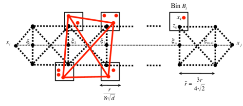
Figure 2: Construction of chain $G_{ij}$ for case $d=2$.

Proof(Theorem 6.1).

Consider a force flow $\gamma=\{G_{ij}\}_{1\leq i,j\leq n}$. Using lemma 6.2, we have

$$\sum_{i,j}\left|\langle x_{i}-x_{j},y_{i}-y_{j}\rangle\right| \leq Cr^{-1}\sum_{i,j}\sum_{(l,k)\in E(G_{ij})}\left|\langle x_{l}-x_{k},y_{l}-y_{k}\rangle\right|$$

$$\leq Cr^{-1}\sum_{(l,k)\in E(G)}\Big{(}\sum_{G_{ij}:(l,k)\in E(G_{ij})}1\Big{)}\left|\langle x_{l}-x_{k},y_{l}-y_{k}\rangle\right|$$

$$=Cr^{-1}\sum_{(l,k)\in E(G)}b(\gamma,(l,k))\left|\langle x_{l}-x_{k},y_{l}-y_{k}\rangle\right|,$$ (19)

where $b(\gamma,(l,k))$ denotes the number of chains passing through edge $(l,k)$. Notice that in Eq. (19), $b(\gamma,(l,k))$ is the only term that depends on the force flow $\gamma$. Hence, $b(\gamma,(l,k))$ can be replaced by its expectation under a probability distribution on $\Gamma$. According to Lemma 6.1, under the described distribution on $\Gamma$, the average number of chains containing any particular edge is upper bounded by $Cr^{-d-1}$, w.h.p. Therefore,

$$\sum_{i,j}\left|\langle x_{i}-x_{j},y_{i}-y_{j}\rangle\right|\leq Cr^{-d-2}\sum_{(l,k)\in E(G)}\left|\langle x_{l}-x_{k},y_{l}-y_{k}\rangle\right|.$$

Equivalently, $\|\mathcal{R}_{K_{n},X}(Y)\|_{1}\leq Cr^{-d-2}\|\mathcal{R}_{G,X}(Y)\|_{1}$, with high probability. ∎

6.1.1 Proof of Lemma 6.2

Proof.

Assume that $|V(G_{ij})|=m+1$ . Relabel the vertices in the chain $G_{ij}$ such that the nodes $i$ and $j$ have labels $0$ and $m$ respectively, and all the other nodes are labeled in $\{1,\cdots,m-1\}$. Since both sides of the desired inequality are invariant to translations, without loss of generality we assume that $x_{0}=y_{0}=0$. For a fixed vector $y_{m}$ consider the following optimization problem:

$$\Theta=\min_{y_{1},\cdots,y_{m-1}\in\mathbb{R}^{d}}\sum_{(l,k)\in E(G_{ij})}\left|\langle x_{l}-x_{k},y_{l}-y_{k}\rangle\right|.$$

To each edge $(l,k)\in E(G_{ij})$, assign a number $\lambda_{lk}$. (Note that $\lambda_{lk}=\lambda_{kl}$). For any assignment with $\max_{(l,k)\in E(G_{ij})}|\lambda_{lk}|\leq 1$, we have

$$\Theta \geq\min_{y_{1},\cdots,y_{m-1}\in\mathbb{R}^{d}}\sum_{(l,k)\in E(G_{ij})}\lambda_{lk}\langle x_{l}-x_{k},y_{l}-y_{k}\rangle$$

$$=\min_{y_{1},\cdots,y_{m-1}\in\mathbb{R}^{d}}\sum_{\begin{subarray}{c}l\in G_{ij}\\ l\neq 0\end{subarray}}\sum_{k\in\partial{l}}\lambda_{lk}\langle y_{l},x_{l}-x_{k}\rangle$$

$$=\min_{y_{1},\cdots,y_{m-1}\in\mathbb{R}^{d}}\sum_{\begin{subarray}{c}l\in G_{ij}\\ l\neq 0\end{subarray}}\langle y_{l},\sum_{k\in\partial{l}}\lambda_{lk}(x_{l}-x_{k})\rangle,$$

where $\partial{l}$ denotes the set of adjacent vertices to $l$ in $G_{ij}$. Therefore,

$$\Theta\geq\max_{\lambda_{lk}:|\lambda_{lk}|\leq 1}\;\min_{y_{1},\cdots,y_{m-1}\in\mathbb{R}^{d}}\sum_{\begin{subarray}{c}l\in G_{ij}\\ l\neq 0\end{subarray}}\langle y_{l},\sum_{k\in\partial{l}}\lambda_{lk}(x_{l}-x_{k})\rangle.$$ (20)

Note that the numbers $\lambda_{lk}$ that maximize the right hand side should satisfy $\sum_{k\in\partial{l}}\lambda_{lk}(x_{l}-x_{k})=0,\forall l\neq 0,m.$ Thus, $\Theta\geq\langle y_{m},\sum_{k\in\partial{m}}\lambda_{mk}(x_{m}-x_{k})\rangle$. Assume that we find values $\lambda_{lk}$ such that

$$\begin{split}\begin{cases}\sum_{k\in\partial{l}}\lambda_{lk}(x_{l}-x_{k})=0&\forall l\neq 0,m,\\ \sum_{k\in\partial{m}}\lambda_{mk}(x_{m}-x_{k})=x_{m},\\ \underset{(l,k)\in E(G_{ij})}{\max}|\lambda_{lk}|\leq Cr^{-1}.\end{cases}\end{split}$$ (21)

Given these values $\lambda_{lk}$, define $\tilde{\lambda}_{lk}=\dfrac{\lambda_{lk}}{\underset{(l,k)\in E(G_{ij})}{\max}|\lambda_{lk}|}$. Then $|\tilde{\lambda}_{lk}|\leq 1$ and

$$\Theta\geq\langle y_{m},\sum_{k\in\partial{m}}\tilde{\lambda}_{mk}(x_{m}-x_{k})\rangle=\langle y_{m},\frac{1}{\max_{l,k}|\lambda_{lk}|}x_{m}\rangle\geq Cr\langle y_{m},x_{m}\rangle,$$

which proves the thesis.

Notice that for any values $\lambda_{lk}$ satisfying (21), we have

$$\begin{cases}&\sum_{l\in V(G_{ij})}\sum_{k\in\partial{l}}\lambda_{lk}(x_{l}-x_{k})=\sum_{k\in\partial{0}}\lambda_{0k}(x_{0}-x_{k})+x_{m}\\ &\sum_{l\in V(G_{ij)}}\sum_{k\in\partial{l}}\lambda_{lk}(x_{l}-x_{k})=\sum_{(l,k)\in E(G_{ij})}\lambda_{lk}(x_{l}-x_{k})+\lambda_{kl}(x_{k}-x_{l})=0\end{cases}$$

Hence, $\sum_{k\in\partial{0}}\lambda_{0k}(x_{0}-x_{k})=-x_{m}$.

It is convenient to generalize the constraints in Eq. (21). Consider the following linear system of equations with unknown variables $\lambda_{lk}$.

$$\sum_{k\in\partial{l}}\lambda_{lk}(x_{l}-x_{k})=u_{l},\quad\text{for}\;l=0,\cdots,m.$$ (22)

Writing Eq. (22) in terms of the rigidity matrix of $G_{ij}$, and using the characterization of its null space as discussed in section 2.1, it follows that Eq. (22) have a solution if and only if

$$\sum_{i=0}^{m}u_{i}=0,\quad\sum_{i=0}^{m}u_{i}^{T}Ax_{i}=0,$$ (23)

where $A\in\mathbb{R}^{d\times d}$ is an arbitrary anti-symmetric matrix.

A mechanical interpretation. For any pair $(l,k)\in E(G_{ij})$, assume a spring with spring constant $\lambda_{lk}$ between nodes $l$ and $k$. Then, by Eq. (22), $u_{l}$ will be the force imposed on node $l$. The first constraint in Eq. (23) states that the net force on $G_{ij}$ is zero (force equilibrium), while the second condition states that the net torque is zero (torque equilibrium).

Indeed, $\sum_{i=0}^{m}u_{i}^{T}Au_{i}=\langle A,\sum_{i=0}^{m}u_{i}x_{i}^{T}\rangle=0$, for every anti-symmetric matrix $A$ if and only if $\sum_{i=0}^{m}u_{i}x_{i}^{T}$ is a symmetric matrix. Therefore,

$$\sum_{i=0}^{m}u_{i}\wedge x_{i}=\sum_{i=0}^{m}\left(\sum_{\ell=1}^{d}u_{i}^{(\ell)}e_{\ell}\right)\wedge\left(\sum_{k=1}^{d}x_{i}^{(k)}e_{k}\right)=\sum_{\ell,k}\sum_{i=0}^{m}(u_{i}^{(\ell)}x_{i}^{(k)}-x_{i}^{(\ell)}u_{i}^{(k)})(e_{\ell}\wedge e_{k})=0.$$

With this interpretation in mind, we propose a two-part procedure to find the spring constants $\lambda_{lk}$ that obey the constraints in (21).

Part (i): For the sake of simplicity, we focus here on the special case $d=2$. The general argument proceeds along the same lines and is deferred to Appendix K.

Consider the chain $G_{ij}$ between nodes $i$ and $j$, cf. Fig. 1. For every $1\leq p\leq k$, let $\mathcal{F}_{p}$ denote the common side of $H_{p}$ and $H_{p+1}$. Without loss of generality, assume $V(\mathcal{F}_{p})=\{1,2\}$, and $x_{m}$ is in the direction of $e_{1}$. Find the forces $f_{1}$, $f_{2}$ such that

$$\begin{split}f_{1}+f_{2}&=x_{m},\quad f_{1}\wedge x_{1}+f_{2}\wedge x_{2}=0,\\ &\|f_{1}\|^{2}+\|f_{2}\|^{2}\leq C\|x_{m}\|^{2}.\end{split}$$ (24)

To this end, we solve the following optimization problem.

$$\begin{split}&\text{minimize}\quad\;\frac{1}{2}(\|f_{1}\|^{2}+\|f_{2}\|^{2})\\ &\text{subject to}\quad f_{1}+f_{2}=x_{m},\quad f_{1}\wedge x_{1}+f_{2}\wedge x_{2}=0\end{split}$$ (25)

It is easy to see that the solutions of (LABEL:eq:opt) are given by

$$\begin{cases}f_{1}=\frac{1}{2}x_{m}+\frac{1}{2}\gamma A(x_{1}-x_{2})\\ f_{2}=\frac{1}{2}x_{m}-\frac{1}{2}\gamma A(x_{1}-x_{2})\end{cases}$$

$$\gamma=-\frac{1}{\|x_{1}-x_{2}\|^{2}}x_{m}^{T}A(x_{1}+x_{2}),\quad A=\begin{pmatrix}0&-1\\ 1&0\end{pmatrix}.$$

Now, we should show that the forces $f_{1}$ and $f_{2}$ satisfy the constraint $\|f_{1}\|^{2}+\|f_{2}\|^{2}\leq C\|x_{m}\|^{2}$, for some constant $C$. Clearly, it suffices to prove $\|\gamma(x_{1}-x_{2})\|\leq C\|x_{m}\|$. Observe that

$$\frac{\|\gamma(x_{1}-x_{2})\|}{\|x_{m}\|} =\frac{1}{\|x_{1}-x_{2}\|}\bigg{|}\frac{x_{m}^{T}}{\|x_{m}\|}A(x_{1}+x_{2})\bigg{|}$$

$$=\frac{1}{\|x_{1}-x_{2}\|}|e_{1}^{T}A(x_{1}+x_{2})|$$

$$=\frac{1}{\|x_{1}-x_{2}\|}|e_{2}^{T}(x_{1}+x_{2})|.$$

From the construction of chain $G_{ij}$, we have

$$|e_{2}^{T}(x_{1}+x_{2})|\leq\frac{r}{4},\quad\|x_{1}-x_{2}\|\geq\frac{r}{4},$$

which shows that $\|\gamma(x_{1}-x_{2})\|\leq\|x_{m}\|$.

Part (ii): For each $H_{p}$ consider the following set of forces

$$u_{i}=\begin{cases}f_{i}\;&\text{if}\;i\in V(\mathcal{F}_{p})\\ -f_{i}&\text{if}\;i\in V(\mathcal{F}_{p-1})\end{cases},\;$$ (26)

Also, let $u_{0}=-x_{m}$ and $u_{m}=x_{m}$. (cf. Fig. 3).

Notice that $\sum_{i\in V(H_{p})}u_{i}=0$, $\sum_{i\in V(H_{p})}u_{i}\wedge x_{i}=0$, and thus by the discussion prior to Eq. (23), there exist values $\lambda_{lk}^{(H_{p})}$, such that

$$\sum_{k:(l,k)\in E(H_{p})}\lambda_{lk}^{(H_{p})}(x_{l}-x_{k})=u_{l},\quad\forall l\in V(H_{p}).$$

Writing this in terms of $R^{(H_{p})}$, the rigidity matrix of $H_{p}$, we have

$$(R^{(H_{p})})^{T}\underline{\lambda}^{(H_{p})}=\underline{u},$$ (27)

where the vector $\underline{\lambda}^{(H_{p})}=[\lambda^{(H_{p})}_{lk}]$ has size $|E(H_{p})|=d(d+1)2^{d-2}$, and the vector $\underline{u}=[u_{l}]$ has size $d\times|V(H_{p})|=d2^{d}$. Among the solutions of Eq. (27), choose the one that is orthogonal to the nullspace of $(R^{(H_{p})})^{T}$. Therefore,

$$\sigma_{\min}(R^{(H_{p})})\|\lambda^{(H_{p})}\|_{\infty}\leq\sigma_{\min}(R^{(H_{p})})\|\lambda^{(H_{p})}\|_{2}\leq\|u\|\leq C\|x_{m}\|.$$

Form the construction of the chains, $H_{p}$ is a perturbation of the d-dimensional hypercube with side length $\tilde{r}=\frac{3r}{4\sqrt{2}}$. (each vertex wiggles by at most $\frac{r}{8}$). Using the fact that $\sigma_{\min}(.)$ is a Lipschitz continuos function of its argument, we get that $\sigma_{\min}(R^{(H_{p})})\geq Cr$, for some constant $C=C(d)$. Also, $\|x_{m}\|\leq 1$. Hence, $\|\lambda^{(H_{p})}\|_{\infty}\leq Cr^{-1}$.

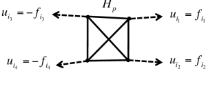
Figure 3: $H_{p}$ and the set of forces in Part $(ii)$

Now define

$$\lambda_{lk}=\sum_{H_{p}:(l,k)\in E(H_{p})}\lambda^{(H_{p})}_{lk},\quad\quad\forall(l,k)\in E(G_{ij}).$$ (28)

We claim that the values $\lambda_{lk}$ satisfy the constraints in (21).

First, note that for every node $l$,

$$\sum_{k\in\partial{l}}\lambda_{lk}(x_{l}-x_{k}) =\sum_{k\in\partial{l}}\left(\sum_{H_{p}:(l,k)\in E(H_{p})}\lambda_{lk}^{(H_{p})}\right)(x_{l}-x_{k})$$

$$=\sum_{H_{p}:l\in V(H_{p})}\left(\sum_{k:(l,k)\in E(H_{p})}\lambda_{lk}^{(H_{p})}(x_{l}-x_{k})\right)$$

$$=\sum_{H_{p}:l\in V(H_{p})}u_{l}.$$ (29)

For nodes $l\notin\{0,m\}$, there are two $H_{p}$ containing $l$. In one of them, $u_{l}=f_{l}$ and in the other $u_{l}=-f_{l}$. Hence, the forces $u_{l}$ cancel each other in Eq. (29) and the sum is zero. At nodes $0$ and $m$, this sum is equal to $-x_{m}$ and $x_{m}$ respectively.

Second, since each edge participates in at most two $H_{p}$, it follows from Eq. (28) that $|\lambda_{lk}|\leq Cr^{-1}$. ∎

7 Proof of Theorem 1.1 (Lower Bound)

Proof.

Consider the ‘bending’ map $\mathcal{T}:[-0.5,0.5]^{d}\to\mathbb{R}^{d+1}$, defined as

$$\mathcal{T}(t_{1},t_{2},\cdots,t_{d})=(R\sin\frac{t_{1}}{R},t_{2},\cdots,t_{d},R(1-\cos\frac{t_{1}}{R}))$$

This map bends the hypercube in the $d+1$ dimensional space. Here, $R$ is the curvature radius of the embedding (for instance, $R\gg 1$ corresponds to slightly bending the hypercube, cf. Fig. 4).

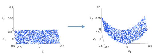
Figure 4: Bending map $\mathcal{T}$, with $R=2$, and $d=2$.

Now for a given $\Delta$, let $R=\max\{1,r^{2}\Delta^{-1/2}\}$ and give the distances $\tilde{d}_{ij}=\|\mathcal{T}(x_{i})-\mathcal{T}(x_{j})\|$ as the input distance measurements to the algorithm. First we show that these adversarial measurements satisfy the noise constraint $\|\tilde{d}^{2}_{ij}-d^{2}_{ij}\|\leq\Delta$.

$$d^{2}_{ij}-\tilde{d}^{2}_{ij} =(x_{i}^{(1)}-x_{j}^{(1)})^{2}-R^{2}\Big{[}\sin\Big{(}\frac{x_{i}^{(1)}}{R}\Big{)}-\sin\Big{(}\frac{x_{j}^{(1)}}{R}\Big{)}\Big{]}^{2}$$

$$-R^{2}\Big{[}\cos\Big{(}\frac{x_{i}^{(1)}}{R}\Big{)}-\cos\Big{(}\frac{x_{j}^{(1)}}{R}\Big{)}\Big{]}^{2}$$

$$=(x_{i}^{(1)}-x_{j}^{(1)})^{2}-R^{2}\Big{[}2-2\cos\Big{(}\frac{x_{i}^{(1)}-x_{j}^{(1)}}{R}\Big{)}\Big{]}$$

$$\leq\frac{(x_{i}^{(1)}-x_{j}^{(1)})^{4}}{2R^{2}}\leq\frac{r^{4}}{2R^{2}}\leq\Delta.$$

Also, $\tilde{d}_{ij}\leq d_{ij}$. Therefore, $|z_{ij}|=|\tilde{d}^{2}_{ij}-d^{2}_{ij}|\leq\Delta$.

The crucial point is that the SDP in the first step of the algorithm is oblivious of dimension $d$. Therefore, given the measurements $\tilde{d}_{ij}$ as the input, the SDP will return the Gram matrix $Q$ of the positions $\tilde{x}_{i}=L\mathcal{T}(x_{i})$, i.e., $Q_{ij}=\tilde{x}_{i}\cdot\tilde{x}_{j}$. Denote by $\{u_{1},\cdots,u_{d}\}$, the eigenvectors of $Q$ corresponding to the $d$ largest eigenvalues. Next, the algorithm projects the positions $\{\tilde{x}_{i}\}_{i\in[n]}$ onto the space $U=\langle u_{1},\cdots,u_{d}\rangle$ and returns them as the estimated positions in $\mathbb{R}^{d}$. Hence,

$$d(X,\widehat{X})=\frac{1}{n^{2}}\|XX^{T}-P_{U}\tilde{X}\tilde{X}^{T}P_{U}\|_{1}.$$

Let $W=\langle e_{1},e_{2},\cdots,e_{d}\rangle$ (see Fig. 5). Then,

$$d(X,\widehat{X})\geq\frac{1}{n^{2}}\|XX^{T}-\tilde{X}P_{W}\tilde{X}^{T}\|_{1}-\frac{1}{n^{2}}\|\tilde{X}P_{W}\tilde{X}^{T}-P_{U}\tilde{X}\tilde{X}^{T}P_{U}\|_{1}.$$ (30)

We bound each terms on the right hand side separately. For the first term,

$$\frac{1}{n^{2}}\|XX^{T}-\tilde{X}P_{W}\tilde{X}^{T}\|_{1}$$

$$=\frac{1}{n^{2}}\sum_{1\leq i,j\leq n}\bigg{|}x_{i}^{(1)}x_{j}^{(1)}-R^{2}\sin\Big{(}\frac{x_{i}^{(1)}}{R}\Big{)}\sin\Big{(}\frac{x_{j}^{(1)}}{R}\Big{)}\bigg{|}$$

$$\stackrel{{\scriptstyle(a)}}{{=}}\frac{1}{n^{2}}\sum_{1\leq i,j\leq n}\bigg{|}x_{i}^{(1)}x_{j}^{(1)}-R^{2}\Big{(}\frac{x_{i}^{(1)}}{R}-\frac{(x_{i}^{(1)})^{3}}{3!R^{3}}+\frac{\xi_{i}^{5}}{5!R^{5}}\Big{)}\Big{(}\frac{x_{j}^{(1)}}{R}-\frac{(x_{j}^{(1)})^{3}}{3!R^{3}}+\frac{\xi_{j}^{5}}{5!R^{5}}\Big{)}\bigg{|}$$

$$\stackrel{{\scriptstyle(b)}}{{\geq}}C\bigg{(}\frac{R}{n}\bigg{)}^{2}\sum_{1\leq i,j\leq n}\bigg{|}\frac{1}{3!}\Big{(}\frac{x_{i}^{(1)}}{R}\Big{)}\Big{(}\frac{x_{j}^{(1)}}{R}\Big{)}^{3}+\frac{1}{3!}\Big{(}\frac{x_{j}^{(1)}}{R}\Big{)}\Big{(}\frac{x_{i}^{(1)}}{R}\Big{)}^{3}\bigg{|}$$

$$\geq\frac{C}{(nR)^{2}}\Big{(}\sum_{1\leq i\leq n}|x_{i}^{(1)}|\Big{)}\Big{(}\sum_{1\leq j\leq n}|x_{i}^{(1)}|^{3}\Big{)}\geq\frac{C}{R^{2}},$$ (31)

where $(a)$ follows from Taylor’s theorem, and $(b)$ follows from $|\xi_{i}/R|\leq|x_{i}/R|\leq 1/2$.

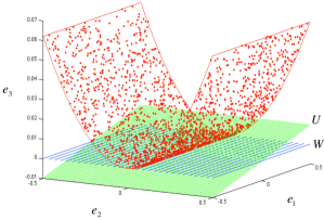
Figure 5: An illustration of subspaces $U$ and $W$.

The next Proposition provides an upper bound for the second term on the right hand side of Eq. (30).

Proposition 7.1.

The following is true.

$$\frac{1}{n^{2}}\|\tilde{X}P_{W}\tilde{X}^{T}-P_{U}\tilde{X}\tilde{X}^{T}P_{U}\|_{1}\to 0\text{ a.s.},\quad\text{as }n\to\infty.$$

Proof of this Proposition is provided in the next section.

Using the bounds given by Proposition 7.1 and Eq. (31), we obtain that, w.h.p.,

$$d(X,\widehat{X})\geq\frac{C_{1}}{R^{2}}\geq C\min\{1,\frac{\Delta}{r^{4}}\}.$$

The result follows. ∎

7.1 Proof of Proposition 7.1

We first establish the following remarks.

Remark 7.1.

Let $a,\;b\in{\mathbb{R}}^{m}$ be two unitary vectors. Then,

$$\|aa^{T}-bb^{T}\|_{2}=\sqrt{1-(a^{T}b)^{2}}.$$

For proof, we refer to Appendix L

Remark 7.2.

Assume $A$ and $\tilde{A}$ are $p\times p$ matrices. Let $\{\lambda_{i}\}$ be the eigenvalues of A such that $\lambda_{1}\geq\cdots\geq\lambda_{p-1}>\lambda_{p}$. Also, let $v$ and $\tilde{v}$ respectively denote the eigenvectors of $A$ and $\tilde{A}$ corresponding to their smallest eigenvalues. Then,

$$1-(v^{T}\tilde{v})^{2}\leq\frac{4\|A-\tilde{A}\|_{2}}{\lambda_{p-1}-\lambda_{p}}.$$

The proof is deferred to Appendix M.

Proof(Proposition 7.1).

Let $\tilde{X}=\sum_{i=1}^{d+1}\sigma_{i}u_{i}\hat{w}_{i}^{T}$ be the singular value decomposition of $\tilde{X}$, where $\|u_{i}\|=\|\hat{w}_{i}\|=1$, $u_{i}\in{\mathbb{R}}^{n}$, $\hat{w}_{i}\in{\mathbb{R}}^{d+1}$ and $\sigma_{1}\geq\sigma_{2}\geq\cdots\geq\sigma_{d+1}$. Notice that

$$P_{U}\tilde{X}=\sum_{i=1}^{d}\sigma_{i}u_{i}\hat{w}_{i}^{T}=(\sum_{i=1}^{d+1}\sigma_{i}u_{i}\hat{w}_{i}^{T})(\sum_{j=1}^{d}\hat{w}_{j}\hat{w}_{j}^{T})=\tilde{X}P_{\hat{W}},$$

where $\hat{W}=\langle\hat{w}_{1},\cdots,\hat{w}_{d}\rangle$, and $P_{\hat{W}}\in{\mathbb{R}}^{(d+1)\times(d+1)}$. Hence, $P_{U}\tilde{X}{\tilde{X}}^{T}P_{U}=\tilde{X}P_{\hat{W}}{\tilde{X}}^{T}$. Define $M=P_{\hat{W}}-P_{W}$. Then, we have

$$\frac{1}{n^{2}}\|\tilde{X}P_{W}\tilde{X}^{T}-P_{U}\tilde{X}\tilde{X}^{T}P_{U}\|_{1} =\frac{1}{n^{2}}\|\tilde{X}M\tilde{X}^{T}\|_{1}=\frac{1}{n^{2}}\sum_{1\leq i,j\leq n}|\tilde{x}_{i}^{T}M\tilde{x}_{j}|$$

$$\leq\frac{1}{n^{2}}\|M\|_{2}\sum_{1\leq i,j\leq n}\|\tilde{x}_{i}\|\|\tilde{x}_{j}\|\leq\|M\|_{2}.$$ (32)

Now, we need to bound $\|M\|_{2}$. We have,

$$M=P_{\hat{W}}-P_{W}=(I-P_{\hat{w}_{d+1}})-(I-P_{e_{d+1}})=P_{e_{d+1}}-P_{\hat{w}_{d+1}}.$$

Using Remark 7.1, we obtain $\|M\|_{2}=\|e_{d+1}e_{d+1}^{T}-\hat{w}_{d+1}\hat{w}_{d+1}^{T}\|_{2}=\sqrt{1-(e_{d+1}^{T}\hat{w}_{d+1})^{2}}$.

Let $Z_{i}=\tilde{x}_{i}\tilde{x}_{i}^{T}\in{\mathbb{R}}^{(d+1)\times(d+1)}$, $\bar{Z}=\frac{1}{n}\sum_{i=1}^{n}Z_{i}$ and $Z=\mathbb{E}(Z_{i})$. Notice that $\bar{Z}=\frac{1}{n}\tilde{X}^{T}\tilde{X}=\frac{1}{n}\sum_{i=1}^{d+1}\sigma_{i}^{2}\hat{w}_{i}\hat{w}_{i}^{T}$. Therefore, $\hat{w}_{d+1}$ is the eigenvector of $\bar{Z}$ corresponding to its smallest eigenvalue. In addition, $Z$ is a diagonal matrix (with $Z_{(d+1),(d+1)}$ the smallest diagonal entry). Hence, $e_{d+1}$ is its eigenvector corresponding to the smallest eigenvalue, $Z_{(d+1),(d+1)}$.

By applying Remark 7.2, we have

$$\|M\|_{2}\leq\sqrt{1-(e_{d+1}^{T}\hat{w}_{d+1})^{2}}\leq\sqrt{\frac{4\|Z-\bar{Z}\|_{2}}{\lambda_{d}-\lambda_{d+1}}},$$ (33)

where $\lambda_{d}>\lambda_{d+1}$ are the two smallest eigenvalues of $Z$. Let $t$ be a random variable, uniformly distributed in $[-0.5,0.5]$. Then,

$$\lambda_{d}=\mathbb{E}\bigg{[}R^{2}\sin^{2}\bigg{(}\frac{t}{R}\bigg{)}\bigg{]}\quad\text{and}\quad\lambda_{d+1}=\mathbb{E}\bigg{[}R^{2}\bigg{(}1-\cos^{2}\bigg{(}\frac{t}{R}\bigg{)}\bigg{)}\bigg{]}.$$

Hence, $\lambda_{d}-\lambda_{d+1}=R^{3}(-1/R-\sin(1/R)+4\sin(1/2R))\geq 0.07$, since $R\geq 1$.

Also, note that $\{Z_{i}\}_{1\leq i\leq n}$ is a sequence of iid random matrices with dimension $(d+1)$ and $\|Z\|_{\infty}=\|\mathbb{E}(Z_{i})\|_{\infty}<\infty$. By Law of large numbers, $\bar{Z}\to Z$, almost surely. Now, since the operator norm is a continuos function, we have $\|Z-\bar{Z}\|_{2}\to 0$, almost surely. The result follows directly from Eqs. (32) and (33).

∎

8 Numerical experiments

Theorem 1.1 considers a worst case model for the measurement noise in which the errors $\{z_{ij}\}_{(i,j)\in E}$ are arbitrary but uniformly bounded as $|z_{ij}|\leq\Delta$. The proof of the lower bound (cf. Section 7) introduces errors $\{z_{ij}\}_{(i,j)\in E}$ defined based on a bending map, $\mathcal{T}$. This set of errors results in the claimed lower bound. For clarity, we denote this set of errors by $\{z^{\mathcal{T}}_{ij}\}$. In this section, we consider a mixture model for the measurement errors. For given parameters $\Delta$ and ${\varepsilon}$, we let

$$z_{ij}\sim{\varepsilon}\gamma_{\Delta/2}+(1-{\varepsilon})\delta_{z^{\mathcal{T}}_{i,j}},$$ (34)

where $\gamma_{\sigma}(x)=1/(\sqrt{2\pi}\sigma)e^{-x^{2}/2\sigma^{2}}$ is the density function of the normal distribution with mean zero and variance $\sigma^{2}$. The goal of the numerical experiments is to show the dependency of the algorithm performance on each of the parameters $n,r$ and $\Delta$. We consider the following configurations. For each configuration we run the SDP-based algorithm and evaluate $d(X,\widehat{X})$. The error bars in figures correspond to $10$ realizations of that configuration. Throughout the measurement errors are defined according to (34) with ${\varepsilon}=0.1$.

1. Fix $\Delta=0.005$ and $d\in\{2,4\}$. Let $r=3(\log n/n)^{1/d}$, with $n\in\{100,120,140,\cdots,300\}$. Fig. 6 summarizes the results. According to the plot, $d(X,\widehat{X})\propto n^{2}$ for $d=2$ and $d(X,\widehat{X})\propto n$ for $d=4$.

2. Fix $\Delta=0.005$, $d=2$ and $n=150$. Let $r\in\{0.5,0.55,0.6,\cdots,0.8\}$. The results are shown in Fig. 7. As we see, $d(X,\widehat{X})$ is fairly proportional to $r^{-4}$.

3. Fix $n=150$, $r=0.6$ and $d=2$. Let $\Delta\in\{0.005,0.01,0.015,0.02,0.025\}$. Fig. 8 showcases the results. The performance deteriorates linearly with respect to $\Delta$.

Acknowledgment. Adel Javanmard is supported by Caroline and Fabian Pease Stanford Graduate Fellowship. This work was partially supported by the NSF CAREER award CCF-0743978, the NSF grant DMS-0806211, and the AFOSR grant FA9550-10-1-0360. The authors thank the anonymous reviewers for their insightful comments.

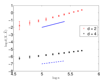
Figure 6: Performance results for $\Delta=0.005$, $d=2,4$, and $r=3(\log n/n)^{1/d}$. The plot shows $\log\,d(X,\widehat{X})$ vs. $\log n$ for a set of values of $n$. The solid line and the dashed line respectively correspond to $d(X,\widehat{X})\propto n^{2}$ and $d(X,\widehat{X})\propto n$ and are plotted as reference.

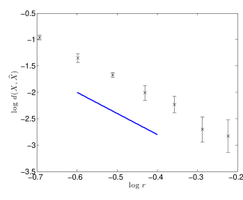
Figure 7: Performance results for $\Delta=0.005$, $d=2$, and $n=150$. The plot shows $\log\,d(X,\widehat{X})$ vs. $\log r$ for a set of values of $r$. The solid line corresponds to $d(X,\widehat{X})\propto r^{-4}$ and is plotted as reference.

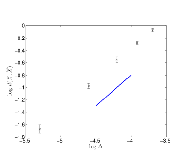
Figure 8: Performance results for $n=150$, $r=0.6$, and $d=2$. The plot shows $\log\,d(X,\widehat{X})$ vs. $\log\Delta$ for a set of values of $\Delta$. The solid line corresponds to $d(X,\widehat{X})\propto\Delta$ and is plotted as reference.

Appendix A Proof of Remark 2.1

For $1\leq j\leq n$, let random variable $z_{j}$ be $1$ if node $j$ is in region $\mathcal{R}$ and 0 otherwise. The variables $\{z_{j}\}$ are i.i.d. Bernoulli with probability $V(\mathcal{R})$ of success. Also, $n(\mathcal{R})=\sum_{j=1}^{n}z_{j}$.

By application of the Chernoff bound we obtain

$$\mathbb{P}\Big{(}\Big{|}\sum_{j=1}^{n}z_{j}-nV(\mathcal{R})\Big{|}\geq\delta nV(\mathcal{R})\Big{)}\geq 2\exp\Big{(}-\frac{\delta^{2}nV(\mathcal{R})}{2}\Big{)}.$$

Choosing $\delta=\sqrt{\dfrac{2c\log n}{nV(\mathcal{R})}}$, the right hand side becomes $2\exp(-c\log n)=2/n^{c}$. Therefore, with probability at least $1-2/n^{c}$,

$$n(\mathcal{R})\in nV(\mathcal{R})+[-\sqrt{2cnV(\mathcal{R})\log n},\sqrt{2cnV(\mathcal{R})\log n}].$$ (35)

Appendix B Proof of Proposition 5.1

We apply the bin-covering technique. Cover the space $[-0.5,0.5]^{d}$ with a set of non-overlapping hypercubes (bins) whose side lengths are $\delta$. Thus, there are a total of $m=\lceil{1/\delta}\rceil^{d}$ bins, each of volume $\delta^{d}$. In formula, bin $(j_{1},\cdots,j_{d})$ is the hypercube $[(j_{1}-1)\delta,j_{1}\delta)\times\cdots\times[(j_{d}-1)\delta,j_{d}\delta)$, for $j_{k}\in\{1,\cdots,\lceil 1/\delta\rceil\}$ and $k\in\{1,\cdots,d\}$. Denote the set of bins by $\{B_{k}\}_{1\leq k\leq m}$. Assume $n$ nodes are deployed uniformly at random in $[-0.5,0.5]^{d}$. We claim that if $\delta\geq(c\log n/n)^{1/d}$, where $c>1$, then w.h.p., every bin contains at least $d+1$ nodes.

Fix $k$ and let random variable $\xi_{l}$ be $1$ if node $l$ is in bin $B_{k}$ and $0$ otherwise. The variables $\{\xi_{l}\}_{1\leq l\leq n}$ are i.i.d. Bernoulli with probability $1/m$ of success. Also $\xi=\sum_{l=1}^{n}\xi_{l}$ is the number of nodes in bin $B_{k}$. By Markov inequality, $\mathbb{P}(\xi\leq d)\leq\mathbb{E}\{Z^{\xi-d}\}$, for any $0\leq Z\leq 1$. Choosing $Z=md/n$, we have

$$\mathbb{P}(\xi\leq d) \leq\mathbb{E}\{Z^{\xi-d}\}=Z^{-d}\prod_{l=1}^{n}\mathbb{E}\{Z^{\xi_{l}}\}$$

$$=Z^{-d}\left(\frac{1}{m}Z+1-\frac{1}{m}\right)^{n}=\left(\frac{n}{md}\right)^{d}\left(1+\frac{d}{n}-\frac{1}{m}\right)^{n}$$

$$\leq\left(\frac{ne}{md}\right)^{d}e^{-n/m}=\left(\frac{ne\delta^{d}}{d}\right)^{d}e^{-n\delta^{d}}\leq\Big{(}\frac{ce\log n}{d}\Big{)}^{d}n^{-c}.$$

By applying union bound over all the $m$ bins, we get the desired result.

Now take $\delta=r/(4\sqrt{d})$. Given that $r\geq 4c\sqrt{d}(\log n/n)^{1/d}$, for some $c>1$, every bin contains at least $d+1$ nodes, with high probability. Note that for any two nodes $x_{i},x_{j}\in[-0.5,0.5]^{d}$ with $\|x_{i}-x_{j}\|\leq r/2$, the point $(x_{i}+x_{j})/2$ (the midpoint of the line segment between $x_{i}$ and $x_{j}$) is contained in one of the bins, say $B_{k}$. For any point $s$ in this bin,

$$\|s-x_{i}\|\leq\Big{\|}s-\frac{x_{i}+x_{j}}{2}\Big{\|}+\Big{\|}\frac{x_{i}+x_{j}}{2}-x_{i}\Big{\|}\leq\frac{r}{4}+\frac{r}{4}=\frac{r}{2}.$$

Similarly, $\|s-x_{j}\|\leq r/2$. Since $s\in B_{k}$ was arbitrary, $\mathcal{C}_{i}\cap\mathcal{C}_{j}$ contains all the nodes in $B_{k}$. This implies the thesis, since $B_{k}$ contains at least $d+1$ nodes.

Appendix C Proof of Proposition 5.2

Let $m_{k}=|\mathcal{Q}_{k}|$ and define the matrix $R_{k}$ as follows.

$$R_{k}=\begin{bmatrix}x_{\mathcal{Q}_{k}}^{(1)}\Big{|}\cdots|x_{\mathcal{Q}_{k}}^{(d)}\Big{|}u_{\mathcal{Q}_{k}}\end{bmatrix}^{T}\in{\mathbb{R}}^{(d+1)\times m_{k}}.$$

Compute an orthonormal basis $w_{k,1},\cdots,w_{k,m_{k}-d-1}\in{\mathbb{R}}^{m_{k}}$ for the nullspace of $R_{k}$. Then

$$\Omega_{k}=P^{\perp}_{\langle u_{\mathcal{Q}_{k}},x^{(1)}_{\mathcal{Q}_{k}},\cdots,x^{(d)}_{\mathcal{Q}_{k}}\rangle}=\sum_{l=1}^{m_{k}-d-1}w_{k,l}w_{k,l}^{T}.$$

Let $\hat{w}_{k,l}\in{\mathbb{R}}^{n}$ be the vector obtained from $w_{k,l}$ by padding it with zeros. Then, $\hat{\Omega}_{k}=\sum_{l=1}^{m_{k}-d-1}\hat{w}_{k,l}\hat{w}_{k,l}^{T}$. In addition, the $(i,j)$ entry of $\hat{\Omega}_{k}$ is nonzero only if $i,j\in\mathcal{Q}_{k}$. Any two nodes in $\mathcal{Q}_{k}$ are connected in $G$ (Recall that $\mathcal{Q}_{k}$ is a cliques of $G$). Hence, $\hat{\Omega}_{k}$ is zero outside $E$. Since $\Omega=\sum_{\mathcal{Q}_{k}\in{\sf cliq}(G)}\hat{\Omega}_{k}$, the matrix $\Omega$ is also zero outside $E$.

Notice that for any $v\in\langle x^{(1)},\cdots,x^{(d)},u\rangle$,

$$\Omega v=(\sum_{\mathcal{Q}_{k}\in{\sf cliq}(G)}\hat{\Omega}_{k})v=\sum_{\mathcal{Q}_{k}\in{\sf cliq}(G)}\Omega_{k}v_{\mathcal{Q}_{k}}=0.$$

So far we have proved that $\Omega$ is a stress matrix for the framework. Clearly, $\Omega\succeq 0$, since $\hat{\Omega}_{k}\succeq 0$ for all $k$. We only need to show that ${\rm rank}(\Omega)=n-d-1$. Since $\text{Ker}(\Omega)\supseteq\langle x^{(1)},\cdots,x^{(d)},u\rangle$, we have $\text{rank}(\Omega)\leq n-d-1$. Define

$$\tilde{\Omega}=\sum_{\mathcal{Q}_{k}\in\{\mathcal{C}_{1},\cdots,\mathcal{C}_{n}\}}\hat{\Omega}_{k}.$$

Since $\Omega\succeq\tilde{\Omega}\succeq 0$, it suffices to show that ${\rm rank}(\tilde{\Omega})\geq n-d-1$. For an arbitrary vector $v\in\text{Ker}(\tilde{\Omega})$,

$$v^{T}\tilde{\Omega}v=\sum_{i=1}^{n}\|P^{\perp}_{\langle u_{\mathcal{C}_{i}},x^{(1)}_{\mathcal{C}_{i}},\cdots,x^{(d)}_{\mathcal{C}_{i}}\rangle}v_{\mathcal{C}_{i}}\|^{2}=0,$$

which implies that $v_{\mathcal{C}_{i}}\in\langle u_{\mathcal{C}_{i}},x^{(1)}_{\mathcal{C}_{i}},\cdots,x^{(d)}_{\mathcal{C}_{i}}\rangle$. Hence, the vector $v_{\mathcal{C}_{i}}$ can be written as

$$v_{\mathcal{C}_{i}}=\sum_{\ell=1}^{d}\beta^{(\ell)}_{i}x^{(\ell)}_{\mathcal{C}_{i}}+\beta^{(d+1)}_{i}u_{\mathcal{C}_{i}}$$

for some scalars $\beta^{(\ell)}_{i}$. Note that for any two nodes $i$ and $j$, the vector $v_{\mathcal{C}_{i}\cap\mathcal{C}_{j}}$ has the following two representations

$$v_{\mathcal{C}_{i}\cap\mathcal{C}_{j}}=\sum_{\ell=1}^{d}\beta^{(\ell)}_{i}x^{(\ell)}_{\mathcal{C}_{i}\cap\mathcal{C}_{j}}+\beta^{(d+1)}_{i}u_{\mathcal{C}_{i}\cap\mathcal{C}_{j}}=\sum_{\ell=1}^{d}\beta^{(\ell)}_{j}x^{(\ell)}_{\mathcal{C}_{i}\cap\mathcal{C}_{j}}+\beta^{(d+1)}_{j}u_{\mathcal{C}_{i}\cap\mathcal{C}_{j}}$$

Therefore,

$$\sum_{\ell=1}^{d}(\beta^{(\ell)}_{i}-\beta^{(\ell)}_{j})x^{(\ell)}_{\mathcal{C}_{i}\cap\mathcal{C}_{j}}+(\beta^{(d+1)}_{i}-\beta^{(d+1)}_{j})u_{\mathcal{C}_{i}\cap\mathcal{C}_{j}}=0$$ (36)

According to Proposition 5.1, with high probability, for any two nodes $i$ and $j$ with $\|x_{i}-x_{j}\|\leq r/2$, we have $|\mathcal{C}_{i}\cap\mathcal{C}_{j}|\geq d+1$. Thus, the vectors $x^{(\ell)}_{\mathcal{C}_{i}\cap\mathcal{C}_{j}}$, $u_{\mathcal{C}_{i}\cap\mathcal{C}_{j}}$, $1\leq\ell\leq d$ are linearly independent, since the configuration is generic. More specifically, let $Y$ be the matrix with $d+1$ columns $\{x^{(\ell)}_{\mathcal{C}_{i}\cap\mathcal{C}_{j}}\}_{\ell=1}^{d}$, $u_{\mathcal{C}_{i}\cap\mathcal{C}_{j}}$. Then, ${\rm det}(Y^{T}Y)$ is a nonzero polynomial in the coordinates $x^{(\ell)}_{k}$, $k\in\mathcal{C}_{i}\cap\mathcal{C}_{j}$ with integer coefficients. Since the configuration of the points is generic, ${\rm det}(Y^{T}Y)\neq 0$ yielding the linear independence of the columns of $Y$. Consequently, Eq. (36) implies that $\beta^{(\ell)}_{i}=\beta^{(\ell)}_{j}$ for any two adjacent nodes in $G(n,r/2)$. Given that $r>10\sqrt{d}(\log n/n)^{1/d}$, the graph $G(n,r/2)$ is connected w.h.p. and thus the coefficients $\beta^{(\ell)}_{i}$ are the same for all $i$. Dropping subscript $(i)$, we obtain

$$v=\sum_{\ell=1}^{d}\beta^{(\ell)}x^{(\ell)}+\beta^{(d+1)}u,$$

proving that $\text{Ker}(\tilde{\Omega})\subseteq\langle u,x^{(1)},\cdots,x^{(d)}\rangle$, and thus $\text{rank}(\tilde{\Omega})\geq n-d-1$.

Appendix D Proof of Claim 5.2

Let $\tilde{G}=(V,\tilde{E})$, where $\tilde{E}=\{(i,j):d_{ij}\leq r/2\}$. The Laplacian of $\tilde{G}$ is denoted by $\tilde{\mathcal{L}}$. We first show that for some constant $C$,

$$\tilde{\mathcal{L}}\preceq C\sum_{k=1}^{n}P_{u_{\mathcal{C}_{k}}}^{\perp}.$$ (37)

Note that,

$$\sum_{k=1}^{n}P_{u_{\mathcal{C}_{k}}}^{\perp} =\sum_{k=1}^{n}(I-\frac{1}{|\mathcal{C}_{k}|}u_{\mathcal{C}_{k}}u_{\mathcal{C}_{k}}^{T})=\sum_{k=1}^{n}\frac{1}{|\mathcal{C}_{k}|}\Big{(}\sum_{i,j\in\mathcal{C}_{k}}M_{ij}\Big{)}$$

$$\succeq\sum_{(i,j)\in\tilde{E}}\Big{(}\sum_{k:(i,j)\in\mathcal{C}_{k}}\frac{1}{|\mathcal{C}_{k}|}\Big{)}M_{ij}=\sum_{(i,j)\in\tilde{E}}\Big{(}\sum_{k\in\mathcal{C}_{i}\cap\mathcal{C}_{j}}\frac{1}{|\mathcal{C}_{k}|}\Big{)}M_{ij}.$$

The inequality follows from the fact that $M_{ij}\succeq\bf{0}$, $\forall i,j$. By application of Remark 2.1, we have $|\mathcal{C}_{k}|\leq C_{1}(nr^{d})$ and $|\mathcal{C}_{i}\cap\mathcal{C}_{j}|\geq C_{2}nr^{d}$, for some constants $C_{1}$ and $C_{2}$ (depending on $d$) and $\forall k,i,j$. Therefore,

$$\sum_{k=1}^{n}P_{u_{\mathcal{C}_{k}}}^{\perp}\succeq\sum_{(i,j)\in\tilde{E}}\frac{C_{2}}{C_{1}}M_{ij}=\frac{C_{2}}{C_{1}}\tilde{\mathcal{L}}.$$

Next we prove that for some constant $C$,

$$\mathcal{L}\preceq C\tilde{\mathcal{L}}.$$ (38)

To this end, we use the Markov chain comparison technique.

A path between two nodes $i$ and $j$, denoted by $\gamma_{ij}$, is a sequence of nodes $(i,v_{1},\cdots,v_{t-1},j)$, such that the consecutive pairs are connected in $\tilde{G}$. Let $\gamma=(\gamma_{ij})_{(i,j)\in E}$ denote a collection of paths for all pairs connected in $G$, and let $\Gamma$ be the collection of all possible $\gamma$. Consider the probability distribution induced on $\Gamma$ by choosing paths between all connected pairs in $G$ in the following way.

Cover the space $[-0.5,0.5]^{d}$ with bins of side length $r/(4\sqrt{d})$ (similar to the proof of Proposition 5.1. As discussed there, w.h.p., every bin contains at least one node). Paths are selected independently for different node pairs. Consider a particular pair $(i,j)$ connected in $G$. Select $\gamma_{ij}$ as follows. If $i$ and $j$ are in the same bin or in the neighboring bins then $\gamma_{ij}=(i,j)$. Otherwise, consider all bins intersecting the line joining $i$ and $j$. From each of these bins, choose a node $v_{k}$ uniformly at random. Then the path $\gamma_{ij}$ is $(i,v_{1},\cdots,j)$.

In the following, we compute the average number of paths passing through each edge in $\tilde{E}$. The total number of paths is $|E|=\Theta(n^{2}r^{d})$. Also, since any connected pair in $G$ are within distance $r$ of each other and the side length of the bins is $O(r)$, there are $O(1)$ bins intersecting a straight line joining a pair $(i,j)\in E$. Consequently, each path contains $O(1)$ edges. The total number of bins is $\Theta(r^{-d})$. Hence, by symmetry, the number of paths passing through each bin is $\Theta(n^{2}r^{2d})$. Consider a particular bin $B$ and the paths passing through it. All these paths are equally likely to choose any of the nodes in $B$. Therefore, the average number of paths containing a particular node in $B$, say $i$, is $\Theta(n^{2}r^{2d}/nr^{d})=\Theta(nr^{d})$. In addition, the average number of edges between $i$ and neighboring bins is $\Theta(nr^{d})$. Due to symmetry, the average number of paths containing an edge incident on $i$ is $\Theta(1)$. Since this is true for all nodes $i$, the average number of paths containing an edge is $\Theta(1)$.

Now, let $v\in{\mathbb{R}}^{n}$ be an arbitrary vector. For a directed edge $e\in\tilde{E}$ from $i\to j$, define $v(e)=v_{i}-v_{j}$. Also, let $|\gamma_{ij}|$ denote the length of the path $\gamma_{ij}$.

$$v^{T}\mathcal{L}v =\sum_{(i,j)\in E}(v_{i}-v_{j})^{2}=\sum_{(i,j)\in E}\bigg{(}\sum_{e\in\gamma_{ij}}v(e)\bigg{)}^{2}$$

$$\leq\sum_{(i,j)\in E}|\gamma_{ij}|\sum_{e\in\gamma_{ij}}v(e)^{2}=\sum_{e\in\tilde{E}}v(e)^{2}\sum_{\gamma_{ij}\ni e}|\gamma_{ij}|$$

$$\leq\gamma_{*}\sum_{e\in\tilde{E}}v(e)^{2}b(\gamma,e),$$ (39)

where $\gamma_{*}$ is the maximum path lengths and $b(\gamma,e)$ denotes the number of paths passing through $e$ under $\gamma=(\gamma_{ij})$. The first inequality follows from the Cauchy-Schwartz inequality. Since all paths have length $O(1)$, we have $\gamma_{*}=O(1)$. Also, note that in Eq. (39), $b(\gamma,e)$ is the only term that depends on the paths. Therefore, we can replace $b(\gamma,e)$ with its expectation under the distribution on $\Gamma$, i.e., $b(e)=\sum_{\gamma\in\Gamma}\mathbb{P}(\gamma)b(\gamma,e)$. We proved above that the average number of paths passing through an edge is $\Theta(1)$. Hence, $\underset{e\in\tilde{E}}{\max}\;b(\gamma,e)=\Theta(1)$. using these bounds in Eq. (39), we obtain

$$v^{T}\mathcal{L}v\leq C\sum_{e\in\tilde{E}}v(e)^{2}=Cv^{T}\tilde{\mathcal{L}}v,$$ (40)

for some constant $C$ and all vectors $v\in{\mathbb{R}}^{n}$. Combining Eqs. (37) and (40) implies the thesis.

Appendix E Proof of Claim 5.3

In Remark 2.1, let region $\mathcal{R}$ be the $r/2$-neighborhood of node $i$, and take $c=2$. Then, with probability at least $1-2/n^{2}$,

$$|\mathcal{C}_{i}|\in np_{d}+[-\sqrt{4np_{d}\log n},\sqrt{4np_{d}\log n}],$$ (41)

where $p_{d}=K_{d}(r/2)^{d}$. Similarly, with probability at least $1-2/n^{2}$,

$$|\tilde{\mathcal{C}_{i}}|\in n\tilde{p}_{d}+[-\sqrt{4n\tilde{p}_{d}\log n},\sqrt{4n\tilde{p}_{d}\log n}],$$ (42)

where $\tilde{p}_{d}=K_{d}(\frac{r}{2})^{d}(\frac{1}{2}+\frac{1}{100})^{d}$. By applying union bound over all $1\leq i\leq n$, Eqs. (41) and (42) hold for any $i$, with probability at least $1-4/n$. Given that $r>10\sqrt{d}(\log n/n)^{\frac{1}{d}}$, the result follows after some algebraic manipulations.

Appendix F Proof of Claim 5.4

Part $(i)$: Let $\tilde{G}=(V,\tilde{E})$, where $\tilde{E}=\{(i,j):d_{ij}\leq r/2\}$. Also, let $A_{\tilde{G}}$ and $A_{G^{*}}$ respectively denote the adjacency matrices of the graphs $\tilde{G}$ and $G^{*}$. Therefore, $A_{\tilde{G}}\in{\mathbb{R}}^{n\times n}$ and $A_{G^{*}}\in{\mathbb{R}}^{N\times N}$, where $N=|V(G^{*})|=n(m+1)$. From the definition of $G^{*}$, we have

$$A_{G^{*}}=A_{\tilde{G}}\otimes B,\quad B=\begin{bmatrix}1&\cdots&1\\ \vdots&\cdots&\vdots\\ 1&\cdots&1\end{bmatrix}_{(m+1)\times(m+1)}$$ (43)

where $\otimes$ stands for the Kronecher product. Hence,

$$\max_{i\in V(G^{*})}\text{deg}_{G^{*}}(i)=(m+1)\max_{i\in V(\tilde{G})}\text{deg}_{\tilde{G}}(i).$$

Since the degree of nodes in $\tilde{G}$ are bounded by $C(nr^{d})$ for some constant $C$, and $m\leq C(nr^{d})$ (by definition of $m$ in Claim 5.3), we have that the degree of nodes in $G^{*}$ are bounded by $C(nr^{d})^{2}$, for some constant $C$.

Part $(ii)$: Let $D_{\tilde{G}}\in{\mathbb{R}}^{n\times n}$ be the diagonal matrix with degrees of the nodes in $\tilde{G}$ on its diagonal. Define $D_{G^{*}}\in{\mathbb{R}}^{N\times N}$ analogously. From Eq. (43), it is easy to see that

$$(D_{\tilde{G}}^{-1/2}A_{\tilde{G}}D_{\tilde{G}}^{-1/2})\otimes(\frac{1}{m+1}B)=D^{-1/2}_{G^{*}}A_{G^{*}}D^{-1/2}_{G^{*}}.$$

Now for any two matrices $\mathcal{A}$ and $\mathcal{B}$, the eigenvalues of $\mathcal{A}\otimes\mathcal{B}$ are all products of eigenvalues of $\mathcal{A}$ and $\mathcal{B}$. The matrix $1/(m+1)B$ has eigenvalues $0$, with multiplicity $m$, and $1$, with multiplicity one. Thereby,

$$\sigma_{\min}(I-D^{-1/2}_{G^{*}}A_{G^{*}}D^{-1/2}_{G^{*}})\geq\min\{\sigma_{\min}(I-D_{\tilde{G}}^{-1/2}A_{\tilde{G}}D_{\tilde{G}}^{-1/2}),1\}\geq Cr^{2},$$

where the last step follows from Remark 2.2. Due to the result of [8] (Theorem 4), we obtain

$$\sigma_{\min}(\mathcal{L}_{G^{*}})\geq d_{\min,G^{*}}\sigma_{\min}(\mathcal{L}_{n,G^{*}}),$$

where $d_{\min,G^{*}}$ denotes the minimum degree of the nodes in $G^{*}$, and $\mathcal{L}_{n,G^{*}}=I-D^{-1/2}_{G^{*}}A_{G^{*}}D^{-1/2}_{G^{*}}$ is the normalized Laplacian of $G^{*}$. Since $d_{\min,G^{*}}=(m+1)d_{\min,\tilde{G}}\geq C(nr^{d})^{2}$, for some constant $C$, we obtain

$$\sigma_{\min}(\mathcal{L}_{G^{*}})\geq C(nr^{d})^{2}r^{2},$$

for some constant $C$.

Appendix G Proof of Claim 5.5

Fix a pair $(i,j)\in E(G^{*})$. Let $m_{ij}=|\mathcal{Q}_{i}\cap\mathcal{Q}_{j}|$, and without loss of generality assume that the nodes in $\mathcal{Q}_{i}\cap\mathcal{Q}_{j}$ are labeled with $\{1,\cdots,m_{ij}\}$. Let $z^{(\ell)}=\tilde{x}^{(\ell)}_{\mathcal{Q}_{i}\cap\mathcal{Q}_{j}}$, for $1\leq\ell\leq d$, and let $z_{k}=(z_{k}^{(1)},\cdots,z_{k}^{(d)})$, for $1\leq k\leq m_{ij}$. Define the matrix $M^{(ij)}\in{\mathbb{R}}^{d\times d}$ as $M^{(ij)}_{\ell,\ell^{\prime}}=\langle z^{(\ell)},z^{(\ell^{\prime})}\rangle$, for $1\leq\ell^{\prime},\ell\leq d$. Finally, let $\beta_{ij}=(\beta^{(1)}_{j}-\beta^{(1)}_{i},\cdots,\beta^{(d)}_{j}-\beta^{(d)}_{i})\in{\mathbb{R}}^{d}$. Then,

$$\|\sum_{\ell=1}^{d}(\beta^{(\ell)}_{j}-\beta^{(\ell)}_{i})\tilde{x}^{(\ell)}_{\mathcal{Q}_{i}\cap\mathcal{Q}_{j}}\|^{2}=\beta_{ij}^{T}M^{(ij)}\beta_{ij}\geq\sigma_{\min}(M^{(ij)})\|\beta_{ij}\|^{2}.$$ (44)

In the following, we lower bound $\sigma_{\min}(M^{(i,j)})$. Notice that

$$M^{(ij)}=\sum_{k=1}^{m_{ij}}z_{k}z_{k}^{T}=\sum_{k=1}^{m_{ij}}\{z_{k}z_{k}^{T}-\mathbb{E}(z_{k}z_{k}^{T})\}+\sum_{k=1}^{m_{ij}}\mathbb{E}(z_{k}z_{k}^{T}).$$ (45)

We first lower bound the quantity $\sigma_{\min}(\sum_{k=1}^{m_{ij}}\mathbb{E}(z_{k}z_{k}^{T}))$. Let $S\in{\mathbb{R}}^{d\times d}$ be an orthogonal matrix that aligns the line segment between $x_{i}$ and $x_{j}$ with $e_{1}$. Now, let $\hat{z_{k}}=Sz_{k}$ for $1\leq k\leq m_{ij}$. Then,

$$\sum_{k=1}^{m_{ij}}\mathbb{E}(z_{k}z_{k}^{T})=\sum_{k=1}^{m_{ij}}S^{T}\mathbb{E}(\hat{z}_{k}\hat{z}_{k}^{T})S.$$

The matrix $\mathbb{E}(\hat{z}_{k}\hat{z}_{k}^{T})$ is the same for all $1\leq k\leq m_{ij}$. Further, it is a diagonal matrix whose diagonal entries are bounded from below by $C_{1}r^{2}$, for some constant $C_{1}$. Therefore, $\sigma_{\min}(\sum_{k=1}^{m_{ij}}\mathbb{E}(\hat{z}_{k}\hat{z}_{k}^{T}))\geq m_{ij}C_{1}r^{2}$. Consequently,

$$\sigma_{\min}(\sum_{k=1}^{m_{ij}}\mathbb{E}(z_{k}z_{k}^{T}))=\sigma_{\min}(\sum_{k=1}^{m_{ij}}\mathbb{E}(\hat{z}_{k}\hat{z}_{k}^{T}))\geq m_{ij}C_{1}r^{2}.$$ (46)

Let $Z^{(k)}=z_{k}z_{k}^{T}-\mathbb{E}(z_{k}z_{k}^{T})$, for $1\leq k\leq m_{ij}$. Next, we upper bound the quantity $\sigma_{\max}(\sum_{k=1}^{m_{ij}}Z^{(k)})$. Note that for any matrix $A\in{\mathbb{R}}^{d\times d}$,

$$\sigma_{\max}(A) =\max_{\|x\|=\|y\|=1}x^{T}Ay\leq\max_{\|x\|=\|y\|=1}\sum_{1\leq p,q\leq d}|A_{pq}||x_{p}y_{q}|$$

$$\leq\max_{1\leq p,q\leq d}|A_{pq}|\cdot\max_{\|x\|=1}(\sum_{p=1}^{d}|x_{p}|)\cdot\max_{\|y\|=1}(\sum_{q=1}^{d}|y_{q}|)\leq d\max_{1\leq p,q\leq d}|A_{pq}|.$$

Taking $A=\sum_{k=1}^{m_{ij}}Z^{(k)}$, we have

$$\mathbb{P}\Big{(}\sigma_{\max}(\sum_{k=1}^{m_{ij}}Z^{(k)})>\epsilon\Big{)}\leq\mathbb{P}\Big{(}\max_{1\leq p,q\leq d}\Big{|}\sum_{k=1}^{m_{ij}}Z^{(k)}_{pq}\Big{|}>\frac{\epsilon}{d}\Big{)}\leq d^{2}\max_{1\leq p,q\leq d}\mathbb{P}\Big{(}\Big{|}\sum_{k=1}^{m_{ij}}Z^{(k)}_{pq}\Big{|}>\frac{\epsilon}{d}\Big{)},$$ (47)

where the last inequality follows from union bound. Take $\epsilon=C_{1}m_{ij}r^{2}/2$. Note that $\{Z^{(k)}_{pq}\}_{1\leq k\leq m_{ij}}$ is a sequence of independent random variables with $\mathbb{E}(Z^{(k)}_{pq})=0$, and $|Z^{(k)}_{pq}|\leq r^{2}/4$, for $1\leq k\leq m_{ij}$. Applying Hoeffding ’s inequality,

$$\mathbb{P}\Big{(}\Big{|}\sum_{k=1}^{m_{ij}}Z^{(k)}_{pq}\Big{|}>\frac{C_{1}m_{ij}r^{2}}{2d}\Big{)}\leq 2\exp\Big{(}-\frac{2C_{1}^{2}m_{ij}}{d^{2}}\Big{)}\leq 2n^{-3}.$$ (48)

Combining Eqs. (47) and (48), we obtain

$$\mathbb{P}\Big{(}\sigma_{\max}(\sum_{k=1}^{m_{ij}}Z^{(k)})>\frac{C_{1}m_{ij}r^{2}}{2}\Big{)}\leq 2d^{2}n^{-3}.$$ (49)

Using Eqs. (45), (46) and (49), we have

$$\sigma_{\min}(M^{(ij)})\geq\sigma_{\min}(\sum_{k=1}^{m_{ij}}\mathbb{E}(z_{k}z_{k}^{T}))-\sigma_{\max}(\sum_{k=1}^{m_{ij}}Z^{(k)})\geq\frac{C_{1}m_{ij}r^{2}}{2},$$

with probability at least $1-2d^{2}n^{-3}$. Applying union bound over all pairs $(i,j)\in E(G^{*})$, we obtain that w.h.p., $\sigma_{\min}(M^{(ij)})\geq C_{1}m_{ij}r^{2}/2\geq C(nr^{d})r^{2}$, for all $(i,j)\in E(G^{*})$. Invoking Eq. (44),

$$\|\sum_{\ell=1}^{d}(\beta^{(\ell)}_{j}-\beta^{(\ell)}_{i})\tilde{x}^{(\ell)}_{\mathcal{Q}_{i}\cap\mathcal{Q}_{j}}\|^{2}\geq C(nr^{d})r^{2}\|\beta_{ij}\|^{2}=C(nr^{d})r^{2}\sum_{\ell=1}^{d}(\beta_{j}^{(\ell)}-\beta_{i}^{(\ell)})^{2}.$$

Appendix H Proof of Claim 5.6

Proof.

Let $N=|V(G^{*})|=n(m+1)$. Define $\bar{\beta}^{(\ell)}=(1/N)\sum_{i=1}^{N}\beta_{i}^{(\ell)}$ and let $\tilde{v}=v-\sum_{\ell=1}^{d}\bar{\beta}^{(\ell)}x^{(\ell)}$. Then, the vector $\tilde{v}$ has the following local decompositions.

$$\tilde{v}_{\mathcal{Q}_{i}}=\sum_{\ell=1}^{d}(\beta^{(\ell)}_{i}-\bar{\beta}^{(\ell)})\tilde{x}^{(\ell)}_{\mathcal{Q}_{i}}+\tilde{\gamma}_{i}u_{\mathcal{Q}_{i}}+w^{(i)},$$

where $\tilde{\gamma}_{i}=\gamma_{i}-\sum_{\ell=1}^{d}\bar{\beta}^{(\ell)}\frac{1}{|\mathcal{Q}_{i}|}\langle x^{(\ell)}_{\mathcal{Q}_{i}},u_{\mathcal{Q}_{i}}\rangle$. For convenience, we establish the following definitions.
$M\in{\mathbb{R}}^{d\times d}$ is a matrix with $M_{\ell,\ell^{\prime}}=\langle x^{(\ell)},x^{(\ell^{\prime})}\rangle$. Also, for any $1\leq i\leq N$, define the matrix $M^{(i)}\in{\mathbb{R}}^{d\times d}$ as $M^{(i)}_{\ell,\ell^{\prime}}=\langle\tilde{x}^{(\ell)}_{\mathcal{Q}_{i}},\tilde{x}^{(\ell^{\prime})}_{\mathcal{Q}_{i}}\rangle$. Let $\hat{\beta}^{(\ell)}_{i}:=\beta^{(\ell)}_{i}-\bar{\beta}^{(\ell)}$ and $\eta^{(\ell)}_{i}=\sum_{\ell^{\prime}}M^{(i)}_{\ell,\ell^{\prime}}\hat{\beta}^{(\ell^{\prime})}_{i}$. Finally, for any $1\leq\ell\leq d$, define the matrix $B^{(\ell)}\in{\mathbb{R}}^{N\times n}$ as follows.

$$B^{(\ell)}_{i,j}=\begin{cases}\tilde{x}^{(\ell)}_{\mathcal{Q}_{i},j}&\text{if}\;j\in\mathcal{Q}_{i}\\ 0&\text{if}\;j\notin\mathcal{Q}_{i}\end{cases}$$

Now, note that $\langle\tilde{v}_{\mathcal{Q}_{i}},\tilde{x}^{(\ell)}_{\mathcal{Q}_{i}}\rangle=\sum_{\ell^{\prime}=1}^{d}M^{(i)}_{\ell,\ell^{\prime}}\hat{\beta}^{(\ell^{\prime})}_{i}=\eta^{(\ell)}_{i}$. Writing it in matrix form, we have $B^{(\ell)}\tilde{v}=\eta^{(\ell)}$.

Our first lemma provides a lower bound for $\sigma_{\min}(B^{(\ell)})$. For its proof, we refer to Section H.1.

Lemma H.1.

Let $\tilde{G}=(V,\tilde{E})$, where $\tilde{E}=\{(i,j):d_{ij}\leq r/2\}$ and denote by $\tilde{\mathcal{L}}$ the Laplacian of $\tilde{G}$. Then, there exists a constant $C=C(d)$, such that, w.h.p.

$$B^{(\ell)}(B^{(\ell)})^{T}\succeq C(nr^{d})^{-1}r^{2}\tilde{\mathcal{L}},\quad\forall 1\leq\ell\leq d.$$

Next lemma establishes some properties of the spectral of the matrices $M$ and $M^{(i)}$. Its proof is deferred to Section H.2.

Lemma H.2.

There exist constants $C_{1}$ and $C_{2}$, such that, w.h.p.

$$\sigma_{\min}(M)\geq C_{1}n,\quad\quad\sigma_{\max}(M^{(i)})\leq C_{2}(nr^{d})r^{2},\quad\forall\;1\leq i\leq N.$$

Now, we are in position to prove Claim 5.6. Using Lemma H.1 and since $\langle\tilde{v},u\rangle=0$,

$$\|\eta^{(\ell)}\|^{2}\geq\sigma_{\min}(B^{(\ell)}(B^{(\ell)})^{T})\|\tilde{v}\|^{2}\geq C(nr^{d})^{-1}r^{2}\sigma_{\min}(\tilde{\mathcal{L}})\geq Cr^{4}\|\tilde{v}\|^{2},$$

for some constant $C$. The last inequality follows from the lower bound on $\sigma_{\min}(\tilde{\mathcal{L}})$ provided by Remark 2.2. Moreover,

$$\bigg{[}\sum_{\ell^{\prime}=1}^{d}M_{\ell,\ell^{\prime}}\bar{\beta}^{(\ell^{\prime})}\bigg{]}^{2}=\langle\tilde{v},x^{(\ell)}\rangle^{2}\leq\|\tilde{v}\|^{2}\|x^{(\ell)}\|^{2}\leq Cr^{-4}\|\eta^{(\ell)}\|^{2}\|x^{(\ell)}\|^{2}.$$

Summing both hand sides over $\ell$ and using $\|x^{(\ell)}\|^{2}\leq Cn$, we obtain

$$\sum_{\ell=1}^{d}\bigg{[}\sum_{\ell^{\prime}=1}^{d}M_{\ell,\ell^{\prime}}\bar{\beta}^{(\ell^{\prime})}\bigg{]}^{2}\leq C(nr^{-4})\sum_{\ell=1}^{d}\|\eta^{(\ell)}\|^{2}.$$

Equivalently,

$$\sum_{\ell=1}^{d}\langle M_{\ell,\cdot},\bar{\beta}\rangle^{2}\leq C(nr^{-4})\sum_{\ell=1}^{d}\sum_{i=1}^{N}\langle M^{(i)}_{\ell,\cdot},\hat{\beta}_{i}\rangle^{2}.$$

Here, $\bar{\beta}=(\bar{\beta}^{(1)},\cdots,\bar{\beta}^{(d)})\in{\mathbb{R}}^{d}$ and $\hat{\beta}_{i}=(\hat{\beta}_{i}^{(1)},\cdots,\hat{\beta}_{i}^{(d)})\in{\mathbb{R}}^{d}$. Writing this in matrix form,

$$\|M\bar{\beta}\|^{2}\leq C(nr^{-4})\sum_{i=1}^{N}\|M^{(i)}\hat{\beta}_{i}\|^{2}.$$

Therefore,

$$\sigma_{\min}^{2}(M)\|\bar{\beta}\|^{2}\leq C(nr^{-4})\bigg{[}\max_{1\leq i\leq N}\sigma_{\max}^{2}(M^{(i)})\bigg{]}\sum_{i=1}^{N}\|\hat{\beta}_{i}\|^{2}.$$

Using the bounds on $\sigma_{\min}(M)$ and $\sigma_{\max}(M^{(i)})$ provided in Lemma H.2, we obtain

$$\|\bar{\beta}\|^{2}\leq\frac{C}{n}(nr^{d})^{2}\sum_{i=1}^{N}\|\hat{\beta}_{i}\|^{2}.$$ (50)

Now, note that

$$\|\bar{\beta}\|^{2}=\sum_{\ell=1}^{d}(\bar{\beta}^{(\ell)})^{2}=\sum_{\ell=1}^{d}\bigg{(}\frac{\sum_{i=1}^{N}\beta^{(\ell)}_{i}}{N}\bigg{)}^{2}=\frac{1}{N}\sum_{\ell=1}^{d}\|P_{u}\beta^{(\ell)}\|^{2},$$ (51)

$$\sum_{i=1}^{N}\|\hat{\beta}_{i}\|^{2}=\sum_{\ell=1}^{d}\sum_{i=1}^{N}(\beta^{(\ell)}_{i}-\bar{\beta}^{(\ell)})^{2}=\sum_{\ell=1}^{d}\|P_{u}^{\perp}\beta^{(\ell)}\|^{2}.$$ (52)

Consequently,

$$\sum_{\ell=1}^{d}\|\beta^{(\ell)}\|^{2} =\sum_{\ell=1}^{d}\|P_{u}\beta^{(\ell)}\|^{2}+\sum_{\ell=1}^{d}\|P^{\perp}_{u}\beta^{(\ell)}\|^{2}$$

$$\stackrel{{\scriptstyle(a)}}{{=}}N\|\bar{\beta}\|^{2}+\sum_{\ell=1}^{d}\|P^{\perp}_{u}\beta^{(\ell)}\|^{2}$$

$$\stackrel{{\scriptstyle(b)}}{{\leq}}\frac{CN}{n}(nr^{d})^{2}\sum_{i=1}^{N}\|\hat{\beta}_{i}\|^{2}+\sum_{\ell=1}^{d}\|P^{\perp}_{u}\beta^{(\ell)}\|^{2}$$

$$\stackrel{{\scriptstyle(c)}}{{=}}(1+\frac{CN}{n}(nr^{d})^{2})\sum_{\ell=1}^{d}\|P_{u}^{\perp}\beta^{(\ell)}\|^{2}$$

$$\leq C(nr^{d})^{3}\sum_{\ell=1}^{d}\|P_{u}^{\perp}(\beta^{(\ell)})\|^{2}.$$

Here, $(a)$ follows from Eq. (51); $(b)$ follows from Eq. (50) and $(c)$ follows from Eq. (52). The result follows. ∎

H.1 Proof of Lemma H.1

Recall that $e_{ij}\in{\mathbb{R}}^{n}$ is the vector with $+1$ at the $i^{th}$ position, $-1$ at the $j^{th}$ position and zero everywhere else. For any two nodes $i$ and $j$ with $\|x_{i}-x_{j}\|\leq r/2$, choose a node $k\in\tilde{\mathcal{C}}_{i}\cap\tilde{\mathcal{C}}_{j}$ uniformly at random and consider the cliques $\mathcal{Q}_{1}=\mathcal{C}_{k}$, $\mathcal{Q}_{2}=\mathcal{C}_{k}\backslash{i}$, and $\mathcal{Q}_{3}=\mathcal{C}_{k}\backslash{j}$. Define $S_{ij}=\{\mathcal{Q}_{1},\mathcal{Q}_{2},\mathcal{Q}_{3}\}$. Note that $S_{ij}\subset{\sf cliq}^{*}(G)$.

Let $a_{1}$, $a_{2}$ and $a_{3}$ respectively denote the center of mass of the points in cliques $\mathcal{Q}_{1}$, $\mathcal{Q}_{2}$ and $\mathcal{Q}_{3}$. Find scalars $\xi^{(ij)}_{1}$, $\xi^{(ij)}_{2}$, and $\xi^{(ij)}_{3}$, such that

$$\begin{split}\begin{cases}\xi^{(ij)}_{1}+\xi^{(ij)}_{2}+\xi^{(ij)}_{3}=0,\\ \xi^{(ij)}_{1}a^{(\ell)}_{1}+\xi^{(ij)}_{2}a^{(\ell)}_{2}+\xi^{(ij)}_{3}a^{(\ell)}_{3}=0,\\ \xi^{(ij)}_{1}(x^{(\ell)}_{i}-a^{(\ell)}_{1})+\xi^{(ij)}_{3}(x^{(\ell)}_{i}-a^{(\ell)}_{3})=1.\end{cases}\end{split}$$ (53)

Note that the space of the solutions of this linear system of equations is invariant to translation of the points. Hence, without loss of generality, assume that $\underset{l\in\mathcal{Q}_{1},l\neq i,j}{\sum}x_{l}=0$. Also, let $m=|\mathcal{C}_{k}|$. Then, it is easy to see that

$$a_{1}=\frac{x_{i}+x_{j}}{m},\quad a_{2}=\frac{x_{j}}{m},\quad a_{3}=\frac{x_{i}}{m},$$

and the solution of Eqs. (53) is given by

$$\xi^{(ij)}_{1}=\frac{x^{(\ell)}_{j}-x^{(\ell)}_{i}}{x^{(\ell)}_{j}(x^{(\ell)}_{i}-\dfrac{x^{(\ell)}_{j}}{m})},\quad\xi^{(ij)}_{2}=-\frac{x^{(\ell)}_{j}}{x^{(\ell)}_{j}(x^{(\ell)}_{i}-\dfrac{x^{(\ell)}_{j}}{m})},\quad\xi^{(ij)}_{3}=\frac{x^{(\ell)}_{i}}{x^{(\ell)}_{j}(x^{(\ell)}_{i}-\dfrac{x^{(\ell)}_{j}}{m})}.$$

Firstly, observe that

$\bullet\quad\xi^{(ij)}_{1}(x^{(\ell)}_{i}-a^{(\ell)}_{1})+\xi^{(ij)}_{2}(x^{(\ell)}_{i}-a^{(\ell)}_{3})=1$.
$\bullet\quad\xi^{(ij)}_{1}(x^{(\ell)}_{j}-a^{(\ell)}_{1})+\xi^{(ij)}_{2}(x^{(\ell)}_{j}-a^{(\ell)}_{2})=-1$.
$\bullet\quad$ For $t\in\mathcal{C}_{k}$ and $t\neq i,j$:

$$\xi^{(ij)}_{1}(x^{(\ell)}_{t}-a^{(\ell)}_{1})+\xi^{(ij)}_{2}(x^{(\ell)}_{t}-a^{(\ell)}_{2})+\xi^{(ij)}_{3}(x^{(\ell)}_{t}-a^{(\ell)}_{3})$$

$$=(\xi^{(ij)}_{1}+\xi^{(ij)}_{2}+\xi^{(ij)}_{3})x^{(\ell)}_{t}-(\xi^{(ij)}_{1}a^{(\ell)}_{1}+\xi^{(ij)}_{2}a^{(\ell)}_{2}+\xi^{(ij)}_{3}a^{(\ell)}_{3})=0.$$

Therefore,

$$\xi^{(ij)}_{1}\tilde{x}^{(\ell)}_{\mathcal{Q}_{1},t}+\xi^{(ij)}_{2}\tilde{x}^{(\ell)}_{\mathcal{Q}_{2},t}+\xi^{(ij)}_{3}\tilde{x}^{(\ell)}_{\mathcal{Q}_{3},t}=\begin{cases}1&\text{if }t=i,\\ -1&\text{if }t=j,\\ 0&\text{if }t\in\mathcal{C}_{k},t\neq i,j\end{cases}$$ (54)

Let $\xi^{(ij)}\in{\mathbb{R}}^{N}$ be the vector with $\xi^{(ij)}_{1}$, $\xi^{(ij)}_{2}$ and $\xi^{(ij)}_{3}$ at the positions corresponding to the cliques $\mathcal{Q}_{1}$, $\mathcal{Q}_{2}$, $\mathcal{Q}_{3}$ and zero everywhere else. Then, Eq. (54) gives $(B^{(\ell)})^{T}\xi^{(ij)}=e_{ij}$.

Secondly, note that $\|\xi^{(ij)}\|^{2}=(\xi^{(ij)}_{1})^{2}+(\xi^{(ij)}_{2})^{2}+(\xi^{(ij)}_{3})^{2}\leq\dfrac{C}{r^{2}}$, for some constant $C$.

Now, we are in position to prove Lemma H.1.
For any vector $z\in{\mathbb{R}}^{n}$, we have

$$\langle z,\tilde{\mathcal{L}}z\rangle =\sum_{(i,j)\in\tilde{E}}\langle e_{ij},z\rangle^{2}=\sum_{(i,j)\in\tilde{E}}\langle\xi^{(ij)},B^{(\ell)}z\rangle^{2}=\sum_{(i,j)\in\tilde{E}}\bigg{(}\sum_{\mathcal{Q}_{t}\in S_{ij}}\xi^{(ij)}_{t}\langle B^{(\ell)}_{\mathcal{Q}_{t},\cdot},z\rangle\bigg{)}^{2}$$

$$\leq\sum_{(i,j)\in\tilde{E}}\bigg{(}\sum_{\mathcal{Q}_{t}\in S_{ij}}[\xi^{(ij)}_{t}]^{2}\bigg{)}\bigg{(}\sum_{\mathcal{Q}_{t}\in S_{ij}}\langle B^{(\ell)}_{\mathcal{Q}_{t},\cdot},z\rangle^{2}\bigg{)}\leq\max_{(i,j)\in\tilde{E}}\|\xi^{(ij)}\|^{2}\sum_{\mathcal{Q}_{t}}\langle B^{(\ell)}_{\mathcal{Q}_{t},.},z\rangle^{2}(\sum_{S_{ij}\ni\mathcal{Q}_{t}}1)$$

$$\leq\frac{C}{r^{2}}(nr^{d})\|B^{(\ell)}z\|^{2}.$$

Hence, $B^{(\ell)}(B^{(\ell)})^{T}\succeq C(nr^{d})^{-1}r^{2}\tilde{\mathcal{L}}$.

H.2 Proof of Lemma H.2

First, we prove that $\sigma_{\min}(M)\geq Cn$, for some constant $C$.

By definition, $M=\sum_{i=1}^{n}x_{i}x_{i}^{T}$. Let $Z_{i}=x_{i}x_{i}^{T}\in{\mathbb{R}}^{d\times d}$, and $\bar{Z}=1/n\sum_{i=1}^{n}Z_{i}$. Note that $\{Z_{i}\}_{1\leq i\leq n}$ is a sequence of i.i.d. random matrices with $Z=\mathbb{E}(Z_{i})=1/12I_{d\times d}$. By Law of large number we have $\bar{Z}\to Z$, almost surely. In addition, since $\sigma_{\max}(.)$ is a continuos function of its argument, we obtain $\sigma_{\max}(\bar{Z}-Z)\to 0$, almost surely. Therefore,

$$\sigma_{\min}(M)=n\sigma_{\min}(\bar{Z})\geq n\Big{(}\sigma_{\min}(Z)-\sigma_{\max}(\bar{Z}-Z)\Big{)}=n\Big{(}\frac{1}{12}-\sigma_{\max}(\bar{Z}-Z)\Big{)},$$

whence we obtain $\sigma_{\min}(M)\geq n/12$, with high probability.

Now we pass to proving the second part of the claim.
Let $m_{i}=|\mathcal{Q}_{i}|$, for $1\leq i\leq N$. Since $M^{(i)}\succeq 0$, we have

$$\sigma_{\max}(M^{(i)})\leq{\rm Tr}(M^{(i)})=\sum_{\ell=1}\|\tilde{x}^{(\ell)}_{\mathcal{Q}_{i}}\|^{2}\leq Cm_{i}r^{2}.$$

With high probability, $m_{i}\leq C(nr^{d})$, $\forall 1\leq i\leq N$, and for some constant $C$. Hence,

$$\max_{1\leq i\leq N}\sigma_{\max}(M^{(i)})\leq C(nr^{d})r^{2},$$

with high probability. The result follows.

Appendix I Proof of Proposition 6.1

Proof.

Recall that $\tilde{R}=XY^{T}+YX^{T}$ with $X,Y\in{\mathbb{R}}^{n\times d}$ and $Y^{T}u=0$. By triangle inequality, we have

$$|\langle x_{i}-x_{j},y_{i}-y_{j}\rangle| \geq|\langle x_{i},y_{j}\rangle+\langle x_{j},y_{i}\rangle|-|\langle x_{i},y_{i}\rangle|-|\langle x_{j},y_{j}\rangle|$$

$$=|\tilde{R}_{ij}|-\frac{|\tilde{R}_{ii}|}{2}-\frac{|\tilde{R}_{jj}|}{2}.$$

Therefore,

$$\sum_{i,j}|\langle x_{i}-x_{j},y_{i}-y_{j}\rangle|\geq\sum_{i,j}|\tilde{R}_{ij}|-n\sum_{i}|\tilde{R}_{ii}|.$$ (55)

Again, by triangle inequality,

$$\sum_{ij}|\langle x_{i}-x_{j},y_{i}-y_{j}\rangle| \geq\sum_{i}|n\langle x_{i},y_{i}\rangle+\sum_{j}\langle x_{j},y_{j}\rangle-\langle x_{i},\sum_{j}y_{j}\rangle-\langle\sum_{j}x_{j},y_{i}\rangle|$$

$$=n\sum_{i}|\langle x_{i},y_{i}\rangle+\frac{1}{n}\sum_{j}\langle x_{j},y_{j}\rangle|,$$ (56)

where the last equality follows from $Y^{T}u=0$ and $X^{T}u=0$.

Remark I.1.

For any $n$ real values $\xi_{1},\cdots,\xi_{n}$, we have

$$\sum_{i}|\xi_{i}+\bar{\xi}|\geq\frac{1}{2}\sum_{i}|\xi_{i}|,$$

where $\bar{\xi}=(1/n)\sum_{i}\xi_{i}$.

Proof (Remark I.1).

Without loss of generality, we assume $\bar{\xi}\geq 0$. Then,

$$\sum_{i}|\xi_{i}+\bar{\xi}|\geq\sum_{i:\xi_{i}\geq 0}\xi_{i}\geq\frac{1}{2}(\sum_{i:\xi_{i}\geq 0}\xi_{i}-\sum_{i:\xi_{i}<0}\xi_{i})=\frac{1}{2}\sum_{i}|\xi_{i}|,$$

where the second inequality follows from $\sum_{i}\xi_{i}=n\bar{\xi}\geq 0$. ∎

Using Remark I.1 with $\xi_{i}=\langle x_{i},y_{i}\rangle$, Eq. (56) yields

$$\sum_{ij}|\langle x_{i}-x_{j},y_{i}-y_{j}\rangle|\geq\frac{n}{2}\sum_{i}|\langle x_{i},y_{i}\rangle|=\frac{n}{4}\sum_{i}|\tilde{R}_{ii}|.$$ (57)

Combining Eqs. (55) and (57), we obtain

$$\|\mathcal{R}_{K_{n},X}(Y)\|_{1}=\sum_{ij}|\langle x_{i}-x_{j},y_{i}-y_{j}\rangle|\geq\frac{1}{5}\|\tilde{R}\|_{1}.$$ (58)

which proves the desired result. ∎

Appendix J Proof of Lemma 6.1

We will compute the average number of chains passing through a particular edge in the order notation. Notice that the total number of chains is $\Theta(n^{2})$ since there are $n\choose 2$ node pairs. Each chain has $O(1/r)$ vertices and thus intersects $O(1/r)$ bins. The total number of bins is $\Theta(1/r^{d})$. Hence, by symmetry, the number of chains intersecting each bin is $\Theta(n^{2}r^{d-1})$. Consider a particular bin $B$, and the chains intersecting it. Such chains are equally likely to select any of the nodes in $B$. Since the expected number of nodes in $B$ is $\Theta(nr^{d})$, the average number of chains containing a particular node, say $i$, in $B$, is $\Theta(n^{2}r^{d-1}/nr^{d})=\Theta(nr^{-1})$. Now consider node $i$ and one of its neighbors in the chain, say $j$. Denote by $B^{*}$ the bin containing node $j$. The number of edges between $i$ and $B^{*}$ is $\Theta(nr^{d})$. Hence, by symmetry, the average number of chains containing an edge incident on $i$ will be $\Theta(nr^{-1}/nr^{d})=\Theta(r^{-d-1})$. This is true for all nodes. Therefore, the average number of chains containing any particular edge is $O(r^{-d-1})$. In other words, on average, no edge belongs to more than $O(r^{-d-1})$ chains.

Appendix K The Two-Part Procedure for General $d$

In proof of Lemma 6.2, we stated a two-part procedure to find the values $\{\lambda_{lk}\}_{(l,k)\in E(G_{ij})}$ that satisfy Eq. (21). Part $(i)$ of the procedure was demonstrated for the special case $d=2$. Here, we discuss this part for general $d$.

Let $G_{ij}=\{i\}\cup\{j\}\cup H_{1}\cup\cdots\cup H_{k}$ be the chain between nodes $i$ and $j$. Let $\mathcal{F}_{p}=H_{p}\cap H_{p+1}$. Without loss of generality, assume $V(\mathcal{F}_{p})=\{1,2,\cdots,q\}$, where $q=2^{d-1}$. The goal is to find a set of forces, namely $f_{1},\cdots,f_{q}$, such that

$$\begin{split}\sum_{i=1}^{q}f_{i}&=x_{m},\quad\sum_{i=1}^{q}f_{i}\wedge x_{i}=0,\\ &\sum_{i=1}^{q}\|f_{i}\|^{2}\leq C\|x_{m}\|^{2}.\end{split}$$ (59)

It is more convenient to write this problem in matrix form. Let $X=[x_{1},x_{2},\cdots,x_{q}]\in{\mathbb{R}}^{d\times q}$ and $\Phi=[f_{1},f_{2},\cdots,f_{q}]\in{\mathbb{R}}^{d\times q}$. Then, the problem can be recast as finding a matrix $\Phi\in{\mathbb{R}}^{d\times d}$, such that,

$$\begin{split}\Phi u&=x_{m},\quad X\Phi^{T}=\Phi X^{T},\\ &\|\Phi\|_{F}^{2}\leq C\|x_{m}\|^{2}.\end{split}$$ (60)

Define $\tilde{X}=X(I-1/quu^{T})$, where $I\in{\mathbb{R}}^{q\times q}$ is the identity matrix and $u\in{\mathbb{R}}^{q}$ is the all-ones vector. Let

$$\Phi=\frac{1}{q}x_{m}u^{T}+(\frac{1}{q}Xux_{m}^{T}+S)(\tilde{X}\tilde{X}^{T})^{-1}\tilde{X},$$ (61)

where $S\in{\mathbb{R}}^{d\times d}$ is an arbitrary symmetric matrix. Observe that

$$\Phi u=x_{m},\quad X\Phi^{T}=\Phi X^{T}.$$ (62)

Now, we only need to find a symmetric matrix $S\in{\mathbb{R}}^{d\times d}$ such that the matrix $\Phi$ given by Eq. (61) satisfies $\|\Phi\|_{F}\leq C\|x_{m}\|$. Without loss of generality, assume that the vector $x_{m}$ is in the direction $e_{1}=(1,0,\cdots,0)\in{\mathbb{R}}^{d}$. Let $x_{c}=\frac{1}{q}Xu$ be the center of the nodes $\{x_{i}\}_{i=1}^{q}$, and let $x_{c}=(x_{c}^{(1)},\cdots,x_{c}^{(d)})$. Take $S=-\|x_{m}\|x_{c}^{(1)}e_{1}e_{1}^{T}$. From the construction of the chain $G_{ij}$, the nodes $\{x_{i}\}_{i=1}^{q}$ are obtained by wiggling the vertices of a hypercube aligned in the direction $x_{m}/\|x_{m}\|=e_{1}$, and with side length $\tilde{r}=3r/4\sqrt{2}$. (each node wiggles by at most $\frac{r}{8}$). Therefore, $x_{c}$ is almost aligned with $e_{1}$, and has small components in the other directions. Formally, $|x_{c}^{(i)}|\leq\frac{r}{8}$, for $2\leq i\leq d$. Therefore

$$\frac{1}{q}Xux_{m}^{T}+S =(\sum_{i=1}^{d}x_{c}^{(i)}e_{i})\cdot(\|x_{m}\|e_{1})^{T}-\|x_{m}\|x_{c}^{(1)}e_{1}e_{1}^{T}$$

$$=\sum_{i=2}^{d}\|x_{m}\|x_{c}^{(i)}e_{i}e_{1}^{T}.$$

Hence, $\frac{1}{q}Xux_{m}^{T}+S\in{\mathbb{R}}^{d\times d}$ has entries bounded by $\frac{r}{8}\|x_{m}\|$. In the following we show that there exists a constant $C=C(d)$, such that all entries of $(\tilde{X}\tilde{X}^{T})^{-1}\tilde{X}$ are bounded by $C/r$. Once we show this, it follows that

$$\|(\frac{1}{q}Xux_{m}^{T}+S)(\tilde{X}\tilde{X}^{T})^{-1}\tilde{X}\|_{F}\leq C\|x_{m}\|,$$

for some constant $C=C(d)$. Therefore,

$$\|\Phi\|_{F}\leq\|\frac{1}{q}x_{m}u^{T}\|_{F}+\|(\frac{1}{q}Xux_{m}^{T}+S)(\tilde{X}\tilde{X}^{T})^{-1}\tilde{X}\|_{F}\leq C\|x_{m}\|,$$

for some constant $C$.

We are now left with the task of showing that all entries of $(\tilde{X}\tilde{X}^{T})^{-1}\tilde{X}$ are bounded by $C/r$, for some constant $C$.

The nodes $x_{i}$ were obtained by wiggling the vertices of a hypercube of side length $\tilde{r}=3r/4\sqrt{2}$. (each node wiggles by at most $r/8$). Let $\{z_{i}\}_{i=1}^{q}$ denote the vertices of this hypercube, and thus $\|x_{i}-z_{i}\|\leq\frac{r}{8}$. Define

$$Z=\frac{1}{\tilde{r}}[z_{1},\cdots,z_{q}],\quad\quad\delta Z=\frac{1}{\tilde{r}}\tilde{X}-Z.$$

Then, $\tilde{X}\tilde{X}^{T}=\tilde{r}^{2}(Z+\delta Z)(Z+\delta Z)^{T}=\tilde{r}^{2}(ZZ^{T}+\bar{Z})$, where $\bar{Z}=Z(\delta Z)^{T}+(\delta Z)Z^{T}+(\delta Z)(\delta Z)^{T}$. Consequently,

$$(\tilde{X}\tilde{X}^{T})^{-1}\tilde{X}=\frac{1}{\tilde{r}}(ZZ^{T}+\bar{Z})^{-1}(Z+\delta Z)$$

Now notice that the columns of $Z$ represent the vertices of a unit $(d-1)$-dimensional hypercube. Also, the norm of each column of $\delta Z$ is bounded by $\frac{r}{8\tilde{r}}<\frac{1}{4}$. Therefore, $\sigma_{\min}(ZZ^{T}+\bar{Z})\geq C$, for some constant $C=C(d)$. Hence, for every $1\leq i\leq q$

$$\|(\tilde{X}\tilde{X}^{T})^{-1}\tilde{X}e_{i}\|\leq\frac{1}{\tilde{r}}\sigma_{\min}^{-1}(ZZ^{T}+\bar{Z})\;\|(Z+\delta Z)e_{i}\|\leq\frac{C}{r},$$

for some constant $C$. Therefore, all entries of $(\tilde{X}\tilde{X}^{T})^{-1}\tilde{X}$ are bounded by $C/r$.

Appendix L Proof of Remark 7.1

Let $\theta$ be the angle between $a$ and $b$ and define $a_{\perp}=\frac{b-\cos(\theta)a}{\|b-\cos(\theta)a\|}$. Therefore, $b=\cos(\theta)a+\sin(\theta)a_{\perp}$. In the basis $(a,a_{\perp})$, we have

$$aa^{T}=\begin{bmatrix}1&0\\ 0&0\end{bmatrix},\quad bb^{T}=\begin{bmatrix}\cos^{2}(\theta)&\sin(\theta)\cos(\theta)\\ \sin(\theta)\cos(\theta)&\sin^{2}(\theta)\end{bmatrix}.$$

Therefore,

$$\|aa^{T}-bb^{T}\|_{2}=\bigg{\|}\begin{bmatrix}\sin^{2}(\theta)&-\sin(\theta)\cos(\theta)\\ -\sin(\theta)\cos(\theta)&-\sin^{2}(\theta)\end{bmatrix}\bigg{\|}_{2}=|\sin(\theta)|=\sqrt{1-(a^{T}b)^{2}}.$$

Appendix M Proof of Remark 7.2

Proof.

Let $\{\tilde{\lambda}_{i}\}$ be the eigenvalues of $\tilde{A}$ such that $\tilde{\lambda}_{1}\geq\tilde{\lambda}_{2}\geq\cdots\geq\tilde{\lambda}_{p}$. Notice that

$$\|A-\tilde{A}\|_{2} \geq v^{T}(\tilde{A}-A)v$$

$$\geq\tilde{\lambda}_{p}(v^{T}\tilde{v})^{2}+\tilde{\lambda}_{p-1}\|P_{\tilde{v}^{\perp}}(v)\|^{2}-\lambda_{p}$$

$$=\tilde{\lambda}_{p}(v^{T}\tilde{v})^{2}+\tilde{\lambda}_{p-1}(1-(v^{T}\tilde{v})^{2})-\lambda_{p}$$

$$=(\tilde{\lambda}_{p}-\tilde{\lambda}_{p-1})(v^{T}\tilde{v})^{2}+\tilde{\lambda}_{p-1}-\lambda_{p}.$$

Therefore,

$$(v^{T}\tilde{v})^{2}\geq\frac{\tilde{\lambda}_{p-1}-\lambda_{p}-\|A-\tilde{A}\|_{2}}{\tilde{\lambda}_{p-1}-\tilde{\lambda}_{p}}.$$

Furthermore, due to Weyl’s inequality, $|\tilde{\lambda}_{i}-\lambda_{i}|\leq\|A-\tilde{A}\|_{2}$. Therefore,

$$(v^{T}\tilde{v})^{2}\geq\frac{\lambda_{p-1}-\lambda_{p}-2\|A-\tilde{A}\|_{2}}{\lambda_{p-1}-\lambda_{p}+2\|A-\tilde{A}\|_{2}},$$ (63)

which implies the thesis after some algebraic manipulations. ∎

Appendix N Table of Symbols

$n$	number of nodes
$d$	dimension (the nodes are scattered in $[-0.5,0.5]^{d}$)
$L\in{\mathbb{R}}^{n\times n}$	$I-\frac{1}{n}uu^{T}$, where $I$ is the identity matrix and $u$ is the all-ones vector
$x_{i}\in{\mathbb{R}}^{d}$	coordinate of node $i$, for $1\leq i\leq n$
$x^{(\ell)}\in{\mathbb{R}}^{n}$	the vector containing the $\ell^{th}$ coordinate of the nodes, for $1\leq\ell\leq d$
$X\in{\mathbb{R}}^{n\times d}$	the (original) position matrix
$\widehat{X}$	estimated position matrix
$Q\in{\mathbb{R}}^{n\times n}$	Solution of SDP in the first step of the algorithm
$Q_{0}\in{\mathbb{R}}^{n\times n}$	Gram matrix of the node (original) positions, namely $Q_{0}=XX^{T}$
Subspace $V$	the subspace spanned by vectors $x^{(1)},\cdots,x^{(d)},u$
$R\in{\mathbb{R}}^{n\times n}$	$Q-Q_{0}$
$\tilde{R}\in{\mathbb{R}}^{n\times n}$	$P_{V}RP_{V}+P_{V}RP_{V}^{\perp}+P_{V}^{\perp}RP_{V}$
$R^{\perp}\in{\mathbb{R}}^{n\times n}$	$P_{V}^{\perp}RP_{V}^{\perp}$
$\mathcal{C}_{i}$	$\{j\in V(G):d_{ij}\leq r/2\}$ (the nodes in $\mathcal{C}_{i}$ form a clique in $G(n,r)$)
$S_{i}$	$\{\mathcal{C}_{i}\}\cup\{\mathcal{C}_{i}\backslash k\}_{k\in\mathcal{C}_{i}}$
${\sf cliq}(G)$	$S_{1}\cup\cdots\cup S_{n}$
$\tilde{\mathcal{C}}_{i}$	$\{j\in V(G):d_{ij}\leq r/2(1/2+1/100)\}$
$\tilde{S}_{i}$	$\{\mathcal{C}_{i},\mathcal{C}_{i}\backslash i_{1},\cdots,\mathcal{C}_{i}\backslash i_{m}\}$, where $i_{1},\cdots,i_{m}$ are the $m$ nearest neighbors of node $i$
${\sf cliq}^{*}(G)$	$\{\tilde{S}_{1}\cup\cdots\cup\tilde{S}_{n}\}$
$G$	$G(n,r)$
$\tilde{G}$	$G(n,r/2)$
$G_{ij}$	the chain between nodes $i$ and $j$
$G^{*}$	the graph corresponding to ${\sf cliq}^{*}(G)$ (see page 13)
$N$	number of vertices in $G^{*}$
$\mathcal{L}\in{\mathbb{R}}^{n\times n}$	the Laplacian matrix of the graph $G$
$\tilde{\mathcal{L}}\in{\mathbb{R}}^{n\times n}$	the Laplacian matrix of the graph $\tilde{G}$
$\Omega\in{\mathbb{R}}^{n\times n}$	stress matrix
$R_{G}(X)\in{\mathbb{R}}^{|E|\times dn}$	rigidity matrix of the framework $G_{X}$
$\mathcal{R}_{G,X}(Y):{\mathbb{R}}^{n\times n}\to{\mathbb{R}}^{E}$	For a matrix $Y\in{\mathbb{R}}^{n\times d}$, with rows $y_{i}^{T},i=1,\cdots,n$,
	$\mathcal{R}_{G,X}(Y)=R_{G}(X)\mathcal{Y}$, where $\mathcal{Y}=[y_{1}^{T},\cdots,y_{n}^{T}]^{T}$
$x^{(\ell)}_{\mathcal{Q}_{i}}\in{\mathbb{R}}^{|\mathcal{Q}_{i}|}$	restriction of vector $x^{(\ell)}$ to indices in $\mathcal{Q}_{i}$, for $1\leq\ell\leq d$ and $\mathcal{Q}_{i}\in{\sf cliq}(G)$
$\tilde{x}^{(\ell)}_{\mathcal{Q}_{i}}\in{\mathbb{R}}^{|\mathcal{Q}_{i}|}$	component of $x^{(\ell)}_{\mathcal{Q}_{i}}$ orthogonal to the all-ones vector $u_{\mathcal{Q}_{i}}$, i.e., $P_{u_{\mathcal{Q}_{i}}}^{\perp}x^{(\ell)}_{\mathcal{Q}_{i}}$
$\beta^{(\ell)}_{i}$	coefficients in local decomposition of an arbitrary (fixed) vector $v\in V^{\perp}$
	$(v_{\mathcal{Q}_{i}}=\sum_{\ell=1}^{d}\beta_{i}^{(\ell)}\tilde{x}^{(\ell)}_{\mathcal{Q}_{i}}+\gamma_{i}u_{\mathcal{Q}_{i}}+w^{(i)})$
$\beta^{(\ell)}\in{\mathbb{R}}^{N}$	$(\beta^{(\ell)}_{1},\cdots,\beta^{(\ell)}_{N})$, for $\ell=1,\cdots d$
$\bar{\beta}^{(\ell)}$	average of numbers $\beta^{(\ell)}_{i}$, i.e., ($1/N)\sum_{i=1}^{N}\beta^{(\ell)}_{i}$
$\hat{\beta}^{(\ell)}_{i}$	$\beta^{(\ell)}_{i}-\bar{\beta}^{(\ell)}$
$\hat{\beta}_{i}\in{\mathbb{R}}^{d}$	$(\hat{\beta}^{(1)}_{i},\cdots,\hat{\beta}^{(d)}_{i})$, for $i=1,\cdots,N$

Table 1: Table of Symbols

References

- [1] A. Y. Alfakih, A. Khandani, and H. Wolkowicz. Solving Euclidean distance matrix completion problems via semidefinite programming. Computational Optimization and Applications, 12:13–30, January 1999.
- [2] L. Asimow and B. Roth. The rigidity of graphs. Transactions of the American Mathematical Society, 245:279–289, 1978.
- [3] J. Aspnes, T. Eren, D. K. Goldenberg, A. S. Morse, W. Whiteley, Y. R. Yang, B. D. O. Anderson, and P. N. Belhumeur. A theory of network localization. IEEE Transactions on Mobile Computing, 5(12):1663–1678, 2006.
- [4] M. Belkin and P. Niyogi. Laplacian eigenmaps for dimensionality reduction and data representation. Neural Computation, 15:1373–1396, 2002.
- [5] M. Bernstein, V. de Silva, J. Langford, and J. Tenenbaum. Graph Approximations to Geodesics on Embedded Manifolds. Technical report, Stanford University, Stanford, 2000.
- [6] P. Biswas and Y. Ye. Semidefinite programming for ad hoc wireless sensor network localization. In Proceedings of the 3rd international symposium on Information processing in sensor networks, IPSN ’04, pages 46–54, New York, NY, USA, 2004. ACM.
- [7] S. P. Boyd, A. Ghosh, B. Prabhakar, and D. Shah. Mixing times for random walks on geometric random graphs. In Proceedings of the 7th Workshop on Algorithm Engineering and Experiments and the 2nd Workshop on Analytic Algorithmics and Combinatorics, ALENEX /ANALCO 2005, Vancouver, BC, Canada, 22 January 2005, pages 240–249. SIAM, 2005.
- [8] S. Butler. Eigenvalues and Structures of Graphs. PhD thesis, University of California, San Diego, 2008.
- [9] R. Connelly. Generic global rigidity. Discrete & Computational Geometry, 33:549–563, April 2005.
- [10] T. Cox and M. Cox. Multidimensional Scaling. Monographs on Statistics and Applied Probability 88. Chapman and Hall, 2001.
- [11] P. Diaconis and L. Saloff-Coste. Comparison theorems for reversible markov chains. Annals of Applied Probability, 3(3):696–730, 1993.
- [12] D. L. Donoho and C. Grimes. Hessian eigenmaps: Locally linear embedding techniques for high-dimensional data. Proceedings of the National Academy of Sciences of the United States of America, 100(10):5591–5596, May 2003.
- [13] S. J. Gortler, A. D. Healy, and D. P. Thurston. Characterizing generic global rigidity. American Journal of Mathematics, 132:897–939, 2010.
- [14] F. Lu, S. J. Wright, and G. Wahba. Framework for kernel regularization with application to protein clustering. Proceedings of the National Academy of Sciences of the United States of America, 102(35):12332–12337, 2005.
- [15] G. Mao, B. Fidan, and B. D. O. Anderson. Wireless sensor network localization techniques. Computer Networks and Isdn Systems, 51:2529–2553, 2007.
- [16] S. Oh, A. Karbasi, and A. Montanari. Sensor Network Localization from Local Connectivity : Performance Analysis for the MDS-MAP Algorithm. In IEEE Information Theory Workshop 2010 (ITW 2010), 2010.
- [17] N. Patwari, J. N. Ash, S. Kyperountas, R. Moses, and N. Correal. Locating the nodes: cooperative localization in wireless sensor networks. IEEE Signal Processing Magazine, 22:54–69, 2005.
- [18] M. Penrose. Random Geometric Graphs. Oxford University Press Inc., 2003.
- [19] L. K. Saul, S. T. Roweis, and Y. Singer. Think globally, fit locally: Unsupervised learning of low dimensional manifolds. Journal of Machine Learning Research, 4:119–155, 2003.
- [20] D. Shamsi, Y. Ye, and N. Taheri. On sensor network localization using SDP relaxation. arXiv:1010.2262, 2010.
- [21] A. Singer. A remark on global positioning from local distances. Proceedings of the National Academy of Sciences of the United States of America, 105(28):9507–11, 2008.
- [22] A. M.-C. So and Y. Ye. Theory of semidefinite programming for sensor network localization. In Symposium on Discrete Algorithms, pages 405–414, 2005.
- [23] J. B. Tenenbaum, V. Silva, and J. C. Langford. A Global Geometric Framework for Nonlinear Dimensionality Reduction. Science, 290(5500):2319–2323, 2000.
- [24] K. Q. Weinberger and L. K. Saul. An introduction to nonlinear dimensionality reduction by maximum variance unfolding. In proceedings of the 21st national conference on Artificial intelligence, volume 2, pages 1683–1686. AAAI Press, 2006.
- [25] Z. Zhu, A. M.-C. So, and Y. Ye. Universal rigidity: Towards accurate and efficient localization of wireless networks. In IEEE International Conference on Computer Communications, pages 2312–2320, 2010.