Grids of ATLAS9 Model Atmospheres and MOOG Synthetic Spectra

Abstract

A grid of ATLAS9 model atmospheres has been computed, spanning $3500~{}{\rm K}\leq T_{\rm eff}\leq 8000~{}\rm{K}$, $0.0\leq\log g\leq 5.0$, $-4.0\leq\mathrm{[M/H]}\leq 0.0$, and $-0.8\leq{\rm[\alpha/Fe]}\leq+1.2$. These parameters are appropriate for stars in the red giant branch, subgiant branch, and the lower main sequence. The main difference from a previous, similar grid (Castelli & Kurucz, 2003) is the range of [$\alpha$/Fe] values. A grid of synthetic spectra, calculated from the model atmospheres, is also presented. The fluxes are computed every 0.02 Å from 6300 Å to 9100 Å. The microturbulent velocity is given by a relation to the surface gravity. This relation is appropriate for red giants, but not for subgiants or dwarfs. Therefore, caution is urged for the synthetic spectra with $\log g>3.5$ or for any star that is not a red giant. Both the model atmosphere and synthetic spectrum grids are available online through VizieR. Applications of these grids include abundance analysis for large samples of stellar spectra and constructing composite spectra for stellar populations.

1 Introduction

One approach to measuring the composition of a star from low- or medium-resolution spectroscopy is to synthesize the stellar spectrum. An essential ingredient in the synthesis is a model atmosphere. Typically, a model atmosphere tabulates quantities such as density, temperature, pressure, electron number density, and opacity as a function of optical depth. A grid of synthetic spectra at a range of atmospheric parameters (effective temperature, surface gravity, and composition) streamlines the measurement of these parameters from the observed spectrum. Therefore, it is useful to have a grid of model atmospheres, from which a grid of synthetic spectra may be computed.

Mihalas (1965) and Strom & Avrett (1965) generated the first grids of non-gray, continuum model atmospheres. The use of opacity distribution functions (ODFs, Strom & Kurucz, 1966) greatly simplifies the computation of such grids. ODFs treat the absorption coefficient as smoothly varying within wavelength subdivisions of the spectrum. In effect, the information about line opacity is compressed into a compact function, which may be used to compute model atmospheres.

The grid of model atmospheres most relevant to the current work is that of Castelli & Kurucz (2003). They computed a grid of model atmospheres with the ATLAS9 program (Kurucz, 1993a). Kurucz (1970) described the original ATLAS code in great detail. Castelli & Kurucz sampled a wide range of effective temperatures ($T_{\rm{eff}}$), surface gravities ($\log g$), and metallicity ([M/H]). They also sampled two values of [$\alpha$/Fe]: 0.0 and +0.4.

One major use of stellar atmospheres is the computation of synthetic stellar spectra. Because it is computationally expensive to generate a model atmosphere, it is sometimes wise to invest the computational resources up-front by generating a grid of synthetic spectra. The red to near-infrared spectral region is the subject of this article. There is a precedent for synthetic spectral grids in this spectral region (e.g., Coelho et al., 2005; Munari et al., 2005; Palacios et al., 2010). The synthetic spectral grid here is unique because of its wide range in the $\alpha$ enhancement ([$\alpha$/Fe]).

Table 1: Atmospheric Parameter Grid

Quantity	Minimum	Maximum	Step	Number
$T_{\rm{eff}}$ (K)	$3500$	$8000$	$\left\{\begin{array}[]{lc}100&T_{\rm eff}\leq 5500\\ 200&T_{\rm eff}\geq 5600\end{array}\right.$	34
$\log g$ (cm s-2), $T_{\rm eff}\leq 6800$	0.0	5.0	0.5	11
$\log g$ (cm s-2), $T_{\rm eff}\geq 7000$	0.5	5.0	0.5	10
[M/H] (atmospheres)	$-4.0$	$0.0$	$0.5$	9
[M/H] (spectra)	$-4.0$	$0.0$	$0.1$	41
[$\alpha$/Fe]	$-0.8$	$+1.2$	$0.1$	21

Note. — Sections 2 and 3 give the parameterization of microturbulent velocity, $\xi$.

Kirby et al. (2010) measured the detailed abundances of thousands of red giant stars in the dwarf satellite galaxies of the Milky Way. In order to do so, they required a grid of synthetic spectra. A grid of model atmospheres was computed at a range of [$\alpha$/Fe] so that the compositions of the atmospheres would be consistent with the spectra. The inspiration for this procedure was the grid of Castelli & Kurucz (2003). However, the presence in dwarf galaxies of stars with large [$\alpha$/Fe] (Frebel et al., 2010) and small [$\alpha$/Fe] (Letarte et al., 2010) required a broader range of [$\alpha$/Fe] in the model atmospheres. Therefore, Castelli & Kurucz’s computation of model atmospheres was repeated, but for a wide range in [$\alpha$/Fe]. A grid of synthetic spectra was computed based on the grid of model atmospheres.

The purpose of this article is to make these grids publicly available. Those with possible interests in these grids include researchers who want to measure the elemental abundances for a large number of far-red spectra or who want to generate composite spectra of stellar populations for an integrated light analysis. Other uses are also encouraged.

Table 1 gives the details of the grid parameters. The step size for [M/H] is smaller for the spectra than for the atmospheres (see Section 3). Section 2 describes the generation of the grid of model atmospheres, and Section 3 describes the grid of synthetic spectra. Section 4 explains how the data may be retrieved from the VizieR online catalog.

2 ATLAS9 Model Atmospheres

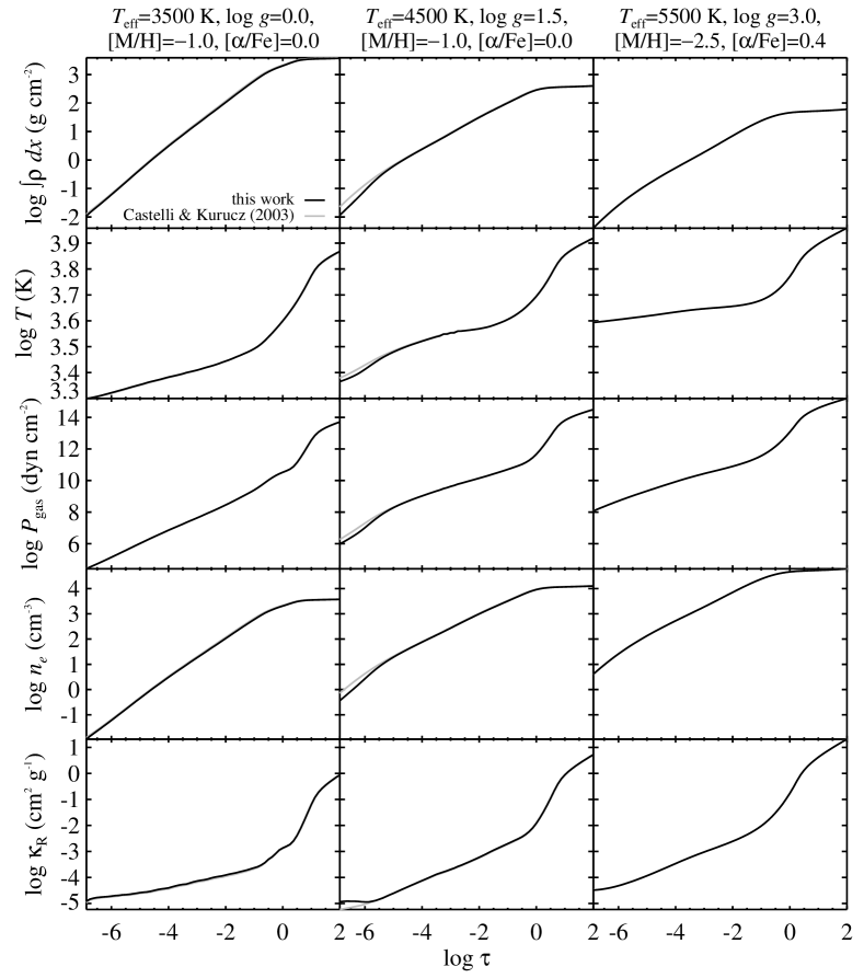
Figure 1: ATLAS9 model atmospheres computed here (black) compared to the ATLAS9 model atmospheres with the same parameters computed by Castelli & Kurucz (2003, gray). The black and gray lines overlap for much of this figure. Each column shows a different star whose parameters are given at the top of the column. The five rows show the mass depth ($\int\rho\,dx$), temperature ($T$), gas pressure ($P_{\rm gas}$), electron number density ($n_{e}$), and Rosseland mean opacity ($\kappa_{\rm R}$) as a function of the logarithm of optical depth ($\log\tau$).

The grid (Table 1) of plane-parallel model atmospheres in local thermodynamic equilibrium (LTE) was computed with Kurucz’s (1993a) DFSYNTHE, KAPPA9, and ATLAS9 codes ported into Linux (Sbordone et al., 2004; Sbordone, 2005) and compiled with the Intel Fortran compiler 11.1. All computations were performed in serial on 256 processors at the University of California Santa Cruz Pleiades Linux computing cluster. The compositions of the ODFs were the scaled solar abundances of Anders & Grevesse (1989) except that the abundance of iron was $12+\log\epsilon(\mathrm{Fe})=7.52$. The $\alpha$ elements O, Ne, Mg, Si, S, Ar, Ca, and Ti were additionally scaled by the parameter [$\alpha$/Fe].

The starting point for an ATLAS9 model atmosphere is an ODF. ODFs were computed in a manner identical to Castelli & Kurucz (2003) except for the elemental composition. In summary, DFSYNTHE (described by Castelli, 2005) was used to generate an ODF at each point in the stellar parameter grid. F. Castelli’s scripts (http://wwwuser.oat.ts.astro.it/castelli/) were employed for this purpose. These scripts compute ODFs at lower and higher effective temperatures than the grid presented here, but keeping the file formats consistent with Castelli’s scripts simplified later steps in computing the model atmospheres. The lists of atomic and some molecular (including H₂, HD, CH, C₂, CN, CO, NH, OH, MgH, SiH, and SiO but not including TiO or H₂O) transitions were those of R. L. Kurucz, downloaded at http://wwwuser.oat.ts.astro.it/castelli/sources/dfsynthe.html. See Kurucz (1990) for details of the line lists. The molecular line lists for TiO and H₂O, downloaded at the same URL, were provided by Schwenke (1998) and Partridge & Schwenke (1997), respectively. The KAPPA9 code in the same software package as DFSYNTHE computed Rosseland mean opacities from the ODFs.

For consistency with Castelli & Kurucz’s (2003) grid of ATLAS9 atmospheres, convective overshooting was turned off, and the mixing length parameter for convection was $l/H_{p}=1.25$. For each combination of $T_{\rm{eff}}$, $\log g$, [M/H], and [$\alpha$/Fe], there are two atmospheres with two different values of microturbulent velocity, $\xi$. The values are the two velocities among 0, 1, 2, and 4 km s^-1 that bracket the microturbulent velocity appropriate for the star’s surface gravity (Equation 2 of Kirby et al. (2009)): $\xi~{}(\mathrm{km~{}s}^{-1})=2.13-0.23\,\log g$.

ATLAS9 requires an input model atmosphere as an initial guess. An ATLAS9 model atmosphere with similar $T_{\rm{eff}}$, $\log g$, and [M/H] from Castelli & Kurucz’s grid was used for this purpose. At least 30 iterations were computed for each stellar atmosphere. After 30 iterations, convergence was tested by examining the difference in the flux and flux derivative between the last two iterations. Infrequently, these differences exceeded 1% for the flux or 10% for the flux derivative. In these cases, a different initial model atmosphere was used as input for 30 new ATLAS9 iterations. If the resulting atmosphere was still not converged, additional iterations were computed until the convergence criteria were satisfied.

In very rare cases, it was not possible to achieve these criteria with any number of iterations. These atmospheres were left as is. Most of these atmospheres corresponded to very luminous, warm red giants ($6000~{}\mathrm{K}\leq T_{\rm eff}\leq 8000~{}\mathrm{K}$ and $0.0\leq\log g\leq 0.5$). These stars lose mass in winds, which violate ATLAS9’s assumption of hydrostatic equilibrium. Stars with these atmospheric parameters are exceptionally rare. Therefore, convergence problems in this region of the grid are unlikely to cause problems for real astrophysical applications. The model atmospheres for M dwarfs ($T_{\rm eff}\lesssim 4000$ K, $\log g\lesssim 3.5$) also violated the convergence criteria to a small degree in the outer layers, especially at $\rm{[Fe/H]}\lesssim-1$. M dwarf atmospheres have low electron densities and non-blackbody spectral energy distributions, which cause them to be out of statistical equilibrium (Schweitzer, 1999). The outer layers affect the strongest absorption lines, which are often formed out of LTE even for warmer and larger stars.

Figure 1 shows some example stellar atmospheres. The parameters for each atmosphere were chosen to lie near a 14 Gyr isochrone from the Victoria-Regina set of isochrones (VandenBerg et al., 2006). For all three models, the microturbulent velocity is $\xi=2~{}{\rm km~{}s}^{-1}$. The parameters plotted are those relevant to the generation of synthetic spectra. From top to bottom, they are the logarithms of the mass depth ($\int\rho\,dx$), temperature ($T$), gas pressure ($P_{\rm gas}$), electron number density ($n_{e}$), and Rosseland mean opacity ($\kappa_{\rm R}$). The independent variable is the logarithm of the optical depth. The Castelli & Kurucz (2003) models for identical stellar parameters are also shown in gray for comparison. Subtle differences between the two sets of atmospheres—most visible in the middle column of Figure 1—occur due to the slight differences in elemental composition and different criteria for convergence. The largest differences occur in the shallowest layers of the atmosphere, which are important only for the formation of the strongest saturated lines.

3 MOOG Synthetic Spectra

Figure 2: Examples of three synthetic spectra computed with MOOG. The stellar parameters and model atmospheres are identical to those shown in Figure 1.

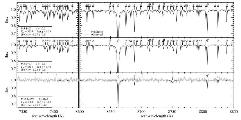
Figure 3: Examples of three synthetic spectra (black) compared to spectra observed with DEIMOS (gray). The synthetic spectra were interpolated in the grid in order to replicate the atmospheric parameters given in the legend at the left of each panel. The interpolated spectra were smoothed to match the resolution of the observed spectra ($R\approx 6500$). Some of the prominent stellar absorption lines are labeled with the abbreviation of the responsible element.

The grid of synthetic spectra was computed with the 2007 version of the plane-parallel, LTE code MOOG (Sneden, 1973). The code was modified to run in parallel via OpenMP on 256 processors on the Pleiades cluster. The parallelization was trivial, with different regions of the grid being computed simultaneously. Each spectrum was computed on a single processor. MOOG was also modified to output only the synthetic spectrum into an unformatted binary file. All other output was suppressed to save disk space and file access time. The normalized flux is computed every 0.02 Å from 6300 Å to 9100 Å. The units of the spectrum are such that the continuum is unity. The continuum shape is not computed. One spectrum is computed at each grid point.

MOOG requires two data tables as input: a model atmosphere and a line list. The model atmospheres were provided by the ATLAS9 atmospheres described in Section 2. However, the spectral grid was five times finer in the [M/H] dimension than the model atmospheres (see Table 1). Therefore, intermediate atmospheres spaced at 0.1 dex in [M/H] were generated by linear interpolation of the physical variables (not the logarithms of the physical values).

The microturbulent velocity chosen for each synthetic spectrum is a value appropriate for red giants (Equation 2 of Kirby et al. 2009): $\xi~{}(\mathrm{km~{}s}^{-1})=2.13-0.23\,\log g$. The atmosphere used to generate a spectrum was a linear interpolation between the two bracketing values of $\xi$. This linear interpolation was performed in conjunction with linear interpolation in [M/H], where necessary.

Kirby, Guhathakurta, & Sneden (2008) gave the complete line list, but the version used here has been modified according to Kirby et al. (2009). The original line list contained atomic lines from the Vienna Atomic Line Database (VALD, Kupka et al., 1999), molecular lines from Kurucz (1992), and hyperfine atomic lines from Kurucz (1993b). Oscillator strengths were modified to match observed line strengths in Arcturus and the Sun. Kirby et al. (2009) replaced the oscillator strengths ($\log gf$) for some Fe I lines with the values of Fuhr & Wiese (2006). For those Fe I lines not shared with Fuhr & Wiese (2006), 0.13 dex was subtracted from $\log gf$. The only molecules in the line list are CN, C₂, and MgH. The opacity for almost every line is considered only within 1 Å of the line’s central wavelength. Some lines are considered at every wavelength in the spectrum. These are H$\alpha$, the hydrogen Paschen series redward of 8370 Å, the Ca II triplet at 8498, 8542, and 8662 Å, and Mg I $\lambda 8807$.

Figure 2 shows 100 Å (7900–8000 Å) of the synthetic spectra computed from the model atmospheres shown in Figure 1. The full spectral range is 63 times what is shown. The abundances used to compute the line strengths are completely consistent with the abundances used to compute the model atmospheres.

Figure 3 shows synthetic spectra compared to spectra observed with the Keck/DEIMOS medium-resolution spectrograph. Kirby et al. (2010) obtained these spectra. These stars were chosen to have atmospheric parameters fairly close to those shown in Figures 1 and 2. The stars are red giants in the globular clusters M5 and M15. The atmospheric parameters for the synthetic spectra are given in the legend at the left of each panel (measured by Kirby et al., 2010). The synthetic spectra were linearly interpolated, pixel by pixel, to reproduce the measured atmospheric parameters. Finally, the synthetic spectral resolution has been degraded to match the DEIMOS instrumental resolution. In the spectrograph configuration used, profiles of unresolved lines have $\rm{FWHM}\approx 1.2$ Å almost independent of wavelength. Therefore, the resolving power is $R\approx 6200$ at 7400 Å and $R\approx 6700$ at 8700 Å.

The grid of synthetic spectra has several shortcomings, some of which are enumerated here.

1. The only molecules included are CN, C₂, and MgH. The number of TiO lines makes including them in the spectra computationally prohibitive. Therefore, cool, metal-rich stars are not modeled well in this grid. In reality, their spectra have TiO features that become extremely strong as the temperature decreases and metallicity increases.

2. Strong lines are not modeled well, mostly due to non-LTE effects. For example, Figure 3 clearly shows that the observed wings and core of the Ca II $\lambda 8662$ line are much stronger than in the synthetic spectrum.

3. Although a relation between microturbulent velocity and surface gravity has been established, not all stars obey this trend. In fact, the relation that Kirby et al. (2009) adopted was based only on red giants. The relation is not appropriate for most subgiants and dwarfs. The user is strongly cautioned against using any synthetic spectra with $\log g>3.5$ without verifying that the microturbulent velocity is appropriate for the specific star under consideration.

4 Online Data Access

The grids of model atmospheres and synthetic spectra may be obtained at the VizieR online catalogue service (Ochsenbein et al., 2000) at the following URL: http://vizier.u-strasbg.fr/viz-bin/VizieR?-source=VI/134. The user has two options to access the catalog. First, the catalog may be accessed either through the VizieR online interface, which includes an option to plot the synthetic spectra in a web browser. Second, one or both of the grids may be downloaded via FTP or HTTP. The compressed file sizes are 310 MB for the atmospheres and 46 GB for the spectra.

References

- Anders & Grevesse (1989) Anders, E., & Grevesse, N. 1989, Geochim. Cosmochim. Acta, 53, 197
- Castelli (2005) Castelli, F. 2005, MSAIS, 8, 34
- Castelli & Kurucz (2003) Castelli, F., & Kurucz, R. L. 2003, Modelling of Stellar Atmospheres, 210, 20P (astro-ph/0405087)
- Coelho et al. (2005) Coelho, P., Barbuy, B., Meléndez, J., Schiavon, R. P., & Castilho, B. V. 2005, A&A, 443, 735
- Frebel et al. (2010) Frebel, A., Simon, J. D., Geha, M., & Willman, B. 2010, ApJ, 708, 560
- Fuhr & Wiese (2006) Fuhr, J. R., & Wiese, W. L. 2006, Journal of Physical and Chemical Reference Data, 35, 1669
- Grevesse & Sauval (1998) Grevesse, N., & Sauval, A. J. 1998, Space Sci. Rev., 85, 161
- Kirby et al. (2009) Kirby, E. N., Guhathakurta, P., Bolte, M., Sneden, C., & Geha, M. C. 2009, ApJ, 705, 328
- Kirby et al. (2008) Kirby, E. N., Guhathakurta, P., & Sneden, C. 2008, ApJ, 682, 1217
- Kirby et al. (2010) Kirby, E. N., et al. 2010, ApJS, 191, 352
- Kupka et al. (1999) Kupka, F., Piskunov, N., Ryabchikova, T. A., Stempels, H. C., & Weiss, W. W. 1999, A&AS, 138, 119
- Kurucz (1970) Kurucz, R. L. 1970, SAO Special Report, 309
- Kurucz (1990) Kurucz, R. L. 1990, in NATO ASI C Ser., Stellar Atmospheres: Beyond Classical Models, ed. L. Crivellari, I. Hubený, & D. G. Hammer (Dordrecht: Kluwer), 441 Proc. 341: Stellar Atmospheres - Beyond Classical Models, 441
- Kurucz (1992) Kurucz, R. L. 1992, Revista Mexicana de Astronomia y Astrofisica, vol. 23, 23, 45
- Kurucz (1993a) Kurucz, R. L. 1993a, ATLAS9 Stellar Atmosphere Programs and 2 km/s grid. Kurucz CD-ROM No. 13. Cambridge, Mass.: Smithsonian Astrophysical Observatory, 1993, 13
- Kurucz (1993b) Kurucz, R. L. 1993b, Physica Scripta Volume T, 47, 110
- Letarte et al. (2010) Letarte, B., et al. 2010, A&A, 523, A17
- Mihalas (1965) Mihalas, D. 1965, ApJS, 9, 321
- Munari et al. (2005) Munari, U., Sordo, R., Castelli, F., & Zwitter, T. 2005, A&A, 442, 1127
- Ochsenbein et al. (2000) Ochsenbein, F., Bauer, P., & Marcout, J. 2000, A&AS, 143, 23
- Palacios et al. (2010) Palacios, A., Gebran, M., Josselin, E., Martins, F., Plez, B., Belmas, M., & Lèbre, A. 2010, A&A, 516, A13
- Partridge & Schwenke (1997) Partridge, H., & Schwenke, D. W., 1997, J. Chem. Phys., 106, 4618
- Sbordone (2005) Sbordone, L. 2005, MSAIS, 8, 61
- Sbordone et al. (2004) Sbordone, L., Bonifacio, P., Castelli, F., & Kurucz, R. L. 2004, MSAIS, 5, 93
- Schweitzer (1999) Schweitzer, A. 1999, Ph.D. Thesis, Landessternwarte Heidelberg/Königstuhl
- Schwenke (1998) Schwenke, D. W. 1998, Faraday Discussions, 109, 321
- Sneden (1973) Sneden, C. A. 1973, Ph.D. Thesis, University of Texas at Austin
- Strom & Avrett (1965) Strom, S. E., & Avrett, E. H. 1965, ApJS, 12, 1
- Strom & Kurucz (1966) Strom, S. E., & Kurucz, R. L. 1966, AJ, 71, 181
- VandenBerg et al. (2006) VandenBerg, D. A., Bergbusch, P. A., & Dowler, P. D. 2006, ApJS, 162, 375