Suzaku observations of the HMXB 1A 1118$-$61

Abstract

We present broad band analysis of the Be/X-ray transient 1A 1118$-$61 by Suzaku at the peak of its 3rd observed outburst in January 2009 and 2 weeks later when the source flux had decayed by an order of magnitude. The continuum was modeled with a cutoffpl model as well as a compTT model, with both cases requiring an additional black body component at lower energies. We confirm the detection of a cyclotron line at $\sim$ 55 keV and discuss the possibility of a first harmonic at $\sim$ 110 keV. Pulse profile comparisons show a change in the profile structure at lower energies, an indication for possible changes in the accretion geometry. Phase resolved spectroscopy in the outburst data show a change in the continuum throughout the pulse period. The decrease in the CRSF centroid energy also indicates that the viewing angle on the accretion column is changing throughout the pulse period.

1. Introduction

The Be/X-ray binary transient 1A 1118$-$61 was serendipitously discovered during an observation of the nearby binary system Cen X$-$3, when an outburst was detected in December of 1974 by the Ariel-5 satellite (Eyles et al., 1975). A second, similar outburst occured in January of 1992 and was observed by the Burst and Transient Source Experiment on the Compton Gamma Ray observatory CGRO/BATSE (Coe et al., 1994). The measured peak flux was $\sim 150$ mCrab for the 20-100 keV energy range, similar to the 1974 outburst. The source showed an elevated emission throughout the next $\sim 30$ days after the decay of the main outburst (see Coe et al., 1994, Fig. 1). The third and most recent outburst occurred on 2009, January 4 and was detected by the Swift Burst Alert Telescope BAT (Mangano et al., 2009; Mangano, 2009). It reached a peak flux of $\sim 500$ mCrab in the 15-50 keV energy band. This last outburst was monitored with Swift and the Rossi X-ray Timing Explorer (RXTE) as well as with two long Suzaku pointings and one observation with INTEGRAL during a flaring episode $\sim 50$  days after the peak of the main outburst (Leyder, Walter & Lubinski, 2009).

Pulsations with a period of $405.3\pm 0.6$ s were observed during the 1974 outburst and were initially attributed to the orbital period of two compact objects (Ives, Sanford & Bell Burnell, 1975). Shortly afterwards it was suggested that the period stems from a slow rotation of the neutron star (NS) itself (Fabian, 1975). During the 1992 outburst pulsations with a period of $\sim 406.5$ s were detected up to 100 keV, showing a broad, asymmetric, single peak pulse profile above the lowest BATSE energy of 20 keV. The pulse period decreased throughout the decline of the outburst with a rate of $\sim-0.016$ s/day and it appeared constant at $\sim 406.35$ s for the time of the elevated emission. During the 2009 outburst a similar period evolution was observed with RXTE resulting in a pulse period of $P_{\text{spin}}=407.719$ s, and $\dot{P}_{\text{spin}}=-4.6\times 10^{-7}$ s/s $\approx-0.04$ s/day (Doroshenko et al., 2010). Furthermore, the lower energies showed a more complex pulse profile with two peaks below an energy of $\sim 10$ keV. Due to the short duration of the Suzaku observations with respect to the pulse period, the derived RXTE values are used for determining the pulse profile and phase resolved spectra in this paper.

The optical counterpart was identified as the Be-star Hen 3$-$640/Wray 793 by Chevalier & Ilovaisky (1975) and classified as an O9.5IV-Ve star with strong Balmer emission lines indicating an extended envelope by Janot-Pacheco, Ilovaisky & Chevalier (1981). The overall spectrum was found to be similar to other known Be/X-ray transients, such as X$-$Per and A 0535+26 (Villada, Giovannelli & Polcaro, 1992, and references therein). The distance was estimated to be $5\pm 2$ kpc (Janot-Pacheco, Ilovaisky & Chevalier, 1981) and was confirmed by Coe & Payne (1985), along with the spectral type classification, using UV observations of the source. EXOSAT observed X-ray emission from 1A 1118$-$61 between outbursts (Motch et al., 1988), thus indicating a continuous low level of accretion. Rutledge et al. (2007) reported on pulsations in the low luminosity state observed with Chandra, making it only the third known HMXB transient after A 0535+26 and 4U 1145-619 for which this behavior has been observed.

A study of the $H_{\alpha}$ emission line before and during the 1994 outburst (Coe et al., 1994) showed a strong correlation between its strength and the observed X-ray activity, indicating the existence of a very large disk around the star. The fluctuation of the equivalent width of $H_{\alpha}$ indicated possible instabilities in the disk, which were enhanced when the star passes through the periastrion. The analysis of the UV continuum and line spectra has indicated that the photospheric emission from the Be star was not affected by the X-ray radiation, similar to the case of A 0535+26 (de Loore et al., 1984).

Until recently, the orbital period of 1A 1118$-$61 was not measured and assumed values were of the order of 350 days, based on the $P_{spin}-P_{orb}$ relation (Corbet, 1986), and $\sim 585$ days based on the equivalent width of the $H_{\alpha}$ line (Reig, Fabregat & Coe, 1997). Staubert et al. (2010) analyzed the pulse arrival time in RXTE data throughout the 2009 outburst and established an orbital period of $\sim 24$ days with a very circular orbit around the Be-companion.

Spectral fitting during the 1974 outburst indicated a variable power law index, where the lowest value was $\sim 0.9$ during the peak of the outburst, and $\sim 1.1$ before and after (Ives, Sanford & Bell Burnell, 1975). Coe et al. (1994) described the 1992 CGRO/BATSE data with a single-temperature, optically-thin, thermal bremsstrahlung (OTTB) with a temperature of 15 keV. Due to the different energy ranges of the instruments and the fact that pulse$-$off-pulse data have been used, these results can not be directly compared with the 1974 observation.

In the 2009 outburst Doroshenko et al. (2010) discovered a cyclotron resonance scattering feature (CRSF) at $\sim 55$ keV. CRSFs can be used to deduce the strength of the magnetic field at the pole region of the NS and have been observed in multiple sources at energies from $\sim 15$ keV up to $\sim 50$ keV (Coburn et al., 2002).

Suzaku observed 1A 1118$-$61 twice in 2009, once during the peak of the outburst and again $\sim 13$ days later when the flux had returned to a level slightly above the quiescent state. In this paper we will present the first detailed 0.7-200 keV broad band spectrum for this source, confirming the detection of a CRSF at $\sim 55$ keV. The paper is divided as follows: Section 2 describes the data accumulation and extraction; Section 3 presents the broad band phase averaged spectra for the outburst (0.7–200 keV) and for the second observation (0.7$-$70 keV), and discusses the CRSF and Fe-Line complex; Section 4 compares energy resolved pulse profiles for both observations and discusses the phase resolved analysis for the outburst data; finally Sections 5 and 6 present a discussion of our observations and summarize our findings.

Figure 1.— Swift/BAT lightcurve during the 1A 1118$-$61 outburst. The dashed lines mark the Suzaku observation as well as 2009 Jan 1.

2. Observation and Data Reduction

A sudden increase in activity of 1A 1118$-$61 was detected with the Swift/BAT instrument on January 4th, 2009 (Mangano et al., 2009). The count rate increased steadily until January 15th when it reached the maximum value of $\sim 500$ mCrab and then decayed until January 27th where it showed a low emission level with periods of flaring (Leyder, Walter & Lubinski, 2009) until mid March and then returned to quiescence (see Fig. 1). Suzaku observed 1A 1118$-$61 during the peak of the outburst on January 15th, 2009 (MJD 54846.5, ObsID 403049010) with both of its main instruments: the X-ray Imaging Spectrometer (XIS; Mitsuda et al., 2007) and the Hard X-ray Detector (HXD; Takahashi et al., 2007). A second observation was performed on January 28th, 2009 (MJD 54859.2, ObsID 403050010), $\sim 13$ days after the main outburst, at the beginning of the period of elevated emission.

Both observations were performed using the HXD nominal pointing to minimize the pile-up fraction in the XIS instruments and to enhance the HXD sensitivity for a possible CRSF detection. Of the four original XIS instruments only XIS 0, 1 and 3 were functional during the observing time. XIS 0 and 3 are both front illuminated (FI) CCDs and XIS 1 is a back illuminated (BI) CCD. To reduce pile-up, the XIS instruments were operated with the 1/4 window option with a readout time of 2 s and the burst option with only 1 s accumulation time for each readout cycle, reducing the exposure time for the XIS instruments by 50%. The data were taken in the $3\times 3$ and $5\times 5$ editing modes which were then combined for the final spectral analysis.

For the extraction the Suzaku FTOOLS version 16 (part of HEASOFT 6.9) was used. The unfiltered XIS data were reprocessed with caldb20090402 and then screened with the standard selection criteria as described in the ABC guide. Each detector and editing mode combination was extracted independently and individual response matrices and effective area files were created. For the final spectra the data from both FI detectors were combined (XIS 0 and 3) and the response matrices and effective areas were weighted according to the accumulated exposure time of the different modes. The XIS data were grouped so that the minimum number of channels per energy bin corresponded to at least the half width half maximum of the spectral resolution, i.e. grouped by 8, 12, 14, 16, 18, 20, 22 channels starting at 0.5, 1, 2, 3, 4, 5, 6, and 7 keV, respectively (Nowak, priv. com).

For the HXD data the Suzaku team provided the tuned PIN non X-ray background (NXB). Following the ABC Guide the cosmic X-ray background (CXB) was simulated and the exposure time was adjusted in both backgrounds by the prescribed factor of 10. The PIN data were grouped so that at least 100 events were detected in each spectral bin.

GSO data were extracted using the FTOOL hxdpi with the newest gain calibration file from April, 2010. The NXB background files version 2.4 created by the Suzaku HXD instrument team were used. The data were then binned to 64 bins according to the Suzaku homepage. GSO data in the range 70$-$200 keV were used in the spectral analysis.

These selection criteria resulted in $\sim$ 25 ks exposure time for each XIS instrument and $\sim$ 49 ks for the HXD instruments in the first observation. The second observation had an exposure of $\sim$ 21 ks and $\sim$ 29 ks for the XIS and HXD instruments, respectively.

2.1. Pileup correction

For bright sources, such as 1A 1118$-$61 during the outburst, a strong pileup is expected. Following the description provided at http://space.mit.edu/ASC/software/suzaku/ the S-lang routine aeattcor.sl was used to improve the attitude correction file and the point spread function of the events. Then the tool pile_estimate.sl was applied to produce a 2 dimensional map of the pileup fraction. The maximum values for pileup fractions were 10% and 15% for XIS0, 15% and 16% for XIS1, and 18% and 21% for XIS3 for the $3\times 3$ and $5\times 5$ editing modes, respectively. Regions with a pileup fraction above 5% were excluded from the extraction for each individual source event file. For the second observation the calculated maximum pileup fractions were ¡ 5% and no regions had to be excluded for the extraction.

3. Phase averaged spectrum

For the outburst observation we extracted broad band XIS spectra for 0.7$-$12 keV (0.7$-$10 keV for the BI XIS1), PIN spectra for 12–70 keV and GSO spectra for 70–200 keV. For the second observation the GSO spectrum was not well constrained and therefore was not included in the analysis. The final model included the Galactic and intrinsic absorption, a continuum that steepened at higher energies, an iron line complex, and a CRSF. Excessive low energy flux was modeled with a black body component. In addition a 10 keV absorption feature was required in the outburst observation.

The Galactic column density was modeled with a single photon absorption (phabs) component, where the column density was confined between 1.1 and 1.4 $\times 10^{22}$ cm^-2. The value determined by the NASA $N_{\text{H}}$ Tool for 1A 1118$-$61 is $1.22\times 10^{22}$ cm^-2. The $N_{\text{H}}$ value was left free in the fits for the first observation. For the second observation the values showed larger error bars with the cutoffpl model and had to be fixed when using a compTT model. The intrinsic column density was modeled with the partially covered photon absorption model pcfabs to take the flux at lower energies (¡1 keV) into account. All modeling was performed using the wilm abundances (Wilms, Allen & McCray, 2000) with the vern cross-sections (Verner et al., 1996). The continuum was modeled using a power law with an exponential cutoff (cutoffpl). Using a power law with a Fermi-Dirac (FD) cutoff, one of the empirical models often applied to accretion powered pulsars, resulted in a cutoff energy of $\sim 0$, making the FD cutoff effectively a cutoffpl, where the variable $E_{\text{cut}}$ actually reflects the folding energy of the model. The additional 10 keV feature was modeled using a negative, broad ($\sigma=1-2$ keV) Gaussian component. Such a feature has been previously observed in different sources and it is believed to stem from an improper modeling of the continuum (see §6.4 in Coburn et al., 2002). More recent examples of such a feature are, e.g. 4U1907+09 (Rivers et al., 2010) and Cen X$-$3 (Suchy et al., 2008). Although this feature sometimes is described as a broad emission line, e.g. Suchy et al. (2008), in this case a negative Gaussian line at $\sim$10 keV fits best. When including this line in the overall best fit, the $\chi^{2}$/dofs (degrees of freedom) decreased from 1173 / 477 to the best fit value of 678 / 474, respectively. Due to the small differences in the instrument response, all detectors were coupled with a normalization constant, which was set to 1 for the combined XIS 03 detectors. The final model is of the form const*phabs*pcfabs*(cutoffpl*gabs+ 2*Gauss${}_{\text{Fe}}$)+Gauss${}_{\text{10\,keV}}$+3*Gauss${}_{\text{Cal}}$. The best fit parameters are mentioned in the text and partially summarized in Table 1.

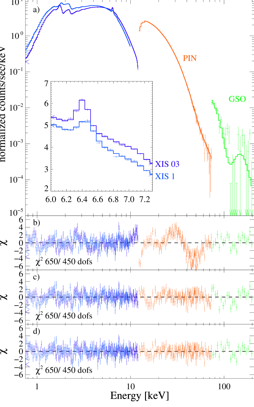
Figure 2.— Broad band phase averaged spectrum of the outburst observation using the cutoffpl model. The residuals are shown without CRSF (b), with one CRSF at 55 keV (c) and with the second CRSF at 112 keV. The Inset shows the Fe line region and the best fit model for XIS1 and XIS 03.

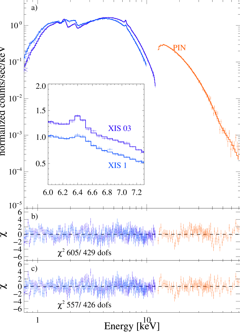
Figure 3.— Broad band phase averaged spectrum of the second observation using the cutoffpl model. Only XIS and PIN data were used. Residuals without a CRSF (b) and with one CRSF at $\sim 47$ keV. The Inset shows the Fe line region and the best fit model for XIS1 and XIS 03.

Table 1Phase averaged spectral parameter. Model described in the text.

Parameter	Cutoffpl			Parameter	CompTT
	Outbursta	2nd Obs.	2nd Obs, free CRSF		Outburst	2nd Obs.
phabs $N_{\text{H}}[10^{22}$/cm2]	$1.34^{+0.01}_{-0.01}$	$1.34$ frozen	$1.43^{+0.14}_{-0.13}$		$1.28^{+0.03}_{-0.02}$	$1.28$ frozen
pcfabs $N_{\text{H}}[10^{22}$/cm2]	$11.2^{+0.2}_{-0.3}$	$13.5^{+0.4}_{-0.4}$	$13.6^{+0.5}_{-0.5}$		$12.00^{+0.4}_{-0.5}$	$15.1^{+0.1}_{-0.7}$
covering fract.	$0.66^{+0.01}_{-0.01}$	$0.71^{+0.01}_{-0.01}$	$0.71^{+0.01}_{-0.01}$		$0.71^{+0.01}_{-0.01}$	$0.76^{+0.01}_{-0.01}$
blackbody kT [keV]	$0.51^{+0.01}_{-0.003}$	$0.15^{+0.01}_{-0.01}$	$0.15^{+0.01}_{-0.01}$		$0.53^{+0.01}_{-0.01}$	$0.17^{+0.01}_{+0.01}$
blackbody norm $[10^{-3}]$	$7.3^{+0.4}_{-0.2}$	$2.2^{+0.2}_{-0.03}$	$2.85^{+1.67}_{-1.22}$		$12.8^{+1.1}_{-0.9}$	$2.89^{+0.03}_{-0.02}$
$E_{\text{cut}}$ [keV]	$18.7^{+0.2}_{-0.2}$	$26.3^{+3.0}_{-2.5}$	$24.7^{+1.8}_{-1.6}$	compTT T0 [keV]	$1.34^{+0.04}_{-0.05}$	$0.44^{+0.06}_{-0.04}$
$\Gamma$	$0.350^{+0.022}_{-0.004}$	$1.02^{+0.04}_{-0.04}$	$1.01^{+0.03}_{-0.03}$	compTT kT [keV]	$7.6^{+0.3}_{-0.3}$	$182^{+158}_{-96}$
$A_{\text{pl}}[10^{-2}]^{\dagger}$	$9.55^{+0.02}_{-0.03}$	$5.8^{+0.3}_{-0.3}$	$5.7^{+0.3}_{-0.3}$	compTT $\tau_{\text{p}}$	$6.00^{+0.19}_{-0.18}$	$0.68^{+1.33}_{-0.26}$
				compTT norm†	$0.096^{+0.003}_{-0.003}$	$0.002^{+0.004}_{-0.001}$
$E_{\text{CRSF}}$ [keV]	$58.2^{+0.8}_{-0.4}$	$58.2$ frozen	$47.4^{+3.2}_{-2.3}$		$54.5^{+2.4}_{-2.1}$	$54.5$ frozen
$\sigma_{\text{CRSF}}$ [keV]	$14.1^{+3.5}_{-3.1}$	$14.1$ frozen	$5.7^{+2.0}_{-1.7}$		$10.3^{+3.6}_{-0.1}$	$10.3$ frozen
$\tau_{\text{CRSF}}$	$60.1^{+5.9}_{-1.5}$	$15.4^{+6.4}_{-6.3}$	$6.0^{+3.0}_{-2.1}$		$23.6^{+10.4}_{-6.9}$	$27.1^{+3.2}_{-3.0}$
$E_{\text{Fe~{}K}_{\alpha}}$ [keV]	$6.414^{+0.006}_{-0.002}$	$6.42^{+0.01}_{-0.01}$	$6.42^{+0.01}_{-0.01}$		$6.42^{+0.01}_{-0.01}$	$6.42^{+0.01}_{-0.01}$
$E_{\text{Fe~{}K}_{\beta}}$ [keV]	$7.13^{+0.03}_{-0.03}$	$7.13$ frozen	7.13 frozen		$7.13^{+0.03}_{-0.03}$	$7.13$ frozen
Eq. Width Kα / Kβ [eV]	$51^{+4}_{-4}/8^{+3}_{-3}$	$46^{+10}_{-10}/8^{+2}_{-2}$	$46^{+10}_{-10}/8^{+2}_{-2}$		$51^{+4}_{-4}/10^{+3}_{-3}$	$49^{+10}_{-10}/11^{+9}_{-9}$
Flux${}_{2-10\,\text{keV}}[10^{36}$ ergs/sec ]‡	8.79	1.72	1.72		9.15	1.72
C${}_{\text{XIS1}}$/C${}_{\text{PIN}}$/C${}_{\text{GSO}}$	0.98 / 1.10 / 0.82	1.02 / 1.01/–	1.02/1.01/–		0.99/ 1.18 / 1.10	0.95/ 1.00/–
$\chi^{2}$/dofs	678 / 474	574 / 431	567 / 428		680 / 474	567 / 428

Note. — ^a Best fit values including first harmonic at $\sim 110$ keV, see text for details. $\dagger$ Units in Photons keV^-1 cm^-2 s^-1, $\ddagger$ unabsorbed flux using a distance of 5 kpc

A second approach for the continuum was initiated by Doroshenko et al. (2010) using the Comptonization model compTT developed by Titarchuk & Hua (1995) instead of the cutoffpl model. The parameters of the compTT were again left independent between the FI XIS03 and the BI XIS1, but only small differences could be observed. The negative Gaussian at 10 keV was not necessary for this model. When comparing the spectral parameters in the outburst between these two models, i.e. CRSF, $N_{\text{H}}$ and the spectral lines, to the previously described cutoffpl, the values were consistent.

A comparison of the compTT values, such as the photon seed temperature $T_{0}$, the plasma Temperature $kT_{\text{e}}$ or the optical depth $\tau_{p}$ showed consistency between the spectra of the outburst as seen by Suzaku and RXTE (Doroshenko et al., 2010).

When comparing the outburst spectrum with the second observation, significant changes in the continuum parameters are observed. In the cutoffpl model the power law index softened from $0.350^{+0.022}_{-0.004}$ to $1.01^{+0.03}_{-0.03}$. The cutoff energy $E_{\text{cut}}$ increased from $18.7^{+0.2}_{-0.2}$ keV during the outburst to $24.7^{+1.8}_{-1.6}$ keV in the second observation. The temperature of the additional black body decreased from $0.51^{+0.01}_{-0.003}$ keV to $0.15^{+0.01}_{-0.01}$ keV after the outburst. The intrinsic column density and covering fraction increased both from $11.2^{+0.2}_{-0.3}\times 10^{22}$ cm^-2 and $0.66^{+0.01}_{-0.01}$ in the outburst to $13.6^{+0.5}_{-0.5}\times 10^{22}$ cm^-2 and $0.71^{+0.01}_{-0.01}$ in the second observation.

In the compTT model the changes between the two observations were similar. The intrinsic column density and black body values were consistent with the values obtained with the cutoffpl model, where the intrinsic column density is $12.0^{+0.4}_{-0.5}\times 10^{22}$ cm^-2 and $15.1^{+0.1}_{-0.7}\times 10^{22}$ cm^-2 and the covering fraction is $0.71^{+0.01}_{-0.01}$ and $0.76^{+0.01}_{-0.01}$ for the outburst and the second observation, respectively. When establishing the errors for the other spectral parameters of the continuum, these values had to be frozen to avoid a drift into an unreasonable part of the parameter space. The black body temperature declined from $0.53^{+0.01}_{-0.01}$ keV to $0.17^{+0.01}_{-0.01}$ keV, similar values as in the cutoffpl model. The compTT values changed significantly between the two observations. The photon seed temperature decreased from $1.34^{+0.04}_{-0.05}$ keV to $0.44^{+0.06}_{-0.04}$ keV. The electron plasma temperature $kT_{\text{e}}$ increased from $7.6^{+0.3}_{-0.3}$ keV to $182^{+158}_{-96}$ keV, whereas the optical depth of the plasma $\tau_{p}$ decreased from $6.00^{+0.19}_{-0.18}$ to $0.68^{+1.33}_{-0.26}$. This behavior reflects the known negative $kT_{\text{e}}$ and $\tau_{p}$ correlation (see Section 5.2).

3.1. Fe line component

An Fe K_α emission component was detected at $6.414^{+0.006}_{-0.002}$ keV in the outburst data (see Fig. 2, Inset), as well as at $6.42^{+0.01}_{-0.01}$ keV in the 2nd observation (see Fig. 3, Inset). For the best fit values the centroid energies of XIS03 and XIS 1 were left independent, due to a known shift in the energy calibration. Although the centroid energies for XIS1 generally show a slightly lower (30 eV) energy than the other XIS instruments, our XIS1data instrument actually showed a 20-30 eV higher centroid energy. Residuals at $\sim 7$ keV were observed and were modeled with an additional Gaussian line with a best-fit energy of $7.13\pm 0.03$ keV, indicating the existence of an Fe K_β line. The width $\sigma$ of the Fe K_β line was set to the Fe K_α line value, and the normalization was left independent. The obtained value for the K_β normalization was consistent with the expected 12% of the K_α normalization. In the second observation the second line was very weak and its parameters could not be properly constrained. In this case the line centroid was frozen at the outburst value of 7.13 keV. The width was again coupled with the Fe K_α value. The residuals decreased from $\chi^{2}=721$ for 477 dofs to the overall best fit values of $678$ for 474 dofs, including two CRSFs, when the Fe K_β line was included and an F-test showed only a $2.8\times 10^{-6}$ probability that this improvement is of a statistical nature. Another possibility for modeling the observed residuals at $\sim 7$ keV is the addition of an Fe K-edge, located at 7.1 keV. When including the edge, the improvement is only marginal ($\chi^{2}$ of 712 for 474 dofs) and the best fit energy is $\sim 7.6$ keV. Freezing the energy to the value of 7.1 keV did not improve the fit. The remaining residuals indicated that an additional Fe K_β line would still be necessary. The measured energies of the Fe K_α and K_β lines were slightly higher than the expected laboratory values, but still in the same order of magnitude of the energy scale uncertainties of the instrument ( $\sim\pm$ 20 eV @ 6 keV according to the ABC guide).

Comparing the equivalent widths (EQWs) of the Fe K_α and K_β lines in the two observations showed no significant change during the outburst. The Fe K_α line showed an EQW of $51\pm 4$ eV for both models, whereas the Fe K_β line showed an EQW of $8\pm 3$ eV for the cutoffpl model and $10\pm 3$ eV in the compTT model. For the second observation, the Fe K_α EQWs were $46\pm 10$ eV and $49\pm 10$ eV, and the K_β EQWs were $8\pm 2$ eV and $11\pm 9$ eV for the cutoffpl and compTT models, respectively. The similarity of the Fe line EQW between both observations indicates that the source of the Fe lines is near to the source of the continuum (see discussion).

3.2. Cyclotron resonance scattering feature

In the burst observation a strong residual at $\sim 50$ keV was observed in the HXD (Fig. 2, b). When including a CRSF-like feature with a Gaussian optical depth profile (gabs) the best fit was obtained with a centroid energy of $58.2^{+0.8}_{-0.4}$ keV, significantly improving the $\chi^{2}$ from 1728 with 480 dofs to 752 for 477 dofs for the cutoffpl model, confirming the discovery of the CRSF in the RXTE data by Doroshenko et al. (2010). The width of the line was $14.1^{+3.5}_{-3.1}$ keV and the optical depth $\tau$ was $60.1^{+5.9}_{-1.5}$. Using the compTT model, similar values for $E_{\text{cyc}}$ and $\sigma$ were obtained for the outburst data. In this case the optical depth was found to be $23.6^{+10.4}_{-6.9}$.

In the cutoffpl model, a second absorption line, using the gabs model, in the GSO data of the outburst spectrum at $\sim 110$ keV improved the $\chi^{2}$ to 678 with 474 dofs (see Fig. 2c). An F-test probability of $0.144$ indicates that the line may not be significantly detected. However, an increase of the GSO Non X-ray Background (NXB) by 1 or 2% decreased the GSO counts to a non-detectable value. Another possible systematic effect is the decay of the ¹⁵³Gd instrumental line, which is activated when the satellite passes through the south atlantic anomaly (SAA), and thus creating a background line at $\sim 150$ keV. This could impose a deviation at $\sim 110$ keV if not accurately represented in the modeled background. Therefore caution is advised when interpreting this feature.

In the lower luminosity observation only an indication of the fundamental CRSF was observed (see Fig. 3). The line was fitted in 2 steps, where first the centroid energy and width were fixed to the outburst values, and the optical depth was left as a free parameter. With the addition of this CRSF, the cutoffpl model improved slightly from a $\chi^{2}$/dofs of 605 / 432 to 574 / 431 with an optical depth of $\tau=15.4^{+0.64}_{-0.63}$. In the second step, the CRSF parameters were left free and the centroid energy decreased to $47.4^{+3.2}_{-2.3}$ keV, whereas the optical depth decreased to $\tau=6.0^{+3.0}_{-2.1}$ and the width decreased to $\sigma=5.7^{+2.0}_{-1.7}$ keV. With a $\chi^{2}$/dofs of 567 / 428 the best fit improved further (see Tab. 1 for details). To test the significance of the CRSF in the second observation, 100 000 PIN spectra were Monte Carlo simulated using the null hypothesis approach where a spectrum, including Poisson noise, was created using the best fit parameters without an CRSF line. The simulated spectra were then fitted with a continuum model and an additional gabs absorption line to test how often such a line could be detected in the spectral noise. The width was constrained to a value of $\sigma$ between 3.5 keV and 8.5 keV, so that neither very small features nor broad parts of the continuum were modeled. Out of the 100 000 simulations, 42% of the best fit results showed a non-zero value of $\tau$. When comparing the simulated $\tau$ distribution with the best fit result of $\tau=6.0^{+3.0}_{-2.1}$, $\sim 96$% of all simulated fits showed a value between 0 and the measured value. When taking the errors of the measured data into account ($\tau<3.9$) the number is reduced to $\sim 90$%.

For the compTT model, the addition of the fundamental CRSF with the frozen energy and width created residuals in the $10-20$ keV range, which could be significantly reduced by decoupling the optical depth of the compTT model in the PIN data from the XIS data. The best fit optical depth of the CRSF line was $27.1^{+3.2}_{-3.0}$ changing the $\chi^{2}$ / dof values from 639 / 429 to 567 / 428, respectively. When leaving the CRSF parameters free, the width of the CRSF increased to $>30$ keV, making it part of the continuum and tampering with the results. Freezing the CRSF parameters to the values obtained with the cutoffpl model did not result in a satisfactory overall fit.

An alternative approach to describe the CRSF is to replace the gabs model with the XSPEC model cyclabs (Mihara et al., 1990), described by the resonance energy $E_{\text{res}}$, the resonance width $\sigma_{\text{res}}$ and the resonance depth $\tau_{\text{res}}$. Using this model does not improve the fits significantly, and actually results in a slightly worse $\chi^{2}/$dofs value of 782 / 475 for the outburst data. Note that in the case of cyclabs the ratio between the energy of the fundamental and first harmonic line are fixed to 2, resulting in 1 more degree of freedom. The observed $E_{\text{res}}$ of $49.5^{+0.8}_{-0.8}$ keV is of the order of $\sim 20$% below the centroid energy obtained with the gabs model. This discrepancy stems from the use of a different calculation of the line energy and is of the order of $10-20$ % lower than the measured gabs energy (see Nakajima et al., 2010, for details). No significant changes in the continuum parameters have been observed when using the cyclabs model. A width of $\sigma_{\text{res}}=19.4^{+2.8}_{-1.3}$ keV and a depth of $\tau_{\text{res}}=1.45^{+0.10}_{-0.06}$ are obtained for the outburst observation. In the second observation the resonance energy shows a slight decrease ($E_{\text{res}}=45.7^{+2.3}_{-2.0}$ keV), and only slightly smaller than the gabs values. These results reflect again the difficulty of constraining the possible CRSF parameters in the second observation. The width and depth, $\sigma_{\text{res}}=5.6^{+3.7}_{-2.4}$ keV and $\tau_{\text{res}}=0.46^{+0.19}_{-0.14}$, are consistent with the gabs result showing a decrease in width and depth for both observations.

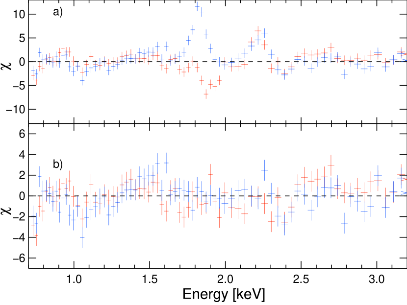
Figure 4.— Instrumental residuals at lower energies for XIS 1 (blue) and XIS 03 (red) with the cutoffpl model. a) shows the clearly apparent lines are the Au K_α line at $\sim 2.1$ keV and the Si K_α line at $\sim 1.8$ keV. Additionally a possible Ni K_α line at $\sim 0.9$ which improves the fit slightly. b) shows the best fit residuals when the lines are included.

3.3. Low energy calibration issues

Strong residuals at lower energies, i.e. between 1.5 and 2.5 keV (see Fig. 4) were observed in both data sets. A comparison with known background properties of the Suzaku/XIS instrument (Yamaguchi et al., 2006) showed that these features are identical to the known instrumental Si K_α and Au K_α lines, located at 1.74 keV and 2.12 keV, respectively. In many observations of bright sources, e.g. 4U 1907+07 (Rivers et al., 2010) and LMC X$-$3 (Kubota et al., 2010), these energy bands are explicitly excluded. In this case, modeling these lines with two Gaussian emission features was sufficient to minimize the residuals and improve the $\chi^{2}$/dofs from 1295 / 483 (without the lines) to the best fit value of 678 / 474. Note that the Au K_α line at $\sim 2.1$ keV could be described by the same Gaussian emission line at $2.21\pm 0.01$ keV for both FI and BI XIS instruments, whereas the Si K_α line appears as an emission line for the BI XIS1 at $1.82\pm 0.01$ keV (Fig. 4, blue) and a negative Gaussian line at $1.89\pm 0.01$ keV for the FI XIS 03 combination (Fig. 4, red), indicating that for the FI instrument the line is either over-subtracted or not properly energy calibrated, leading to a dip in the spectrum. By using two independent lines at 1.89 keV (FI) and 1.82 keV (BI) the residuals can be well described. An additional Gaussian component at $0.93^{+0.01}_{-0.02}$ keV, located close to the Ni K edge at 0.897 keV, slightly improves the residuals ($\chi^{2}$/dofs of 731 / 477 without the line, compared to the best-fit value of 678 / 474) This improvement indicates a possible systematic error of the calibration at lower energies for bright sources. This line is not very pronounced and can be omitted when using the compTT model.

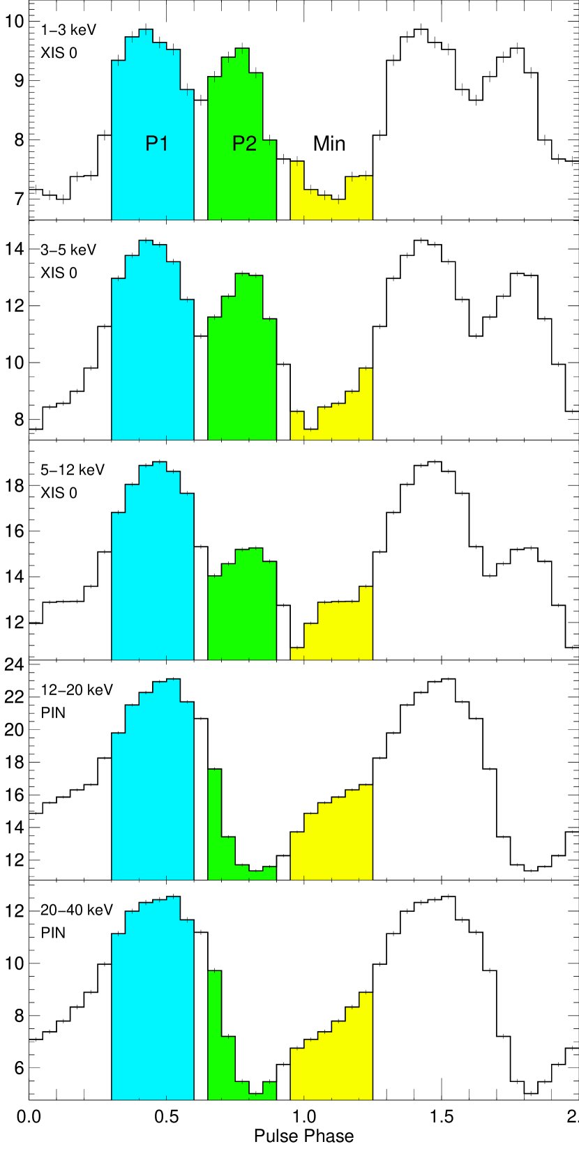
Figure 5.— XIS and PIN pulse profiles for different energy bands for the outburst observation. P1, P2 and MIN indicate the regions used for the phase resolved spectral analysis.

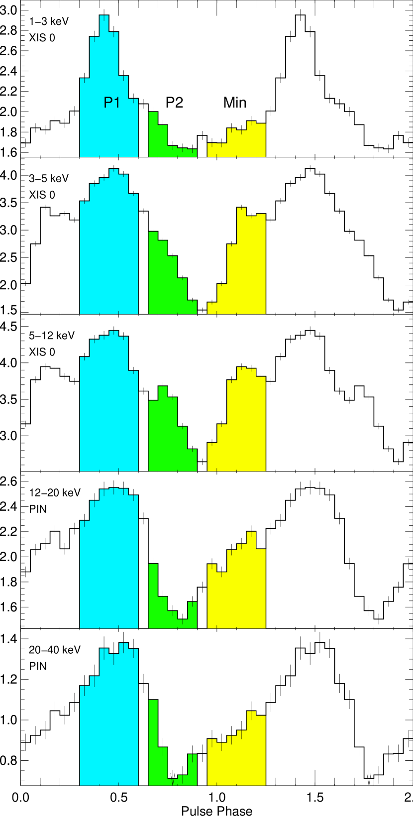
Figure 6.— Same as Fig. 5 for the second observation. The highlighted regions indicate the same phase bins as in the outburst observation for a direct comparison

4. Phase resolved analysis

For a phase resolved analysis the XIS and PIN data of both observations were folded with the RXTE determined pulse period from Doroshenko et al. (2010) of $P_{\text{spin}}=407.719$ s, $\dot{P}_{\text{spin}}=-4.6\times 10^{-7}$ s/s and the MJD epoch of 54841.62. Pulse profiles with 20 phase bins were created for five different energy bands in the $1-10$ keV energy range for XIS and $12-40$ keV energy range for PIN for both observations (Fig. 5 and Fig. 6). The statistical quality of the GSO data precluded the creation of pulse profiles and further spectral analysis.

During the outburst, the pulse profile consisted of two peaks, where the main peak (P1, pulse phase $0.3-0.6$) stayed dominant throughout all energy bands and became broader towards higher energies (Fig. 5). The second peak (P2, pulse phase $0.65-0.9$) disappeared at energies above $\sim 10$ keV, consistent with the RXTE observations by Doroshenko et al. (2010). The third region in Fig. 5 indicates the minimum of the pulse profile (MIN, pulse phase $0.95-1.25$), as determined from the lower energies of the XIS instrument.

In comparison, the pulse profile of the second observation (Fig. 6) showed a similar Peak P1 throughout the whole energy band, although narrower at lower energies. No second peak was observed at the position of P2, although a small “bump” in the $5-12$ keV energy range was still visible. At lower energies, i.e. for the $3-5$ and $5-12$ keV energy band, a small peak showed up on the opposite site of P1, the pulse phase where the minimum was defined in the outburst data.

4.1. Phase resolved spectroscopy

Spectra were extracted for three different pulse phases throughout the outburst: P1, P2 and MIN. XIS and PIN spectra were used and the same XIS grouping as in the phase averaged data was applied. The PIN data was again grouped to include at least 100 counts per spectral bin. The same spectral model was used as in the phase averaged analysis and the best-fit results are summarized in Table 2. In all pulse phases the CRSF component was visible in the spectra. Throughout the pulse phase the best-fit values for the galactic and intrinsic $N_{\text{H}}$ values did not change significantly. Note that in both models a slight decrease of the covering fraction during P2 can be observed.

Table 2Phase resolved outburst spectral parameters. Same models as in Table 1

Parameter	Cutoffpl			Parameter	CompTT
	Peak 1	Peak 2	Minimum		Peak 1	Peak 2	Minimum
phabs $N_{\text{H}}[10^{22}$/cm2]	$1.35^{+0.02}_{-0.03}$	$1.38^{+0.03}_{-0.01}$	$1.21^{+0.04}_{-0.04}$		$1.28^{+0.04}_{-0.05}$	$1.22^{+0.6}_{-0.5}$	$1.20^{+0.04}_{-0.05}$
pcfabs $N_{\text{H}}[10^{22}$/cm2]	$11.1^{+0.8}_{-0.5}$	$10.6^{+0.4}_{-0.2}$	$11.7^{+1.1}_{-1.1}$		$11.6^{+0.8}_{-0.8}$	$11.0^{+0.9}_{-1.0}$	$12.16^{+1.09}_{-0.89}$
covering fract.	$0.66^{+0.03}_{-0.03}$	$0.52^{+0.1}_{-0.02}$	$0.67^{+0.05}_{-0.05}$		$0.70^{+0.03}_{-0.04}$	$0.58^{+0.6}_{-0.7}$	$0.70^{+0.04}_{-0.05}$
blackbody kT [keV]	$0.52^{+0.03}_{-0.02}$	$0.58^{+0.01}_{-0.02}$	$0.50^{+0.02}_{-0.02}$		$0.54^{+0.03}_{-0.02}$	$0.59^{+0.03}_{-0.03}$	$0.52^{+0.03}_{-0.02}$
blackbody norm $[10^{-3}]^{\dagger}$	$7.0^{+1.0}_{-1.6}$	$2.3^{+0.6}_{-0.4}$	$8.1^{+1.7}_{-0.7}$		$12.3^{+1.7}_{-1.9}$	$8.9^{+1.6}_{-1.6}$	$10.1^{+1.6}_{-1.4}$
$E_{\text{cut}}$ [keV]	$29.5^{+7.2}_{-3.2}$	$18.3^{+0.8}_{-0.4}$	$10.7^{+1.3}_{-0.9}$	compTT T0 [keV]	$1.31^{+0.10}_{-0.07}$	$1.41^{+0.04}_{-0.05}$	$1.48^{+0.11}_{-0.07}$
$\Gamma$	$0.42^{+0.06}_{-0.04}$	$0.56^{+0.04}_{-0.02}$	$-0.13^{+0.09}_{-0.08}$	compTT kT [keV]	$7.67^{+1.39}_{-0.38}$	$11.91^{+9.06}_{-2.77}$	$6.79^{+0.75}_{-0.21}$
$A_{\text{pl}}^{\dagger}$	$0.12^{+0.01}_{-0.01}$	$0.14^{+0.01}_{-0.00}$	$0.04^{+0.004}_{-0.004}$	compTT $\tau_{\text{p}}$	$6.31^{+0.31}_{-0.40}$	$4.00^{+0.47}_{-0.45}$	$6.60^{+0.38}_{-0.62}$
				compTT norm †	$0.11^{+0.01}_{-0.01}$	$0.05^{+0.02}_{-0.01}$	$0.08^{+0.01}_{-0.01}$
$E_{\text{CRSF}}$ [keV]	$66.6^{+0.9}_{-2.3}$	$55.5^{+0.5}_{-0.7}$	$52.8^{+2.9}_{-2.0}$		$57.9^{+8.7}_{-4.2}$	$57.7^{+2.0}_{-4.1}$	$51.0^{+4.9}_{-2.4}$
$\sigma_{\text{CRSF}}$ [keV]	$19.2^{+3.6}_{-2.7}$	$11.4^{+0.3}_{-0.2}$	$9.3^{+2.5}_{-1.6}$		$13.5^{+15.5}_{-3.4}$	$14.9^{+2.9}_{-3.1}$	$9.0^{+4.6}_{-2.0}$
$\tau_{\text{CRSF}}$	$130.8^{+7.0}_{-19.6}$	$44.1^{+2.3}_{-3.3}$	$22.7^{+14.6}_{-7.3}$		$25.6^{+45.4}_{-12.3}$	$79.5^{+64.8}_{-40.2}$	$13.5^{+20.4}_{-4.7}$
$E_{\text{Fe~{}K}\alpha}$ [keV]	$6.41^{+0.01}_{-0.01}$	$6.41^{+0.01}_{-0.01}$	$6.42^{+0.01}_{-0.01}$		$6.41^{+0.01}_{-0.01}$	$6.41^{+0.01}_{-0.01}$	$6.42^{+0.01}_{-0.01}$
$E_{\text{Fe~{}K}\beta}$ [keV]	$7.16^{+0.05}_{-0.05}$	$7.08^{+0.06}_{-0.06}$	$7.09^{+014}_{-0.11}$		$7.16^{+0.04}_{-0.05}$	$7.09^{+0.06}_{-0.05}$	$7.12^{+0.14}_{-0.12}$
Eq. Width Kα / Kβ [eV]	$37^{+9}_{-6}/7^{+7}_{-7}$	$59^{+8}_{-9}/11^{+9}_{-9}$	$64^{+9}_{-9}/8^{+7}_{-8}$		$39^{+5}_{-6}/10^{+7}_{-7}$	$58^{+7}_{-4}/13^{+7}_{-8}$	$62^{+9}_{-8}/8^{+9}_{-8}$
Flux${}_{2-10\,\text{keV}}[10^{36}$ ergs/sec ]‡	10.5	8.14	7.5
C${}_{\text{XIS1}}$/C${}_{\text{PIN}}$	0.98 / 1.1	0.97 / 1.04	0.99/1.16		1.04 / 1.23	0.99 / 1.19	1.08 / 1.23
$\chi^{2}$/dofs	$498/431$	$508/420$	474 / 427		528 / 438	492 / 423	542 / 430

Note. — $\dagger$ Units in Photons keV^-1 cm^-2 s^-1, $\ddagger$ unabsorbed flux using a distance of 5 kpc

The most significant variation in the cutoffpl model was that of the cutoff energy $E_{\text{cut}}$ which decreased from $29.5^{+7.2}_{-3.2}$ keV in P1, to $18.3^{+0.8}_{-0.4}$ keV in P2 and down to $10.7^{+1.3}_{-0.9}$ keV in MIN. At the same time the power law index $\Gamma$ varied from $0.42^{+0.06}_{-0.04}$ (P1), to $0.56^{+0.04}_{-0.02}$ (P2), and to $-0.13^{+0.09}_{-0.08}$ for MIN. In the three phases the CRSF centroid energy changed from $66.6^{+0.9}_{-2.3}$ keV in P1, and declined to $55.5^{+0.5}_{-0.7}$ keV throughout P2, and $52.8^{+2.9}_{-2.0}$ keV for MIN. The CRSF width declined from $19.2^{+3.6}_{-2.7}$ keV in P1 to $11.4^{+0.3}_{-0.2}$ keV in P2, and to $9.3^{+2.5}_{-1.6}$  keV in MIN.

For the compTT model most parameters did not change throughout the pulse profile. The observed increase in the plasma temperature and the decrease of the optical depth $\tau_{\text{p}}$ is a known systematic anti-correlation (see discussion). As with the phase averaged data, the CRSF did not show the same changes throughout the pulse profile, as in the cutoffpl model. The best-fit values for the CRSF centroid energy were $57.9^{+8.7}_{-4.2}$ keV for P1, $57.7^{+2.0}_{-4.1}$ keV for P2, and $51.0^{+4.9}_{-2.4}$ keV for MIN, and the widths were $13.5^{+15.5}_{-3.4}$ keV,$14.9^{+2.9}_{-3.1}$ keV, and $9.0^{+4.6}_{-2.0}$ keV for P1, P2 and MIN, respectively. Fe K_α and Fe K_β energies were consistent with $\sim 6.4$ keV and $\sim 7.1$ keV, similar to the cutoffpl values.

5. Discussion

This paper presents an analysis of the two Suzaku observations of the Be/X-Ray binary 1A 1118$-$61 during the peak of its outburst in 2009, January and $\sim 13$ days later. A CRSF, detected with RXTE at $\sim 55$ keV, could be observed in both observations, although the significance is lower in the second observation. An Fe K_β line at $7.13$ keV has been observed in addition to the strong, narrow Fe K_α line at 6.4 keV. The broad band continuum was modeled with the empirical cutoffpl model, including an additional 10 keV systematic component to improve the residuals. Softening of the power law index $\Gamma$ between peak and decay had been observed in an earlier outburst and could be confirmed. The Comptonization model compTT, where the 10 keV component was not needed, has also been applied. The pulse profiles at lower energies changed from a two peaked to a single peaked profile between both observations. Phase resolved spectral analysis was performed for both observations and the same models as in the phase averaged analysis were applied.

5.1. Outburst behavior

The third observed outburst of 1A 1118$-$61 follows a pattern similar to the second outburst from 1992, i.e. a strong peak lasting $\sim 3$ weeks and an elevated level of emission up to 6 weeks afterwards. The time between outbursts was in both cases $\sim 6200$ days, corresponding to $\sim 17$ years, indicating that the outburst behavior could be periodic on very long time scales. The proposed orbital periods are $\sim 350$ days (Corbet, 1986), $\sim 58$ days (Reig, Fabregat & Coe, 1997). and most recently 24 days established by Staubert et al. (2010) using the delay in pulse arrival time of RXTE monitoring observations throughout this outburst. Using the latter method the Suzaku light curves are in full agreement with the RXTE results (Staubert, priv. comm). A period of 24 days would put 1A 1118$-61$ in the wind accretor region on the “Corbet” diagram (Corbet, 1986), making it a very unique source for a Be system.

A very similar scenario was introduced by Villada et al. (1999), who monitored the $H_{\alpha}$/$H_{\beta}$ emission before and after the second outburst and proposed that the optical companion, Hen $3-640$, has an extended large envelope where a weak interaction with the NS can occur. In the scenario of Villada et al. (1999), the NS is orbiting the O star in an environment with gradually increasing density, until a steady accretion disk is created and the X-ray flux suddenly increases. The sudden increase in the accretion material would provide the torque on the NS to produce the observed changes in the pulse period. The surrounding material is then swept out in a short time and the system returns to quiescence. According to Villada et al. (1999), an interval of 17 years between the outbursts is a reasonable time scale to accumulate enough material between the outbursts.

5.2. Cyclotron features

In the outburst, a CRSF has been observed at $\sim 55$ keV and the parameters are consistent with the RXTE data (Doroshenko et al., 2010). A CRSF in the second observation is expected but can not be confirmed with sufficient significance in the established data.

CRSFs are generated by electrons with energies close to the ones determined by the discrete energy states of the Landau levels being excited to higher levels followed by de-excitation emitting a photon. In this process, photons from the accretion column above the magnetic poles with a resonant cyclotron line energy, are resonantly scattered out of the line of sight creating an absorption line-like feature. These features provide a direct measure of the magnetic field strength close to the NS surface, where the fundamental cyclotron energy is given by

$$E_{\text{cyc}}=\frac{\hbar eB}{m_{e}c}\frac{1}{1+z}=\frac{11.6\text{\,keV}}{1+z}\times B_{12},$$ (1)

where $B_{12}$ is the magnetic field strength near the NS surface in units of $10^{12}$ Gauss and $z$ is the gravitational redshift. Assuming a typical NS mass of 1.4 $M_{\odot}$ and NS radius of 10 km gives $z=0.3$. For 1A 1118$-$61 the CRSF at $\sim$ 55 keV corresponds to a magnetic field of $\sim 6.4\times 10^{12}$ Gauss, making it, together with the $\sim 50$ keV line of A 0535+26, one of the strongest observed magnetic fields on an accreting neutron star in a binary system.

A possible feature in the residuals at $\sim 110$ keV could indicate the existence of a first harmonic line, as observed in multiple sources, such as 4U 0115+63 (Heindl et al., 1999), 4U 1907+09 (Cusumano et al., 1998; Makishima et al., 1999) and Vela X$-$1 (Makishima et al., 1999; Kreykenbohm et al., 2002). Including a gabs line at this energy does not significantly improve the fit, though a ¹⁵³Gd instrumental line at $\sim 150$ keV, which is due to electron-capture (Kokubun et al., 2007), as well as possible systematic uncertainties in the background weaken the significance of the detection further.

Assuming that the observed width of the CRSF is due to the Doppler broadening of the electrons responsible for the resonances, one can estimate the inferred plasma temperature in the CRSF region using equation 4.1.28 from Meszaros (1992):

$$\Delta\omega_{\text{D}}=\omega_{\text{Cyc}}\left(\frac{2kT}{m_{e}c^{2}}\right)^{1/2}|{\text{cos}(\Theta})|,$$ (2)

where $\Delta\omega_{\text{D}}$ corresponds to the CRSF FWHM which is calculated from $\sigma_{\text{Cyc}}$, $\omega_{\text{Cyc}}$ is equivalent to the CRSF centroid energy $E_{\text{Cyc}}$ and $\Theta$ is the angle between magnetic field lines and the line of sight. With $\text{cos}(\Theta)=1$ the lower limits for the plasma temperature are $kT\approx 20.8$ keV for the cutoffpl model and $kT\approx 12.6$ keV for the compTT model when using the values from Tab. 1.

Although the existence of a CRSF in the second observation is only marginal, it is very likely that such a line exists at lower luminosities. Luminosity dependance of CRSFs have been observed in multiple other binary system. In Be-Binaries, such as V 0332+53, 4U 0115+63, and X 0331+53, where Tsygankov et al. (2006) and Nakajima et al. (2006, 2010) found a negative correlation between the CRSF centroid energy and the luminosity of the source for luminosities approaching the Eddington luminosity. Staubert et al. (2007) on the other hand found a positive CRSF$-$luminosity correlation in the low mass X-ray binary Her X$-$1 for luminosities far below the Eddington luminosity.

The type of correlation seems to depend on whether the observed luminosity is above or below the Eddington luminosity. When the luminosity is above the Eddington luminosity, the infalling protons start to interact before they are part of the accretion column and a “shock front” region, where the CRSF most likely occurs, is created. With increasing luminosity, the proton interaction occurs farther away from the NS surface, where the magnetic field is lower and therefore the observed CRSF is seen at lower energies. Below the Eddington luminosity, the proton interaction does not occur above the accretion column but is part of it. When the luminosity increases, the accretion “pressure” increases as well and the region where the CRSF is created is pressed closer to the NS surface, where the magnetic field is higher. This results in a positive CRSF-luminosity correlation, as observed in Her X$-$1.

The flux levels (Tab. 1) obtained for both observations showed that the first observation is most likely above, and the second observation is definitely below the Eddington luminosity of the system, so that an anti-correlation between CRSF centroid energy and luminosity are expected.

5.3. Continuum comparison

When comparing both observations, changes in the broad band continuum parameters were observed. During the 1974 outburst Ives, Sanford & Bell Burnell (1975) observed a harder spectrum in the peak compared to later observation. Looking at the cutoffpl model, the Suzaku data showed a similar behavior with a very hard spectrum (power law index $\Gamma=0.35$) at the luminosity peak, and a much softer power law index of $\Gamma\sim 1$ in the second observation. Note also that the cutoff/folding energy increased with declining luminosity. A similar behavior has been observed in a number of different HMXB transients, such as A 0535+26 (Caballero, 2009) and V 0332+53 (Mowlavi et al., 2006). This is in contrast to EXO 2030+375 (Reynolds, Parmar & White, 1993), where the observed folding energy increased with lower luminosity. Soong et al. (1990) interpreted this parameter in phase resolved results and concluded that the folding energy reflects a change of the viewing angle on the accretion column, which allows a deeper look into the emission region and therefore directly correlates with the observed electron plasma temperature. The change observed in the phase averaged observations follows a similar reasoning, and at lower luminosities the emission region is closer to the NS, where the observed plasma temperatures are expected to be higher.

A comparison of compTT parameters between Suzaku and RXTE (Doroshenko et al., 2010) showed consistent results for the spectral parameters in the outburst. In contrast to the RXTE results, the observed column density $N_{\text{H}}$ is higher and consistent with the results obtained by the cutoffpl model. The main difference between these results and the RXTE data lies in the use of a combined Galactic and intrinsic column density and the additional need of a low energy black body, so that these values cannot be compared directly. Note that the RXTE/PCA instrument used in Doroshenko et al. (2010) is not sensitive to data below 3 keV and therefore a partial covering, as well as a black body component could not be modeled. Both, the black body temperature for the low energy excess and the photon seed temperature in the compTT model decreased by $\sim 1/3$ between outburst and the second observation, indicating a correlation between both parameters. A possible explanation is that the source of the compTT seed photons is the same as the soft excess modeled by the black body component. The observed change in the optical thickness indicates the the observed material is optically thick in the outburst and gets optically thinner for the second observation.

Although an increase in the plasma temperature of the compTT model was observed after the outburst, i.e., mainly consistent with the interpretation of the cutoffpl parameters, one has to be careful with a direct interpretation of the spectral parameter. The optical depth $\tau$ and the electron plasma temperature $kT_{\text{e}}$ show a very strong negative correlation (e.g. Wilms et al., 2006), and the best-fit values cannot be used directly for interpretation. Following the definition in Rybicki & Lightman (1979), the Compton $y$ parameter:

$$y=\frac{4kT_{\text{e}}}{m_{\text{e}}c^{2}}\text{max}(\tau,\tau^{2}),$$ (3)

can help in the physical interpretation. Reynolds & Nowak (2003) used the Compton $y$ parameter in the description of accretion disk coronae around black holes. A value of $y\approx 1$ or slightly higher means that the average emitted photon energy increases by an “amplification factor”, $A(y)\approx\text{exp}(y)$, and is referred to as “unsaturated inverse Comptonization”. For $y\gg 1$ the average photon energy reaches the thermal energy of the electrons. This case is called the “saturated inverse Comptonization”. Using $kT$ and $\tau_{p}$ results in $y=2.13\pm 0.2$ for the outburst data and $y=1^{+9}_{-0.7}$ for the second observation. Typical calculated values of $y$-parameters are smaller than 1, e.g., $\sim 0.5$ for Cyg X$-$1 (Reynolds & Nowak, 2003), $\sim 0.2$ for 4U 2206+54 (Torrejón et al., 2004), and $\sim 0.6$ for XV 1832$-$330 (Parmar et al., 2001). Note that the second observation is very badly constrained due to the large error bars on the electron plasma temperature and the optical depth and therefore cannot be used for interpretation. The $y$ parameter for the Suzaku outburst indicates that the system is in, or very close, to a “saturated inverse Comptonization” state.

5.4. Fe lines

In both observations an Fe K_α and Fe K_β emission line has been observed, where the Fe K${}_{\alpha}-$ Fe K_β normalization ratio of 12% is consistent with neutral material. The Fe K_α EQWs were $51\pm 4$ eV and $46\pm 10$ eV for the first and second observation, respectively, while at the same time the $5-7$ keV power law flux dropped from $6.50\pm 0.01\times 10^{-10}$ ergs cm^-2 s^-1 to $1.23\pm 0.01\pm\times 10^{-10}$ ergs cm^-2 s^-1. The relatively constant EQWs imply that the Fe line emitting region is relatively close to the source of ionizing flux, so that the observed Fe line intensity adapts quickly to the changing incident flux. The Fe line normalization was $1.79\pm 0.06\times 10^{-3}$ photons cm^-2 s^-1 and $3.15\pm 0.3\times 10^{-4}$ photons cm^-2 s^-1 for the respective observations. The ratios between Fe normalization and power law flux were consistent in both observations, $2.75\pm 0.10$ and $2.56\pm 0.27\times 10^{6}$ photons/ergs, reflecting the two calculated EQWs. Using the continuum flux difference and the time between observations, the calculated change in power law flux was $\sim 0.415\pm 0.001\times 10^{-10}$ ergs cm^-2 s^-1 per day in the 12.7 day period between the observations. A linear decrease could be assumed using the BAT data of Fig. 1. For the second observation, the Fe normalization was manually increased in XSPEC until the resulting EQW matched the upper limit of the measured EQW. This value corresponds to an Fe normalization of $\sim 3.9\times 10^{-4}$ photons cm^-2 s^-1, assuming the measured continuum given above for the second observation. Together with the previously calculated constant of $2.56\times 10^{6}$, a matching power law flux of $\sim 1.52$ could be calculated. Using this flux difference, together with the rate of change in the $5-7$ keV energy range, one can then determine a maximum time delay which would still preserve the observed EQW within errors. The calculated upper limit to the delay between the Fe and X-ray emission region is $\sim 0.7$ days. Note that this estimation is very simple and uncertainties from the orbital motion or from line of sight assumptions are not taken into account here.

5.5. Phase resolved description

1A 1118$-$61 shows a similar energy and luminosity pulse profile dependency as many other sources, e.g. 4U 0115+63 (Tsygankov et al., 2007), V 0332+53 (Tsygankov et al., 2006) and A 0535+26 (Caballero, 2009). In the outburst observation, the observed broad double peaked structure at lower energies changed to a single peak profile above 10 keV, where the main peak (P1) broadened slightly with increased energy and the secondary peak (P2) weakened. For the second observation, the pulse profile changed significantly. There was still a dominant primary peak at P1, although it is narrower in the lowest energy band. The secondary peak is only marginally indicated between $5-12$ keV (see Fig. 6) and absent in the other energy bands. On the other hand, between $3-12$ keV a small peak or extended shoulder could be observed preceding the primary peak.

To confirm the disappearance of the second peak, pulse fractions of the total counts of the P1/P2 regions were calculated for the indicated energy bands. The pulse fraction was defined as (P1${}_{\text{countrate}}-$P2${}_{\text{countrate}}$) / P2${}_{\text{countrate}}$ where the P1 and P2 regions are indicated in Fig. 5 and 6. Table 3 shows that the pulse fraction increases towards higher energies in the outburst data, typical for a weakening of the second pulse. In the second observation the values do not vary for the different energy bands, and the small peak in the $5-12$ keV band shows only a marginal smaller pulse fraction than in the other energy bands.

Table 3Pulse fractions for 1A 1118$-$61

Energy [keV]	Outburst	2nd Obs
$1-3$	0.26	0.73
$3-5$	0.31	0.90
$5-12$	0.48	0.53
$12-20$	1.00	0.78
$20-40$	1.19	0.83

Tsygankov et al. (2007) described similar profiles and proposed that a misalignment of the rotational and magnetic axes of the neutron star leads to the case where one accretion column is observed whole, whereas the second accretion column is partially screened by the NS surface so that only the softer photons, which are created in the higher regions of the accretion column, are observed. When the overall luminosity, and therefore accretion rate, decreases, the column height decreases and even the soft photons from the second pole are shielded. This behavior is in contrast to the variation observed in the cyclotron line production region, where the line forming region is closer to the NS surface at higher luminosities.

For a more physical picture gravitational effects, such as light bending, have to be taken into account when discussing pulse profiles (Kraus et al., 1995; Meszaros & Nagel, 1985). For a canonical NS with a mass of 1.4$M_{\odot}$ and a radius of 10 km the visible surface of a NS is 83%. With this increased surface visibility the pulsed flux from both hot spots is visible over a longer part of the pulse phase, and parts of the accretion column of the second peak are still visible, although that hot spot is on the far side of the NS. With decreasing luminosity, the hot spot size decreases and the visible fraction of the second accretion column disappears.

Pulse profile decomposition methods have been developed by Kraus et al. (1995), and have been applied to multiple sources, e.g. EXO 2030+375 (Sasaki et al., 2010) and A 0535+26 (Caballero, 2011). Under the assumption of a slightly distorted magnetic dipole, with this method it is possible to disentangle the contribution of the two emission regions, and constraints on the geometry of the pulsar and on its beam pattern can be obtained. The application of this method on the 1A1118 data presented here will be left for future work.

A more physical approach for a broad band spectrum has been introduced by Becker & Wolff (2007), using bulk and dynamical Comptonization of photons in the accretion column. First results on 4U 0115+63 have been promising (Ferrigno et al., 2009) and 1A 1118$-$61 is a good candidate for future tests. Schönherr et al. (2007) developed a new physical model for the CRSFs based on Monte Carlo simulations for the Green’s functions for the radiative transport through a homogeneous plasma, which had been successfully applied for different sources, e.g., Cen X-3 (Suchy et al., 2008). Due to advances in the overall code (Schwarm, 2007) the test of this model on this data set is beyond the scope of this paper.

6. Summary and Conclusions

In this paper we analyzed the broad band spectrum and pulse profiles of 1A 1118$-$61 during the peak of its third observed outburst and compared the results with a second observation which occurred $\sim 2$ weeks after the main peak. The time between outbursts is consistent with a continuous low level accretion mechanism as suggested by Villada et al. (1999). A CRSF during the outburst has been confirmed at $\sim 55$ keV indicating one of the highest known B-fields observed in HMXBs. In the second observation there is only a weak indication of a CRSF fundamental line. A change in the CRSF centroid energy with respect to luminosity would be expected and would help to understand the physical environment close to the NS surface. Variations of the CRSF can also be observed in the phase resolved spectroscopy of the outburst observation. The calculated $y$ parameters show that the inverse Comptonization during the outburst is very close to saturation. The ratio between the Fe K_α and Fe K_β normalization of $\sim 12\%$ shows that the emitting material is mostly neutral. Using the compTT model, one can deduce that the emitting material is optically thick during the outburst and optically thin in the second observation, although the known $kT-\tau$ correlation has to be considered. The pulse profile change for different energy bands and luminosities is similar to other observed HMXBs and can be explained with a misalignment of the rotation axis to the magnetic field axis. A change in the pulse profile shape with luminosity has been observed and indicates that the visibility of the second hot spot changes between the observations. Phase resolved analysis throughout the outburst also indicates a change in the observed magnetic field, which could be caused by different viewing angles onto the accretion column. Future work with a pulse deconvolution technique, as well as a more physical model will provide a better understanding of the involved physical processes.

References

- Becker & Wolff (2007) Becker, P. A., & Wolff, M. T., 2007, ApJ, 654, 435
- Caballero (2009) Caballero, I., 2009, Ph.D. thesis, IAAT University of Tuebingen
- Caballero (2011) Caballero, I., Kraus, U., Santangelo, A., Sasaki, M., Kretschmar, P., 2011, A&A, 526, A131
- Chevalier & Ilovaisky (1975) Chevalier, C., & Ilovaisky, S. A., 1975, IAU Circ, 2778, 1
- Coburn et al. (2002) Coburn, W., Heindl, W. A., Rothschild, R. E., Gruber, D. E., Kreykenbohm, I., Wilms, J., Kretschmar, P., & Staubert, R., 2002, ApJ, 580, 394
- Coe & Payne (1985) Coe, M. J., & Payne, B. J., 1985, Ap&SS, 109, 175
- Coe et al. (1994) Coe, M. J., et al., 1994, A&A, 289, 784
- Corbet (1986) Corbet, R. H. D., 1986, MNRAS, 220, 1047
- Cusumano et al. (1998) Cusumano, G., di Salvo, T., Burderi, L., Orlandini, M., Piraino, S., Robba, N., & Santangelo, A., 1998, A&A, 338, L79
- de Loore et al. (1984) de Loore, C., et al., 1984, A&A, 141, 279
- Doroshenko et al. (2010) Doroshenko, V., Suchy, S., Santangelo, A., Staubert, R., Kreykenbohm, I., Rothschild, R., Pottschmidt, K., & Wilms, J., A&A, 515, L1
- Eyles et al. (1975) Eyles, C. J., Skinner, G. K., Willmore, A. P., & Rosenberg, F. D., 1975, Nature, 254, 577
- Fabian (1975) Fabian, A. C., 1975, MNRAS, 173, 161
- Ferrigno et al. (2009) Ferrigno, C., Becker, P. A., Segreto, A., Mineo, T., & Santangelo, A., 2009, A&A, 498, 825
- Heindl et al. (1999) Heindl, W. A., Coburn, W., Gruber, D. E., Pelling, M. R., Rothschild, R. E., Wilms, J., Pottschmidt, K., & Staubert, R., 1999, ApJ Letter, 521, L49
- Ives, Sanford & Bell Burnell (1975) Ives, J. C., Sanford, P. W., & Bell Burnell, S. J., 1975, Nature, 25caba4, 578
- Janot-Pacheco, Ilovaisky & Chevalier (1981) Janot-Pacheco, E., Ilovaisky, S. A., & Chevalier, C., 1981, A&A, 99, 274
- Kokubun et al. (2007) Kokubun, M., et al., 2007, PASJ, 59, 53
- Kraus et al. (1995) Kraus, U., Nollert, H.-P., Ruder, H., & Riffert, H., 1995, ApJ., 450, 763
- Kreykenbohm et al. (2002) Kreykenbohm, I., Coburn, W., Wilms, J., Kretschmar, P., Staubert, R., Heindl, W. A., & Rothschild, R. E., 2002, A&A, 395, 129
- Kubota et al. (2010) Kubota, A., Done, C., Davis, S. W., Dotani, T., Mizuno, T., & Ueda, Y., 2010, ApJ, 714, 860
- Leyder, Walter & Lubinski (2009) Leyder, J., Walter, R., & Lubinski, P., 2009, The Astronomer’s Telegram, 1949, 1
- Makishima et al. (1999) Makishima, K. and Mihara, T. and Nagase, F. and Tanaka, Y., 1999, ApJ, 525, 978
- Mangano (2009) Mangano, V., 2009, The Astronomer’s Telegram, 1896, 1
- Mangano et al. (2009) Mangano, V., et al., 2009, GRB Coordinates Network, 8777, 1
- Meszaros & Nagel (1985) Meszaros, P., & Nagel, W., 1985, ApJ, 299, 138
- Meszaros (1992) Meszaros, P., 1992, High-Energy Radiation from Magnetized Neutron Stars, Chicago Press
- Mihara et al. (1990) Mihara, T., Makishima, K., Ohashi, T., Sakao, T., Tashiro, M., 1990, Nature, 346, 250
- Mitsuda et al. (2007) Mitsuda, K., et al., 2007, PASJ, 59, 1
- Motch et al. (1988) Motch, C., Pakull, M. W., Janot-Pacheco, E., & Mouchet, M., 1988, A&A, 201, 63
- Mowlavi et al. (2006) Mowlavi, N., et al., 2006, A&A, 451, 187
- Nakajima et al. (2006) Nakajima, M. and Mihara, T. and Makishima, K. and Niko, H., 2006, ApJ, 646, 1125
- Nakajima et al. (2010) Nakajima, M. and Mihara, T. and Makishima, K., 2010, ApJ, 710, 1755
- Parmar et al. (2001) Parmar, A. N., Oosterbroek, T., Sidoli, L., Stella, L., & Frontera, F., 2001, A&A, 380, 490
- Protassov et al. (2002) Protassov, R., van Dyk, D. A. , Connors, A., Kashyap, V. L., & Siemiginowska, A., 2002, ApJ, 571, 545
- Reig, Fabregat & Coe (1997) Reig, P., Fabregat, J., & Coe, M. J., 1997, A&A, 322, 193
- Reynolds, Parmar & White (1993) Reynolds, A. P., Parmar, A. N., & White, N. E., 1993, ApJ, 414, 302
- Reynolds & Nowak (2003) Reynolds, C. S., & Nowak, M. A., 2003, Phys. Reports , 377, 389
- Rivers et al. (2010) Rivers, E., et al., 2010, ApJ, 709, 179
- Rutledge et al. (2007) Rutledge, R. E., Bildsten, L., Brown, E. F., Chakrabarty, D., Pavlov, G. G., & Zavlin, V. E., 2007, ApJ, 658, 514
- Rybicki & Lightman (1979) Rybicki, G. B. & Lightman, A., 1979, Radiative processes in astrophysics, Wiley
- Sasaki et al. (2010) Sasaki, M., Klochkov, D., Kraus, U., Caballero, I., & Santangelo, A., 2010, A&A, 517, A8+
- Schönherr et al. (2007) Schönherr, G., Wilms, J., Kretschmar, P., Kreykenbohm, I., Santangelo, A., Rothschild, R. E., Coburn, W., & Staubert, R., 2007, A&A, 472, 353
- Schwarm (2007) Schwarm, F, 2010, Diploma thesis, Univ. Erlangen-Nuernberg.
- Soong et al. (1990) Soong, Y., Gruber, D. E., Peterson, L. E., & Rothschild, R. E., 1990, ApJ, 348, 641
- Staubert et al. (2010) Staubert, R., Pottschmidt, K., Doroshenko, V., Wilms, J., Suchy, S., Rothschild, R., & Santangelo, A., 2011, A&A, 527, A7
- Staubert et al. (2007) Staubert, R., Shakura, N. I., Postnov, K., Wilms, J., Rothschild, R. E., Coburn, W., Rodina, L., & Klochkov, D., 2007, A&A, 465, L25
- Suchy et al. (2008) Suchy, S., et al., 2008, ApJ, 675, 1487
- Takahashi et al. (2007) Takahashi, T., et al., 2007, PASJ, 59, 35
- Titarchuk & Hua (1995) Titarchuk, L., & Hua, X., 1995, ApJ, 452, 226
- Torrejón et al. (2004) Torrejón, J. M., Kreykenbohm, I., Orr, A., Titarchuk, L., & Negueruela, I., 2004, A&A, 423, 301
- Tsygankov et al. (2006) Tsygankov, S. S., Lutovinov, A. A., Churazov, E. M., & Sunyaev, R. A., 2006, MNRAS, 371, 19
- Tsygankov et al. (2007) Tsygankov, S. S., Lutovinov, A. A., Churazov, E. M., & Sunyaev, R. A., 2007, Astronomy Letters, 33, 368
- Verner et al. (1996) Verner, D. A., Ferland, G. J., Korista, K. T., & Yakovlev, D. G., 1996, ApJ, 465, 487
- Villada, Giovannelli & Polcaro (1992) Villada, M., Giovannelli, F., & Polcaro, V. F., 1992, A&A, 259, L1
- Villada et al. (1999) Villada, M., Rossi, C., Polcaro, V. F., & Giovannelli, F., 1999, A&A, 344, 277
- Wilms, Allen & McCray (2000) Wilms, J., Allen, A., & McCray, R., 2000, ApJ, 542, 914
- Wilms et al. (2006) Wilms, J., Nowak, M. A., Pottschmidt, K., Pooley, G. G., & Fritz, S., 2006, A&A, 447, 245
- Yamaguchi et al. (2006) Yamaguchi, H., et al., 2006, in SPIE Conference Series, Vol. 6266