MHV diagrams in twistor space and the twistor action
Abstract
MHV diagrams give an efficient Feynman diagram-like formalism for calculating gauge theory scattering amplitudes on momentum space. Although they arise as the Feynman diagrams from an action on twistor space in an axial gauge, the main ingredients were previously expressed only in momentum space and momentum twistor space. Here we show how the formalism can be elegantly derived and expressed entirely in twistor space. This brings out the underlying superconformal invariance of the framework (up to the choice of a reference twistor used to define the axial gauge) and makes the twistor support transparent. Our treatment is largely independent of signature, although we focus on Lorentz signature.
Starting from the super-Yang-Mills twistor action, we obtain the propagator for the anti-holomorphic Dolbeault-operator as a delta function imposing collinear support with the reference twistor defining the axial gauge. The MHV vertices are also expressed in terms of similar delta functions. We obtain concrete formulae for tree-level MHV diagrams as a product of MHV amplitudes with an R-invariant for each propagator; here the R-invariant manifests superconformal as opposed to dual-superconformal invariance. This gives the expected explicit support on lines linked by further lines associated to the propagators. The R-invariants arising correspond to those obtained in the dual conformal invariant momentum twistor version of the formalism, but differences arise in the specification of the boundary terms. Surprisingly, in this framework, some finite loop integrals can be performed as simply as those for tree diagrams.
1 Introduction
An important output of Witten’s twistor string theory [1] was the MHV diagram formalism [2, 3, 4]. This is a momentum space Feynman-diagram formalism for gauge theories that is much more efficient than standard ones. In this formalism, the propagators are the standard massless scalar propagators, , and the vertices are obtained from a simple off-shell extension of the Parke-Taylor formula [5, 6] for the ‘MHV’ amplitudes (these being, in our conventions, the tree amplitudes that have the maximal number of negative helicity external gluons but nevertheless being nontrivial, leaving just two of positive helicity). This formalism was shown to give the correct amplitudes at tree-level [7, 8, 9] and for 1-loop MHV [10]. It has also recently been expressed in momentum twistor space [11] where it was shown to give the correct planar momentum space loop integrand to all orders for supersymmetric theories which are cut-constructible [12]. We emphasize that this recent work in momentum twistor space [13] is distinct to that in ordinary twistor space as described in this paper. Momentum twistor space is essentially a new rational coordinatization of momentum space that brings out dual superconformal invariance and only applies to planar gauge theories (really one is computing a Wilson-loop there, not the S-matrix [14]). Amplitudes on twistor space are not locally related to those on momentum twistor space and have quite different analytic properties as we shall see. We remark also that the loop integrands that these studies concern are canonical and finite, but lead to infrared divergences in four-dimensions when integrated and then require regularization, though we will not address this major issue in this paper.
MHV diagrams were originally motivated from twistor-string theory. Twistor-string theory had already led to formulae for tree-level scattering amplitudes in Super-Yang-Mills (SYM) as a path-integral over curves in super twistor space [15, 16]. In these formulae, NkMHV amplitudes (i.e., those involving positive helicity gluons with the rest negative) correspond to the part of the amplitude supported on curves in twistor space of degree . Although it has not been possible to extend these ideas to loop amplitudes (conformal super-gravity corrupts the calculations beyond tree-level [17]) the MHV formalism is not obstructed in the same way and as noted above works to all loop orders at the level of the four-dimensional integrand. It was based on the idea that, instead of a connected degree curve, one could consider lines that are geometrically disconnected, but are joined by propagators [18]. This was expressed only loosely in twistor space, but has a well-defined momentum space diagram formalism.
The connection between classical Yang-Mills theory, twistor-string theory and the MHV formalism was subsequently understood in terms of twistor actions for supersymmetric gauge theories [19, 20, 21, 22] on twistor space (see [23, 24] for other approaches). These actions have greater gauge freedom than that on space-time; on one hand they reduce to the space-time actions non-peturbatively in one gauge. On the other, twistor actions can be gauge fixed in an axial gauge on twistor space that is inaccessible from space-time; the corresponding Feynman diagrams are then precisely the MHV diagrams [25]. Although this gave a field theory explanation of the origins of the MHV formalism in momentum space, it was not able to exploit the advantages that could have been hoped for from a twistorial formulation, such as making contact with ideas from twistor-string theory and being able to exploit the superconformal invariance of the twistor formulation to obtain a simpler and more natural formalism.
More recently however, there has been an emphasis on understanding amplitudes directly in twistor space rather than via a momentum space representation; in effect we consider the scattering of particles that are supported at a single twistor, an ‘elemental state’. The first systematic works [26, 27] (following on from some earlier works, particularly [28]) were based on Witten’s half-Fourier transform from momentum space to twistor space using the transform of the BCFW recursion relations [29, 30]. This required analytic continuation to split signature, which is unphysical, but avoided the need to worry about the cohomological nature of twistor wave functions. It led to a superconformally invariant formulation (up to some symmetry breaking signs) that clearly brought out the twistor support of the BCFW representations of the amplitudes [31, 32]. For example, terms in the BCFW decomposition of an NkMHV tree diagram are supported on configurations of lines containing loops (triangles for NMHV). These ideas led to a Grassmannian representation for the tree amplitudes and leading singularities [33, 34, 32].
In this paper we continue this investigation for the twistor representation of amplitudes arising from the MHV formalism. We obtain amplitudes directly in twistor space starting from the twistor action without referring to space-time or momentum space. We have also developed the technology further, using ideas from [34, 16, 14] to obtain a signature independent formulation that incorporates the cohomological nature of twistor wave functions whilst maintaining an explicit and superconformally invariant formulation up to the choices required for the axial gauge fixing. This is based on the use of distributional -forms in the multiple copies of twistor space. Although at first sight these might seem to go against the general holomorphic philosophy of twistor theory, there is no obstruction to basing the calculus on Čech cohomology that uses holomorphic functions as its representatives. However, there would then be more gauge freedom and complicated combinatorics associated with the choice of cover, whereas these distributional forms provide a more efficient calculus for the corresponding cohomological residue calculations in many complex variables. In particular the delta function support reduces many of the integrations to algebra (much as the Cauchy residue theorem would in a Čech approach). Although we do not do this here, there is a direct translation from the formulae obtained in split signature in [26] to formulae that are valid in any signature and make better cohomological sense. Indeed the formulae simplify as the conformal symmetry breaking signs of [26, 27] are simply ommitted under this translation.
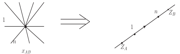
In more detail, the twistor actions consist of a holomorphic Chern-Simons action supplemented by a non-local term that generates the MHV vertex contributions. The axial gauge arises from a choice of a reference twistor denoted (or simply ) and is implemented by requiring that the component of any Dolbeault form should vanish in the direction of the lines through . In this gauge, the MHV vertices are the only vertices as the Chern-Simons cubic vertex vanishes. The propagator is the Green’s function for the anti-holomorphic Dolbeault operator () on twistor space. A key tool is a simple expression for this propagator that first appeared in this form in [14] but which built on calculations from space-time representatives appearing in appendix D (see also the last section of [2]). The propagator is essentially a superconformally invariant delta function which is a Dolbeault -form current that imposes the condition that , and should be collinear. The MHV vertices also have a description as products of the same superconformally invariant delta functions that enforce collinearity of the field insertion points.
Each NkMHV tree diagram yields an integral of a product of MHV vertices supported on lines and propagators with ends inserted on different lines. The propagators are delta-functions that restrict the insertion points on the MHV vertices to lie on a line through . The solution for the insertion points is unique and so the integrals over the insertion points can be performed explicitly against the delta functions in the propagator and vertices. We are left with the product of the MHV vertices but now with only external twistors inserted, multiplied by a certain standard superconformal invariant for each propagator. These are the twistor R-invariants of [34], but are now invariants of the standard superconformal group rather than the dual superconformal group. The R-invariants that arise are quite similar to those that arise in the momentum twistor version of the MHV formalism [11] (i.e., one for each propagator), but there are a number of differences: the R-invariants are those built out of ordinary twistors rather than momentum twistors, the geometry of the shifts for the boundary terms is different and in the momentum twistor formulation there are no vertex contributions.
We therefore obtain a straightforward calculus in which it is possible to perform the integrals arising for generic diagrams (both trees and loops). Here generic is meant in the sense of fixed NMHV degree and large particle number. In this generic case, we have at least two external particles on each vertex and the location of its corresponding line in twistor space is fixed by its external particles. The formulae make manifest the expected support of a given MHV diagram contribution in twistor space: NkMHV tree diagrams are supported on lines that correspond to the MHV vertices, connected by propagators. A propagator corresponds to the unique line that passes through the fixed ‘reference twistor’ and is transversal to the two lines corresponding to the MHV vertices at each end. Thus, as in the case of a BCFW decomposition, we obtain support on lines for a NkMHV tree amplitude, but here arranged as a tree with of the lines clearly playing a distinct role as propagators.
We obtain a similar support picture for loop diagrams with lines for each vertex and for each propagator. Remarkably, it is as easy to perform the integrals for a loop diagram as it is for a tree diagram, at least when the diagram is finite. For divergent diagrams, it is also possible to perform these integrals, but the results require regulation; there are many loop diagrams that do not lead to divergences though, and these can be evaluated as simply as tree diagrams in the generic case. These have the same structure as tree amplitudes, being a product of MHV vertices evaluated only on external twistors with R-invariants.
We will discuss a number of further ramifications of these ideas, including infrared divergencies and their possible regularisation, crossing symmetry, connections with momentum twistors and the Grassmannian formulation in §6.
The paper is structured as follows. After some brief preliminaries to establish notation and conventions, §2.2 reviews the twistor action for SYM and develops the theory of the superconformally invariant delta functions that provide the basic building blocks of the formalism. Section 3 then provides a derivation of the Feynman rules for this action in the CSW axial gauge. We obtain formulae for the propagator and for the MHV amplitudes (which are also the vertices in this formalism) on twistor space using the superconformal invariant delta functions developed earlier. §3.3 outlines the proof that these Feynman rules are equivalent to the momentum space MHV rules of [2]. Next, we demonstrate how the twistor space MHV formalism works at tree-level by giving explicit computations for the various classes of MHV tree diagrams in §4. We go on to show how this twistor formalism extends to loop diagrams. We consider the class of finite 1-loop non-planar MHV and planar NMHV diagrams, and the simplest case of the planar 1-loop MHV diagram in §5 and explain in general how to identify the divergences. Although we leave a full discussion of regulation of divergences to another paper, we dicuss this and a number of other key issues in §6.
The appendices contain discussions of the 2-point vertex on twistor space (A); the particulars of twistor theory for Euclidean signature space-time (B); the details of the proof deriving the momentum space MHV formalisms from that in twistor space (C); and the calculation of the twistor propagator from space-time representatives (D) which also demonstrates that the propagator we use is the Feynman propagator.
2 Background, notation and conventions
We adhere to the conventions of [35, 36] for bosonic twistors but twistor space will be super-twistor space, denoted , the Calabi-Yau supermanifold , with homogeneous coordinates:
| (2.1) |
where and are respectively negative and positive chirality Weyl spinors, and (for ) are anti-commuting Grassmann coordinates.
Points in complexified chiral super Minkowski space-time correspond to lines in twistor space by the incidence relation
| (2.2) |
These lines are Riemann spheres (s) and will be parametrized with the homogeneous coordinates .
The Penrose transform relates helicity solutions to the zero-rest-mass (z.r.m.) equations on a region in complexified Minkowski space to the first cohomology group of functions of homogeneity degree over the corresponding region in bosonic twistor space (); is the region swept out by lines corresponding to points of . We have
| (2.3) |
| (2.4) |
see for example [36] for a proof. Here denotes analytic cohomology. We will use the Dolbeault representation for the cohomology in which the cohomology classes are represented as -closed -forms modulo -exact ones. (See §6 for further discussion of other representations.) This transform is most easily realized by an integral formula
| (2.5) | ||||
| (2.6) |
where . The fact that these integral formulae yield solutions to the field equations can easily be seen by differentiating under the integral sign.
The standard choices of for positive/negative frequency fields are the sets
| (2.7) |
These are the sets that correspond in space-time to the future/past tubes , i.e., the sets on which the imaginary part of is past or future pointing time-like respectively. This follows from the fact that if we take and substitute into the incidence relation, then which has a definite sign when is timelike depending on whether is future or past pointing. The significance of this is that a field of positive frequency, whose Fourier transform of a field is supported on the future lightcone in momentum space, automatically extends over the future tube because is rapidly decreasing there, bounded by its values on the real slice.
Another frequently used set is on which ; this corresponds to excluding the lightcone of the ‘point at infinity’ in complex space-time.
2.1 The supersymmetric extension
The transform has a straightforward supersymmetrization to give an action for the superfield
| (2.8) |
where , , , , and are of weights , , , and respectively corresponding respectively to zero-rest mass fields .
The formulae (2.6) extend directly to this supersymmetric context to give superfields on space-times incorporating derivatives on (2.5)
| (2.9) | |||||
These fields have the interpretation as being the non-zero parts of the curvature
| (2.10) |
of the superconnection
| (2.11) |
Indeed, this superconnection can be obtained directly from via the Ward transform, which treats geometrically as a deformation of the operator on a line bundle and obtains as a (super)-conection on a corresponding line bundle on space-time.
2.2 The Twistor Yang-Mills Action
Here we give a brief review of the twistor action on for SYM [19, 20, 22] (these papers also discuss different amounts of supersymmetry, but we will stick to here).
The space-time version of this action is an extension to SYM of one introduced by Chalmers-Siegel for ordinary Yang-Mills. This action is a reformulation of the standard one designed in such a way as to expand around the anti-self-dual (ASD) sector. In addition to the connection 1-form on a bundle , they introduce an auxiliary SD 2-form , and action [37]:
| (2.12) |
where is the expansion parameter. Splitting the curvature into its SD and ASD parts, , this action gives the field equations
with the connection corresponding to . These equations are easily seen to be equivalent to the full Yang-Mills equations (), but for , they reduce to the ASD Yang-Mills equations with a background coupled SD field .
The full SYM action can be similarly written as a sum of two terms:
| (2.13) |
where accounts for the purely ASD sector and accounts for the remaining interactions which couple via the parameter , and are respectively the ASD and SD spinor parts of the multiplet and the scalars. Explicitly:
| (2.14) |
The Twistor Action
We now consider a topologically trivial vector bundle with -operator for . If the -operator is integrable, , the supersymmetric Ward transform [36, 38] gives a correspondence between such holomorphic vector bundles on twistor space and solutions to the anti-self-dual sector of SYM. The integrability conditions are the field equations of holomorphic Chern-Simons theory with action
| (2.15) |
Here depends holomorphically on the fermionic coordinates and has no components in the -directions. We can expand in terms of the to get
| (2.16) |
Since has weight 0 and has weight 1, we find that has weight 0, weight , weight , weight and weight . When taken to be cohomology classes, these give the multiplet appropriate to SYM under the Penrose transform with the lower case quantity on twistor space corresponding to its upper case counterpart on space-time.
To introduce the remaining interactions of the theory, we add the term
| (2.17) |
where is the line or corresponding to in and is a real 4-dimensional contour in the complexified Minkowski space ; is the restriction of the deformed complex structure to this ; and is the natural holomorphic volume form on chiral superspace:
Although might seem rather intimidating at first sight, we will see that it is easy to understand perturbatively and indeed this leads both to the finite set of terms in the space-time action in one gauge and the infinite set of MHV vertices in another. Although it is a section of a line bundle over , it can be checked that the integral of its log is independent of the choice of gauge as a consequence of the fermionic integration in this context [20].
Hence, the twistor action for SYM is:
| (2.18) |
This action has gauge freedom
| (2.19) |
and since has six real bosonic dimensions, has much more gauge freedom than the Yang-Mills action in space-time. In order to prove that (2.18) is equivalent to SYM on space-time, we must make a gauge choice which reduces (2.19) to the freedom of ordinary space-time gauge transformations. One particularly useful choice is a harmonic gauge up the fibres of a Euclidean fibration first introduced by Woodhouse [39] and this leads to the reduction to the space-time action as described in [20, 22].
3 The Twistor Space MHV Formalism
In [25], the MHV formalism on momentum space was recovered as the Feynman diagrams of the twistor action (2.18) in an axial gauge. This was done by using twistor cohomology classes that correspond to momentum eigenstates as the basic scattering states. Although this provides an explanation of the origin of the MHV formalism, it does not exploit the advantages that one might hope to gain from a twistorial formulation such as making contact with ideas from twistor-string theory and being able to exploit the superconformal invariance of the twistor formulation. The novelty of the following treatment is that the presentation will be self-contained in twistor space, using twistor cohomology classes that are supported at points of twistor space. This will bring out the underlying superconformal invariance up to the choices that are required to impose the gauge condition, and also make explicit the support of the various contributions to the amplitude.
We must first introduce the distributional wave functions that we will use as the asymptotic states for scattering processes: the elemental states supported at points of twistor space (these will in fact be the twistor transform of those originally introduced by Andrew Hodges [40]). These distributions turn out to be part of a framework of distributions supported at points, lines, planes and the bosonic ‘body’ in supertwistor space. These allow us to give a more careful treatment of the propagator and to better understand the MHV vertices.
3.1 Amplitudes, cohomology and distributional forms
As has already been mentioned, the asymptotic states for the particles in a scattering process are given by cohomology classes on twistor space in for . We will represent these as -forms that are -closed, , defined modulo the gauge freedom on some domain . Amplitudes are functionals of such asymptotic states. The kernel of an -particle amplitude will therefore be in the -fold product of the dual to such s. Although we could use the Hilbert space structure on such s, this turns out to be complicated in our context; we obtain the best formalism by representing the kernel of an amplitude using a local duality between -forms and distributional -forms that are compactly supported. This is simply given by
For manifest crossing symmetry, we must be able to take our asymptotic states to be of both positive and negative frequency, and so we must be able to take both or . This will be possible if the compact support of the amplitude is within . See below (3.16) for the example of the MHV amplitude.and §6 for further discussion.
Tree-level amplitudes in SYM can be decomposed in terms of color-sector subamplitudes; a -particle tree-amplitude can be written as:
where the sum runs over all non-cyclic permutations of the particles and the s are the generators of the gauge group. In this paper, we will be interested in the color-stripped amplitudes ; due to the color trace, these objects obey a cyclic symmetry in their arguments, and this will extend to the twistorial amplitude as a function of twistor wave functions or distributional forms. We make use of this cyclic symmetry both explicitly and implicitly often for the remainder of this work.
The amplitude will be defined modulo -exact forms with compact support as these will give zero by integration by parts. In an ideal world, an -particle amplitude would take values in . However, we will see that our amplitudes, including in particular the MHV amplitude fail to be -closed due to anomalies arising from infrared divergences, see (6.1) below. This failure of the amplitude to be -closed will lead to anomalies in gauge invariance. This is mitigated by the fact that throughout we will fix a gauge and, if we were to change the gauge fixing condition, quantum field theory would lead to very different formulae for the amplitudes. It is nevertheless a feature that should be understood better. See §6 for further discussion.
In order to obtain explicit formulae, we need to introduce some natural distributions on twistor space. We first note that on with coordinate , the delta function supported at the origin is naturally a -form which we denote
| (3.1) |
the second equality being a consequence of the standard Cauchy kernel for the -operator. This second representation makes clear the homogeneity property .
The fermionic delta function in the fermionic variable is
This follows from the Berezinian integration rule so that .
Following [34], to obtain delta functions on projective space we first introduce the Dolbeault delta functions on :
| (3.2) |
This is a -form on of weight zero. We then define projective delta functions by
These can easily be seen to be antisymmetric and to satisfy the obvious delta function relation
By integrating against further parameters, we can obtain the following superconformally invariant delta functions
| (3.3) | |||||
where cyclic permutations. The delta function will play a large role in what follows, giving both a representation of the propagator and being an ingredient of the MHV amplitude. It is antisymmetric in its arguments and has support where the three points , and are collinear and has simple poles where two of them coincide.
We can similarly define a coplanarity delta function
| (3.4) | |||||
Finally we can define the rational ‘R-invariant’
| (3.5) | |||||
where cyclic and . We will also abbreviate by . Although there are no longer bosonic delta functions, on the support of this fermionic delta function, the five twistors span a four dimensional space inside so that this can be thought of as a delta function supported on a choice of bosonic ‘body’ of supertwistor space. In the context of momentum twistors this is the standard dual superconformal invariant of [41]. The second formula is obtained by integration against the delta functions, see [34] for full details. This will also play a significant role in this story here, but as an invariant of the usual superconformal group as opposed to the dual superconformal group.
It will be useful to know how these delta functions behave under the -operator. In general we have relations of the form
where is ommitted. The right hand side necessarily vanishes for . We will have frequent use for the case of
| (3.6) |
so we give the derivation in full detail and leave the remaining relations as an exercise.
Since is a top degree form, it is -closed. Thus
where is the total -operator on the space of parameters together with the twistors , where is that on the s alone and being that on the s alone.
We can use this to calculate as follows
In the first equality we have taken under the integral, and in the second, we have used and used the fact that , in the third we have integrated by parts, and the fourth we have expanded out using finally to perform one of the -integrals to reduce it down to just one parameter.
We finally remark that with these distributional delta functions, many integrals can be performed essentially algebraically. Examples that we will frequently use are
| (3.7) |
3.2 The CSW Gauge and Twistor Space Feynman Rules
In order to obtain the dual form of the amplitude described above, instead of inserting wave functions into colour stripped amplitudes or vertices to obtain a number, we will insert external fields (for )
| (3.8) |
to obtain an expression for the amplitude taking values in the -fold tensor product of (one for each external particle).
To recover the MHV formalism on twistor space, we impose an axial gauge. The choice of reference spinor in the MHV formalism corresponds to the choice of a twistor ‘at infinity’ denoted ; this induces a foliation of by the lines that pass through . We require that should vanish when restricted to the leaves of this foliation:
| (3.9) |
This gauge explicitly breaks conformal invariance due to the choice of , but we will obtain a formalism that is invariant up to this choice. We will often refer to this as the CSW gauge as it was first introduced in [2].
The main benefit is that it reduces the number of components of from three to two, so the cubic Chern-Simons vertex in will vanish. Since this cubic vertex corresponds to the anti-MHV three-point amplitude, the choice of CSW gauge eliminates this vertex; anti-MHV amplitudes will of course still exist, but are now constructed from the remaining vertices of the theory. The twistor action becomes:
| (3.10) |
We now determine the Feynman rules of this action in twistor space.
Propagator
Usually the propagator is determined by the quadratic part of the action. However, there are two such contributions in (3.10): one from the kinetic Chern-Simons portion and another from the perturbative expansion of the (see (3.12) below). Since it occurs as part of a generating functional of vertices, we choose to treat this latter contribution perturbatively, so it will not enter into our definition of the propagator. However, this means that our formalism will include a two-point vertex. We discuss this issue in great detail later, and in appendix A, but the main point is that the two-point vertex itself vanishes as a conseqeuence of momentum conservation, and so never appears as a vertex in the diagram formalism. However, it does also play a role as a constituent of the higher point MHV vertices where it is no longer forced to vanish.
Hence, the propagator is fixed by the kinetic part of the action
to be the inverse of the -operator on acting on -forms in the CSW gauge (3.9):
The final answer is simply one of our superconformal delta functions
| (3.11) |
In order to check this, we need to see that it is indeed a Green’s function for and is also in the CSW gauge. The gauge condition follows from the fact that to obtain a non-trivial integral we must take the coefficient of in the expansion of the form part of and since this is accompanied by the constant , the remaining form indices are skew symmetrized with . To see that indeed defines a Green’s function, we have from (3.6) that, taking and as the reference twistor we have
The first term is the delta-function that we would like to have, whereas the last two terms essentially vanish in the degrees relevant to the inversion of the -operator on 1-forms; should be a -form in each variable, and , whereas the error terms arise from -components in and . Such minor ‘errors’ (or at least unphysical poles in momentum space) in the propagator are a familiar feature of axial gauges and are not problematic. Indeed, if we restrict ourselves to the open set in that excludes the ‘point at infinity’ (i.e., ), then the error terms do not have support and the Green’s function equation is satisfied exactly.
Vertices
In the CSW gauge the vertices all come from the logarithm of the determinant in (3.10) (the interactions of the full theory that we added to the ASD action). These vertices can be made explicit by perturbatively expanding out the logarithm of the determinant which gives [20, 25]
| (3.12) |
Here, is the restriction of the -operator from to , and is a field inserted a point . The are the Green’s functions for the -operator restricted to . If we suppose that the line is that joining twistors and , we can introduce the coordinate on by
| (3.13) |
In terms of this coordinate, is just integration against the Cauchy kernel
Thus, the th term in our expansion yields the vertex
| (3.14) |
Here the index is understood cyclically with and denotes a real slice of complexified space-time. In the action of course all the , but as a vertex in the Feynman rules, all the are allowed to be different. When the are the twistor wave functions that correspond to momentum eigenstates, we will see that this reduces to the standard -particle Parke-Taylor formula (3.24) for the MHV (recall that scattering amplitudes for incoming gluons in which gluons have positive helicity with the rest negative will be the NkMHV amplitudes in our conventions). amplitude [25]. This form, as an integral over the space of lines in twistor space, is a Dolbeault analogue of Nair’s original twistor formulation [42].
A key point in this formula is that the bosonic part of the integral is a contour integral in the space of complex , performed over the -dimensional real slice which can be taken to be some real slice of complex Minkowski space. The choice of signature of this slice will determine the support of the vertices that we obtain; if it is taken to be the standard Minkowski slice, our vertices will clearly be supported in as all the lines in the integration will lie in .
In order to obtain a manifestly conformally invariant formulation, we represent the volume form as
| (3.15) |
i.e., rather than represent the line as via (2.2) we use (3.13) and quotient by corresponding to the choice of and on .
Defining as in (3.8) will now give us the superconformally invariant formula
| (3.16) |
where we suppress color indices and the implicit trace. This form most fully manifests the symmetry of the amplitude, including the cyclic symmetry mentioned earlier. It is the twistor-string formulation [1, 15] given as a ‘path-integral’ over the space of lines. Having defined our external fields as -forms on , in (3.16), the integration over reduces the -form to a -form in each variable.
We can re-express higher point MHV vertices in terms of lower point ones multiplied by delta functions by the relation
| (3.17) |
To see this, observe that if we replace the variable by
then
Using this in the defining formula (3.16) for , we can separate out and an -integral
which leads to (3.17) as desired. This relationship between the point MHV amplitude and the -point amplitude appeared in a totally real version of (3.17) in [26] and has become known as an inverse soft limit [27].
This can be used to reduce the general MHV vertex to a product of delta functions and the two point vertex in many different ways. A typical such formula is
| (3.18) |
This formula exhibits explicit superconformal invariance and has a minimal number of residual integrations, but at the expense of the cyclic symmetry which is manifest in (3.16). We can obtain many such formulae for the MHV amplitude. The different versions are generated by the identity arising from the cyclic symmetry of the four point amplitude
| (3.19) |
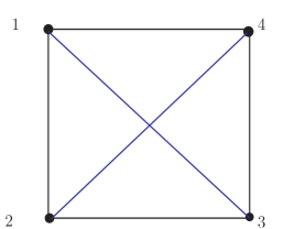
This can be understood pictorially via Figure 2, where (3.19) is the statement that the two triangulations of the square represented by blue lines are equivalent and that the location of is interchangable with that of any . For an MHV vertex with points, we can give a polygon representation of formula (3.18) in which the factors corresponds to a triangulation of the polygon using just the triangles (with their being one special line representing the residual two-point MHV amplitude). Then (3.19) allows us to change the given triangulation to an essentially an arbitrary triangulation leading to many alternate formulae for the MHV vertices. In general we will just use equation (3.17) and its cyclic permutations as necessary to pull out the dependence on twistors that need to be integrated and leave the remaining MHV vertices as residual factors in the answer.
In appendix A the two-point vertex is reduced to the integral
| (3.20) |
where the factors in the contour are now understood as arising from integrating and over the corresponding to and then integrating over the real slice of complexified Minkowski space (some other more concrete formulae are also given there but this will be sufficient for our purpose here). This is an integral of a -form over an -dimensional contour so that we are left with a -form in and (a -form in each factor). In particular if is the Minkowski real slice, and are pinned to lying on a line in and since the remaining collinearity delta functions in (3.18) force the remaining points to lie on this line, the general MHV vertex is supported for .
The 2-point vertex does not vanish, and indeed is a non-trivial factor in each of our vertices. Moreover it plays a nontrivial role in the calculation of correlation functions in the context of Wilson loops [14]. However, it is shown in appendix A that it is -exact in the sense of compactly supported cohomology, so if it appears on the exterior of a diagram, then it will give a vanishing contribution because it will be integrated against a -closed form. A more subtle argument should obtain when it appears in the interior of a diagram (see §3.3.1 and appendix A for discussion). Thus it never appears in the Feynman diagram calculus. In [25] it is shown that its evaluation on momentum eigenstates vanishes explicitly. However, because our amplitudes are cohomological they don’t need to vanish explicitly to be trivial in cohomology.
3.3 Derivation of Momentum Space MHV Formalism
As a reality check, we now show that the Feynman rules for the twistor action in the CSW axial gauge lead directly to the momentum space MHV formalism of [2]. This formalism was based on the use of the Parke-Taylor MHV amplitudes (3.24) below as vertices and scalar propagators, with the off-shell prescription for the vertices that the primed spinor associated to an off-shell momenta should be taken to be for some reference spinor (which as the notation suggests, is the Euclidean conjugate of the spinor part of the reference twistor).
In this complex framework, it is no longer possible to use the half-Fourier transform to convert the twistor amplitudes used here to momentum space. Nevertheless, it is possible to transform the ingredients of the MHV formalism on twistor space term by term into their counterparts on momentum space using (super) momentum eigenstates with supermomenta . For the propagator we will necessarily have , but the external particles will be on shell with
| (3.21) |
For such an on-shell momentum eigenstate we have the twistor cohomology class
| (3.22) |
That this gives the space-time momentum eigenstates can be verified directly for the component fields using (2.5) and (2.6); the integral is performed algebraically against the delta function enforcing (see [43] for a discussion of such individual momentum eigenstates).
To obtain the momentum space formula corresponding to a final integrated diagram on twistor space, we integrate out the form in each external twistor variable against the above Dolbeault -forms representing momentum eigenstates. However, we can go further and show that when expressed in momentum space, the vertices and propagators yield the appropriate CSW counterparts. We start with the vertices.
Momentum space representations break conformal invariance. So there is no loss in using a version of the MHV vertex in which the symmetry has been fixed by coordinatizing the line by the coordinate. This reduces the volume form on to , as in (2.2) yielding the formula
| (3.23) |
where as usual denotes the spinor inner product and we have ignored normalization factors. The first check is to show that these MHV vertices give the standard momentum space MHV amplitudes. This can be done by taking the to be momentum eigenstates as above (3.22). It is now easily seen that the delta functions allow the -integrals to be done directly, simply enforcing . The remaining integral of the product of exponential factors over now gives the super-momentum conserving delta function to end up with the Parke-Taylor [5, 6, 42] formula for the MHV tree amplitude extended to SYM:
| (3.24) |
where we have stripped off a normalization and an overall color trace factor, and the supermomentum conserving delta-function is
with
These Parke-Taylor MHV amplitudes (3.24) are the vertices in the momentum space MHV formalism extended off-shell by associating the primed spinor to an off-shell momentum . To see how this arises from our twistor space formalism, we first remark that the integrals in (3.23) are over (a contour in) the spin bunde coordinatized by where is real. This has a natural projection to twistor space following from (2.2) given by:
The MHV vertex is evaluated by first pulling back the cohomology classes for the external fields and for the propagators to the spin bundle , and then integrating using (3.23). In order to obtain a momentum space representative, we wish to Fourier transform the ingredients so as to replace the integral by a corresponding momentum space integral; this is a conventional Fourier transform over a real slice. We pull back to using and Fourier transform in the and variables to obtain the Fourier representation
| (3.25) |
After some calculation we obtain
| (3.26) |
where is related to the original constant spinor (the primary part of ) by means of a quaternionic complex conjugation induced by the choice of Euclidean real slice (see appendix B). Appendix C contains the details of these calculations; in order to obtain the correct answer here, it was necessary to perform the Fourier transform on a Euclidean real slice.
If we now substitute this expression for the propagator into the MHV vertex (3.23), then the delta functions in and again allow these integrals to be done algebraically with the effect of substituting them with the primed spinor . The integral over then incorporates the supermomentum into the supermomentum conserving delta function. This corresponds exactly with the prescription given by [2] for the momentum space MHV formalism as required.
3.3.1 The vanishing of the 2-point vertex
It is now straightforward to show, via this transform to momentum space, that the two point vertex does not play a role in the formalism: if it is present in a diagram, the whole diagram will vanish. The most nontrivial case is when the vertex is in the middle of the diagram with propagators attached to each leg with supermomenta and . The fermionic part of the momentum conserving delta function in (3.24) then reduces to and so the spinor products cancel those in the denominator, yielding an overall in the numerator. The bosonic delta function then forces so that , and the numerator factor then forces the vertex to vanish.
4 Tree Diagrams
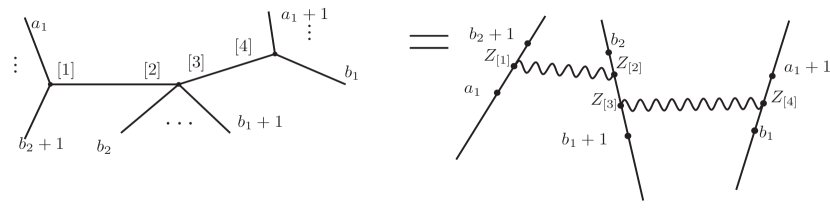
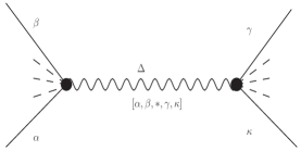
Having demonstrated that the twistor action in CSW gauge produces a perturbative expansion equivalent to the momentum space MHV formalism, we now endeavour to calculate amplitudes in a manner which is self-contained on twistor space. The Feynman rules using the propagator and vertices we have just obtained lead to formulae for amplitudes in terms of integrals over intermediate twistors in the standard way. We will see that for generic diagrams all these integrals can be performed explicitly. We will find that each NkMHV diagram yields a product of MHV amplitudes/vertices multiplied by R-invariants. The MHV vertices are those corresponding to the external legs of each of the vertices and there is an R-invariant for each propagator; the R-invariant has five arguments, one of which is always the reference twistor and the other four are the external twistors adjacent to the propagator when propagators are not inserted adjacent to each other at a vertex. Such a picture holds when no propagators are adjacent at a vertex and we will refer to these as generic diagrams (which is the case for fixed and large , but will not be the case when approaches ). When propagators are adjacent we call the diagram a boundary term and either the nearest external twistor, or a shifted version thereof is used to determine the R-invariant. There are also boundary-boundary terms in which some vertex has fewer than two external vertices. Here there are not sufficient delta-functions to integrate out all the internal twistors and some integrals remain.
4.1 Tree-level NMHV Amplitudes
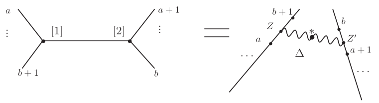
A tree-level NMHV amplitude is expressed in the MHV formalism by a sum over tree diagrams, each with two MHV vertices joined by a single propagator. The corresponding picture in twistor space, given in Figure 3, has a line corresponding to each of the two MHV vertices of (3.18) connected by a propagator as given by (3.11). Thus, the contribution of such a term to the NMHV amplitude is:
We can simplify this using (3.17) to obtain
The first two factors here are MHV amplitudes. The remaining factor can be integrated explicitly against the delta functions using (3.3) as follows
Hence, we see that such a contribution to the NMHV amplitude is given by:
The sum over tree diagrams gives the NMHV amplitude as
| (4.1) |
We remark that the corresponding formula in momentum twistor space is , which is the formula above stripped of the MHV factors.
4.2 Tree-level MHV Amplitudes
At MHV, there is still essentially one family of diagrams, Figure 4, with the external legs distributed around it in all possible ways. However, our treatment will be different in the two cases either where the two propagators are not or are adjacent (i.e., not separated by external particles) Figure 4 or 5 respectively. We refer to these as ‘generic’ and ‘boundary’ diagrams. The twistor space support of these diagrams is also shown in Figures 4 and 5.
Generic terms
Applying our twistor space Feynman rules for the MHV formalism, a diagram of this sort gives:
| (4.2) |
We can use (3.17) four times (twice on the middle vertex and once each on the others) to replace an MHV vertex by one with one fewer arguments multiplied by a to isolate the dependence on the propagator variables to get
These integrations can be done against the delta functions just as in the NMHV case to obtain R-invariants. This gives an R-invariant for each propagator multiplied by an MHV amplitude for each vertex to yield
| (4.3) |
for the general contribution to the N2MHV amplitude with non-consecutive propagators.
Hence, after the integral over propagator insertions has been performed, the remaining external legs on the middle line of Figure 4 can be treated as a single MHV vertex, with the propagator insertions removed.
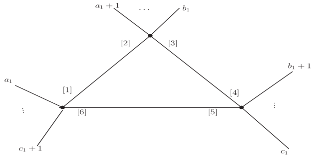
Boundary terms
A boundary diagram, on the other hand, is one in which the propagator insertions are adjacent on the middle vertex (see Figure 5). We obtain
| (4.4) |
As before we can use (3.17) to factor out three MHV amplitudes/vertices, one for each vertex, depending only on the external twistors. Because of the adjacency of and on the middle vertex there are two ways to do this depending on which of these propagator insertions we use (3.17) on first. Taking first we obtain
| (4.5) |
proceeding to do the and integrals as before, we obtain
Here we see that is inserted into the first R-invariant but will be fixed by integration against the remaining delta-functions. It is clear that is uniquely determined to be at the intersection between the line joining to and the plane spanned by . We therefore define
which will be the final value of . Now, integrating out and against the delta functions we obtain
| (4.6) |
If we had decomposed the middle MHV vertex using (3.17) in a different order, removing first and then , we would have obtained a different, albeit equivalent, formula. Following the above procedure, we obtain
| (4.7) |
where
As in the momentum twistor case, these two shifts are equivalent in the sense that (4.6) and (4.7) are equal.
Boundary-Boundary terms
There is a final class of N2MHV diagrams that doesn’t quite fit into the above framework; those in which there is only one external particle on the middle vertex (see the first diagram of Figure 9. This yields
and by pulling out a delta function from the middle vertex reducing it to a two-vertex, we can integrate out to reduce to
| (4.8) |
At this point the remaining intergrations can be performed in various ways, for example one can use the remaining explicit delta function or one of those implicit in the 2-point vertex to perform (some of) the remaining integration. (If one were working in Euclidean signature, we could use (A.9) to obtain a formula as a product of R-invariants but involving a complex conjugate twistor.) However, the integral over the space of lines through the given fixed point on the middle vertex is essential. If these lines are to correspond to points of real Minkowski space, then this is a one-dimensional integral, but in Euclidean signature this would be zero-dimensional.
4.3 MHV Tree Amplitudes
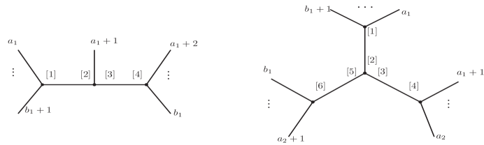
We now extend this computational strategy to general MHV tree amplitudes. For arbitrary , the amplitude is built from a sum of diagrams, the building blocks of which we have already encountered at the MHV level: generic terms (i.e., diagrams with no adjacent propagator insertions); boundary terms (i.e., diagrams in which one or more vertices have two or more adjacent propagator insertions); and boundary-boundary terms (i.e., boundary terms in which a vertex with adjacent propagator insertions has fewer than two external legs). We deal with each type of term separately in what follows.
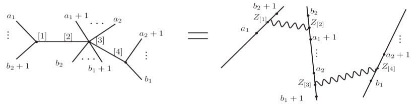
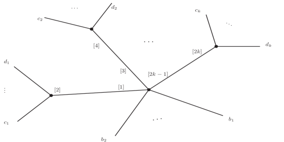
4.3.1 Generic Terms
For diagrams in which there are no adjacent propagator insertions at any vertex, our twistor space Feynman rules generalize directy from our prior investigations. At each vertex, using (3.17), we can strip off a at each propagator insertion leaving an MHV vertex that depends only on the external particles at that vertex. Each propagator is then multiplied by the and that have been stripped off from the MHV vertices at each end. Here and are the two nearest external particles on one side of the progagator, while and are the closest on the other side (see Figure 6). As before, the integrations over and can be done algebraically against the delta functions to yield the -invariant .
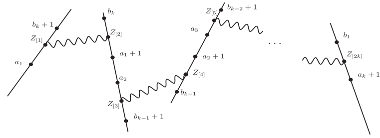
As an example, consider the generic term with diagram in twistor space given by Figure 7. Stripping off all external MHV amplitudes and then integrating over propagator insertions gives, in the numbering scheme for the external particles used by the diagram:
Of course, for generic non-boundary tree diagrams, the precise form of the contribution to the overall amplitude will depend on the diagram’s topology. However, the formula is constructed algorithmically as described above with MHV amplitudes built from external particles at each vertex, and R-invariants built by connecting the external particles closest to the two ends of each propagator and the reference twistor.
4.3.2 Boundary Terms
A boundary term will be a diagram for which some propagators are inserted next to each other on some vertices, although we will for the time being require that there are at least two external particles on each vertex.
For boundary terms, the formulae are similar to the non-boundary case: we obtain a product of MHV amplitudes, one for each vertex containing only the twistors for the external particles at that vertex, and R-invariants, one for each propagator. However, because of adjacent propagator insertions, some of the entries in the R-invariants associated to the propagators are now shifted.
The rule for the shifts can be obtained by studying each end of the propagator separately; the R-invariant for a given propagator will still have two pairs of twistors inserted into it, each pair lying on one of the two lines associated to the vertices into which the ends of the propagator are inserted.
To give the most general case, we compute the shifts at a vertex with adjacent propagators as in Figure 8. We now use (3.17) to decompose the central vertex into a product
It is clear that we have made a choice in doing this and we could easily have chosen the opposite orientation or indeed made other choices. The factor of will be left as part of our final answer, but we will seek to use the delta functions to integrate out the . Introducing the propagators, the relevant integrals for the are
| (4.9) |
where . These can be done inductively starting from and decreasing using the fact that we know that the lie on the lines . Performing the integral against the delta functions yields . Given that is fixed to lie on the line , must be fixed to lie, not only on but also on the plane through and . Thus we can substitute
| (4.10) |
into the remaining formulae. Now that is fixed we can carry on and integrate and so on by induction. We finally obtain for the integral (4.9)
| (4.11) |
where now the are fixed twistors defined by
| (4.12) |
To obtain a product of R-invariants we must now integrate out the against the obtained from (3.17) applied to the vertex on which it lies. Assuming no adjacent propagators to these on those vertices we obtain, as before, for the diagram in Figure 8 the contribution
We have done this calculation for the case where just one end of a propagator is adjacent to another, but we can state the rules for a general diagram as follows:
-
•
Each vertex in the diagram gives rise to a factor of an MHV vertex in the answer that depends only on the external legs at that vertex.
-
•
Each propagator corresponds to an R-invariant where and are the nearest external twistors with in the cyclic ordering on the vertex at one end of the propagator, and similarly for on the vertex at the other end. Let be the insertion point on the vertex containing and . We have that is shifted according to the rule
(4.13) The rule for follows by .
4.3.3 Boundary-Boundary Terms
We now turn to the boundary-boundary contributions when there are fewer than two external legs on some vertices where the above prescription breaks down: there will be no line to use in the definition of the shifted s so the shifts prescribed by (4.13) for the boundary terms cannot be defined. See Figure 9 for simple examples of such diagrams; we already considered the first of these in our discussion of the N2MHV case. In that case there remained one external leg on the diagram, and we were left with an integral over one remaining internal twistor in (4.8), although in principle, this can be reduced to an integral over the space of real lines through the given fixed twistor which in Minkowski signature is one-dimensional, and in Euclidean signature, zero-dimensional. In general it can be worse than this: we can have vertices with no external legs and our procedure will leave us with two remaining twistors to integrate out. The simplest of these is the second diagram in Figure 9 and we work through this.
The N3MHV ‘cartwheel’ diagram represents essentially the worst-case scenario for a boundary-boundary term. It gives rise to the integral
where is the 2-point MHV amplitude given by (3.20).
We emphasize that although we have not been able to reduce boundary-boundary terms to a simple expression in terms of shifted twistors, they are still fully described by the twistorial MHV formalism. It is possible to reduce these further using the remaining delta functions, but there is no reason in the case where there are no external legs on a vertex not to be integrating over the full real four-dimensional space of real lines. It seems to be impossible to obtain an expression built only out of R-invariants and MHV vertices. However, we again stress that with a choice of real contour these remaining integral could be performed (and do not introduce divergences); this would simply entail the introduction of new signature-dependent machinery which we choose to avoid here.
A full NkMHV tree amplitude is then computed in the MHV formalism on twistor space by summing the contributions for all non-boundary, boundary, and boundary-boundary terms for the given specification of external particles and MHV degree.
5 Loop diagrams in Twistor Space
We know that loops are calculated correctly from the MHV formalism in momentum space at least at 1-loop [10] and as far as the loop integrand in the planar part of the theory is concerned it has been shown to be correct to all loops for four-dimensional cut-constructable theories [12]. The status of the MHV formalism at one loop and beyond in non-supersymmetric gauge theories is still speculative, because MHV rules miss the rational contributions to a scattering amplitude. Furthermore, these loop amplitudes are generically divergent in four dimensions and require regularization. We give here only a very superficial analysis and consider only the simplest finite diagrams. We consider also some of the diagrams of the MHV 1-loop amplitude but our analysis here will be inconclusive. In particular, we will not regularize or introduce the Feynman prescription (but see §6 for some discussion of this).
5.1 Finite examples
In order to start with finite examples, we consider first a non-planar diagram at MHV and secondly a planar diagram at NMHV to show the simplicity of the extension of the above ideas to loop amplitudes.
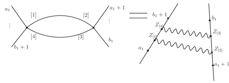
5.1.1 Non-planar 1-loop MHV diagrams
For 1-loop diagrams at MHV we have two vertices connected by two propagators. In the planar case the propagator must be adjacent to each other on both vertices as in figure 12 and we will see that these are divergent. In general the propagators can have arbitrary separation and we consider these separated cases first as shown in Figure 10. Such diagrams are non-planar.
It is straightforward to see that we can integrate out the intermediate twistors against delta functions obtained from the vertices by (3.17) exactly as at tree-level and indeed the resulting expression:
| (5.1) |
follows from the rules that we gave for generic tree diagrams. (We give more details in the calculation for the divergent planar case below). However, the geometry underlying this calculation is instructive. The twistors that were integrated out to obtain this formula were constrained to lie on the lines associated to the vertices. The propagators also fixed these points so that they lie on the (unique) line through that is transversal to the lines associated to the MHV vertices. Thus the insertion points of the two propagators at a given MHV vertex end up being the same points. The MHV vertex has no singularity when points come together unless they are adjacent in the colour ordering where they have a pole. Here in this generic non-boundary case they are not adjacent. In the boundary case one anticipates therefore one degree of divergence as two ends of the propagators must lie on top of a pole. In the planar case we will see a double divergence as both ends of the propagators will be adjacent.
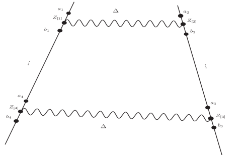
5.1.2 Planar NMHV at 1-loop
Two types of diagram contribute to the NMHV amplitude at 1-loop, one divergent and one finite. The finite cases are as in Figure 11 (the divergent ones are the same as the MHV case with an additional vertex connected by a propagator into one of the vertices).
The computation of the the internal integrals follows identically to the tree-level cases above. Using the numbering scheme for external particles indicated by Figure 11, we can trivially integrate over , and to give:
The remaining integrals can be performed against the delta functions yielding the shifted twistors for , , respectively, as before to give:
where
5.2 Planar 1-loop MHV
The diagrams for the planar 1-loop MHV amplitudes all have the same form as given by Figure 12 (although we do have boundary terms when there is only one leg on one of the vertices).
In the generic case, we have enough delta functions to integrate out the as in the tree-level cases above. However, the geometry of the relations implied by the delta functions (as in the non-planar MHV case) forces the point to be coincident with and to be coincident with . This is because the propagators force both the pairs and to lie on the common transversal to the two lines through as indicated in Figure 12). Given two lines in general position (i.e., those corresponding to the two MHV vertices) and a point in not on those lines (here the CSW reference twistor ), there is a unique transversal connecting the lines and intersecting this point. Hence, the lines and must in fact be the same, which in turn means that and . Now, the MHV vertices have simple poles whenever any two of their arguments coincide, so the geometry evaluates the two vertices at one of each of their poles.
Using the reduced rules above obtained by naively performing the integrals against the delta functions gives
where
Considered on its own, each R-invariant can be seen to contain a divergence arising from the geometry outlined above. Indeed, recall that
and observe that from its definition, is co-planar with , , and and hence the denominator factor of . There is a similar zero in the denominator of , so we obtain a ‘’ from each R-invariant. However, considered together the fermionic parts of the two R-invariants are proportional to each other and so using the nilpotency of these expressions, these numerator terms vanish 111We thank Mat Bullimore for this observation
Clearly, the divergence (or non-divergence) properties of this planar 1-loop MHV amplitude are dependent upon a careful treatment of this ‘0/0’. Presumably careful regularization should only be required for those of these diagrams that are actually divergent, and taking care of the Fermionic structure first before performing the integrals should lead to finite answers for the generic finite case of these diagrams. Genuine divergences only arise in the case when one of the vertices is the 4 point vertex [28]. To make sense of the genuinely divergent cases, regularization is required and we discuss this further in §6.
There does not seem to be a correlation between boundary-boundary terms and divergences as one might have initially feared (although of course that is not to say that there are not divergent boundary-boundary diagrams).
6 Discussion and further directions
We have seen that it is possible to formulate scattering amplitudes in twistor space in such a way as to deal with both their cohomological and invariance properties explicitly if we regard amplitudes as being in the ‘topological dual’ to the wave functions; that is, as tensor products of s with compact support rather than as s where the wave functions live.
Using this approach we were able to take the twistor action in the simplest axial gauge, the CSW gauge, and obtain its Feynman diagrams. At tree level we discovered that for a large class of diagrams, as in momentum space, one can perform the internal integrals against delta functions to give an expression as a product of MHV vertices, one for each vertex in the diagram but evaluated only on its external particles, and an R-invariant for each propagator. This is not quite possible when a line for the vertex is not determined by external particles on that vertex, which is the case when there are fewer than two external legs attached. However, in contradistinction to momentum space Feynman rules, this integration against delta functions is still possible for loop diagrams although one then sees the divergence directly, and we have not yet introduced a suitable regulation. This is a major problem that we have not begun to address here.
Cohomology, crossing symmetry and anomalies
As has already been mentioned, wave functions on twistor space are cohomology classes in , being -forms that are -closed () defined modulo the gauge freedom on a domain . Amplitudes are functionals of such wave functions representing the asymptotic states that are to be scattered. Crossing symmetry tells us that it shouldn’t matter whether the wave function is incoming or outgoing (i.e., positive or negative frequency). The positive/negative frequency condition is the condition on the set being .
In the first instance therefore, the kernel of the amplitude is in the -fold product of the dual to such s. Since the external wave functions are elements of a Hilbert space, one usually imagines that one can blur this distinction between the space of wave functions and its dual as the Hilbert space is dual to itself. However, for twistor theory in Lorentz signature, this duality is somewhat involved: the first step in defining the Hilbert space structure on a wave function is complex conjugation. This maps twistor space to dual twistor space. The Hilbert space structure therefore requires the use of the ‘twistor transform’ from cohomology classes on dual twistor space to map them back to twistor space to a class with weight on where it is dual to the original class in by integration over . Thus, the duality is highly non-trivial and there is a big difference between dual descriptions. Unitarity is not manifest on twistor space.
Rather than use the nonlocal Hilbert space structure, we have represented the kernel of an amplitude using the local duality between and where the subscript denotes compact support. Crossing symmetry is then made manifest when this compact support lies in so that it makes sense when integrated against external fields of both positive and negative frequency. This support was made clear in the definition of the vertices in which the external twistors were all required to lie on a line that corresponds to a point of real Minkowski space. Such lines automatically lie in .
Thus, our amplitudes took values in the -fold tensor product of
To obtain a functional of wave functions, we use the natural duality between - and -forms on given by:
It is defined modulo of forms with compact support as these will give zero by integration by parts. To obtain a formula for the amplitude as a functional of wave functions of external particles, we simply pair the amplitude with the external wavefunctions to obtain the normal amplitude. See (3.16) above for the example of the MHV amplitude and (A.6) where we show that the 2-point vertex is exact so that it vanishes as an amplitude.
The amplitude ought to be -closed with compact support for the integral to only depend on the cohomology class of . If so, we would have that the amplitude take values in the cohomology groups . However, in our context, we have gauge-fixed and so this is not an absolute requirement and indeed these groups vanish. The MHV amplitude itself seems reasonably canonical, and so one might hope that it at least is -closed. We find by direct computation along the lines of that leading to (3.6)
| (6.1) |
This is a clear obstruction to realizing the amplitudes as cohomology, and indeed this equation expresses the standard infrared singular behaviour of amplitudes under collinear limits. One can understand this equation as implying that, when understood as an , the amplitude has a simple pole on the diagonals. See [44] for a discussion of how such objects can be understood in algebraic geometry.
Thus, the failure of the amplitude to be -closed would seem to be an anomaly arising from infra-red divergences. It leads to a failure of gauge invariance, but the machinery of quantum field theory has in any case required that we fix our gauge. A different gauge fixing would lead to very different formulae for the amplitudes. The anomalies are associated to the same poles in the MHV amplitude that gives rise to anomalies in (super-)conformal invariance as noted by [45] and it seems likely that a proper coholomogical treatment will require a similar treatment to that given there.
Comparison to the momentum twistor formulation
It is instructive to compare the twistor space version of the MHV formalism to that in momentum twistor space. Momentum twistors were introduced by Andrew Hodges [13] and are based on dual conformal invariance. The dual conformal group is the conformal group acting on region momentum space, an affine version of momentum space. It arises from T-duality in the AdS/CFT correspondence [46], but had already been observed in the integrands of certain loop amplitudes [47] and was seen to extend to all planar amplitudes in various works [48, 41, 49, 50, 51, 52]. The transform from momentum space to momentum twistor space is essentially a local coordinate transformation that uses the twistors for the dual conformal group rather than the standard conformal group and makes manifest that invariance. The MHV formalism was reformulated in momentum twistor space in [11] (and this was the framework in which the proof of the all-loop integrand for the planar MHV formalism was obtained [12] by extending the recursion methods of [7, 8, 9]).
The correspondence between the two different twistor space MHV formalisms is relatively simple, but with important differences. This is despite the fact that momentum twistors and ordinary twistors are related in a highly non-local way (in split signature by the half-Fourier transform) reflecting T-duality on space-time. In momentum twistor space, the vertices of the MHV formalism simply correspond to 1, and the propagators are given by the R-invariants, now for the dual superconformal group. If we compare this to the MHV formalism in twistor space obtained in this paper, in generic diagrams we obtain precisely the same R-invariants for the propagators, except here they are functions of twistors, whereas in the momentum twistor version they are functions of momentum twistors. However, in twistor space the MHV vertices are not 1, but are given by the standard twistor MHV formula, i.e., as the product of delta-functions that ensure collinearity. However, for the boundary diagrams, although shifted twistors need to be used in both versions of the formalism, the geometry of these shifts are different in the two different twistor versions of the formalism.
At the level of the action, the twistor action was also used to obtain the momentum twistor version of the MHV diagram formalism [14]. However, in this context it was obtained as a diagrammatic expansion for the correlation function of a (holomorphic) Wilson loop in twistor space rather than an amplitude. (This gave the first proof of the Wilson-loop amplitude correspondence and indeed the first formulation that extends beyond MHV amplitudes [53]; it also leads to a definition of a supersymmetric space-time Wilson loop.) However, it is worth remarking that in this context the Feynman diagrams for the correlation functions are the planar duals of those for the amplitudes. That these can lead to the same formulae is only possible because, for momentum twistors, the vertices are just given by 1.
Other axial gauges
It is worth noting that the CSW gauge is by no means the only axial gauge. One only needs to choose a holomorphic 1-dimensional distribution and require that . The simplest way to do this is to choose a global holomorphic vector field (so that is the span of ) and require that . The CSW gauge arises when corresponds to a null translation, but we can in principle adapt to any problem we choose.
The vertices do not change if we change the gauge, but the propagator does. For example, if , as arises from a timelike translation, we obtain for the propagator
| (6.2) |
where . It is conceivable that such a propagator will give rise to alternative useful formulae.
Feynman prescription
A final issue that we have not explicitly spelt out is how to ensure that we have incorporated the Feynman prescription into the propagator. An automatic way of doing this is to analytically continue to Euclidean signature; this is implicit in our form of the propagator. Indeed, we see in appendices §B–D that in order to obtain the momentum space propagator correctly, it is necessary to perform the calculation on the Euclidean real slice. However, this also implies that in the definition of the two-point vertex, the ‘real’ contour of Minkowski space must be understood to include an ‘ shift’ of the Lorentzian real slice (i.e., one that is topologically equivalent to the Euclidean slice). This must be understood in a limiting sense if we also wish to maintain manifest crossing symmetry which requires us to take the limit back onto the Lorentzian real slice.
6.1 Open questions
Tree amplitudes
It would be helpful to have some further analysis of the boundary-boundary terms. We have not pushed them further here as they do not fit into our generic pattern of reducing to MHV vertices with just external particles multiplied by an R-invariant for each propagator. Furthermore, these diagrams do not have a special status in momentum space (or in momentum twistor space). There are nevertheless further delta functions within the two-point vertex that we haven’t exploited. In the case of a vertex with no remaining external legs, we will be left with a four dimensional integral that is unconstrained by delta functions. With just one external particle, in Lorentz signature, there is one remaining integral, whereas in Euclidean signature there are none.
One unsatisfactory feature of our discussion is our treatment of the two-point vertex. We know that it does not contribute from momentum space arguments, as shown in §3.3.1, and it is also easily seen to vanish from the point of view of the twistor action by evaluating it on off-shell momentum eigenstates—this was the argument used in [25]. However, it is not so obvious why it vanishes within the formalism used in this paper (see Appendix A for some further formulae and discussion). The puzzle is sharpened by the fact that the 2-point vertex does not vanish when evaluating correlation functions; in the context of the holomorphic Wilson loop in twistor space [14], it is the basic ingredient in the MHV 1-loop amplitude.
Loop amplitudes
It is striking that for many loop diagrams, it is possible to perform all the integrals against the delta functions and that their evaluation is essentially as easy as at tree-level. This is clearly quite different from the momentum space (or indeed momentum twistor) framework in which there are always four remaining integrals at each loop order. This leads to the possibility that this could become a more efficient formalism than that in momentum space. However, we need to have a systematic scheme to cope with divergences to make it useful. The usual strategy on momentum space is to regularize divergences using dimensional regularization (c.f., [10]). This would seem to be awkward to apply in a twistorial context as twistor-theory does not scale so easily to higher dimensions. An easier approach is to use the mass regulation using the Higgs branch introduced in the context of the AdS/CFT approach to scattering theory in terms of string theory on [54]. In the context of momentum twistors this leads to local adjustments to the formulae on momentum twistor space which arise from the same twistor action, and so could lead to a scheme that is applicable in our context. Ideally we would regulate the whole theory in this way and obtain regularized amplitudes as an output. It remains to be seen whether such a regulated theory would be as computable as that described above.
Another approach to regulation is to simply focus on finite terms. It is a standard fact that divergences are controlled by those at 1-loop (or indeed from the Wilson loop point of view, from the theory) and the cusp anomalous dimension. Thus one can cancel divergences and focus on the finite remainder. A particularly elegant strategy here would be to directly calculate the finite cross-ratio expressions used in the OPE approach of [55].
An important feature of loop amplitudes is the relationship between the transcendentality degree of functions (polylogs) of momenta and the loop order (i.e., at -loops, the functions and coefficients have transcendentality degree and -logs appear), see [56, 57] for applications. Since there is, at least in a moral sense, a half-Fourier transform between our relatively accessible expressions and those on momentum space we shouldn’t be expecting to see polylogs directly. Nevertheless, one might hope that there should be a direct way of recognising the symbols of the polylogs that arise. As a first step, one should perhaps already be able to see the transcendental coefficients of the cusp anomalous dimension as one attempts to cancel divergences in multi-loop diagrams with those in powers of the 1-loop amplitude according to the definition of the finite parts of the log of the amplitude that arises in the Wilson-loop point of view. Perhaps more importantly, we should be able to simply use the transform to momentum space described above (3.22) to obtain the polylogs directly from the fully integrated loop twistor MHV diagrams.
The Grassmannian connection
In the Grassmannian construction of [58, 34, 32], tree amplitudes and the leading singularities of loop amplitudes at NkMHV are obtained as residues of a contour integral involving superconformally invariant delta functions of the form used in this paper over the Grassmannian of -planes in in . In [59] the connection with the MHV formalism in momentum twistor space was established at NMHV using a recursion argument. By incorporating this work (and that in [11] for momentum twistors) we should be able to obtain a more systematic formulation of the full amplitude in the Grassmannian derived from Lagrangian principles. A particular advantage of the Grassmannian formulation is that global residue theorems can be used to obtain equivalences between different formulae for the same amplitude and allow us to obtain improved formulae. In particular, it would be a great help in the regularisation problem to obtain twistor (as opposed to momentum twistor) forms of the ‘local’ versions of the loop amplitude integrands found in [60].
Acknowledgments
We are grateful to Fernando Alday, Nima Arkani-Hamed, Freddy Cachazo, and Andrew Hodges for useful and stimulating conversations and particularly David Skinner and Mat Bullimore for a number of ideas and contributions that may not be fully acknowledged in the text. We further thank Gabriele Travaglini and Ed Witten for raising issues that led to the correction of erroneous claims in earlier versions of this article. TA is supported by the NSF Graduate Research Fellowship (USA) and Balliol College; LM is supported by the EPSRC grant number EP/F016654.
Appendix
Appendix A The 2-Point vertex in twistor space
We showed in §3.3.1 that the two point vertex vanishes, but we have not been able to see this directly in twistor space. In this appendix we give a number of twistor space formulae for the 2-point vertex showing in particular that it is -exact so that it plays no role in the Feynman diagram formalism when inserted onto an external leg. Recall that the 2-point vertex on twistor space is given by the expression
| (A.1) |
This can be reduced in a number of ways. Firstly note that the fermionic part of the integral can be performed directly algebraically against the fermionic delta functions to yield a factor of leaving an object with no fermionic dependence
| (A.2) |
Here we define
where the subscripts denote the homogeneity in the first and second entry respectively. The can be taken out by fixing , and reducing the and integrals to projective integrals. Removing the appropriate Jacobian factor we obtain
| (A.3) |
where the factors in the contour are now understood as arising from integrating and over the corresponding to and then integrating over the real slice . This is an integral of a -form over an -dimensional contour so that we are left with a -form in and (a -form in each factor).
It is possible to reduce this further, but it is at this point possible to express this as an exact form using a bosonic version of (3.6). Define
| (A.4) |
Then as in (3.6) we have
| (A.5) |
(There is no term as there is no pole in in (A.4).) Thus we can write
| (A.6) |
as on the support of the term. Thus is an exact form.
We now present another pair of formulae for the two point vertex. Breaking manifest conformal invariance we can write:
| (A.7) |
We can maintain conformal invariance, if we are are prepared to use a Euclidean real slice for and this representation could well be useful for Euclidean signature correlation function calculations (although less appropriate to the S-matrix computations of this paper). In this case one of the bundles over can be taken to be the whole of the twistor space parametrized by and we can then integrate out the delta function in (A.3) to obtain
| (A.8) |
The remaining integral is that over the real in twistor space that contains . For a Euclidean signature real slice we must have for the bosonic part where is the Euclidean conjugate. We can now integrate over the complex -plane to obtain
| (A.9) |
This is the bosonic collinear delta function
| (A.10) |
where the subscripts denote the weights in its arguments.
Although our statement of -exactness for the two point vertex ensures that it does not contribute to the Feynman diagram formalism when inserted onto an external particle leg in any diagram (using integration by parts and the fact that it is paired with an on-shell external wave-function), it is not so obvious that its contribution vanishes when it is inserted on an internal (i.e., propagator) leg. This is because an integration by parts argument moves the -operator onto a propagator (which is not -closed) rather than a cohomology class. Explicitly calculating the contribution in this case yields an integrand which is exactly the same as that arising in the computation of the so-called ‘Kermit’ diagrams in the momentum twistor version of the MHV formalism [11]. This contribution plays a crucial (non-vanishing) role in the momentum twistor framework (essentially computing the 1-loop MHV contribution) and certainly does not vanish as an integrand. However, our formalism is a term-by term transcription of the momentum space MHV formalism to twistor space, and the two point contribution does not contribute on momentum space. Furthermore, as we have mentioned, using the Euclidean space formalism of [25, 22] we can evaluate the two-point vertex on off-shell momentum eigenstates and see directly that it vanishes.
This tension between the picture on twistor space presented here (where the two point contribution must vanish) and the momentum twistor formalism (where it must not) is clearly a subtle issue that requires further attention. As we have mentioned, the two calculations are identical at the level of the integrand they produce, the crucial difference manifests itself in the choice of real contour.
Appendix B Twistor space and Euclidean space-time signature
The main exposition of this paper has focused on aspects of the twistor space MHV formalism which are independent of the choice of space-time signature. However, certain choices of signature give rise to formalisms in which calculations may be performed more explicitly than before. This appendix reviews the particulars of twistor space over Euclidean space-time, C provides details for the derivation of the momentum space MHV formalims from the twistor action, and D demonstrates how the twistor propagator can be calculated directly from space-time representatives. We denote four-dimensional Euclidean space as , and its chiral super-space extension as . Twistor space is related to space-time as a -bundle over :
Hence, for every , there is a line . The incidence relationship between and is
| (B.1) |
In Euclidean signature, corresponds to a real point provided , where is the quaternionic conjugation which acts on spinors as [39]:
This leads to the reality structure (i.e., complex conjugation) on twistor space given by:
| (B.2) |
Real points in correspond to lines that are invariant under this conjugation. This means that we have the projection where is mapped to the point corresponding to the line through and . This can be written explicitly as [25]
| (B.3) |
The choice of complex structure on twistor space is that arising from the complex coordinates . The fermionic coordinates only ever need to be considered holomorphically, so we will just focus on the definition of the -operator in bosonic directions . To write the -operator on explicitly, we define bases for and denoted respectively by
| (B.4) |
where [19]:
| (B.5) |
| (B.6) |
and set
| (B.7) |
so we can set . We have as required for an integrable complex structure. An additional structure is provided by the -operator, which represents a holomorphic derivative in an anti-holomorphic direction:
| (B.8) |
It is not hard to see that this is also integrable (i.e., ) and obeys .
Bosonic twistor space has the weighted holomorphic volume form given as
a section of . Supertwistor space is a Calabi-Yau supermanifold, with the globally defined holomorphic volume form of weight on the full supertwistor space used throughout this paper [1]:
| (B.9) |
Appendix C Transformation to momentum space
This appendix provides the details of the proof of the Fourier transform of the twistor propagator used to derive the momentum space MHV formalism from that in twistor space given in §3.3. We wish to show that we have the Fourier representation of the propagator as
| (C.1) |
where is the pullback of the twistor space propagator of (3.11) to the primed spinor bundle, and
| (C.2) |
and is related to the original constant spinor primary part of by Euclidean complex conjugation.
The pulled back twistor propagator can be written as
| (C.3) |
We will abbreviate by writing with etc., and use the support of the delta functions to yield
Since this doesnt depend on , we just Fourier transform in to obtain
| (C.4) |
We now evaluate this over a real slice of Euclidean signature in the complex space-time. This will ensure that we obtain the correct Feynman propagator on continuation back to Minkowski signature. Recalling that is four real delta functions multiplied by a form, we see that, in Euclidean signature, the delta function for has the unique solution
(We have taken to be normalized.) In performing the integral we must also take care of the Jacobian factor that will arise and further unpack the the -form part of the definition of . This -form will contain a and multiplied by a further Jacobian factor which gives
| (C.5) |
Because of the cancellation of the in the numerator with that in the denominator, the -integral can now be performed introducing a 2-dimensional delta-function in the coefficient of in the exponential. This delta-function can be combined with the form as one of our weighted Dolbeault forms, at the expense of another Jacobian factor, to yield
| (C.6) |
On the support of the delta function . We can also use the delta functions to substitute in for and in and the delta function for the etc., to find
| (C.7) |
we can finally insert a Fourier representation of the fermionic delta function to obtain
| (C.8) |
This gives (C.2) and we can now Fourier transform back to the spin bundle to obtain the formula (C.1) as desired.
We remark here that it was necessary to perform this calculation on the Euclidean real slice to get the answer in the correct form, see §6 for further discussion.
Off and on-shell momentum eigenstate representatives
To prove the correspondence between the twistor and momentum space MHV formalisms, we inserted momentum eigenstates for the wavefunctions appearing into the twistorial expression for the MHV vertex, (3.14). Although it was clear that the representatives we use evaluate on space-time to give momentum eigenstates, we give here an alternative derivation by using first off-shell momentum eigenstates to give in the Woodhouse (or harmonic) gauge in terms of the abelian space-time superconnection:
| (C.9) |
In this gauge, the multiplet of SYM takes the form:
| (C.10) |
where the polarization and off-shell momentum spinors are defined in relation to the constant CSW reference spinor :
| (C.11) |
The superconnection components are given in terms of the multiplet by the expressions:
| (C.12) |
| (C.13) |
To transform to the CSW gauge, one searches for a function such that . A calculations reveals that
| (C.14) |
where . Recalling that , it is easy to see that the off-shell multiplet in CSW gauge takes the form:
| (C.15) |
In this fully off-shell form, does not live on twistor space but rather the primed spinor bundle. On-shell, the terms vanish, and what remains descends to twistor space as
| (C.16) |
in exact agreement with what was stated in (3.22). This completes the proof.
Appendix D Derivation of the CSW Propagator from space-time
In this appendix, we provide a derivation of the twistor space propagator from space-time representatives in Euclidean signature. This compliments the results of C, where the momentum space propagator was recovered by starting with the CSW gauge in twistor space and the twistor propagator. Now, we begin with the CSW gauge on momentum space and space-time representatives of the propagator.
We can reduce this task to one on the bosonic twistor space by performing the fermionic integrals in the kinetic portion of the action (3.10) to obtain [1]:
| (D.1) |
From this, we see that the propagator, , must be a sum of terms (with fermionic coefficients), each of which is a kernel for on taking values in the proper homogeneity configurations. More formally, we have:
| (D.2) |
where each bosonic propagator obeys:
for the diagonal in the cartesian product and the anti-holomorphic Dirac current.
To find an expression for the propagator on bosonic twistor space, one begins with a space-time representative; for the term taking values in , this is just , and the other homogeneity configurations are appropriate derivatives of this. We then use Woodhouse’s theorems [39] to construct twistor space representatives in the Woodhouse gauge. These objects are, by definition, -closed -forms away from which are in the Woodhouse gauge (i.e., their restriction to fibers on either factor of the product are holomorphic -forms). We then use the freedom of adding a -exact form to these Woodhouse gauge representatives to transform them into objects that obey the CSW gauge on momentum space. Writing , the CSW gauge condition for is:
| (D.3) |
At the level of space-time representatives, we begin with the photon propagator of QED in the Feynman gauge:
To obtain a space-time representative of the propagator for each of the three required homogeneity configurations, this expression must be modified properly. For instance, in the configuration, we are dealing with an ASD potential and a SD field , so we contract in a derivative with respect to and symmetrize over free primed indicies. Such considerations give us the following space-time representatives:
| (D.4) |
| (D.5) |
| (D.6) |
In (D.5), the index is associated with , while is associated with ; in (D.6) the indices are associated with and with . By construction from the photon propagator, it is clear that all three of these objects are zero rest mass fields on , away from the diagonal.
Hence, we can use theorems of Woodhouse [39] to construct -forms on which are -closed away from the diagonal and are in the Woodhouse gauge [39]; this is an explicit application of the Penrose transform with the choice of Woodhouse gauge. Using
(where ) along with the Woodhouse theorems, one finds:
| (D.7) |
| (D.8) |
| (D.9) |
where is the operator defined in (B.8) on .
We must now add a -exact form to our Woodhouse gauge propagators in order to transform them the CSW gauge on momentum space defined by . (This breaks the Woodhouse gauge, but preserves -closure away from the diagonal .) It is easiest to perform this transformation in homogeneity configuration ; we do this rather explcitly below. In order to obtain and , one repeats the entire process starting from and respectively. We employ the following notation to denote contraction over twistor indicies:
The gauge condition on for the propagator reads
where is now a -form on , which we write as
Using (D.7), the CSW equation in this homogeneity configuration reads:
| (D.10) |
Expanding out this notation leaves us with a set of four differential equations for the components of :
| (D.11) |
| (D.12) |
Our methodology will be to first solve (D.11)-(D.12) away from the support of any delta functions by contracting twistors into the free index of the first set of equations. For instance, by contracting into (D.11), we obtain the equation:
from which we deduce
which are unique solutions up to terms annihilated by and respectively. Repeating this procedure of solving scalar equations by contracting with and gives candidate solutions:
| (D.13) |
| (D.14) |
However, we must still check that (D.13) and (D.14) satisfy the other two CSW equations in (D.12). By the symmetry between and (which is obvious from the equations and our candidate solutions), we only need to check this for one of the equations, so consider the second of these, which is equivalent to . Directly computing the left-hand side of this equation gives (after placing everything over a common denominator of and applying the Schouten identity twice) a numerator of
which is itself equal to zero by the Schouten identity. Thus, (D.13) and (D.14) do indeed satisfy the full set of CSW tranformation equations away from any delta function support.
To obtain a preliminary expression for the propagator (i.e., without any delta function contributions), we must compute using (D.7) and (D.13)-(D.14). However, a substantial amount of algebra and applications of the Schouten identity reveal that this quantity vanishes, which indicates that only delta function contributions remain. When these are accounted for, the mixed bi-degree terms (i.e., those which couple to physical fields) in our transformed quantity are
| (D.15) |
Note that when it appears as a delta-function contribution, the twistor must be conjugated; this is because
and to reach the CSW gauge (D.3), the form portion of the delta function must be skewed with .
Though we may be tempted to say that is the propagator in the CSW gauge, it is possible that the inclusion of these delta function-supported terms could spoil the CSW gauge condition. Indeed,
indicating that we must modify our solutions (D.13)-(D.14) in order to account for these delta function contributions.
The proper modification is easily seen to be:
| (D.16) |
| (D.17) |
A calculation involving yet more applications of the Schouten identity reveals that the physical portion of the propagator (i.e., the mixed terms) takes the remarkably simple form:
| (D.18) |
which is obviously in CSW gauge since the form component is skewed with .
We can perform the same process for propagators taking values in and , using (D.8) and (D.9). In these cases, the CSW transformations equations (D.12) are unchanged, while (D.11) become respectively
| (D.19) |
| (D.20) |
The lengthy process of solving these sets of equations again produces remarkably simple results which have only delta function support:
| (D.21) |
| (D.22) |
The formulae (D.18), (D.21), and (D.22) define the bosonic components of the propagator, which in turn leads to the fully super-symmetric expression
At the level of SYM, we note that the homogeneity factors appearing in each bosonic portion are accounted for by fermions, and , so each term in the propagator contains a factor:
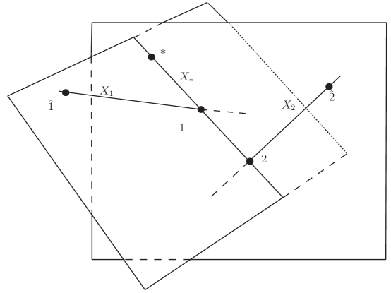
which is supported only on the set , as each form in this wedge product represents a delta-function. The first factor demands that lie in the plane defined by and the line ; call this plane . Identical reasoning tells us that the other factor restricts to lying in the plane . Now, it is obvious that the planes and must intersect in along a line which contains the point . However, given the support of these two factors, this geometric picture is only possible provided and also lie along . In other words, the support of the propagator dictates that , , and all be co-linear in twistor space (see Figure 13).
Hence, modulo some irrelevant numerical factors, our methodology tells us that the twistor space propagator for SYM is:
| (D.23) |
as claimed in the text. Although our derivation here began in Euclidean signature, the result for the full propagator is signature independent and superconformally invariant up to choice of .
References
- [1] E. Witten, Perturbative gauge theory as a string theory in twistor space, Commun.Math.Phys. 252 (2004) 189–258, [hep-th/0312171].
- [2] F. Cachazo, P. Svrcek, and E. Witten, MHV vertices and tree amplitudes in gauge theory, JHEP 0409 (2004) 006, [hep-th/0403047].
- [3] F. Cachazo, P. Svrcek, and E. Witten, Twistor space structure of one-loop amplitudes in gauge theory, JHEP 0410 (2004) 074, [hep-th/0406177].
- [4] F. Cachazo, P. Svrcek, and E. Witten, Gauge theory amplitudes in twistor space and holomorphic anomaly, JHEP 0410 (2004) 077, [hep-th/0409245].
- [5] S. J. Parke and T. R. Taylor, An amplitude for gluon scattering, Physical Review Letters 56 (1986) 2459–2460.
- [6] F. A. Berends and W. T. Giele, Recursive calculations for processes with gluons, Nuclear Physics B 306 (1988) 759.
- [7] K. Risager, A Direct proof of the CSW rules, JHEP 0512 (2005) 003, [hep-th/0508206].
- [8] H. Elvang, D. Z. Freedman, and M. Kiermaier, Recursion Relations, Generating Functions, and Unitarity Sums in N=4 SYM Theory, JHEP 0904 (2009) 009, [arXiv:0808.1720].
- [9] H. Elvang, D. Z. Freedman, and M. Kiermaier, Proof of the MHV vertex expansion for all tree amplitudes in N=4 SYM theory, JHEP 0906 (2009) 068, [arXiv:0811.3624].
- [10] A. Brandhuber, B. J. Spence, and G. Travaglini, One-loop gauge theory amplitudes in N=4 super Yang-Mills from MHV vertices, Nucl.Phys. B706 (2005) 150–180, [hep-th/0407214].
- [11] M. Bullimore, L. Mason, and D. Skinner, MHV Diagrams in Momentum Twistor Space, JHEP 1012 (2010) 032, [arXiv:1009.1854].
- [12] M. Bullimore, MHV Diagrams from an All-Line Recursion Relation, JHEP 1108 (2011) 107, [arXiv:1010.5921].
- [13] A. Hodges, Eliminating spurious poles from gauge-theoretic amplitudes, arXiv:0905.1473.
- [14] L. Mason and D. Skinner, The Complete Planar S-matrix of N=4 SYM as a Wilson Loop in Twistor Space, JHEP 1012 (2010) 018, [arXiv:1009.2225].
- [15] R. Roiban, M. Spradlin, and A. Volovich, On the tree level S matrix of Yang-Mills theory, Phys.Rev. D70 (2004) 026009, [hep-th/0403190].
- [16] D. Skinner, A Direct Proof of BCFW Recursion for Twistor-Strings, JHEP 1101 (2011) 072, [arXiv:1007.0195].
- [17] N. Berkovits and E. Witten, Conformal supergravity in twistor-string theory, JHEP 0408 (2004) 009, [hep-th/0406051].
- [18] S. Gukov, L. Motl, and A. Neitzke, Equivalence of twistor prescriptions for superYang-Mills, Adv.Theor.Math.Phys. 11 (2007) 199–231, [hep-th/0404085].
- [19] L. Mason, Twistor actions for non-self-dual fields: A Derivation of twistor-string theory, JHEP 0510 (2005) 009, [hep-th/0507269].
- [20] R. Boels, L. Mason, and D. Skinner, Supersymmetric Gauge Theories in Twistor Space, JHEP 0702 (2007) 014, [hep-th/0604040].
- [21] L. Mason and D. Skinner, Heterotic twistor-string theory, Nucl.Phys. B795 (2008) 105–137, [arXiv:0708.2276].
- [22] W. Jiang, Aspects of Yang-Mills Theory in Twistor Space. PhD thesis, University of Oxford, 2008. arXiv:0809.0328.
- [23] P. Mansfield, The Lagrangian origin of MHV rules, JHEP 0603 (2006) 037, [hep-th/0511264].
- [24] C. Lovelace, Twistors versus harmonics, arXiv:1006.4289.
- [25] R. Boels, L. Mason, and D. Skinner, From twistor actions to MHV diagrams, Phys.Lett. B648 (2007) 90–96, [hep-th/0702035].
- [26] L. J. Mason and D. Skinner, Scattering Amplitudes and BCFW Recursion in Twistor Space, JHEP 01 (2010) 064, [arXiv:0903.2083].
- [27] N. Arkani-Hamed, F. Cachazo, C. Cheung, and J. Kaplan, The S-Matrix in Twistor Space, JHEP 1003 (2010) 110, [arXiv:0903.2110].
- [28] I. Bena, Z. Bern, D. A. Kosower, and R. Roiban, Loops in twistor space, Phys.Rev. D71 (2005) 106010, [hep-th/0410054].
- [29] R. Britto, F. Cachazo, and B. Feng, New recursion relations for tree amplitudes of gluons, Nucl.Phys. B715 (2005) 499–522, [hep-th/0412308].
- [30] R. Britto, F. Cachazo, B. Feng, and E. Witten, Direct proof of tree-level recursion relation in Yang-Mills theory, Phys.Rev.Lett. 94 (2005) 181602, [hep-th/0501052].
- [31] G. P. Korchemsky and E. Sokatchev, Superconformal invariants for scattering amplitudes in N=4 SYM theory, Nucl. Phys. B839 (2010) 377–419, [arXiv:1002.4625].
- [32] M. Bullimore, L. Mason, and D. Skinner, Twistor-Strings, Grassmannians and Leading Singularities, JHEP 1003 (2010) 070, [arXiv:0912.0539].
- [33] N. Arkani-Hamed, F. Cachazo, C. Cheung, and J. Kaplan, A Duality For The S Matrix, JHEP 1003 (2010) 020, [arXiv:0907.5418].
- [34] L. Mason and D. Skinner, Dual Superconformal Invariance, Momentum Twistors and Grassmannians, JHEP 0911 (2009) 045, [arXiv:0909.0250].
- [35] S. A. Huggett and K. P. Tod, An Introduction to Twistor Theory. Cambridge University Press, 1985.
- [36] R. S. Ward and R. O. Wells, Twistor Geometry and Field Theory. Cambridge University Press, 1990.
- [37] G. Chalmers and W. Siegel, The self-dual sector of QCD amplitudes, Phys. Rev. D. 54 (1996) 7628.
- [38] Y. I. Manin, Gauge Field Theory and Complex Geometry. Springer-Verlag, 2 ed., 1997.
- [39] N. M. J. Woodhouse, Real methods in twistor theory, Classical and Quantum Gravity 2 (1985) 257–291.
- [40] A. Hodges, 1.5.11 Elemental States, in Further Advances in Twistor Theory Vol I: The Penrose Transform and its applications (E. L. J. M. . L. P. Hughston, ed.), vol. 231. Longman Scientific and Technical, 1990.
- [41] J. Drummond, J. Henn, G. Korchemsky, and E. Sokatchev, Dual superconformal symmetry of scattering amplitudes in N=4 super-Yang-Mills theory, Nucl.Phys. B828 (2010) 317–374, [arXiv:0807.1095].
- [42] V. P. Nair, A current algebra for some gauge theory amplitudes, Phys. Lett. B214 (1988) 215.
- [43] E. Witten, Parity invariance for strings in twistor space, Adv.Theor.Math.Phys. 8 (2004) 779–796, [hep-th/0403199].
- [44] M. Atiyah, Green’s functions for self-dual four-manifolds, Advances in Math. Supplementary Studies 7A (1981) 129–158.
- [45] N. Beisert, J. Henn, T. McLoughlin, and J. Plefka, One-Loop Superconformal and Yangian Symmetries of Scattering Amplitudes in N=4 Super Yang-Mills, JHEP 1004 (2010) 085, [arXiv:1002.1733].
- [46] L. F. Alday and J. M. Maldacena, Gluon scattering amplitudes at strong coupling, JHEP 0706 (2007) 064, [arXiv:0705.0303].
- [47] J. Drummond, J. Henn, V. Smirnov, and E. Sokatchev, Magic identities for conformal four-point integrals, JHEP 0701 (2007) 064, [hep-th/0607160].
- [48] J. Drummond, J. Henn, G. Korchemsky, and E. Sokatchev, On planar gluon amplitudes/Wilson loops duality, Nucl.Phys. B795 (2008) 52–68, [arXiv:0709.2368].
- [49] A. Brandhuber, P. Heslop, and G. Travaglini, A Note on dual superconformal symmetry of the N=4 super Yang-Mills S-matrix, Phys.Rev. D78 (2008) 125005, [arXiv:0807.4097].
- [50] A. Brandhuber, P. Heslop, and G. Travaglini, One-Loop Amplitudes in N=4 Super Yang-Mills and Anomalous Dual Conformal Symmetry, JHEP 0908 (2009) 095, [arXiv:0905.4377].
- [51] N. Arkani-Hamed, J. L. Bourjaily, F. Cachazo, S. Caron-Huot, and J. Trnka, The All-Loop Integrand For Scattering Amplitudes in Planar N=4 SYM, JHEP 1101 (2011) 041, [arXiv:1008.2958].
- [52] R. H. Boels, On BCFW shifts of integrands and integrals, JHEP 1011 (2010) 113, [arXiv:1008.3101].
- [53] M. Bullimore and D. Skinner, Holomorphic Linking, Loop Equations and Scattering Amplitudes in Twistor Space, arXiv:1101.1329.
- [54] L. F. Alday, J. M. Henn, J. Plefka, and T. Schuster, Scattering into the fifth dimension of N=4 super Yang-Mills, JHEP 1001 (2010) 077, [arXiv:0908.0684].
- [55] L. F. Alday, D. Gaiotto, J. Maldacena, A. Sever, and P. Vieira, An Operator Product Expansion for Polygonal null Wilson Loops, JHEP 1104 (2011) 088, [arXiv:1006.2788].
- [56] A. B. Goncharov, M. Spradlin, C. Vergu, and A. Volovich, Classical Polylogarithms for Amplitudes and Wilson Loops, Phys.Rev.Lett. 105 (2010) 151605, [arXiv:1006.5703].
- [57] D. Gaiotto, J. Maldacena, A. Sever, and P. Vieira, Pulling the straps of polygons, JHEP 1112 (2011) 011, [arXiv:1102.0062].
- [58] N. Arkani-Hamed, J. Bourjaily, F. Cachazo, and J. Trnka, Unification of Residues and Grassmannian Dualities, JHEP 1101 (2011) 049, [arXiv:0912.4912].
- [59] N. Arkani-Hamed, J. Bourjaily, F. Cachazo, and J. Trnka, Local Spacetime Physics from the Grassmannian, JHEP 1101 (2011) 108, [arXiv:0912.3249].
- [60] N. Arkani-Hamed, J. L. Bourjaily, F. Cachazo, and J. Trnka, Local Integrals for Planar Scattering Amplitudes, arXiv:1012.6032.