Abstract

We discuss Higgs boson decays in the CP-violating MSSM, and examine their phenomenological impact using cross section limits from the LEP Higgs searches. This includes a discussion of the full 1-loop results for the partial decay widths of neutral Higgs bosons into lighter neutral Higgs bosons ($h_{a}\to h_{b}h_{c}$) and of neutral Higgs bosons into fermions ($h_{a}\to f\bar{f}$). In calculating the genuine vertex corrections, we take into account the full spectrum of supersymmetric particles and all complex phases of the supersymmetric parameters. These genuine vertex corrections are supplemented with Higgs propagator corrections incorporating the full one-loop and the dominant two-loop contributions, and we illustrate a method of consistently treating diagrams involving mixing with Goldstone and Z bosons. In particular, the genuine vertex corrections to the process $h_{a}\to h_{b}h_{c}$ are found to be very large and, where this process is kinematically allowed, can have a significant effect on the regions of the CPX benchmark scenario which can be excluded by the results of the Higgs searches at LEP. However, there remains an unexcluded region of CPX parameter space at a lightest neutral Higgs boson mass of $\sim 45\,\,\mathrm{GeV}$. In the analysis, we pay particular attention to the conversion between parameters defined in different renormalisation schemes and are therefore able to make a comparison to the results found using renormalisation group improved/effective potential calculations.

1 Introduction

High energy colliders, at present and in the past, have given the search for Higgs bosons a high priority. The LEP and Tevatron experiments, in particular, have been able to turn the non-observation of Higgs bosons into constraints on the Higgs sector, which have been very useful in reducing the available parameter space of some of the most popular particle physics models, such as the Standard Model (SM) [1] and the Minimal Supersymmetric Standard Model (MSSM) [2]. For first results on the Higgs searches at the LHC, see Refs. [3, 4].

However, MSSM scenarios involving CP violation in the Higgs sector, which induces a mixing of all three neutral Higgs bosons, can prove particularly difficult to restrict using the Higgs search data. This is due to the fact that the CP violation can result in suppressed couplings of the lightest Higgs boson to two gauge bosons and to the non-standard decay mode of a heavier SM-like Higgs boson into a pair of light Higgs bosons, resulting in an experimentally rather challenging final state. The $\rm{CPX}$ benchmark scenario [5] is an example of such a situation in the MSSM. In the original combined LEP analysis by the LEP Higgs Working group and the LEP collaborations (LHWG), it was found that substantial regions of the $\rm{CPX}$ parameter space could not be excluded [2] where the lightest Higgs mass is substantially below the limit on the Standard Model Higgs mass [1] of $M_{H}=114.4\,\,\mathrm{GeV}$.

In this paper, we will present complete one-loop results for the decay widths of neutral Higgs bosons into lighter neutral Higgs bosons (Higgs cascade decays) and the decay widths of neutral Higgs bosons into fermions in the CP-violating MSSM. The results are obtained in the Feynman-diagrammatic approach, taking into account the full dependence on the spectrum of supersymmetric particles and all complex phases of the supersymmetric parameters. The genuine vertex contributions are supplemented with two-loop propagator-type corrections, yielding the currently most precise prediction for this class of processes. One-loop propagator-type mixing between neutral Higgs bosons and Goldstone and Z bosons is also consistently taken into account.

Both of these calculations require loop corrections to the neutral Higgs mass matrix ${\mathbf{M}}$, which are well known for the real and complex MSSM and are frequently used to add propagator corrections to processes involving external neutral Higgs particles. These corrections are incorporated in the two main public codes for calculating the complex MSSM Higgs sector, FeynHiggs [6, 7, 8, 9, 10] and CPsuperH [11, 12]. FeynHiggs is based on the Feynman-diagrammatic approach and on-shell mass renormalisation while CPsuperH is based on a renormalisation group improved effective potential calculation and $\overline{\rm{DR}}$ renormalisation. Therefore, to compare between these results it is necessary to perform a parameter conversion. We shall discuss this issue in Sect. 5. We also investigate the numerical impact of parametrising the neutral Higgs self-energies (in the Feynman-diagrammatic approach) in terms of the $\overline{\rm{MS}}$ top mass, rather than the on-shell top mass, which is formally a 3-loop effect.

The Higgs cascade decays often dominate the Higgs decay width where they are kinematically allowed. They directly involve the Higgs self-couplings, the observation and measurement of which is a crucial goal for the experimental confirmation of the Higgs mechanism. We will present two momentum-dependent approximations for the loop-corrected triple Higgs couplings, which can be used, for instance, for predictions of the Higgs production process $e^{+}e^{-}\to Zh_{a}h_{a}$ at the ILC [13] or CLIC [14].

The genuine vertex corrections to the triple Higgs decay can be very large. In the MSSM with real parameters, the leading Yukawa vertex corrections and the complete 1-loop vertex corrections have been calculated [15, 16, 17, 18, 19, 20, 21]. However, for the complex MSSM, previous to our result, first described in Ref. [22], only effective coupling approximations were available [23, 24], as provided by the program CPsuperH [11, 12]. The genuine vertex corrections we present will be incorporated into the code FeynHiggs. As we will demonstrate, the $h_{2}\to h_{1}h_{1}$ decay width has a critical influence on the size and shape of one of the regions of $\rm{CPX}$ parameter space which the LEP Higgs search results are unable to exclude.

The fermionic decay modes of the neutral Higgs bosons are crucially important to collider phenomenology. These modes have been used when obtaining a lower bound on the Standard Model Higgs mass [1] and to exclude significant regions of the MSSM parameter space [2, 25, 26]. In particular, an accurate prediction for the Higgs decay to b-quarks has been vital for these analyses, since, for Standard Model Higgs bosons with mass less than about $130\,\,\mathrm{GeV}$ and for most SUSY scenarios, $h_{a}\to b\bar{b}$ is the dominant decay mode. The decay to $\tau$-leptons can also be very important for Higgs searches, as demonstrated for instance for various benchmark MSSM scenarios in the high $\tan\beta$ region at the Tevatron [27].

In the Standard Model, the fermionic decay width is extremely well known (for a review, see e.g. Ref. [28] and references therein), and the treatment of higher-order QCD (gluon-exchange) and QED corrections can be taken over to the MSSM case. The SUSY QCD corrections can be sizable for the $h_{a}\to b\bar{b}$ decay and should be resummed (see, for example, Ref. [29], for an investigation into these effects). Results supplemented with leading 2-loop propagator corrections [30] and full electroweak contributions [31] are also available in the MSSM with real parameters.

Predictions for the $h_{a}\to f\bar{f}$ decay widths for the Standard Model and the MSSM with real parameters can be obtained from the programs HDECAY [32] and HFOLD [33]. For the complex MSSM, the program CPsuperH [11, 12] is available. It is based on calculations involving effective $h_{a}f\bar{f}$ couplings, as described in Ref. [24].

The program FeynHiggs [6, 7, 8, 9, 10] calculates the $h_{a}\to f\bar{f}$ decay width using the Feynman-diagrammatic approach, including the most significant QCD corrections, resummed SUSY QCD corrections and propagator corrections incorporating the full neutral Higgs self-energies. This calculation is valid in the real and complex MSSM. The full 1-loop electroweak vertex corrections presented here have recently been incorporated into FeynHiggs.

The corrections to the Higgsstrahlung and Higgs pair production processes at LEP in the MSSM with real parameters have been studied in Refs. [34, 35, 36, 37, 38, 39] and the CP-violating MSSM in Refs. [40, 41, 42, 43, 44]. In the present paper, we will investigate the $t,\tilde{t},b,\tilde{b}$ corrections to these production processes in the Feynman-diagrammatic approach in the CP-violating MSSM, and supplement these with full propagator-type corrections. This type of corrections were not included in the Feynman-diagrammatic analysis of the $\rm{CPX}$ scenario in Ref. [2].

The parameter region in the MSSM with complex parameters that could not be excluded with the Higgs searches at LEP, characterised by a rather light Higgs boson with a mass of about $45\,\,\mathrm{GeV}$ and moderate values of $\tan\beta$, persists also in view of the present search limits from the Tevatron [27]. This parameter region will be difficult to cover also with the standard Higgs search channels at the LHC [45, 46, 47], while it can be thoroughly investigated at the ILC [13]. The phenomenology of scenarios with such a light Higgs boson has recently found considerable interest in the literature, see Refs. [48, 49, 50, 51, 52, 53, 54, 55, 56] for discussions of other (non-standard) possible LHC search channels to access this parameter region.

In the present paper we make use of our improved theoretical predictions for the Higgs branching ratios into a pair of lighter Higgs bosons and into a fermion pair to examine their impact on the parameter region with a light Higgs boson left unexcluded by the LEP Higgs searches. For this purpose we employ the topological cross section limits obtained at LEP, as implemented in the program HiggsBounds [57, 58]. We investigate the sensitivity of the excluded parameter region with respect to variations in the parameters of the $\rm{CPX}$ scenario. This analysis updates and considerably extends our previous results reported in Ref. [22]. We then compare our results to the results obtained with the code CPsuperH, using various ways of performing the parameter conversion.

The paper is organized as follows: After introducing complex parameters in Sect. 2 and the CPX scenario in Sect. 3 we discuss contributions to the Higgs masses and mixings including also resummed SUSY QCD corrections in Sect. 4. In Sect. 5 we focus on the conversion between different renormalization schemes as well as on the effect of a different parameterization of the top quark mass. In Sect. 6 and in Sect. 7 we discuss the Higgs cascade decay and the Higgs decay into SM fermions, respectively, and the different contributions to their partial decay widths and possible approximations. After the investigation of the partial decay widths we turn our focus particularly on the branching ratios of the Higgs cascade decay processes in Sect. 8. In Sect. 9 Higgs production channels which were relevant at LEP are investigated. Finally, in Sect. 10 we discuss the phenomenological impact of the improved predictions obtained in this paper. We investigate in particular the parameter dependence of the CPX scenario and we perform a thorough comparison with the results obtained with the program CPsuperH. Sect. 11 contains our conclusions.

2 The MSSM with complex parameters at tree level

In its general form, the MSSM allows various parameters to be complex. This includes the trilinear couplings $A_{f}$, the Higgsino mass parameter $\mu$, the gluino mass parameter $M_{3}$ and the soft SUSY breaking parameters $M_{1}$ and $M_{2}$ from the neutralino/chargino sector. These complex parameters can induce CP violation. Below we list the relevant quantities to fix our notation, which closely follows that in Ref. [7].

We write the two MSSM Higgs doublets as

$${\cal H}_{1}=\begin{pmatrix}H_{11}\\ H_{12}\end{pmatrix} =\begin{pmatrix}v_{1}+\tfrac{1}{\sqrt{2}}(\phi_{1}-i\chi_{1})\\ -\phi^{-}_{1}\end{pmatrix},$$

$${\cal H}_{2}=\begin{pmatrix}H_{21}\\ H_{22}\end{pmatrix} =\begin{pmatrix}\phi^{+}_{2}\\ v_{2}+\tfrac{1}{\sqrt{2}}(\phi_{2}+i\chi_{2})\end{pmatrix},$$ (1)

where $v_{1}$ and $v_{2}$ are the vacuum expectation values, and $\tan\beta\equiv v_{2}/v_{1}$. Here we have made use of the fact that the MSSM Higgs sector is CP-conserving at lowest order, i.e. complex phases occurring in the Higgs potential can be rotated away (or vanish via the minimisation of the Higgs potential).

The tree level neutral mass eigenstates $h,H,A,G$ are related to the tree level neutral fields $\phi_{1},\phi_{2},\chi_{1},\chi_{2}$ through a unitary matrix,

$$\begin{pmatrix}h\\ H\\ A\\ G\end{pmatrix}=\begin{pmatrix}-\sin\alpha\,&\cos\alpha\,&0&0\\ \quad\cos\alpha\,&\sin\alpha\,&0&0\\ 0&0&-\sin\beta_{\mathrm{n}}&\cos\beta_{\mathrm{n}}\\ 0&0&\quad\cos\beta_{\mathrm{n}}&\sin\beta_{\mathrm{n}}\end{pmatrix}\cdot\begin{pmatrix}\phi_{1}\\ \phi_{2}\\ \chi_{1}\\ \chi_{2}\end{pmatrix},$$ (2)

in which the CP-even eigenstates $\phi_{1},\phi_{2}$ do not mix with the CP-odd eigenstates $\chi_{1},\chi_{2}$. Unless otherwise stated, $h,H,A,G$ will always represent tree level neutral (mass eigenstate) fields throughout this paper. At tree level, the off-diagonal mass terms must vanish, leading to the condition $\beta_{\mathrm{n}}=\beta$.

The Higgs sector at lowest order is given in terms of two independent parameters (besides the gauge couplings), conventionally chosen as $\tan\beta$ and either $m_{A}$ or $m_{H^{\pm}}$. Since CP violation can be induced via potentially large higher-order corrections, in general all three neutral Higgs bosons will mix once higher-order corrections are included, so that the CP-odd $A$ boson is no longer a mass eigenstate. For the general case of the MSSM with complex parameters it is therefore convenient to use $m_{H^{\pm}}$ as input parameter. In our notation lower-case Higgs masses indicate tree-level masses, while upper case masses refer to loop-corrected masses.

We write the squark mass matrices as

$$M_{\tilde{q}}=\begin{pmatrix}M_{L}^{2}+m_{q}^{2}+M_{Z}^{2}\cos 2\beta(I_{3}^{q}-Q_{q}s_{\mathrm{w}}^{2})&m_{q}\;X_{q}^{*}\\ m_{q}\;X_{q}&M_{\tilde{q}_{R}}^{2}+m_{q}^{2}+M_{Z}^{2}\cos 2\beta Q_{q}s_{\mathrm{w}}^{2}\end{pmatrix},$$ (3)

where

$$X_{q} = A_{q}-\mu^{*}\{\cot\beta,\tan\beta\},$$ (4)

and $\cot\beta$ or $\tan\beta$ applies to u-type or d-type quarks, respectively. The eigenvalues of eq. (3) are

$$m_{\tilde{q}_{1,2}}^{2}=m_{q}^{2}+\frac{1}{2} \Bigl{[}M_{L}^{2}+M_{\tilde{q}_{R}}^{2}+I_{3}^{q}M_{Z}^{2}\cos 2\beta$$

$$\mp\sqrt{[M_{L}^{2}-M_{\tilde{q}_{R}}^{2}+M_{Z}^{2}\cos 2\beta(I_{3}^{q}-2Q_{q}s_{\mathrm{w}}^{2})]^{2}+4m_{q}^{2}|X_{q}|^{2}}~{}\Bigr{]}.$$ (5)

In the complex MSSM, the trilinear coupling $A_{q}$ and the higgsino mass parameter $\mu$ can have non-zero complex phases. The mass matrix $M_{\tilde{q}}$ can be diagonalised by the matrix ${\mathbf{U}}_{\tilde{q}}$. Here

$$\left(\begin{array}[]{c}\tilde{q}_{1}\\ \tilde{q}_{2}\end{array}\right)={\mathbf{U}}_{\tilde{q}}\left(\begin{array}[]{c}\tilde{q}_{L}\\ \tilde{q}_{R}\end{array}\right), {\rm where} {\mathbf{U}}_{\tilde{q}}=\left(\begin{array}[]{cc}c_{\tilde{q}}&s_{\tilde{q}}\\ -s_{\tilde{q}}^{*}&c_{\tilde{q}}\end{array}\right),$$ (12)

and $c_{\tilde{q}}$ is real, $s_{\tilde{q}}$ is complex, and $c_{\tilde{q}}^{2}+|s_{\tilde{q}}|^{2}=1$.

The coefficient of the gluino mass term in the Lagrangian, $M_{3}$, is in general complex. The gluino mass is given by $m_{\tilde{g}}=|M_{3}|$, while the phase $\phi_{M_{3}}$ can be absorbed into the gluino fields [59]. The phase of $M_{3}$ thus appears in the quark–squark–gluino couplings.

For the chargino mass matrix we use

$${\mathbf{M_{\rm chargino}}}=\begin{pmatrix}M_{2}&\sqrt{2}\sin\beta\,M_{W}\\ \sqrt{2}\cos\beta\,M_{W}&\mu\end{pmatrix},$$ (13)

which includes the soft SUSY-breaking term $M_{2}$, which can be complex. For the neutralino mass matrix we use

$${\mathbf{M_{\rm neutralino}}}=\begin{pmatrix}M_{1}&0&-M_{Z}\,s_{\mathrm{w}}\cos\beta\,&M_{Z}\,s_{\mathrm{w}}\sin\beta\,\\ 0&M_{2}&\quad M_{Z}\,c_{\mathrm{w}}\cos\beta\,&M_{Z}\,c_{\mathrm{w}}\sin\beta\,\\ -M_{Z}\,s_{\mathrm{w}}\cos\beta\,&M_{Z}\,c_{\mathrm{w}}\cos\beta\,&0&-\mu\\ \quad M_{Z}\,s_{\mathrm{w}}\sin\beta\,&M_{Z}\,c_{\mathrm{w}}\sin\beta\,&-\mu&0\end{pmatrix},$$ (14)

which includes furthermore the soft SUSY-breaking term $M_{1}$, which can also be complex.

It should be noted that not all phases mentioned above are physical, but only certain combinations. In particular, the phase of the parameter $M_{2}$ (chosen by convention) and, as mentioned above, the phase appearing in the Higgs sector at lowest order can be rotated away.

3 Phenomenology and the $\rm{CPX}$ scenario

CP-violating effects, which can enter the Higgs sector via potentially large higher-order corrections, can give rise to important phenomenological consequences. CP phases in the loop corrections to the Higgs particles can have a large impact on the predictions for the masses (all three neutral Higgs bosons mix in the CP-violating case) and the Higgs couplings [60, 61, 62, 41, 7].

Studies of the possible impact of CP-violating effects on the MSSM Higgs sector have often been carried out in the CPX benchmark scenario [5]. As input values for the CPX scenario we use in this paper

• $m_{t}=173.1\,\,\mathrm{GeV}$

• $M_{\rm SUSY}=500\,\,\mathrm{GeV}(=M_{L}^{\rm on-shell}=M_{\tilde{q}_{R}}^{\rm on-shell})$

• $\mu=2000\,\,\mathrm{GeV}$

• $|M_{3}|=1000\,\,\mathrm{GeV}$

• $M_{2}=200\,\,\mathrm{GeV}$, $M_{1}=\frac{5}{3}\frac{s_{W}^{2}}{c_{W}^{2}}M_{2}$ (see e.g. Ref. [63]).

• $|A_{t}^{\rm on-shell}|=|A_{b}|=900\,\,\mathrm{GeV}$

• $\phi_{A_{t}^{\rm on-shell}}=\phi_{A_{b}}=\phi_{M_{3}}=\frac{\pi}{2}$

• $M_{H^{\pm}}\leq 1000\,\,\mathrm{GeV}$

With the phases of the parameters $A_{t,b}$ and $M_{3}$ set to the maximal value of $\pi/2$ and the relatively large value of $\mu$, this scenario has been devised to illustrate the possible importance of CP-violating effects.

The above values differ from the ones defined in Ref. [5] in the following ways: Firstly, we use an on-shell value for the absolute value of the trilinear coupling $A_{t}$ and the soft SUSY breaking mass parameters $M_{L}$ and $M_{\tilde{q}_{R}}$, rather than $\overline{\rm{DR}}$ values, and we therefore use a numerical value of $|A_{t}|$ that is somewhat shifted compared to that specified in Ref. [5] in order to remain in an area of parameter space with similar phenomenology (the value specified in Ref. [5] is $|A_{t}^{\overline{\rm{DR}}}|=1000\,\,\mathrm{GeV}$). Secondly, we use $m_{t}=173.1\,\,\mathrm{GeV}$, which was the world average top-quark mass in March 2009 [64].

We use an on-shell definition of $A_{t}$, $M_{L}$ and $M_{\tilde{q}_{R}}$ since this is the natural choice for a Feynman-diagrammatic calculation. We will discuss how to convert between the different parameter definitions in Sect. 5. For the purposes of this discussion, we use a second scenario using the parameter values given above, except with $A_{t}$, $M_{L}$, $M_{\tilde{q}_{R}}$ defined according to the $\overline{\rm{DR}}$ scheme at the scale $M_{S}:=\sqrt{M_{\rm SUSY}^{2}+m_{t}^{2}}$ and with $|A_{t}^{\overline{\rm{DR}}}(M_{S})|=1000\,\,\mathrm{GeV}(=|A_{b}|)$, $\phi_{A_{t}^{\overline{\rm{DR}}}}(M_{S})=\frac{\pi}{2}$, $M_{L}^{\overline{\rm{DR}}}(M_{S})=500\,\,\mathrm{GeV}$ and $M_{\tilde{q}_{R}}^{\overline{\rm{DR}}}(M_{S})=500\,\,\mathrm{GeV}$, which we will call the $\overline{\rm{CPX}}$ scenario (i.e. this scenario is more similar to that in Ref. [5]).

The LEP Higgs Working Group study[2] of the CPX scenario also used $|A_{t}^{\overline{\rm{DR}}}|=1000\,\,\mathrm{GeV}$. The majority of its analyses were performed using $m_{t}=174.3\,\,\mathrm{GeV}$. We will investigate the dependence of our results on $m_{t}$ in Sect. 10.2.

It should be noted that there are constraints on the CP phases in the complex MSSM from experimentally measured upper limits on electric dipole moments, such as those of the electron and neutron (for a recent discussion, see e.g. Ref. [65]). These provide particularly significant constraints on the CP phases in the first two generations. The constraints on the phases of the third generation are less restrictive. In the definition of the CPX benchmark scenario, existing bounds on CP phases were taken into account, see Ref. [41] for more details.

4 Loop corrections to the Higgs masses and Higgs mixing matrices

Higher-order corrections to Higgs masses and mixing properties are known to be very important for the phenomenology of the MSSM Higgs sector, see Refs. [66, 67, 68] for reviews.

In the MSSM with real parameters, the full 1-loop result [69, 70, 71, 72, 73, 34, 31, 74] and the dominant 2-loop corrections [9, 75, 76, 77, 78, 79, 80, 81, 82, 83, 84, 85, 86, 87, 88, 89] have been calculated, and the $\tan\beta$-enhanced terms ${\cal O}(\alpha_{b}(\alpha_{s}\tan\beta)^{n})$ have been resummed [90, 91, 92, 29, 93, 94]. A full 2-loop effective potential calculation is known [95, 96, 97, 98, 99, 100, 101, 102]. In addition, some dominant 3-loop contributions have been calculated [103, 104, 105].

In the complex MSSM, 1-loop corrections from the fermion/sfermion sector and some leading logarithmic corrections from the gaugino sector and the dominant 2-loop results have been calculated in the renormalisation group improved effective potential approach [106, 62, 60, 41, 107, 108, 97, 100, 104]. In the Feynman-diagrammatic approach, leading 1-loop contributions have been obtained in Ref. [61, 109], and the full 1-loop result has been calculated in Ref. [7]. At 2-loop order, the $\mathcal{O}(\alpha_{t}\alpha_{s})$ corrections are available [110].

Most of these results for the complex MSSM have been incorporated either into the public code FeynHiggs [7, 8, 9, 10, 111, 112, 113], which uses the Feynman-diagrammatic approach, or the public code CPsuperH [11, 12], which uses the renormalisation group improved effective potential approach.

In this paper, when calculating the Higgs masses and mixings, we will use renormalised neutral Higgs self-energies calculated by FeynHiggs, to take advantage of the fact that it includes the complete 1-loop result and ${\cal O}(\alpha_{t}\alpha_{s})$ corrections of Ref. [110] with full phase dependence. FeynHiggs additionally allows the option of including sub-leading 2-loop corrections which are known so far only for the MSSM with real parameters [82, 85, 83, 86, 76]. If the user wishes to apply these corrections in an MSSM calculation with complex phases, FeynHiggs evaluates these corrections at a phase of $0$ and $\pi$ for each complex parameter, then an interpolation is performed to arrive at an approximation to these corrections for arbitrary complex phases. However, this prescription can be problematic in a rather ‘extreme’ scenario like the CPX scenario. In fact, it can happen in this case that one of the combinations of real parameters needed as input for the interpolation turns out to be in an unstable region of the parameter space where the reliability of the perturbative predictions is questionable. This would skew the interpolation towards the unstable values. Therefore, unless otherwise stated, we will use in the present paper the leading ${\cal O}(\alpha_{t}\alpha_{s})$ corrections to the Higgs self-energies from FeynHiggs, but not the sub-leading 2-loop corrections. A discussion of the incorporation of the subleading 2-loop contributions via the interpolation from the results for real parameters is given in Sect. 10.3. As discussed in more detail below, besides the irreducible 2-loop contributions of ${\cal O}(\alpha_{t}\alpha_{s})$ we do incorporate into our results higher order $\tan\beta$–enhanced terms (for arbitrary complex parameters), which we take into account by introducing an effective b-quark mass.

4.1 Determination of neutral Higgs masses

In general, the neutral Higgs masses are obtained from the real parts of the complex poles of the propagator matrix. In the determination of the Higgs masses, we neglect mixing with the Goldstone and Z bosons as these are sub-leading 2-loop contributions to the Higgs masses. We therefore use a $3\times 3$ propagator matrix ${\mathbf{\Delta}}(p^{2})$ in the $(h,H,A)$ basis.

In order to determine the neutral Higgs masses we must first find the three solutions to

$$\left|{\mathbf{\Delta}}^{-1}(p^{2})\right|=0,$$ (15)

which, in the case with non-zero mixing between all three neutral Higgs bosons, is equivalent to solving

$$\frac{1}{\Delta_{ii}(p^{2})}=0,$$ (16)

where $i=h,H$ or $A$. The propagator matrix is related to the $3\times 3$ matrix of the irreducible 2-point vertex-functions ${\mathbf{\hat{\Gamma}}}_{2}(p^{2})$ through the equation

$$\left[-{\mathbf{\Delta}}(p^{2})\right]^{-1}={\mathbf{\hat{\Gamma}}}_{2}(p^{2})=i\left[p^{2}{\rm 1\kern-1.19995pt\rule{0.3pt}{6.45831pt}\raisebox{0.0pt}{\rule{1.00006pt}{0.3pt}}}-{\mathbf{M}}(p^{2})\right],$$ (17)

where

$${\mathbf{M}}(p^{2}) =\begin{pmatrix}m_{h}^{2}-\hat{\Sigma}_{hh}(p^{2})&-\hat{\Sigma}_{hH}(p^{2})&-\hat{\Sigma}_{hA}(p^{2})\\ -\hat{\Sigma}_{hH}(p^{2})&m_{H}^{2}-\hat{\Sigma}_{HH}(p^{2})&-\hat{\Sigma}_{HA}(p^{2})\\ -\hat{\Sigma}_{hA}(p^{2})&-\hat{\Sigma}_{HA}(p^{2})&m_{A}^{2}-\hat{\Sigma}_{AA}(p^{2})\end{pmatrix}.$$ (18)

As before, $m_{h}$,$m_{H}$,$m_{A}$ refer to the tree level masses. $\hat{\Sigma}_{ij}(p^{2})$ are renormalised Higgs self-energies. The explicit form of the counterterms used in this paper is given in App. B. For the majority of these renormalisation conditions, we use the on-shell scheme. However, we shall use $\overline{\rm{DR}}$ renormalisation for the Higgs fields (see Ref. [7]). If there is CP conservation, $\hat{\Sigma}_{hA}(p^{2})=\hat{\Sigma}_{HA}(p^{2})=0$, and the CP-even Higgs bosons $h,H$ do not mix with the CP-odd Higgs boson $A$.

In general, the renormalised Higgs self-energies can be complex, due to absorptive parts. Therefore, the three poles of the propagator matrix ${\cal M}_{a}^{2}$ can be written as

$${\cal M}_{h_{a}}^{2}=M_{h_{a}}^{2}-iM_{h_{a}}W_{h_{a}},$$ (19)

where $M_{h_{a}}$ is real and is interpreted as the loop-corrected (i.e. physical) mass, $W_{h_{a}}$ is the Higgs width, and $a=1,2,3$.

In the MSSM with complex parameters, the loop-corrected masses are labelled in size order such that

$$M_{h_{1}}\leq M_{h_{2}}\leq M_{h_{3}}.$$ (20)

In the CP-conserving case, the masses are labelled such that the CP-even loop-corrected Higgs bosons have masses $M_{h}$ and $M_{H}$ with $M_{h}\leq M_{H}$ and the CP-odd loop-corrected Higgs boson has mass $M_{A}$ (the numerical value of $M_{A}$ is affected by loop corrections only if $M_{H^{\pm}}$ is chosen as an independent input parameter).

Solving eq. (15) with full momentum dependence involves an iterative procedure, since the self-energies also depend on the momentum. In order to deal with the complex momentum argument it is convenient to use an expansion about the real part of the pole, $M^{2}_{h_{a}}$, such that

$$\hat{\Sigma}_{jk}({\cal M}_{h_{a}}^{2}) \simeq \hat{\Sigma}_{jk}(M_{h_{a}}^{2})+i\mbox{Im}\,\left[{\cal M}_{h_{a}}^{2}\right]\hat{\Sigma}_{jk}^{\prime}(M_{h_{a}}^{2}),$$ (21)

with $j=h,H,A$ and $k=h,H,A$. We obtain $\hat{\Sigma}_{jk}(M_{h_{a}}^{2})$ and $\hat{\Sigma}_{jk}^{\prime}(M_{h_{a}}^{2})$ (where the prime indicates the derivative w.r.t. the external momentum squared) from FeynHiggs [6, 7, 8, 9, 10]. For each $h_{a}$, we use a momentum-independent approximation to obtain an initial value for the iteration. This solution is then refined using

$${\cal M}_{h_{a}}^{2,\left[n+1\right]} = \mbox{ $a$th eigenvalue of }{\mathbf{M}}({\cal M}_{h_{a}}^{2,\left[n\right]}),$$ (22)

where the eigenvalues have been sorted into ascending value, according to their real parts. We check the validity of the truncation of the expansion in eq. (21) by performing an iteration using an expansion up to second order:

$$\hat{\Sigma}_{jk}({\cal M}_{h_{a}}^{2}) \simeq \hat{\Sigma}_{jk}(M_{h_{a}}^{2})+i\mbox{Im}\,\left[{\cal M}_{h_{a}}^{2}\right]\hat{\Sigma}_{jk}^{\prime}(M_{h_{a}}^{2})$$ (23)

$$+ \frac{1}{2}\left(i\mbox{Im}\,\left[{\cal M}_{h_{a}}^{2}\right]\hat{\Sigma}_{jk}^{\prime\prime}(M_{h_{a}}^{2})\right)^{2},$$

and confirming that the resultant Higgs masses show no significant changes.

4.2 Wave function normalisation factors

In order to ensure that the S-matrix is correctly normalised, the residues of the propagators have to be set to one. We achieve this by including finite wave function normalisation factors which are composed of the renormalised self-energies. These ‘Z-factors’ can be collected in to a matrix ${\mathbf{\hat{Z}}}$ where

$$\lim_{p^{2}\to{\cal M}_{h_{a}}^{2}}-\frac{i}{p^{2}-{\cal M}_{h_{a}}^{2}}\left({\mathbf{\hat{Z}}}\cdot{\mathbf{\hat{\Gamma}}}_{2}\cdot{\mathbf{\hat{Z}}}^{T}\right)_{hh} = 1,$$ (24)

$$\lim_{p^{2}\to{\cal M}_{h_{b}}^{2}}-\frac{i}{p^{2}-{\cal M}_{h_{b}}^{2}}\left({\mathbf{\hat{Z}}}\cdot{\mathbf{\hat{\Gamma}}}_{2}\cdot{\mathbf{\hat{Z}}}^{T}\right)_{HH} = 1,$$ (25)

$$\lim_{p^{2}\to{\cal M}_{h_{c}}^{2}}-\frac{i}{p^{2}-{\cal M}_{h_{c}}^{2}}\left({\mathbf{\hat{Z}}}\cdot{\mathbf{\hat{\Gamma}}}_{2}\cdot{\mathbf{\hat{Z}}}^{T}\right)_{AA} = 1,$$ (26)

such that

$$\begin{pmatrix}\hat{\Gamma}_{h_{a}}\\ \hat{\Gamma}_{h_{b}}\\ \hat{\Gamma}_{h_{c}}\end{pmatrix}={\mathbf{\hat{Z}}}\cdot\begin{pmatrix}\hat{\Gamma}_{h}\\ \hat{\Gamma}_{H}\\ \hat{\Gamma}_{A}\end{pmatrix},$$ (27)

where $\hat{\Gamma}_{h_{a}}$ is a one-particle irreducible n-point vertex-function which involves a single external Higgs $h_{a}$, and $h_{a},h_{b},h_{c}=$ some combination of $h_{1},h_{2},h_{3}$.

The matrix ${\mathbf{\hat{Z}}}$ is non-unitary. We write it as

$${\mathbf{\hat{Z}}} =\begin{pmatrix}\sqrt{Z_{h}}&\sqrt{Z_{h}}Z_{hH}&\sqrt{Z_{h}}Z_{hA}\\ \sqrt{Z_{H}}Z_{Hh}&\sqrt{Z_{H}}&\sqrt{Z_{H}}Z_{HA}\\ \sqrt{Z_{A}}Z_{Ah}&\sqrt{Z_{A}}Z_{AH}&\sqrt{Z_{A}}\end{pmatrix}.$$ (28)

We find the elements of ${\mathbf{\hat{Z}}}$ by solving eq. (24), which gives

$$Z_{h}=\frac{1}{\left.\frac{\partial}{\partial p^{2}}\left(\frac{i}{\Delta_{hh}(p^{2})}\right)\right|}_{p^{2}={\cal M}_{h_{a}}^{2}}, Z_{H}=\frac{1}{\left.\frac{\partial}{\partial p^{2}}\left(\frac{i}{\Delta_{HH}(p^{2})}\right)\right|}_{p^{2}={\cal M}_{h_{b}}^{2}}, Z_{A}=\frac{1}{\left.\frac{\partial}{\partial p^{2}}\left(\frac{i}{\Delta_{AA}(p^{2})}\right)\right|}_{p^{2}={\cal M}_{h_{c}}^{2}},$$ (29)

$$Z_{hH}=\left.\frac{\Delta_{hH}}{\Delta_{hh}}\right|_{p^{2}={\cal M}_{h_{a}}^{2}}, Z_{Hh}=\left.\frac{\Delta_{hH}}{\Delta_{HH}}\right|_{p^{2}={\cal M}_{h_{b}}^{2}}, Z_{Ah}=\left.\frac{\Delta_{hA}}{\Delta_{AA}}\right|_{p^{2}={\cal M}_{h_{c}}^{2}},$$ (30)

$$Z_{hA}=\left.\frac{\Delta_{hA}}{\Delta_{hh}}\right|_{p^{2}={\cal M}_{h_{a}}^{2}}, Z_{HA}=\left.\frac{\Delta_{HA}}{\Delta_{HH}}\right|_{p^{2}={\cal M}_{h_{b}}^{2}}, Z_{AH}=\left.\frac{\Delta_{HA}}{\Delta_{AA}}\right|_{p^{2}={\cal M}_{h_{c}}^{2}}.$$ (31)

We choose $h_{a}=h_{1}$, $h_{b}=h_{2}$ and $h_{c}=h_{3}$. $Z_{i}$ is, in general, complex. Other choices for the Z-factors are possible, such as that in Ref. [114], where we use the limit $p^{2}=M_{h_{1,2,3}}^{2}$. However, this does not allow the same freedom for choosing $a,b,c$.

Since the elements of ${\mathbf{\hat{Z}}}$ involve evaluating self-energies at complex momenta, we use again the expansion given in eq. (21). In order to make sure that the neglected higher order terms in eq. (21) are small, we also calculate ${\mathbf{\hat{Z}}}$ using eq. (23), and check that this does not significantly change the result.

The wave function normalisation factors are included in the calculation by multiplying the irreducible vertex factor $\hat{\Gamma}$ by ${\mathbf{\hat{Z}}}$ once for each external Higgs boson involved in the process.

4.3 Goldstone or gauge bosons mixing contributions to the Higgs propagators

A complete 1-loop prediction for a process involving a neutral Higgs propagator in the MSSM with complex parameters will, in general, contain terms involving the self-energies $\hat{\Sigma}_{hG}$, $\hat{\Sigma}_{HG}$, $\hat{\Sigma}_{AG}$ and $\hat{\Sigma}_{hZ}$, $\hat{\Sigma}_{HZ}$, $\hat{\Sigma}_{AZ}$, such as those shown in Fig. 1. These terms are required to ensure that the 1-loop result is gauge-parameter independent and free of unphysical poles. As we will illustrate for an example, it is essential to treat these mixing contributions strictly at one-loop level in order to ensure the cancellation of the unphysical contributions (some care is necessary to achieve this, since the loop corrected masses used for the external particles and the Z-factor prescription outlined above automatically incorporate leading higher-order contributions).

Figure 1: The Goldstone and Z boson propagator corrections to the $h_{i}\rightarrow f\bar{f}$ decay, where $h_{i}=h,H$ or $A$

As an example, we consider diagrams involving mixing contributions for a neutral Higgs decaying to two fermions, as in Fig. 1. We use here the lowest order Z-boson propagator with explicit gauge parameter dependence in the $R_{\xi}$ gauge,

$$\left(-g_{\mu\nu}+\frac{p_{\mu}p_{\nu}}{p^{2}}\right)\frac{i}{p^{2}-M_{Z}^{2}}-\frac{p_{\mu}p_{\nu}}{p^{2}}\frac{i\xi_{Z}}{(p^{2}-\xi_{Z}M_{Z}^{2})},$$ (32)

and the G-boson propagator

$$\frac{i}{p^{2}-\xi_{Z}M_{Z}^{2}}.$$ (33)

The vertex $\Gamma^{\mu,{\rm tree}}_{\rm Zff}$ involving on-shell fermions is related to $\Gamma^{\rm tree}_{\rm Gff}$ by

$$p_{\mu}\Gamma^{\mu,{\rm tree}}_{\rm Zff} = -iM_{Z}\Gamma^{\rm tree}_{\rm Gff}.$$ (34)

The relation between the $hG$ and $hZ$ self-energies is given in eq. (138) below. Using this, we can express the $h\rightarrow f\bar{f}$ decay (Fig. 1 with $h_{i}=h$) as

$$i\hat{\Sigma}_{hG}(p^{2})\frac{i}{p^{2}-M_{Z}^{2}\xi_{Z}}\Gamma^{\rm tree}_{\rm Gf\bar{f}}+ip^{\nu}\hat{\Sigma}_{hZ}(p^{2})\frac{-i\xi_{Z}p_{\mu}p_{\nu}}{p^{2}(p^{2}-M_{Z}^{2}\xi_{Z})}\Gamma^{\mu,{\rm tree}}_{\rm Zf\bar{f}} = -\frac{\Gamma^{\rm tree}_{\rm Gf\bar{f}}}{p^{2}}\hat{\Sigma}_{hG}(p^{2}),$$ (35)

where $p^{2}$ denotes the momentum of the propagator involving the neutral Higgs boson. Note that the expression in eq. (35) does not contain a pole at $p^{2}=M_{Z}^{2}\xi_{Z}$. Similarly, eq. (140) below gives the relation between the $AG$ and $AZ$ self-energies. When substituted into the expression for the decay $A\rightarrow f\bar{f}$ via a self-energy (Fig. 1 with $h_{i}=A$), this gives

$$i\hat{\Sigma}_{AG}(p^{2})\frac{i}{p^{2}-M_{Z}^{2}\xi_{Z}}\Gamma^{\rm tree}_{\rm Gf\bar{f}}+ip^{\nu}\hat{\Sigma}_{AZ}(p^{2})\frac{-i\xi_{Z}p_{\mu}p_{\nu}}{p^{2}(p^{2}-M_{Z}^{2}\xi_{Z})}\Gamma^{\mu,{\rm tree}}_{\rm Zf\bar{f}}$$

$$=-\frac{\Gamma^{\rm tree}_{\rm Gf\bar{f}}}{p^{2}}\left(\hat{\Sigma}_{AG}(p^{2})-(p^{2}-m_{A}^{2})f_{0}(p^{2})\frac{M_{Z}^{2}\xi_{Z}}{p^{2}-M_{Z}^{2}\xi_{Z}}\right),$$ (36)

and the quantity $f_{0}$ is defined in eq. (136) below. The expression above shows that it is essential to use the tree-level mass for the incoming momentum, i.e. $p^{2}=m_{A}^{2}$, in order to ensure the cancellation of the unphysical pole at $p^{2}=M_{Z}^{2}\xi_{Z}$. Therefore, in the following, we treat the contributions involving mixing between $h_{i}$ and $G,Z$ bosons strictly at one-loop order, which implies, in particular, evaluating those contributions at an incoming momentum corresponding to the tree level mass, rather than the loop corrected mass.

4.4 Resummation of SUSY QCD contributions

4.4.1 The $\Delta m_{b}$ correction

Figure 2: SUSY QCD corrections to the relation between the bottom quark mass and the bottom Yukawa coupling induced by gluino and sbottom quark loops, which can be enhanced at large $\tan\beta$, ($x,y=1,2$)

The tree level relation ($m_{b}=\lambda_{b}v_{1}$) between the bottom quark mass and the bottom Yukawa coupling $\lambda_{b}$ receives large $\tan\beta$-enhanced radiative corrections, which need to be properly taken into account [115, 91, 90, 92, 29, 93, 94, 116, 117]. In SUSY QCD, such contributions arise from loops containing gluinos and sbottoms, as shown in Fig. 2. For heavy SUSY mass scales the interaction of the neutral Higgs bosons with bottom quarks can be expressed in terms of an effective Lagrangian [29]

$${\cal L}_{\rm eff} = -\lambda_{b}\bar{b}_{R}\left[H_{11}+\frac{\Delta m_{b}}{t_{\beta}}H_{22}^{*}\right]b_{L}+\mathrm{h.c.},$$ (37)

where the shorthand $t_{\beta}\equiv\tan\beta$ has been used. Accordingly, the relation between the bottom quark mass and the bottom Yukawa coupling receives the loop-induced contribution $\Delta m_{b}$ such that

$$m_{b}=\lambda_{b}v_{1}\left(1+\Delta m_{b}\right).$$ (38)

We consider here the general case, in which $\Delta m_{b}$ is allowed to be complex. Inserting the relation (eq. (38)) and neglecting the terms involving Goldstone boson contributions leads to

$${\cal L}_{\rm eff}=\bar{b}\frac{1}{1+y} \left(\left[1-\frac{1}{t_{\alpha}t_{\beta}}y+i\gamma_{5}x\left(1+\frac{1}{t_{\alpha}t_{\beta}}\right)\right]v_{\rm h\bar{b}b}^{\rm tree}h\right.$$ (39)

$$+\left[1+\frac{t_{\alpha}}{t_{\beta}}y+i\gamma_{5}x\left(1-\frac{t_{\alpha}}{t_{\beta}}\right)\right]v_{\rm H\bar{b}b}^{\rm tree}H$$

$$+\left.\left[1-\frac{1}{t_{\beta}^{2}}y+i\gamma_{5}x\left(1+\frac{1}{t_{\beta}^{2}}\right)\right]v_{\rm A\bar{b}b}^{\rm tree}A\right)b+...,$$

where $t_{\alpha}\equiv\tan\alpha$. The quantities $x,y$ are real and given by

$$x = \frac{{\rm Im}\Delta m_{b}}{1+{\rm Re}\Delta m_{b}},$$

$$y = {\rm Re}\Delta m_{b}+x{\rm Im}\Delta m_{b},$$ (40)

and $v_{\rm h\bar{b}b}^{\rm tree}$, $v_{\rm H\bar{b}b}^{\rm tree}$, $v_{\rm A\bar{b}b}^{\rm tree}$ are defined by

$${\cal L}^{\rm tree} = \bar{b}\left[v_{\rm h\bar{b}b}^{\rm tree}h+v_{\rm H\bar{b}b}^{\rm tree}H+v_{\rm A\bar{b}b}^{\rm tree}A\right]b+...$$ (41)

$$= \bar{b}\left[-\frac{\lambda_{b}^{(0)}}{\sqrt{2}}(-s_{\alpha})h-\frac{\lambda_{b}^{(0)}}{\sqrt{2}}(c_{\alpha})H-\frac{\lambda_{b}^{(0)}}{\sqrt{2}}(i\gamma_{5})(-s_{\beta})A\right]b+\ldots,$$ (42)

with

$$\lambda_{b}^{(0)} =m_{b}/v_{1} =m_{b}e/\left(\sqrt{2}c_{\beta}s_{W}M_{W}\right).$$ (43)

Note that, in this convention, $v_{\rm A\bar{b}b}^{\rm tree}$ contains a $\gamma_{5}$ dependence.

In order to find $\Delta m_{b}$, we perform a Feynman-diagrammatic calculation of the leading 1-loop gluino contributions to the $h_{i}\to b\bar{b}$ decays, using the $p^{2}=0$ approximation and $i=h,H,A$. Comparing this calculation for the renormalised decay width to the 1-loop expansion of eq. (39) yields for the contribution of gluino and sbottom loops to $\Delta m_{b}$

$$\Delta m_{b}^{\tilde{g}} = \frac{2}{3}\frac{\alpha_{s}}{\pi}\mu^{*}M_{3}^{*}t_{\beta}I\left(m^{2}_{\tilde{b}_{1}},m^{2}_{\tilde{b}_{2}},m^{2}_{\tilde{g}}\right),$$ (44)

$$I\left(a,b,c\right) = -\frac{ab{\rm Log}\left(\frac{b}{a}\right)+ac{\rm Log}\left(\frac{a}{c}\right)+bc{\rm Log}\left(\frac{c}{b}\right)}{\left(a-c\right)\left(c-b\right)\left(b-a\right)}.$$ (45)

In the $h_{i}\to b\bar{b}$ decay, diagrams involving charged higgsinos also contain $\tan{\beta}$ enhanced contributions [29, 118]. We treat these analogously to the $\Delta m_{b}^{\tilde{g}}$ corrections above. Comparison with the 1-loop Feynman-diagrammatic calculation in the complex MSSM leads to

$$\Delta m_{b}^{\tilde{h}} = \frac{\alpha_{t}}{4\pi}A_{t}^{*}\mu^{*}t_{\beta}I\left(m^{2}_{\tilde{t}_{1}},m^{2}_{\tilde{t}_{2}},\left|\mu\right|^{2}\right),$$ (46)

where

$$\alpha_{t} = \frac{\lambda^{(0),2}_{t}}{4\pi},$$ (47)

$$\lambda^{(0)}_{t} = \frac{m_{t}}{v_{2}}=\frac{m_{t}e}{\sqrt{2}s_{\beta}s_{W}M_{W}}.$$ (48)

The effective Lagrangian of eq. (37) properly resums the leading $\tan\beta$-enhanced gluino and higgsino contributions given above [29]. In our calculation we therefore use a $\Delta m_{b}$ correction of

$$\Delta m_{b} = \Delta m_{b}^{\tilde{g}}+\Delta m_{b}^{\tilde{h}}$$ (49)

$$= \frac{2}{3}\frac{\alpha_{s}}{\pi}\mu^{*}M_{3}^{*}t_{\beta}I\left(m^{2}_{\tilde{b}_{1}},m^{2}_{\tilde{b}_{2}},m^{2}_{\tilde{g}}\right)+\frac{\alpha_{t}}{4\pi}A_{t}^{*}\mu^{*}t_{\beta}I\left(m^{2}_{\tilde{t}_{1}},m^{2}_{\tilde{t}_{2}},\left|\mu\right|^{2}\right).$$ (50)

It is also possible to incorporate effects from loops involving winos into $\Delta m_{b}$ as in Ref. [29] (or even winos and binos as in Ref. [118]). We do not include these, since they are numerically small [29] and, in the $\rm{CPX}$ scenario, are less important than the higgsino contributions. Since we will explicitly calculate the 1-loop diagrams involving winos and binos when calculating the full 1-loop $h_{a}\to b\bar{b}$ decay width (the $\Delta m_{b}$ contributions are subtracted at one-loop order such that a double-counting from the $\Delta m_{b}$ resummation is avoided), the effect of leaving them out of the $\Delta m_{b}$ contribution is of sub-leading 2-loop order. For the scale of $\alpha_{s}$ in eq. (50) we choose the top-quark mass, i.e. we use $\alpha_{s}(m_{t}^{2})$ in $\Delta m_{b}$.

4.4.2 The use of an effective $b$-quark mass in the calculation of the neutral Higgs self-energies

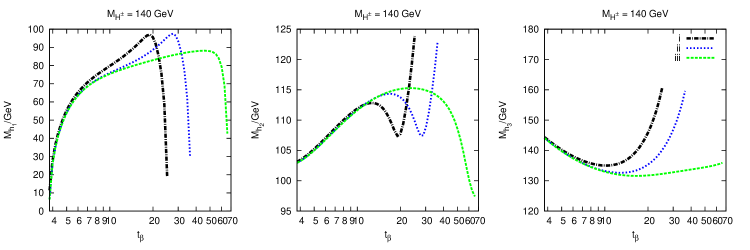
Figure 3: Predictions for the neutral Higgs masses, $M_{h_{1}}$, $M_{h_{2}}$, $M_{h_{3}}$, obtained using the effective bottom quark mass employed for the numerical analyses in this paper, (iii) $m_{b,{\rm eff}}=m_{b}^{\overline{\rm{DR}},SM}(m_{t}^{OS})/|1+\Delta m_{b}^{\rm FH}|$ in comparison with two other choices for the bottom mass, (i) $m_{b}^{\overline{\rm{MS}},SM}(m_{b})$ and (ii) $m_{b}^{\overline{\rm{DR}},SM}(m_{t}^{OS})$. The results are shown for the $\rm{CPX}$ scenario with $M_{H^{\pm}}=140\,\,\mathrm{GeV}$.

It is desirable to incorporate leading $\tan\beta$-enhanced contributions also into the calculation of the Higgs self-energies. A direct application of the effective Lagrangian of eq. (37) within loop calculations is in general not possible, as it would spoil (among other things) the UV-finiteness of the theory. It is therefore convenient to absorb the leading $\tan\beta$-enhanced contributions into an effective bottom quark mass that is used everywhere in the calculation, although this procedure does not reproduce the decoupling properties of the effective Lagrangian of eq. (37) in the limit where $M_{H^{\pm}}\gg M_{Z}$. It has been shown in Refs. [85, 76] that the one-loop result with an appropriately chosen effective bottom quark mass in general approximates very well the result containing the diagrammatic two-loop contributions.

Because of the large value of $\mu$ in the CPX scenario, contributions from the bottom / sbottom sector can be important already for moderate values of $\tan\beta$. We use in the following an effective bottom quark mass that is defined as

$$m_{b,{\rm eff}}=\frac{m_{b}^{\overline{\rm{DR}},SM}(m_{t}^{OS})}{|1+\Delta m_{b}^{\rm FH}|},$$ (51)

where ‘$\overline{\rm{DR}}$’ or ‘$OS$’ indicates the renormalisation scheme in which the mass is defined i.e. the $\overline{\rm{DR}}$ or $OS$ renormalisation scheme respectively, and ‘SM’ indicates that only the Standard Model contribution is included. $\Delta m_{b}^{\rm FH}$ is the $\Delta m_{b}$ correction calculated internally by FeynHiggs for use in its Higgs decays and Higgs production cross sections.

Since in the CPX scenario $|1+\Delta m_{b}|>1$, the incorporation of the $\tan\beta$-enhanced $\Delta m_{b}$ corrections leads to a reduction of the numerical value of $m_{b,{\rm eff}}$ in this scenario and thus to numerically more stable results. This is illustrated in Fig. 3, where the results for the neutral Higgs masses obtained using the effective bottom quark mass defined in eq. (51) are compared with the predictions arising from choosing $m_{b}^{\overline{\rm{MS}},SM}(m_{b})$ or $m_{b}^{\overline{\rm{DR}},SM}(m_{t}^{OS})$ for the bottom quark mass. For large values of $\tan\beta$, depending on the choice of the bottom mass, an onset of very large corrections from the bottom / sbottom sector is visible in the predictions for the Higgs masses. Since perturbative predictions are not reliable in the parameter region where these large corrections from the bottom / sbottom sector occur, we limit the numerical analyses in this paper to the region $\tan\beta<30$. (Without resummation of the $\tan\beta$-enhanced contributions as in eq. (51), the onset of very large corrections could already occur at lower values of $\tan\beta$.)

5 Conversion of parameters between on-shell and $\overline{\rm{DR}}$ renormalisation schemes

As mentioned above, higher-order contributions in the Higgs sector of the MSSM have been obtained using different approaches. The results implemented in the public code FeynHiggs [6, 7, 8, 9, 10] are based on the Feynman-diagrammatic approach employing the on-shell renormalisation scheme, while the results implemented in the public code CPsuperH [11, 12] are based on a renormalisation group improved effective potential calculation employing $\overline{\rm{DR}}$ renormalisation. As the parameters in the two renormalisation schemes are defined differently, a parameter conversion is necessary for a meaningful comparison of results obtained in the two schemes.

5.1 Parameter shifts

Since both schemes incorporate partial 2-loop contributions, a parameter conversion of the top/stop sector parameters (that enter at the 1-loop level), is required. In Refs. [77, 82] this issue has been discussed for the case where all the MSSM parameters are real. In the following we consider the general case of arbitrary complex parameters. We can obtain the leading terms at $\mathcal{O}(\alpha_{s})$ from considering loops involving gluons, gluinos, stops and tops as shown in Fig. 4. In order to obtain the leading terms at $\mathcal{O}(\alpha_{t})$, we must also consider loops involving neutralinos, charginos, Higgs bosons, Goldstone bosons, sbottoms and b-quarks, as shown in Fig. 5.

Figure 4: The diagrams used to calculate the shifts shown in eqs. (54) – (59), (which convert between $\overline{\rm{DR}}$ and on-shell parameters) at $\mathcal{O}(\alpha_{s})$. ($x=1,2,\,y=1,2,\ z=1,2$)

Figure 5: The diagrams used to calculate the shifts shown in eqs. (54) – (59) (which convert between $\overline{\rm{DR}}$ and on-shell parameters) at $\mathcal{O}(\alpha_{t})$. ($x=1,2,\,y=1,2,\ z=1,2,\ i=1,2,3,\ n=1,2,3,4$)

We label the difference between the parameters $p$ in the different renormalisation schemes by $\Delta p$, where

$$p^{\rm\overline{\rm{DR}}} = p^{\rm on-shell}+\Delta p(\mu_{\rm ren}).$$ (52)

Since the $\overline{\rm{DR}}$ parameters depend on the renormalisation scale $\mu_{\rm ren}$, the shift $\Delta p$ is also a function of $\mu_{\rm ren}$. The parameter shift $\Delta p$ is related to the counterterms by

$$\Delta p(\mu_{\rm ren}) =\delta p^{\rm on-shell}-\delta p^{\rm\overline{\rm{DR}}} =\delta p^{\rm on-shell}-\left[\delta p^{\rm on-shell}\right]^{\rm div},$$ (53)

where the superscript ‘div’ denotes that only terms proportional to $\frac{2}{4-D}-\gamma_{E}+\log(4\pi)$ are kept. Therefore this means that $\Delta p(\mu_{\rm ren})=\left[\delta p^{\rm on-shell}\right]^{\rm fin}$, where the superscript ‘fin’ denotes the finite pieces remaining once terms proportional to $\frac{2}{4-D}-\gamma_{E}+\log(4\pi)$ have been subtracted out.

For the stop sector, we can directly adapt the counterterms used in FeynHiggs in Ref. [110] (see App. B for the explicit form of the counterterms) to get the parameter shifts

$$\Delta M_{L}^{2} = -2m_{t}\Delta m_{t}+U_{11}^{*}U_{11}\Delta m^{2}_{\tilde{t}_{1}}+U_{21}^{*}U_{21}\Delta m^{2}_{\tilde{t}_{2}}+U_{11}^{*}U_{21}\Delta Y_{\tilde{t}}+U_{21}^{*}U_{11}\Delta Y^{*}_{\tilde{t}},$$ (54)

$$\Delta M_{\tilde{t}_{R}}^{2} = -2m_{t}\Delta m_{t}+U_{12}^{*}U_{12}\Delta m^{2}_{\tilde{t}_{1}}+U_{22}^{*}U_{22}\Delta m^{2}_{\tilde{t}_{2}}+U_{12}^{*}U_{22}\Delta Y_{\tilde{t}}+U_{22}^{*}U_{12}\Delta Y^{*}_{\tilde{t}},$$ (55)

$$\Delta A^{*}_{t} = e^{-i\phi_{A_{t}}}\left(\Delta\left|A_{t}\right|-i\left|A_{t}\right|\Delta\phi_{A_{t}}\right),$$ (56)

$$\Delta K_{t} = -\left(A_{t}^{*}-\mu\cot\beta\right)\Delta m_{t}+m_{t}\cot\beta\Delta\mu$$ (57)

$$+U_{11}^{*}U_{12}\Delta m^{2}_{\tilde{t}_{1}}+U_{21}^{*}U_{22}\Delta m^{2}_{\tilde{t}_{2}}+U_{11}^{*}U_{22}\Delta Y_{\tilde{t}}+U_{21}^{*}U_{12}\Delta Y^{*}_{\tilde{t}},$$

$$\Delta\left|A_{t}\right| = \frac{1}{m_{t}}{\rm Re}\left[e^{i\phi_{A_{t}}}\Delta K_{t}\right],$$ (58)

$$\Delta\phi_{A_{t}} = -\frac{1}{m_{t}\left|A_{t}\right|}{\rm Im}\left[e^{i\phi_{A_{t}}}\Delta K_{t}\right],$$ (59)

where

$$\Delta m_{t} = \frac{1}{2}{\rm Re}\left[m\left(\Sigma_{t}^{L}(m^{2})+\Sigma_{t}^{R}(m^{2})\right)+\Sigma_{t}^{l}(m^{2})+\Sigma_{t}^{r}(m^{2})\right]^{\rm fin},$$ (60)

$$\Delta m_{\tilde{t}_{1}}^{2} = {\rm Re}\left[\Sigma_{\tilde{t}_{11}}(m^{2}_{\tilde{t}_{1}})\right]^{\rm fin},$$ (61)

$$\Delta m_{\tilde{t}_{2}}^{2} = {\rm Re}\left[\Sigma_{\tilde{t}_{22}}(m^{2}_{\tilde{t}_{2}})\right]^{\rm fin},$$ (62)

$$\Delta Y_{\tilde{t}} = \frac{1}{2}\left[\widetilde{\rm Re}\Sigma_{\tilde{t}_{12}}(m^{2}_{\tilde{t}_{1}})+\widetilde{\rm Re}\Sigma_{\tilde{t}_{12}}(m^{2}_{\tilde{t}_{2}})\right]^{\rm fin},$$ (63)

and the components of the top self-energy are defined by $\Sigma(p)=\makebox[0.86108pt][l]{$p$}/\omega_{-}\Sigma^{L}(p^{2})+\makebox[0.86108pt][l]{$p$}/\omega_{+}\Sigma^{R}(p^{2})+\omega_{-}\Sigma^{l}(p^{2})+\omega_{+}\Sigma^{r}(p^{2})$, and ${\rm\widetilde{Re}}$ indicates that the imaginary parts of the loop integrals are discarded.

In the following we will define the $\overline{\rm{DR}}$ parameters at the scale $\mu_{\rm ren}=\sqrt{M_{\rm SUSY}^{2}+m_{t}^{2}}=:M_{S}$, see Ref. [11] and the discussion in Ref. [77]. We evaluate the strong coupling constant at the scale of the top mass, $\alpha_{s}(m_{t}^{2})$. Since the two-loop corrections of $\mathcal{O}(\alpha_{t}\alpha_{s})$ and $\mathcal{O}(\alpha_{t}^{2})$ implemented in FeynHiggs have been obtained using a Yukawa approximation (the corresponding contributions are implemented in CPsuperH only to leading logarithmic accuracy), we employ the same kind of approximation to derive the parameter conversions at $\mathcal{O}(\alpha_{s})$ and $\mathcal{O}(\alpha_{t})$. In particular, we neglect the D-terms in the stop mass matrix (i.e., the terms proportional to $M_{Z}^{2}$), the D-terms and the b-quark mass in the sbottom mass matrix, and we neglect terms proportional to $M_{1}$, $M_{2}$, $M_{Z}$, $M_{W}$ in the neutralino and chargino mass matrices. In addition, we make the approximation $M_{H\pm}=M_{A}$ when deriving the parameter shifts.

For the evaluation of the parameter shifts at $\mathcal{O}(\alpha_{t})$ we also need to consider a shift to the Higgsino mass parameter $\mu$, since FeynHiggs takes $\mu^{\overline{\rm{DR}}}(m_{t})$ as input while CPsuperH takes $\mu^{\overline{\rm{DR}}}(M_{S})$ as input. Therefore we use the relation

$$\mu(m_{t}) = \mu(M_{S})+\frac{3\alpha_{t}}{8\pi}\mu\log\left(\frac{m_{t}^{2}}{M_{S}^{2}}\right).$$ (64)

The difference between using $\overline{\rm{DR}}$ or on-shell quantities as input to the shifts $\Delta p$ is of higher order.

5.2 Simple approximation of parameter shifts

It is useful to find a simple approximation for the $\mathcal{O}(\alpha_{s})$ contribution to the parameter shifts $\Delta p$. It turns out that the shifts in $M_{L}$ and $M_{\tilde{t}_{R}}$ in general are less numerically significant than the shifts in $A_{t}$. Therefore we investigate an approximate treatment in which the shifts in $M_{L}$ and $M_{\tilde{t}_{R}}$ are neglected. Furthermore, since we have neglected the D-terms in the stop mass matrix and use $M_{\rm SUSY}^{\overline{\rm{DR}}}(M_{S})=M^{\overline{\rm{DR}}}_{L}(M_{S})=M^{\overline{\rm{DR}}}_{\tilde{t}_{R}}(M_{S})$, the stop mixing matrix defined in eq. (12) has the simple form

$${\mathbf{U}}_{\tilde{q}}=\frac{1}{\sqrt{2}}\left(\begin{array}[]{cc}1&-e^{-i\phi_{X_{t}}}\\ e^{i\phi_{X_{t}}}&1\end{array}\right).$$ (67)

Accordingly, the relation between $|X_{t}^{\rm on-shell}|$ and $|X_{t}^{\overline{\rm{DR}}}(M_{S})|$ simplifies to

$$|X_{t}^{\rm on-shell}| = |X_{t}^{\overline{\rm{DR}}}|\left(1+\frac{\Delta m_{t}}{m_{t}}\right)-\frac{1}{2m_{t}}\left(\Delta m^{2}_{\tilde{t}_{2}}-\Delta m^{2}_{\tilde{t}_{1}}\right),$$ (68)

where

$$\Delta m_{t} = \frac{\alpha_{s}}{6\pi m_{t}}\left[g_{1}^{t}+g_{2}^{t}+m_{t}^{2}\left(6\log\frac{m_{t}^{2}}{\mu^{2}_{\rm ren}}-10\right)+2m_{\tilde{g}}^{2}\left(\log\frac{m_{\tilde{g}}^{2}}{\mu^{2}_{\rm ren}}-1\right)\right],$$ (69)

$$\Delta m^{2}_{\tilde{t}_{1}}-\Delta m^{2}_{\tilde{t}_{2}} = \frac{2\alpha_{s}}{3\pi}\left(g_{1}^{\tilde{t}}-g_{2}^{\tilde{t}}\right),$$ (70)

$$g_{i}^{t} = -m_{\tilde{t}_{i}}^{2}\left(\log\frac{m_{\tilde{t}_{i}}^{2}}{\mu^{2}_{\rm ren}}-1\right)+f_{i}{\rm Re}\left[\mathcal{B}_{0}[m_{t}^{2},m_{\tilde{g}}^{2},m_{\tilde{t}_{i}}^{2}]\right],$$ (71)

$$g_{i}^{\tilde{t}} = 2m_{\tilde{t}_{i}}^{2}\left(\log\frac{m_{\tilde{t}_{i}}^{2}}{\mu^{2}_{\rm ren}}-2\right)-f_{i}{\rm Re}\left[\mathcal{B}_{0}[m_{\tilde{t}_{i}}^{2},m_{\tilde{g}}^{2},m_{t}^{2}]\right],$$ (72)

$$f_{i} = m_{\tilde{g}}^{2}+m_{t}^{2}-m_{\tilde{t}_{i}}^{2}-(-1)^{i}2m_{\tilde{g}}m_{t}\cos(\phi_{M_{3}}-\phi_{X_{t}}),$$ (73)

and $\mathcal{B}_{0}=\left[B_{0}\right]^{\rm fin}$, with the scalar integral $B_{0}$ defined as

$$B_{0}(p_{1}^{2},m_{0}^{2},m_{1}^{2}) = \frac{(2\pi\mu)^{4-D}}{i\pi^{2}}\int d^{D}q\frac{1}{(q^{2}-m_{0}^{2}+i\epsilon)((q+p_{1})^{2}-m_{1}^{2}+i\epsilon)}.$$ (74)

5.3 Numerical examples in the $\overline{\rm{CPX}}$ scheme

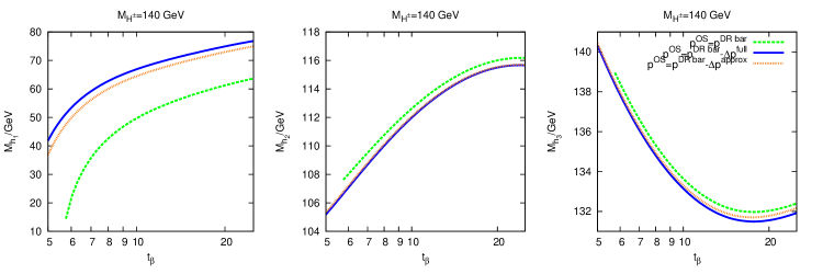
Figure 6: Impact of parameter conversions on the neutral Higgs masses $M_{h_{1}}$, $M_{h_{2}}$, $M_{h_{3}}$. The predictions for the Higgs masses, evaluated with the program FeynHiggs, are shown as a function of $\tan\beta$ in the $\overline{\rm{CPX}}$ scenario. Green (dashed): Result where the numerical values of the input parameters $A_{t}^{\overline{\rm{DR}}}(M_{S})$, $M_{L}^{\overline{\rm{DR}}}(M_{S})$, $M_{\tilde{t}_{R}}^{\overline{\rm{DR}}}(M_{S})$ are directly inserted into FeynHiggs without a parameter conversion (i.e., $\Delta p=0$). Blue (solid): Output of FeynHiggs if on-shell values of the parameters are inserted that are obtained from the ${\overline{\rm{DR}}}$ input values using the full expressions for $\Delta p$ given in eqs. (54)–(59) at $\mathcal{O}(\alpha_{s})$. Orange (dotted): Output of FeynHiggs if the parameter conversion is calculated using the approximation described in Sect. 5.2.

In Fig. 6 we investigate the impact of the $\mathcal{O}(\alpha_{s})$ parameter conversions on the predictions for the neutral Higgs masses $M_{h_{1}}$, $M_{h_{2}}$, $M_{h_{3}}$ (see Sect. 10.3 for a discussion of the $\mathcal{O}(\alpha_{t})$ terms). We compare the case where the numerical values of the input parameters $A_{t}^{\overline{\rm{DR}}}(M_{S})$, $M_{L}^{\overline{\rm{DR}}}(M_{S})$, $M_{\tilde{t}_{R}}^{\overline{\rm{DR}}}(M_{S})$ in the $\overline{\rm{CPX}}$ scheme (for $M_{H^{\pm}}=140\,\,\mathrm{GeV}$) are directly inserted as input into the program FeynHiggs (in which the parameters are interpreted as on-shell quantities) with the case where a proper conversion of the ${\overline{\rm{DR}}}$ input values to on-shell parameters has been carried out at $\mathcal{O}(\alpha_{s})$ according to eqs. (54)–(59). One can see that the parameter shifts have a very large numerical impact on the prediction of the lightest Higgs mass of more than $20\,\,\mathrm{GeV}$ in the region of small $\tan\beta$, while the corresponding effects on the predictions for $M_{h_{2}}$ and $M_{h_{3}}$ are typically below the GeV level. The result for $M_{h_{1}}$ indicates the well-known fact that corrections of ${\cal O}(\alpha_{t}\alpha_{s})$ in the MSSM Higgs sector can be numerically very important. The numerical effects found here in the $\overline{\rm{CPX}}$ scenario are even larger than the corresponding shifts in the case of real parameters as discussed in Ref. [77]. As a consequence, it is obvious that a proper conversion of parameters at least for the prediction of the lightest Higgs mass is indispensable for a meaningful comparison of results obtained in different renormalisation schemes.

Also shown in Fig. 6 is the result obtained from employing the approximate parameter conversion as given in Sect. 5.2. One can see that the result for the approximate treatment is close to the one obtained with the full parameter conversion. This indicates that the main impact of the parameter conversion is indeed caused by the shift in the absolute value of the trilinear coupling $\Delta|A_{t}|$, as expected from the discussion above. From the expressions given in Sect. 5.2 one can furthermore see that there is a significant dependence on the phase $(\phi_{M_{3}}-\phi_{X_{t}})$ and that the gluino mass $|M_{3}|$ plays an important role. We will use the full $\mathcal{O}(\alpha_{s})$ parameter conversions throughout the rest of the paper. However, we note that this approximate parameter conversion can be useful in situations where the inclusion of the full $\mathcal{O}(\alpha_{s})$ parameter conversions is impractical.

5.4 Reparametrisation of $m_{t}$ in the neutral Higgs self-energies

The difference between parametrising the neutral Higgs self-energies in terms of the on-shell top mass and parametrising the neutral Higgs self-energies in terms of the $\overline{\rm{MS}}$ top mass is formally a three-loop effect. Previously, we have chosen to use an on-shell top mass. We shall now investigate the numerical effect of parametrising in terms of the $\overline{\rm{MS}}$ top mass $\overline{m}_{t}:=m_{t}^{\overline{\rm{MS}},SM}(m_{t})$. In order to simplify the following discussion, we shall assume no resummation of $\tan\beta$-enhanced terms.

So far, we have been using neutral Higgs self-energies expressed in terms of the on-shell top mass:

$$\hat{\Sigma}(m_{t}^{OS}) = \hat{\Sigma}^{(1)}_{\rm Yuk}(m_{t}^{OS})+\hat{\Sigma}^{(1)}_{\rm non-Yuk}(m_{t}^{OS})+\hat{\Sigma}^{(2)}_{\rm Yuk}(m_{t}^{OS})+h.o.t.$$ (75)

where ‘$h.o.t.$’ stands for ‘higher order terms’, and the on-shell top mass and the $\overline{\rm{MS}}$ top mass are related through

$$\overline{m}_{t} = m_{t}^{OS}+\alpha_{s}x$$

$$x = -\frac{4}{3\pi}m_{t}$$ (76)

The difference between using an on-shell top mass and the $\overline{\rm{MS}}$ top mass in $x$ is not important, since it will affect the calculation only at the 4-loop level. (We shall use $m_{t}^{OS}$).

We substitute for $m_{t}^{OS}$ in $\hat{\Sigma}(m_{t}^{OS})$

$$\hat{\Sigma}(m_{t}^{OS}) = \hat{\Sigma}^{(1)}_{\rm Yuk}(\overline{m}_{t}-\alpha_{s}x)+\hat{\Sigma}^{(1)}_{\rm non-Yuk}(\overline{m}_{t}-\alpha_{s}x)+\hat{\Sigma}^{(2)}_{\rm Yuk}(\overline{m}_{t}-\alpha_{s}x)+...$$ (77)

and perform an expansion around $x=0$, keeping terms up to $\mathcal{O}(\alpha_{t}\alpha_{s})$

$$\hat{\Sigma}(m_{t}^{OS}) = \hat{\Sigma}^{(1)}_{\rm Yuk}(\overline{m}_{t})-\alpha_{s}x\hat{\Sigma}^{(1)^{\prime}}_{\rm Yuk}(\overline{m}_{t})+\hat{\Sigma}^{(1)}_{\rm non-Yuk}(\overline{m}_{t})+\hat{\Sigma}^{(2)}_{\rm Yuk}(\overline{m}_{t})+...$$ (78)

The reparametrisation according to eq. (76) has generated an additional term $-\alpha_{s}x\hat{\Sigma}^{(1)^{\prime}}_{\rm Yuk}(m)$, which is of two-loop order. In order to calculate this additional term, we require the explicit expressions for the leading 1-loop Yukawa corrections to the neutral Higgs self-energies, which we give explicitly in eq. (105)–eq. (110) below.

We first substitute for the stop masses their expressions in terms of the top mass and the soft SUSY-breaking parameters, in order to ensure that the top mass dependence is explicit everywhere. We employ here the Yukawa approximation, i.e. eq. (5) simplifies to

$$m_{\tilde{q}_{1,2}}^{2} = m_{q}^{2}+\frac{1}{2}\Bigl{[}M_{L}^{2}+M_{\tilde{q}_{R}}^{2}\mp\sqrt{[M_{L}^{2}-M_{\tilde{q}_{R}}^{2}]^{2}+4m_{q}^{2}|X_{q}|^{2}}~{}\Bigr{]}.$$ (79)

Then we make the substitution $m_{t}\to m_{t}-\alpha_{s}x$ and expand around $x=0$ to obtain terms at $\mathcal{O}({\alpha_{t}\alpha_{s}})$. We then edit the FeynHiggs code to include these additional terms and make use of the option in FeynHiggs where the tree level stop sector parameters are calculated using $\overline{m}_{t}$ rather than $m_{t}^{OS}$.

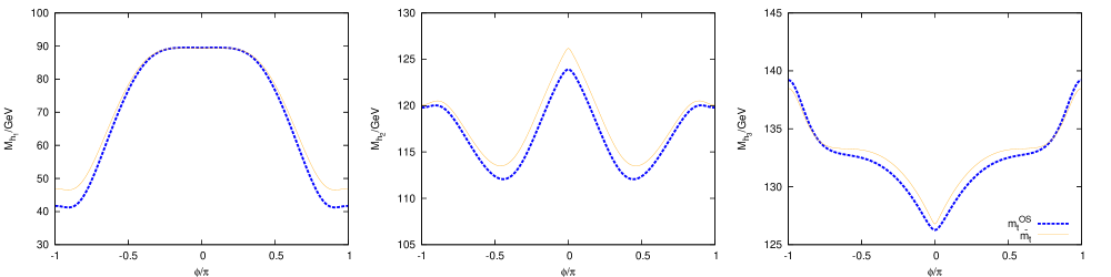
Figure 7: Neutral Higgs masses in the $CPX$ scenario at $\tan\beta=11$ and $M_{H^{\pm}}=140\,\,\mathrm{GeV}$ as function of phase $\phi=\phi_{A_{t}}=\phi_{M_{3}}$. Blue (dashed): the Higgs self-energy calculation is parameterised in terms of $m_{t}^{OS}$, orange (solid): the calculation is parametrised in terms of $\overline{m}_{t}$.

5.4.1 Numerical results

Fig. 7 shows the neutral Higgs masses in the $CPX$ scenario at $\tan\beta=11$ and $M_{H^{\pm}}=140\,\,\mathrm{GeV}$ as function of phase $\phi=\phi_{A_{t}}=\phi_{M_{3}}$, with the Higgs self-energy calculation parameterised in terms of $m_{t}^{OS}$ (blue, dashed) and in terms of $\overline{m}_{t}$ (orange, solid). These results include the resummation of $\tan\beta$-enhanced terms. We can see that, even in the CP-conserving limit, parameterising the calculation in terms of $\overline{m}_{t}$ rather than $m_{t}^{OS}$ can increase the lightest Higgs mass by $5.3\,\,\mathrm{GeV}$. However, note that we will be interested in the maximally CP-violating case $\phi=\pi/2$, where we can see that the effect on $M_{h_{1}}$ is more modest: a $1.6\,\,\mathrm{GeV}$ absolute increase or a $2\%$ relative increase.

6 Higgs cascade decay

We use the general expression for 2-body neutral Higgs boson decays,

$$\Gamma(h_{a}\rightarrow h_{b}h_{c}) = \frac{\mathcal{S}\rho|\mathcal{M}|^{2}}{8\pi M_{h_{a}}^{2}},$$ (80)

where $\mathcal{M}$ is the matrix element.

For identical final state particles, $h_{b}=h_{c}$,

$$\rho = \frac{M_{h_{a}}}{2}\sqrt{1-\frac{4M_{h_{b}}^{2}}{M_{h_{a}}^{2}}},$$ (81)

and the symmetry factor $\mathcal{S}$ is $\frac{1}{2}$. For the case $h_{b}\neq h_{c}$,

$$\rho = \frac{1}{2M_{h_{a}}}\sqrt{M_{h_{a}}^{4}+M_{h_{b}}^{4}+M_{h_{c}}^{4}-2\left(M_{h_{a}}^{2}M_{h_{b}}^{2}+M_{h_{b}}^{2}M_{h_{c}}^{2}+M_{h_{c}}^{2}M_{h_{a}}^{2}\right)},$$ (82)

and the symmetry factor is 1.

Since the lowest order contribution involves only scalar particles, the tree level decay width has a very simple form. For example, the $h\to AA$ tree level decay width is given by

$$\Gamma^{\rm tree}(h\rightarrow AA) = \frac{\lambda_{hAA}^{\rm tree,2}}{32\pi m_{h_{a}}}\sqrt{1-\frac{4m_{A}^{2}}{m_{h}^{2}}},{\rm\,with\,}\lambda_{hAA}^{\rm tree}=-c_{2\beta}s_{\alpha+\beta}\frac{eM_{W}}{2c_{W}^{2}s_{W}}.$$ (83)

6.1 Calculation of the genuine $h_{i}\to h_{j}h_{k}$ vertex contributions

We calculate the full 1PI (one-particle irreducible) 1-loop vertex corrections to the $h_{i}\to h_{j}h_{k}$ decay width within the Feynman-diagrammatic approach, taking into account the phases of all supersymmetric parameters. $h_{i},h_{j},h_{k}$ are some combination of the tree level Higgs fields $h,H,A$. The programs FeynArts [119, 120, 121] and FormCalc [121, 122] are used to draw and evaluate the Feynman diagrams using dimensional reduction, and LoopTools [122] is used to evaluate the majority of the integrals. We use $m_{b}=m_{b}^{\overline{\rm{MS}},SM}(m_{t}^{OS})$ and a top mass of $m_{t}=m_{t}^{\overline{\rm{MS}},SM}(m_{t}^{OS})=m_{t}^{OS}/\left(1+\frac{4}{3\pi}\alpha_{s}(m_{t}^{OS})\right)$ in the $t,\tilde{t},b,\tilde{b}$ masses which enter the genuine vertex corrections in order to absorb some of the higher order SM QCD corrections. We use a unit CKM matrix and assume no squark generation mixing.

6.1.1 Leading corrections (Yukawa terms)

At low to moderate values of $\tan\beta$, the leading corrections to the $h_{i}\to h_{j}h_{k}$ vertex are the Yukawa terms from the $t,\tilde{t}$ sector. These arise from the diagrams shown in Fig. 8.

Figure 8: The leading vertex corrections to the decay $h_{i}\to h_{j}h_{k}$, involving $t/\tilde{t}$ loops. ($x,y,z$ = 1,2)

As a first step, we select only terms proportional to $m_{t}^{4}/(M^{3}_{W}s_{W}^{3})$ (‘Yukawa terms’) and perform the calculation at zero incoming momentum i.e. $\hat{\Sigma}_{ij}(p^{2}=0)$. In this way, we obtain compact analytical expressions for the leading corrections to the $h_{i}h_{j}h_{k}$ vertex. We find that there are no counterterms contributing to the $h_{i}h_{j}h_{k}$ vertex in this approximation.

Note that, for consistency, the stop masses $m_{\tilde{t}_{1}}$ and $m_{\tilde{t}_{2}}$ must also be calculated in the Yukawa approximation according to eq. (79). We therefore arrive at the following expressions for the leading Yukawa corrections in the $t/\tilde{t}$ sector, which we can express as corrections to an effective coupling $i\lambda^{\rm eff}=i\lambda^{\rm tree}+i\Delta\lambda^{\rm Yuk}$.

For vertices involving the CP-even tree-level Higgs bosons for the case $m_{\tilde{t}_{1}}\neq m_{\tilde{t}_{2}}$ (the expressions for $m_{\tilde{t}_{1}}=m_{\tilde{t}_{2}}$ are given in App. C):

$$\Delta\lambda^{\rm Yuk}_{\phi_{1}\phi_{1}\phi_{1}} = -\frac{3e^{3}m_{t}^{4}}{32\pi^{2}M_{W}^{3}s_{W}^{3}s_{\beta}^{3}}\frac{\mbox{Re}\,{\left[\mu X_{t}\right]}}{m_{\tilde{t}_{1}}^{2}-m_{\tilde{t}_{2}}^{2}}\left\{4m_{t}^{2}\left(\mbox{Re}\,{\left[\mu X_{t}\right]}\right)^{2}\mathcal{E}_{11122-11222}+3\mu\mu^{*}\mathcal{C}_{112-122}\right\},$$

$$\Delta\lambda^{\rm Yuk}_{\phi_{1}\phi_{1}\phi_{2}} = -\frac{3e^{3}m_{t}^{4}}{32\pi^{2}M_{W}^{3}s_{W}^{3}s_{\beta}^{3}}\frac{1}{m_{\tilde{t}_{1}}^{2}-m_{\tilde{t}_{2}}^{2}}\left\{\mu\mu^{*}\left(2\log\left(\frac{m_{\tilde{t}_{1}}}{m_{\tilde{t}_{2}}}\right)-3\mbox{Re}\,{\left[A_{t}^{*}X_{t}\right]}\mathcal{C}_{112-122}\right)\right.$$ (85)

$$-4m_{t}^{2}\left(\mbox{Re}\,{\left[\mu X_{t}\right]}\right)^{2}\left(\mathcal{D}_{1112-1222}+\mbox{Re}\,{\left[A_{t}^{*}X_{t}\right]}\mathcal{E}_{11122-11222}\right)$$

$$\left.+2\left(\mbox{Im}\,{\left[\mu X_{t}\right]}\right)^{2}\mathcal{C}_{112-122}\right\},$$

$$\Delta\lambda^{\rm Yuk}_{\phi_{1}\phi_{2}\phi_{2}} = \frac{3e^{3}m_{t}^{4}}{16\pi^{2}M_{W}^{3}s_{W}^{3}s_{\beta}^{5}}\frac{1}{m_{\tilde{t}_{1}}^{2}-m_{\tilde{t}_{2}}^{2}}\left\{2\mu\mu^{*}s_{\beta}c_{\beta}\log\left(\frac{m_{\tilde{t}_{1}}}{m_{\tilde{t}_{2}}}\right)\right.$$ (86)

$$-s_{\beta}^{2}\mbox{Re}\,{\left[\mu X_{t}\right]}\left(\frac{m_{t}^{2}}{m_{\tilde{t}_{1}}^{2}m_{\tilde{t}_{2}}^{2}}\left(m_{\tilde{t}_{1}}^{2}-m_{\tilde{t}_{2}}^{2}\right)-3\log\left(\frac{m_{\tilde{t}_{1}}}{m_{\tilde{t}_{2}}}\right)+\frac{3}{2}\mathcal{C}_{112-122}A_{t}A_{t}^{*}\ \right.$$

$$\left.+2m_{t}^{2}\mbox{Re}\,{\left[A_{t}^{*}X_{t}\right]}\left(2\mathcal{D}_{1112-1222}+\mathcal{E}_{11122-11222}\mbox{Re}\,{\left[A_{t}^{*}X_{t}\right]}\right)\right)$$

$$\left.-c_{\beta}s_{\beta}\left(\mbox{Im}\,{\left[\mu X_{t}\right]}\right)^{2}\mathcal{C}_{112-122}\right\},$$

$$\Delta\lambda^{\rm Yuk}_{\phi_{2}\phi_{2}\phi_{2}} = \frac{3e^{3}m_{t}^{4}}{16\pi^{2}M_{W}^{3}s_{W}^{3}s_{\beta}^{3}}\frac{1}{m_{\tilde{t}_{1}}^{2}-m_{\tilde{t}_{2}}^{2}}\left\{\left(m_{\tilde{t}_{1}}^{2}-m_{\tilde{t}_{2}}^{2}\right)\left(2-3\log\left(\frac{m_{\tilde{t}_{1}}m_{\tilde{t}_{2}}}{m_{t}^{2}}\right)\right)\right.$$ (87)

$$-3\log\left(\frac{m_{\tilde{t}_{1}}}{m_{\tilde{t}_{2}}}\right)\left(A_{t}A_{t}^{*}+\mbox{Re}\,{\left[A_{t}^{*}X_{t}\right]}\right)-\frac{m_{t}^{2}}{m_{\tilde{t}_{1}}^{2}m_{\tilde{t}_{2}}^{2}}\left(m_{\tilde{t}_{1}}^{4}-m_{\tilde{t}_{2}}^{4}\right)$$

$$+3\mbox{Re}\,{\left[A_{t}^{*}X_{t}\right]}\left(\frac{m_{t}^{2}}{m_{\tilde{t}_{1}}^{2}m_{\tilde{t}_{2}}^{2}}\left(m_{\tilde{t}_{1}}^{2}-m_{\tilde{t}_{2}}^{2}\right)+\frac{1}{2}\mathcal{C}_{112-122}A_{t}A_{t}^{*}\right.$$

$$\left.\left.+\frac{2}{3}m_{t}^{2}\mbox{Re}\,{\left[A_{t}^{*}X_{t}\right]}\left(3\mathcal{D}_{1112-1222}+\mathcal{E}_{11122-11222}\mbox{Re}\,{\left[A_{t}^{*}X_{t}\right]}\right)\right)\right\},$$

where

$$Y_{t} = A_{t}+t_{\beta}\mu^{*}$$ (88)

$$\mathcal{C}_{112-122} = C_{0}\left(0,0,0,m_{\tilde{t}_{1}}^{2},m_{\tilde{t}_{1}}^{2},m_{\tilde{t}_{2}}^{2}\right)-C_{0}\left(0,0,0,m_{\tilde{t}_{1}}^{2},m_{\tilde{t}_{2}}^{2},m_{\tilde{t}_{2}}^{2}\right)$$ (89)

$$= -2\left(\frac{1}{m_{\tilde{t}_{1}}^{2}-m_{\tilde{t}_{2}}^{2}}-\frac{\left(m_{\tilde{t}_{1}}^{2}+m_{\tilde{t}_{2}}^{2}\right)}{\left(m_{\tilde{t}_{1}}^{2}-m_{\tilde{t}_{2}}^{2}\right)^{2}}\log\left(\frac{m_{\tilde{t}_{1}}}{m_{\tilde{t}_{2}}}\right)\right),$$

$$\mathcal{D}_{1112-1222} = \text{D}_{0}\left(0,0,0,0,m_{\tilde{t}_{1}}^{2},m_{\tilde{t}_{1}}^{2},m_{\tilde{t}_{1}}^{2},m_{\tilde{t}_{2}}^{2}\right)-\text{D}_{0}\left(0,0,0,0,m_{\tilde{t}_{1}}^{2},m_{\tilde{t}_{2}}^{2},m_{\tilde{t}_{2}}^{2},m_{\tilde{t}_{2}}^{2}\right)$$ (90)

$$= -\frac{1}{2\left(m_{\tilde{t}_{1}}^{2}-m_{\tilde{t}_{2}}^{2}\right)}\left(\frac{m_{\tilde{t}_{1}}^{2}+m_{\tilde{t}_{2}}^{2}}{m_{\tilde{t}_{1}}^{2}m_{\tilde{t}_{2}}^{2}}-\frac{4}{m_{\tilde{t}_{1}}^{2}-m_{\tilde{t}_{2}}^{2}}\log\left(\frac{m_{\tilde{t}_{1}}}{m_{\tilde{t}_{2}}}\right)\right),$$

$$\mathcal{E}_{11122-11222} = \text{E}_{0}\left(0,0,0,0,0,m_{\tilde{t}_{1}}^{2},m_{\tilde{t}_{1}}^{2},m_{\tilde{t}_{1}}^{2},m_{\tilde{t}_{2}}^{2},m_{\tilde{t}_{2}}^{2}\right)$$ (91)

$$- \text{E}_{0}\left(0,0,0,0,0,m_{\tilde{t}_{1}}^{2},m_{\tilde{t}_{1}}^{2},m_{\tilde{t}_{2}}^{2},m_{\tilde{t}_{2}}^{2},m_{\tilde{t}_{2}}^{2}\right)$$

$$= \frac{1}{2}\left(\frac{1}{m_{\tilde{t}_{1}}^{2}m_{\tilde{t}_{2}}^{2}\left(m_{\tilde{t}_{1}}^{2}-m_{\tilde{t}_{2}}^{2}\right)}\right.$$

$$+ \left.\frac{12}{\left(m_{\tilde{t}_{1}}^{2}-m_{\tilde{t}_{2}}^{2}\right)^{3}}\left(1-\frac{\left(m_{\tilde{t}_{1}}^{2}+m_{\tilde{t}_{2}}^{2}\right)}{\left(m_{\tilde{t}_{1}}^{2}-m_{\tilde{t}_{2}}^{2}\right)}\log\left(\frac{m_{\tilde{t}_{1}}}{m_{\tilde{t}_{2}}}\right)\right)\right),$$

and $m_{\tilde{q}_{1,2}}^{2}$ are the stop masses in the Yukawa approximation, as given by eq. (79). $\mathcal{C}_{112-122}$, $\mathcal{D}_{1112-1222}$ and $\mathcal{E}_{11122-11222}$ are functions of $C_{0}$, $D_{0}$ and $E_{0}$ scalar integrals, respectively. Since we are describing a process with 3 external legs, $D_{0}$ and $E_{0}$ do not appear explicitly in the Feynman diagrams. However, these functions are very useful for simplifying the vertex expressions.

The 1-loop corrections to a $h_{i}h_{j}h_{k}$ vertex involving at least one CP-odd eigenstate (again, for $m_{\tilde{t}_{1}}\neq m_{\tilde{t}_{2}}$) are given by

$$\Delta\lambda^{\rm Yuk}_{\phi_{1}\phi_{1}A} = \frac{3e^{3}m_{t}^{4}}{32\pi^{2}M_{W}^{3}s_{W}^{3}s_{\beta}^{4}}\frac{\mbox{Im}\,{\left[\mu X_{t}\right]}}{m_{\tilde{t}_{1}}^{2}-m_{\tilde{t}_{2}}^{2}}\left\{\right.$$ (92)

$$\left.\left(\mu\mu^{*}-2c_{\beta}s_{\beta}\mbox{Re}\,{\left[\mu X_{t}\right]}\right)\mathcal{C}_{112-122}+4m_{t}^{2}\left(\mbox{Re}\,{\left[\mu X_{t}\right]}\right)^{2}\mathcal{E}_{11122-11222}\right\},$$

$$\Delta\lambda^{\rm Yuk}_{\phi_{1}\phi_{2}A} = -\frac{3e^{3}m_{t}^{4}}{32\pi^{2}M_{W}^{3}s_{W}^{3}s_{\beta}^{4}}\frac{\mbox{Im}\,{\left[\mu X_{t}\right]}}{m_{\tilde{t}_{1}}^{2}-m_{\tilde{t}_{2}}^{2}}\left\{+2c_{\beta}s_{\beta}\log\left(\frac{m_{\tilde{t}_{1}}}{m_{\tilde{t}_{2}}}\right)\right.$$ (93)

$$+\left(2\mbox{Re}\,{\left[\mu A_{t}\right]}-c_{\beta}s_{\beta}\left(\mu\mu^{*}+A_{t}A_{t}^{*}\right)\right)\mathcal{C}_{112-122}$$

$$\left.+4m_{t}^{2}\mbox{Re}\,{\left[\mu X_{t}\right]}\left(\mathcal{D}_{1112-1222}+\mbox{Re}\,{\left[A_{t}^{*}X_{t}\right]}\mathcal{E}_{11122-11222}\right)\right\},$$

$$\Delta\lambda^{\rm Yuk}_{\phi_{2}\phi_{2}A} = -\frac{3e^{3}m_{t}^{4}}{32\pi^{2}M_{W}^{3}s_{W}^{3}s_{\beta}^{4}}\frac{\mbox{Im}\,{\left[\mu X_{t}\right]}}{m_{\tilde{t}_{1}}^{2}-m_{\tilde{t}_{2}}^{2}}\left\{-2\frac{m_{t}^{2}}{m_{\tilde{t}_{1}}^{2}m_{\tilde{t}_{2}}^{2}}\left(m_{\tilde{t}_{1}}^{2}-m_{\tilde{t}_{2}}^{2}\right)\right.$$ (94)

$$+2\left(2s_{\beta}^{2}+1\right)\log\left(\frac{m_{\tilde{t}_{1}}}{m_{\tilde{t}_{2}}}\right)-\left(2s_{\beta}^{2}\mbox{Re}\,{\left[A_{t}^{*}X_{t}\right]}+A_{t}A_{t}^{*}\right)\mathcal{C}_{112-122}$$

$$\left.-4m_{t}^{2}\mbox{Re}\,{\left[A_{t}^{*}X_{t}\right]}\left(2\mathcal{D}_{1112-1222}+\mbox{Re}\,{\left[A_{t}^{*}X_{t}\right]}\mathcal{E}_{11122-11222}\right)\right\},$$

$$\Delta\lambda^{\rm Yuk}_{\phi_{1}AA} = \frac{3e^{3}m_{t}^{4}}{32\pi^{2}M_{W}^{3}s_{W}^{3}s_{\beta}^{5}}\frac{1}{m_{\tilde{t}_{1}}^{2}-m_{\tilde{t}_{2}}^{2}}\left\{c^{2}_{\beta}s^{2}_{\beta}\mbox{Re}\,{\left[\mu X_{t}\right]}\left(2\log\left(\frac{m_{\tilde{t}_{1}}}{m_{\tilde{t}_{2}}}\right)-Y_{t}Y_{t}^{*}\mathcal{C}_{112-122}\right)\right.$$ (95)

$$\left.+2\left(\mbox{Im}\,{\left[\mu X_{t}\right]}\right)^{2}\left(c_{\beta}s_{\beta}\mathcal{C}_{112-122}-2m_{t}^{2}\mbox{Re}\,{\left[\mu X_{t}\right]}\mathcal{E}_{11122-11222}\right)\right\},$$

$$\Delta\lambda^{\rm Yuk}_{\phi_{2}AA} = \frac{3e^{3}m_{t}^{4}}{32\pi^{2}M_{W}^{3}s_{W}^{3}s_{\beta}^{5}}\frac{1}{m_{\tilde{t}_{1}}^{2}-m_{\tilde{t}_{2}}^{2}}\left\{s_{\beta}^{2}c_{\beta}^{2}\left(-2\left(m_{\tilde{t}_{1}}^{2}-m_{\tilde{t}_{2}}^{2}\right)\log\left(\frac{m_{\tilde{t}_{1}}m_{\tilde{t}_{2}}}{m_{t}^{2}}\right)\right.\right.$$

$$\left.-2\left(\mbox{Re}\,{\left[A_{t}^{*}X_{t}\right]}+Y_{t}Y_{t}^{*}\right)\log\left(\frac{m_{\tilde{t}_{1}}}{m_{\tilde{t}_{2}}}\right)+Y_{t}Y_{t}^{*}\mbox{Re}\,{\left[A_{t}^{*}X_{t}\right]}\mathcal{C}_{112-122}\right)$$

$$\left.+2\left(\mbox{Im}\,{\left[\mu X_{t}\right]}\right)^{2}\left(s_{\beta}^{2}\mathcal{C}_{112-122}+2m_{t}^{2}\left(\mathcal{D}_{1112-1222}+\mbox{Re}\,{\left[A_{t}^{*}X_{t}\right]}\mathcal{E}_{11122-11222}\right)\right)\right\},$$

$$\Delta\lambda^{\rm Yuk}_{AAA} = -\frac{3e^{3}m_{t}^{4}}{32\pi^{2}M_{W}^{3}s_{W}^{3}s_{\beta}^{6}}\frac{\left(\mbox{Im}\,{\left[\mu X_{t}\right]}\right)^{2}}{m_{\tilde{t}_{1}}^{2}-m_{\tilde{t}_{2}}^{2}}\left\{3c_{\beta}^{2}s_{\beta}^{2}\left(2\log\left(\frac{m_{\tilde{t}_{1}}}{m_{\tilde{t}_{2}}}\right)-Y_{t}Y_{t}^{*}\mathcal{C}_{112-122}\right)\right.$$ (97)

$$\left.-4m_{t}^{2}\left(\mbox{Im}\,{\left[\mu X_{t}\right]}\right)^{2}\mathcal{E}_{11122-11222}\right\}.$$

These compact, momentum independent expressions have the advantage that they are extremely easy to implement into a computer code. In this form, we are also able to see that, despite including the effect of complex phases, these corrections are themselves entirely real.

In order to convert these corrections to the $h,H,A$ basis, we use the mixing matrix from eq. (2). For example, $\lambda_{hAA}^{\rm eff}=\lambda_{hAA}^{\rm tree}-s_{\alpha}\Delta\lambda_{\phi_{1}AA}^{\rm Yuk}+c_{\alpha}\Delta\lambda_{\phi_{2}AA}^{\rm Yuk}$.

In the MSSM with real parameters and $m_{\tilde{t}_{1}}\neq m_{\tilde{t}_{2}}$, these corrections reduce to the form (here we drop the subscripts on $\mathcal{C}_{112-122},\mathcal{D}_{1112-1222},\mathcal{E}_{11122-11222}$ for brevity)

$$\Delta\lambda^{\rm Yuk,CPC}_{\phi_{1}\phi_{1}\phi_{1}} = -\frac{3e^{3}m_{t}^{4}}{32\pi^{2}M_{W}^{3}s_{W}^{3}s_{\beta}^{3}}\frac{\mu^{3}X_{t}}{m_{\tilde{t}_{1}}^{2}-m_{\tilde{t}_{2}}^{2}}\left\{4m_{t}^{2}X_{t}^{2}\mathcal{E}+3\mathcal{C}\right\},$$

$$\Delta\lambda^{\rm Yuk,CPC}_{\phi_{1}\phi_{1}\phi_{2}} = -\frac{3e^{3}m_{t}^{4}}{32\pi^{2}M_{W}^{3}s_{W}^{3}s_{\beta}^{3}}\frac{\mu^{2}}{m_{\tilde{t}_{1}}^{2}-m_{\tilde{t}_{2}}^{2}}\left\{2\log\left(\frac{m_{\tilde{t}_{1}}}{m_{\tilde{t}_{2}}}\right)-3A_{t}X_{t}\mathcal{C}-4m_{t}^{2}X_{t}^{2}\left(\mathcal{D}+A_{t}X_{t}\mathcal{E}\right)\right\},$$

$$\Delta\lambda^{\rm Yuk,CPC}_{\phi_{1}\phi_{2}\phi_{2}} = \frac{3e^{3}m_{t}^{4}}{32\pi^{2}M_{W}^{3}s_{W}^{3}s_{\beta}^{3}}\frac{2\mu}{m_{\tilde{t}_{1}}^{2}-m_{\tilde{t}_{2}}^{2}}\left\{(2A_{t}+X_{t})\log\left(\frac{m_{\tilde{t}_{1}}}{m_{\tilde{t}_{2}}}\right)\right.$$

$$-\frac{X_{t}m_{t}^{2}}{m_{\tilde{t}_{1}}^{2}m_{\tilde{t}_{2}}^{2}}\left(m_{\tilde{t}_{1}}^{2}-m_{\tilde{t}_{2}}^{2}\right)-\frac{3}{2}X_{t}A_{t}^{2}\mathcal{C}\ \left.-2m_{t}^{2}A_{t}X_{t}^{2}\left(2\mathcal{D}+A_{t}X_{t}\mathcal{E}\right)\right\},$$

$$\Delta\lambda^{\rm Yuk,CPC}_{\phi_{2}\phi_{2}\phi_{2}} = \frac{3e^{3}m_{t}^{4}}{32\pi^{2}M_{W}^{3}s_{W}^{3}s_{\beta}^{3}}\frac{2}{m_{\tilde{t}_{1}}^{2}-m_{\tilde{t}_{2}}^{2}}\left\{\left(m_{\tilde{t}_{1}}^{2}-m_{\tilde{t}_{2}}^{2}\right)\left(2-3\log\left(\frac{m_{\tilde{t}_{1}}m_{\tilde{t}_{2}}}{m_{t}^{2}}\right)\right)\right.$$

$$-3\log\left(\frac{m_{\tilde{t}_{1}}}{m_{\tilde{t}_{2}}}\right)A_{t}\left(A_{t}+X_{t}\right)-\frac{m_{t}^{2}}{m_{\tilde{t}_{1}}^{2}m_{\tilde{t}_{2}}^{2}}\left(m_{\tilde{t}_{1}}^{4}-m_{\tilde{t}_{2}}^{4}\right)$$

$$+3A_{t}X_{t}\left(\frac{m_{t}^{2}}{m_{\tilde{t}_{1}}^{2}m_{\tilde{t}_{2}}^{2}}\left(m_{\tilde{t}_{1}}^{2}-m_{\tilde{t}_{2}}^{2}\right)+\frac{1}{2}A_{t}^{2}\mathcal{C}\left.+\frac{2}{3}m_{t}^{2}A_{t}X_{t}\left(3\mathcal{D}+A_{t}X_{t}\mathcal{E}\right)\right)\right\},$$

$$\Delta\lambda^{\rm Yuk,CPC}_{\phi_{1}AA} = \frac{3e^{3}m_{t}^{4}}{32\pi^{2}M_{W}^{3}s_{W}^{3}s_{\beta}^{3}}\frac{c^{2}_{\beta}}{m_{\tilde{t}_{1}}^{2}-m_{\tilde{t}_{2}}^{2}}\left\{\mu X_{t}\left(2\log\left(\frac{m_{\tilde{t}_{1}}}{m_{\tilde{t}_{2}}}\right)-Y_{t}^{2}\mathcal{C}\right)\right\},$$ (102)

$$\Delta\lambda^{\rm Yuk,CPC}_{\phi_{2}AA} = \frac{3e^{3}m_{t}^{4}}{32\pi^{2}M_{W}^{3}s_{W}^{3}s_{\beta}^{3}}\frac{c_{\beta}^{2}}{m_{\tilde{t}_{1}}^{2}-m_{\tilde{t}_{2}}^{2}}\left\{-2\left(m_{\tilde{t}_{1}}^{2}-m_{\tilde{t}_{2}}^{2}\right)\log\left(\frac{m_{\tilde{t}_{1}}m_{\tilde{t}_{2}}}{m_{t}^{2}}\right)\right.$$

$$\left.-2\left(A_{t}X_{t}+Y_{t}^{2}\right)\log\left(\frac{m_{\tilde{t}_{1}}}{m_{\tilde{t}_{2}}}\right)+Y_{t}^{2}A_{t}X_{t}\mathcal{C}\right\}$$

and $\Delta\lambda^{\rm Yuk,CPC}_{\phi_{1}\phi_{1}A}=\Delta\lambda^{\rm Yuk,CPC}_{\phi_{1}\phi_{2}A}=\Delta\lambda^{\rm Yuk,CPC}_{\phi_{2}\phi_{2}A}=\Delta\lambda^{\rm Yuk,CPC}_{AAA}=0$. These expressions correspond exactly to the results for the leading Yukawa corrections to the triple Higgs vertex in the MSSM with real parameters published in Ref. [15].

For completeness, we also give the leading Yukawa corrections to the neutral Higgs self-energies in the complex MSSM, which we used when investigating the effect of reparametrising the Higgs self-energies in terms of the $\overline{\rm{MS}}$ top mass, as described in Sect. 5.4. These expressions can be found by considering diagrams involving $t,\tilde{t},b,\tilde{b}$ loops only and selecting those terms proportional to $m^{2}_{t}/M^{2}_{W}$ (‘Yukawa terms’). The resulting corrections will be finite and proportional to $m_{t}^{4}$. As before, the renormalisation constants $\delta t_{\beta}$, $\delta M_{W}^{2}$, $\delta M_{Z}^{2}$ and $\delta Z_{ij}$, are all zero in this approximation and the incoming momentum is taken to be zero. These expressions also involve the Higgs tadpoles and the charged Higgs self-energy (since $M_{H^{\pm}}$ is the input parameter rather than $M_{A}$), which is also taken at zero incoming momentum, such that

$$\delta M_{H^{\pm}}^{2} = \Sigma_{H^{-}H^{+}}\left(0\right).$$ (104)

The leading corrections to the renormalised neutral Higgs energies in the Yukawa approximation for $m_{\tilde{t}_{1}}\neq m_{\tilde{t}_{2}}$ are thus given by [109]:

$$\hat{\Sigma}^{(1)\phi_{1}\phi_{1}}_{\rm Yuk} = \frac{3e^{2}m_{t}^{4}}{16\pi^{2}M_{W}^{2}s_{W}^{2}s_{\beta}^{2}}\left(\frac{\left(\mbox{Re}\,{\left[\mu X_{t}\right]}\right)^{2}}{m_{\tilde{t}_{1}}^{2}-m_{\tilde{t}_{2}}^{2}}\mathcal{C}_{112-122}+\mu\mu^{*}\frac{\mathcal{C}_{12L}}{2}\right),$$ (105)

$$\hat{\Sigma}^{(1)\phi_{1}\phi_{2}}_{\rm Yuk} = -\frac{3e^{2}m_{t}^{4}}{16\pi^{2}M_{W}^{2}s_{W}^{2}s_{\beta}^{2}}\left(\frac{\mu\mu^{*}}{t_{\beta}}\frac{\mathcal{C}_{12L}}{2}\right.$$ (106)

$$\left.+\frac{\mbox{Re}\,{\left[\mu X_{t}\right]}}{m_{\tilde{t}_{1}}^{2}-m_{\tilde{t}_{2}}^{2}}\left(\mbox{Re}\,{\left[A_{t}^{*}X_{t}\right]}\mathcal{C}_{112-122}-2\log\left(\frac{m_{\tilde{t}_{1}}}{m_{\tilde{t}_{2}}}\right)\right)\right),$$

$$\hat{\Sigma}^{(1)\phi_{2}\phi_{2}}_{\rm Yuk} = -\frac{3e^{2}m_{t}^{4}}{16\pi^{2}M_{W}^{2}s_{W}^{2}s_{\beta}^{2}}\left(2\log\left(\frac{m_{\tilde{t}_{1}}m_{\tilde{t}_{2}}}{m_{t}^{2}}\right)-\frac{\mu\mu^{*}}{t_{\beta}^{2}}\frac{\mathcal{C}_{12L}}{2}\right.$$ (107)

$$\left.+\frac{\mbox{Re}\,{\left[A_{t}^{*}X_{t}\right]}}{m_{\tilde{t}_{1}}^{2}-m_{\tilde{t}_{2}}^{2}}\left(4\log\left(\frac{m_{\tilde{t}_{1}}}{m_{\tilde{t}_{2}}}\right)-\mbox{Re}\,{\left[A_{t}^{*}X_{t}\right]}\mathcal{C}_{112-122}\right)\right),$$

$$\hat{\Sigma}^{(1)\phi_{1}A}_{\rm Yuk} = -\frac{3e^{2}m_{t}^{4}}{32\pi^{2}M_{W}^{2}s_{W}^{2}s_{\beta}^{3}}\frac{\mbox{Im}\,{\left[\mu^{2}X_{t}^{2}\right]}}{m_{\tilde{t}_{1}}^{2}-m_{\tilde{t}_{2}}^{2}}\mathcal{C}_{112-122},$$ (108)

$$\hat{\Sigma}^{(1)\phi_{2}A}_{\rm Yuk} = \frac{3e^{2}m_{t}^{4}}{16\pi^{2}M_{W}^{2}s_{W}^{2}s_{\beta}^{3}}\frac{\mbox{Im}\,{\left[\mu X_{t}\right]}}{\left(m_{\tilde{t}_{1}}^{2}-m_{\tilde{t}_{2}}^{2}\right)}\left(\mbox{Re}\,{\left[A_{t}^{*}X_{t}\right]}\mathcal{C}_{112-122}-2\log\left(\frac{m_{\tilde{t}_{1}}}{m_{\tilde{t}_{2}}}\right)\right),$$ (109)

$$\hat{\Sigma}^{(1)AA}_{\rm Yuk} = \frac{3e^{2}m_{t}^{4}}{16\pi^{2}M_{W}^{2}s_{W}^{2}s_{\beta}^{4}}\left(\frac{\left(\mbox{Im}\,{\left[\mu X_{t}\right]}\right)^{2}}{m_{\tilde{t}_{1}}^{2}-m_{\tilde{t}_{2}}^{2}}\mathcal{C}_{112-122}+\mu\mu^{*}\frac{\mathcal{C}_{12L}}{2}\right),$$ (110)

where

$$\mathcal{C}_{12L} = \text{C}_{0}\left(0,0,0,m_{\tilde{t}_{1}}^{2},m_{\tilde{t}_{2}}^{2},M_{L}^{2}\right).$$ (111)

Note that the $C_{0}$ integrals do not appear automatically, as no 3-point functions are calculated. However, substituting $C_{0}$ integrals for combinations of the $A_{0}$ and $B_{0}$ integrals which appear naturally in the calculation (all at zero momentum) does make the self-energy expressions more compact. The expressions in the case where $m_{\tilde{t}_{1}}=m_{\tilde{t}_{2}}$ are given in App. C.

6.1.2 Full 1-loop 1PI vertex corrections

For the full 1PI 1-loop corrections to the $h_{i}h_{j}h_{k}$ vertex, we need the relevant counterterms. Note that, for triple Higgs vertices with an external Higgs boson $A$, the field renormalisation constant $\delta Z_{AG}$ is required in order to ensure that the vertex is UV-finite. We have extended the FeynArts [119, 120, 121] model files in order to include these counterterms.

Examples of Feynman diagrams contributing to these vertex corrections are shown in Fig. 9.

Figure 9: Examples of generic diagrams (showing only one of the topologies) contributing to the processes $h_{i}\to h_{j}h_{k}$. $h_{i},h_{j},h_{k}$ are the physical Higgs fields at tree level ($h,H,A$), $f$ are SM fermions, $\tilde{f}$ are their superparters, $\tilde{\chi}^{0},\tilde{\chi}$ are neutralinos and charginos, $V$ are vector bosons, $H$ denote the neutral and charged Higgs bosons and the Goldstone bosons, $u$ are Faddeev–Popov ghost fields.

We also investigated the effect of including loop-corrected masses and couplings of the Higgs bosons in the one-loop contributions to the $h_{i}h_{j}h_{k}$ vertex, instead of the tree level quantities. In order to ensure the UV divergences cancelled, we transformed the couplings of the internal Higgs to the other particles using a unitary approximation to the matrix ${\mathbf{\hat{Z}}}$ (by setting the momentum in the neutral Higgs self-energies $\Sigma_{h_{i}h_{j}}$ to $(m_{h_{i}}^{2}+m_{h_{j}}^{2})/2$), which we implemented into a FeynArts [119, 120, 121] model file. For consistency, the loop corrected Higgs masses of these internal Higgs bosons were also calculated using this unitary rotation matrix. (Note that we continued to use the full Higgs masses and Higgs propagator corrections for the external Higgs bosons). These corrections were numerically insignificant in the examples investigated.

6.2 Combining the 1PI vertex corrections with propagator corrections to obtain the full $h_{a}\to h_{b}h_{c}$ decay width

We can combine vertices involving the tree level Higgs bosons $h_{i},h_{j},h_{k}$ with the wave-function normalisation factors contained in the matrix ${\mathbf{Z}}$, which contain self-energies from the program FeynHiggs, in order to obtain processes involving the loop-corrected states $h_{a},h_{b},h_{c}$ as the external particles (as discussed in Sect. 4.2).

These ‘Z-factors’ can be used in conjunction with tree level vertices $\lambda^{\rm tree}_{h_{i}h_{j}h_{k}}$ using (sum over $i,j,k$)

$$\lambda^{\rm tree}_{h_{a}h_{b}h_{c}} = {\mathbf{\hat{Z}}}_{ck}{\mathbf{\hat{Z}}}_{bj}{\mathbf{\hat{Z}}}_{ai}\lambda^{\rm tree}_{h_{i}h_{j}h_{k}}.$$ (112)

The decay width is then given by eq. (80) with $|\mathcal{M}|^{2}=|\lambda^{\rm tree}_{h_{a}h_{b}h_{c}}|^{2}$ or $|\mathcal{M}|^{2}=|\lambda^{\rm eff}_{h_{a}h_{b}h_{c}}|^{2}$. Note that this means that our decay width will contain pieces of type (1-loop)$\times$(1-loop), which is necessary since the tree level coupling is often smaller than the leading loop corrections to the coupling.

We obtain our full result by combining the complete genuine 1-loop vertex corrections $\Gamma_{h_{i}h_{j}h_{k}}^{\rm 1PI,1-loop}$ and the corrections involving 1-loop Goldstone and Z boson self-energy contributions $\Gamma_{h_{i}h_{j}h_{k}}^{\rm G,Z\,se}$ with the Z-factors, such that (sum over $i,j,k$)

$$\Gamma_{h_{a}h_{b}h_{c}}^{\rm full}={\mathbf{\hat{Z}}}_{ck}{\mathbf{\hat{Z}}}_{bj}{\mathbf{\hat{Z}}}_{ai}\left[\Gamma_{h_{i}h_{j}h_{k}}^{\rm tree}+\Gamma_{h_{i}h_{j}h_{k}}^{\rm 1PI,1-loop}\left(M^{2}_{h_{a}},M^{2}_{h_{b}},M^{2}_{h_{c}}\right)+\Gamma_{h_{i}h_{j}h_{k}}^{\rm G,Z\,se}\left(m^{2}_{h_{i}},m^{2}_{h_{j}},m^{2}_{h_{k}}\right)\right].$$ (113)

The genuine 1-loop vertex corrections $\Gamma_{h_{i}h_{j}h_{k}}^{\rm 1PI,1-loop}$ contain the full momentum dependence and therefore depend on the loop-corrected masses $M^{2}_{h_{a}},M^{2}_{h_{b}},M^{2}_{h_{c}}$ at the external legs. However, as discussed in detail in Sect. 4.3, unphysical poles from diagrams involving Goldstone and Z boson self-energies can be avoided by approximating the external momenta to the tree level values in the corresponding contributions, i.e. $\Gamma_{h_{i}h_{j}h_{k}}^{\rm G,Z\,se}$ is a function of $m^{2}_{h_{i}},m^{2}_{h_{j}},m^{2}_{h_{k}}$. Again, the decay width is then given by eq. (80) but with $|\mathcal{M}|^{2}=|\Gamma_{h_{a}h_{b}h_{c}}^{\rm full}|^{2}$.

6.3 Numerical Results

6.3.1 $h_{2}\to h_{1}h_{1}$ decay width

We will now investigate the importance of the full 1-loop genuine corrections through their numerical impact on the $h_{2}\to h_{1}h_{1}$ decay width. All the results plotted in this section include the wave-function normalisation factors, through the matrix ${\mathbf{Z}}$. The case where only wave-function normalisation factors but no genuine one-loop vertex contributions are included will be denoted ‘tree’.

Fig. 10 compares the ‘tree’ result with the full result which includes the genuine vertex correction and all propagator corrections, as described by eq. (113), in the $\rm{CPX}$ scenario. In Fig. 10 (left), we can see that ‘tree’ and full decay widths are very different. The full result has a peak (i.e. local maximum) at $\tan\beta=8.7$. There is a corresponding peak in the ‘tree’ result at $\tan\beta=5.5$. However this peak is 7.5 times smaller than the peak in the full result. The sharp increase in the full result at low $\tan\beta$ is because we have chosen to keep $M_{h_{1}}$ constant, which requires a rapid change in $M_{H^{\pm}}$ in this part of parameter space (the ‘tree’ result also exhibits this behaviour, but at $\tan\beta\sim 2.5$, which is not shown on the graph).

In Fig. 10 (right), we can see that both the ‘tree’ and full decay widths decrease as the lightest Higgs mass $M_{h_{1}}$ increases, as we would expect from the kinematics. Again, the ‘tree’ level result is heavily suppressed compared to the full result. We can conclude that calculations of triple-Higgs couplings which just combine the propagator corrections with the tree level vertex but do not take into account genuine vertex corrections are an extremely poor approximation to the full result.

Fig. 11 demonstrates the pronounced dependence of the results on the complex phase $\phi$, where $\phi=\phi_{A_{t}}=\phi_{A_{b}}=\phi_{A_{\tau}}=\phi_{M_{3}}$, at $\tan\beta=11$, $M_{H^{\pm}}=300\,\,\mathrm{GeV}$ (all other parameters are taken from the $\rm{CPX}$ scenario). We can see once again that while the ‘tree’ result gives qualitatively similar behaviour, the peaks are less than a quarter of the peaks in the full result, and the positions of the troughs are shifted. It is interesting to note that the genuine vertex corrections play a highly significant role over essentially the full range of $\phi$, including the points at $\phi=0$ and $\phi=\pi$ where the parameters are entirely real.

Fig. 10 and Fig. 11 also demonstrate the results of two methods for obtaining effective $h_{1}h_{1}h_{1}$ couplings: the leading Yukawa corrections eqs. (6.1.1)–(97) and the fermion/sfermion corrections taken at $p^{2}=0$. Both approximations are a big improvement over the ‘tree’ result.

In Fig. 10, at the peak at $\tan\beta=8.7$, the result using $f,\tilde{f}$ at $p^{2}=0$ is within 14% of the full result and the ‘leading Yukawa’ approximation is within 27% of the full result. As we can see from Fig. 11 at $\phi=0$, in some parts of parameter space, the ‘leading Yukawa’ approximation accidentally performs better than the $f,\tilde{f}$ at $p^{2}=0$ terms, although it is a less complete approximation to the full result.

This calculation of the $h_{2}\to h_{1}h_{1}$ decay width also applies to the MSSM with real parameters. In Fig. 12, we show the results for the decay width $\Gamma(H\to hh)$ in the $m_{h}^{\rm max}$ scenario as a function of $\tan\beta$ at $M_{H^{\pm}}=300\,\,\mathrm{GeV}$. As we saw in the $\rm{CPX}$ scenario, using the tree level triple Higgs vertices combined with the propagator corrections is a poor approximation to the full genuine triple Higgs vertex corrections combined with the propagator corrections. The ‘leading Yukawa’ approximation and using the fermion/sfermion corrections at $p^{2}=0$ in the genuine vertex corrections are far better approximations to the full result.

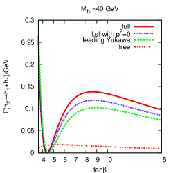
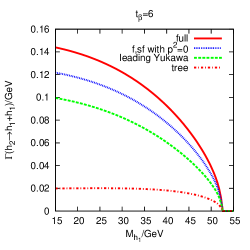
Figure 10: The decay width $\Gamma(h_{2}\to h_{1}h_{1})$ in the CPX scenario as a function of $\tan\beta$ at $M_{h_{1}}=40\,\,\mathrm{GeV}$ (left) and as a function of $M_{h_{1}}$ at $t_{\beta}=6$ (right). $M_{H^{\pm}}$ is adjusted to give the $M_{h_{1}}$ as required. All results include the propagator corrections. ‘tree’ indicates that the tree level triple Higgs vertex has been used. ‘leading Yukawa’ includes the leading genuine vertex corrections given in eqs. (6.1.1)–(97). ‘f,sf $p^{2}$=0’ includes contributions to the genuine vertex corrections from fermions and sfermions only and approximates the external momenta to zero. The curve labelled ‘full’ shows the result including the full genuine vertex corrections.

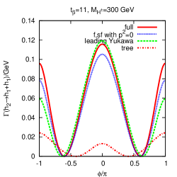
Figure 11: The dependence of the $h_{2}\to h_{1}h_{1}$ decay width on the phase $\phi=\phi_{A_{t}}=\phi_{A_{b}}=\phi_{A_{\tau}}=\phi_{M_{3}}$ ($\rm{CPX}$ scenario at $\tan\beta=11$, $M_{H^{\pm}}=300\,\,\mathrm{GeV}$). The full result is compared with different approximations, which are the same as those specified in Fig. 10.

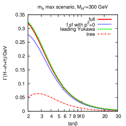
Figure 12: The decay width $\Gamma(H\to hh)$ in the $m_{h}^{\rm max}$ scenario as a function of $\tan\beta$ at $M_{H^{\pm}}=300\,\,\mathrm{GeV}$. The full result is compared with different approximations, which are the same as those specified in Fig. 10.

6.3.2 Effective coupling approximation for the lightest neutral Higgs boson

As we have seen, the effective triple Higgs vertices obtained using the leading corrections in the Yukawa approximation (as given in eqs. (6.1.1)–(97)) and the effective triple Higgs vertices obtained using the fermion/sfermion corrections at $p^{2}=0$ in the genuine vertex corrections and combining with the propagator corrections have both performed rather well as approximations to the $h_{2}\to h_{1}h_{1}$ or $H\to hh$ decay width. We have also seen that it is possible to get a large enhancement in these decay widths from the genuine vertex corrections. We shall now apply these approximations to the triple coupling of the lightest Higgs boson.

Fig. 13 shows this effective coupling squared, supplemented by propagator corrections and normalised to the tree level SM value (with equal Higgs mass). We can see that there is a suppression with respect to the tree level SM value if no genuine vertex corrections are included. This holds even in the limit of large $m_{A}$. This is because the SM tree-level coupling involves the square of the physical Higgs mass whereas the effective coupling in this limit involves the square of the tree-level mass of the lightest MSSM Higgs boson.

In Fig. 13, we also show the areas which are already excluded at the 95% CL by the LEP Higgs searches, which we have determined using the method described in Sect. 10.2 below. Including the genuine vertex corrections gives an overall enhancement of the effective couplings squared of approximately 1.2 to 1.6 in the parts of this parameter space which are not yet excluded. This could have interesting implications for the sensitivity of searches at the LHC and LC to effects of the triple-Higgs coupling in the MSSM.

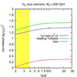
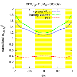
Figure 13: The triple coupling of the lightest Higgs boson squared, normalised to the SM tree-level value (with equal Higgs mass). Left: $m_{h}^{\rm max}$ scenario at $M_{H^{\pm}}=300\,\,\mathrm{GeV}$, varying $\tan{\beta}$. Right: $\rm{CPX}$ scenario, $t_{\beta}=11$, $M_{H^{\pm}}=300\,\,\mathrm{GeV}$, varying the phase $\phi=\phi_{A_{t}}=\phi_{A_{b}}=\phi_{A_{\tau}}=\phi_{M_{3}}$. All results include the propagator corrections. ‘tree’ indicates that the tree level triple Higgs vertex has been used. ‘leading Yukawa’ includes the leading genuine vertex corrections using the Yukawa approximation, as given in eqs. (6.1.1)–(97). ‘f,sf $p^{2}$=0’ includes contributions to the genuine vertex corrections from fermions and sfermions only and approximates the external momenta to zero. Yellow (shaded): excluded at 95% CL by the LEP Higgs searches (see Sect. 10.2 for details).

7 Higgs decay to SM fermions

7.1 Calculation of the $h_{a}\to b\bar{b}$ decay width

We use the general expression for two-body decay widths given in eq. (80) to obtain:

$$\Gamma(h_{a}\to b\bar{b}) = \frac{N_{c}}{8\pi M_{h_{a}}^{2}}\frac{M_{h_{a}}}{2}\sqrt{1-\frac{4m_{b}^{2}}{M_{h_{a}}^{2}}}\left|\mathcal{M}\right|^{2},$$ (114)

where $N_{c}$ is the number of colours. The mass dependence of the squared matrix element $\left|\mathcal{M}\right|^{2}$ will be affected by the CP properties of the Higgs boson. For example, at lowest order,

$$\Gamma_{\rm tree}(h_{a}\to b\bar{b}) = \frac{N_{c}}{8\pi}\frac{M_{h_{a}}}{2}\left(1-\frac{4m_{b}^{2}}{M_{h_{a}}^{2}}\right)^{x}\left|\lambda^{\rm tree}_{h_{a}b\bar{b}}\right|^{2},$$ (115)

where $\left|\lambda^{\rm tree}_{hb\bar{b}}\right|^{2}=\lambda_{b}^{(0),2}s^{2}_{\alpha}$, $\left|\lambda^{\rm tree}_{Hb\bar{b}}\right|^{2}=\lambda_{b}^{(0),2}c^{2}_{\alpha}$ and $\left|\lambda^{\rm tree}_{Ab\bar{b}}\right|^{2}=\lambda_{b}^{(0),2}s^{2}_{\beta}$ with $x=3/2$ for the CP even states $h,H$ and $x=1/2$ for the CP odd state $A$. $\lambda_{b}^{(0)}$ was defined in eq. (43).

7.1.1 Standard Model QED corrections

The real and virtual QED contributions to the Standard Model $H^{\rm SM}\rightarrow b\bar{b}$ decay width lead to the 1-loop correction

$$\Gamma_{\rm QED}(H^{\rm SM}\to b\bar{b}) = \Gamma_{\rm tree}(H^{\rm SM}\to b\bar{b})\left[1+\frac{\alpha}{\pi}Q_{b}^{2}\left(-3\log(\frac{M_{H^{\rm SM}}}{m_{b}})+\frac{9}{4}\right)\right],$$ (116)

for $M_{H}^{2,{\rm SM}}\gg m_{f}$, as derived in Ref. [123]. In this limit, this equation can be used for the QED corrections for both the scalar and pseudoscalar MSSM Higgs bosons[31]. We will therefore use the correction term

$$\delta_{\rm QED} := \frac{\alpha}{\pi}Q_{b}^{2}\left(-3\log(\frac{M_{h_{a}}}{m_{b}})+\frac{9}{4}\right)$$ (117)

in our MSSM calculation.

7.1.2 Standard Model QCD corrections

If the factor $Q_{b}^{2}\alpha$ in eq. (116) is replaced by the factor $C_{f}\alpha_{s}(M_{H}^{\rm SM})$, the expression for the 1-loop QCD correction to the $H^{\rm SM}\rightarrow b\bar{b}$ decay in the Standard Model is obtained, as shown in Ref. [123]. $C_{f}$ is the quadratic Casimir operator ($C_{f}=\frac{4}{3}$) and $\alpha_{s}(M_{H}^{2,{\rm SM}})$ is the running coupling. Including the tree level result gives

$$\Gamma_{\rm QCD}(H^{\rm SM}\to b\bar{b}) = \left[\frac{\Gamma^{\rm tree}(H^{\rm SM}\to b\bar{b})}{m_{b}^{2,OS}}\right]m_{b}^{2,OS}\left[1+\frac{\alpha_{s}(\mu_{\rm ren}^{2})}{\pi}C_{f}\left(-3\log(\frac{M_{H^{\rm SM}}}{m_{b}})+\frac{9}{4}\right)\right],$$

where we have factored out the Yukawa coupling from the term in the square bracket.

In the mass range we are interested in, $M_{H}^{\rm SM}\gg m_{b}$, this leading logarithmic approximation is not sufficient. However, the large logarithmic corrections can be absorbed into a running bottom quark mass. Substituting the relation between the on-shell b-quark mass and the running SM $\overline{\rm{MS}}$ b-quark mass into eq. (LABEL:hbbQCD1) gives

$$\Gamma_{\rm QCD}(H^{\rm SM}\to b\bar{b}) = \left[\frac{\Gamma^{\rm tree}(H^{\rm SM}\to b\bar{b})}{m_{b}^{2,OS}}\right]m_{b}^{2,\overline{\rm{MS}},SM}(\mu_{\rm ren})\left[1+\frac{\alpha_{s}(\mu_{\rm ren}^{2})}{4\pi}\left(-16\log(\frac{M_{H}}{\mu_{\rm ren}})+\frac{68}{3}\right)\right],$$

and we can choose $\mu_{\rm ren}=M_{H}^{\rm SM}$ in order to cancel the logarithmic term.

In practice, we parametrise our calculation in terms of $m_{b}^{\overline{\rm{MS}},SM}(M_{h_{a}})$. Therefore, in order to encompass the full 1-loop Standard Model-type QCD corrections in our calculation, we will need to add a correction

$$\delta_{\rm QCD}:=\frac{17}{3}\frac{\alpha_{s}(M_{h_{a}}^{2})}{\pi}$$ (120)

to the $h_{a}\to b\bar{b}$ decay width.

Our method differs from that of Ref. [30], which includes some higher order terms in $\alpha_{s}(\mu_{\rm ren}^{2})$ and $m_{b}^{\overline{\rm{MS}},SM}(\mu_{\rm ren})$ and an extra term proportional to $\alpha_{s}(m_{b}^{2})/\alpha_{s}(M_{h_{a}}^{2})$. Our method also differs from Ref. [94], which includes terms proportional to $\alpha_{s}^{2}$. However, some of these terms depend on the CP properties of the Higgs, and thus are not trivially extendable to the complex MSSM. Both Ref. [30] and Ref. [94] restrict their analyses to the MSSM with real parameters.

7.1.3 Full 1-loop 1PI $h_{i}\to b\bar{b}$ vertex corrections

In order to calculate the 1-particle irreducible vertex corrections at 1-loop, we have once again extended the FeynArts model file to include the relevant counterterms. We have evaluated the complete contributions in the MSSM, apart from the QED- and QCD-type corrections, for which we use the results given in eq. (117) and eq. (120), respectively. (Note that we include the photon contribution to the W boson mass counterterm). We include all complex phases. As discussed above, we use $m_{b}^{\overline{\rm{MS}},SM}(M_{h_{a}})$ in these corrections in order to absorb some of the higher order terms. As before, we use a unit CKM matrix and include no squark generation mixing.

7.1.4 Resummed $\Delta m_{b}$ corrections to $h_{i}\to b\bar{b}$

In order to resum the leading SUSY QCD (and higgsino) corrections for the case of large $\tan\beta$ in the limit of heavy SUSY particles, we use the effective vertices $v_{\rm h_{i}\bar{b}b}^{\Delta m_{b}}$ from the effective Langrangian in eq. (39).

$$v_{\rm h\bar{b}b}^{\Delta m_{b}} = \frac{1}{1+y}\left[1-\frac{1}{t_{\alpha}t_{\beta}}y+i\gamma_{5}x\left(1+\frac{1}{t_{\alpha}t_{\beta}}\right)\right]v_{\rm h\bar{b}b}^{\rm tree}$$

$$v_{\rm H\bar{b}b}^{\Delta m_{b}} = \frac{1}{1+y}\left[1+\frac{t_{\alpha}}{t_{\beta}}y+i\gamma_{5}x\left(1-\frac{t_{\alpha}}{t_{\beta}}\right)\right]v_{\rm H\bar{b}b}^{\rm tree}$$

$$v_{\rm A\bar{b}b}^{\Delta m_{b}} = \frac{1}{1+y}\left[1-\frac{1}{t_{\beta}^{2}}y+i\gamma_{5}x\left(1+\frac{1}{t_{\beta}^{2}}\right)\right]v_{\rm A\bar{b}b}^{\rm tree}.$$ (121)

When combining this contribution with the full genuine vertex corrections, we need to avoid double-counting of the 1-loop corrections involving gluinos or higgsinos. Therefore, we subtract the 1-loop part of these effective vertices, i.e. we use effective couplings of the form $\left(v_{\rm h_{i}\bar{b}b}^{\Delta m_{b}}-v_{\rm h_{i}\bar{b}b}^{\Delta m_{b},{\rm 1-loop}}\right)$ where

$$v_{\rm h\bar{b}b}^{\Delta m_{b},{\rm 1-loop}} = \left[{\rm Re}\Delta m_{b}\left(-1-\frac{1}{t_{\alpha}t_{\beta}}\right)+i\gamma_{5}{\rm Im}\Delta m_{b}\left(1+\frac{1}{t_{\alpha}t_{\beta}}\right)\right]v_{\rm h\bar{b}b}^{\rm tree},$$ (122)

$$v_{\rm H\bar{b}b}^{\Delta m_{b},{\rm 1-loop}} = \left[{\rm Re}\Delta m_{b}\left(-1+\frac{t_{\alpha}}{t_{\beta}}\right)+i\gamma_{5}{\rm Im}\Delta m_{b}\left(1-\frac{t_{\alpha}}{t_{\beta}}\right)\right]v_{\rm H\bar{b}b}^{\rm tree},$$ (123)

$$v_{\rm A\bar{b}b}^{\Delta m_{b},{\rm 1-loop}} = \left[{\rm Re}\Delta m_{b}\left(-1+\frac{1}{t_{\beta}^{2}}\right)+i\gamma_{5}{\rm Im}\Delta m_{b}\left(1+\frac{1}{t_{\beta}^{2}}\right)\right]v_{\rm A\bar{b}b}^{\rm tree}.$$ (124)

7.1.5 Combining these contributions with propagator corrections to obtain the full $h_{a}\to b\bar{b}$ decay width

The tree level, 1-loop 1PI $h_{i}\to b\bar{b}$ vertex function and the additional $\Delta m_{b}$ corrections are then combined with the propagator corrections from the $h_{i}h_{j}$ self-energies (via ${\mathbf{\hat{Z}}}$) and from the $h_{i}G$ and $h_{i}Z$ self-energies:

$$\Gamma_{h_{a}b\bar{b}} = {\mathbf{\hat{Z}}}_{ai}\left[\Gamma_{h_{i}b\bar{b}}^{\Delta m_{b},{\rm no\,1-loop}}+\Gamma_{h_{i}b\bar{b}}^{\rm 1PI,1-loop}\left(M^{2}_{h_{a}}\right)+\Gamma_{h_{i}b\bar{b}}^{\rm G,Z\,se}\left(m^{2}_{h_{i}}\right)\right].$$ (125)

The arguments to $\Gamma_{h_{i}b\bar{b}}^{\rm 1PI,1-loop}$ and $\Gamma_{h_{i}b\bar{b}}^{\rm G,Z\,se}$ denote the external momenta used. $\Gamma_{h_{i}b\bar{b}}^{\Delta m_{b},{\rm no\,1-loop}}$ denotes the use of $\left(v_{\rm h_{i}\bar{b}b}^{\Delta m_{b}}-v_{\rm h_{i}\bar{b}b}^{\Delta m_{b},{\rm 1-loop}}\right)$. $\Gamma_{h_{a}b\bar{b}}$ is combined with the external fermion wavefunctions, then we take the squared modulus and sum over external spins to get $|\mathcal{M}_{h_{a}b\bar{b}}|^{2}$.

The full $h_{a}\to b\bar{b}$ decay width is thus found using

$$\Gamma^{\rm full}(h_{i}\to b\bar{b}) = \left[1+\delta_{\rm QCD}+\delta_{\rm QED}\right]\frac{N_{c}}{8\pi M_{h_{a}}^{2}}\frac{M_{h_{a}}}{2}\sqrt{1-\frac{4m_{b}^{2}}{M_{h_{a}}^{2}}}\left|\mathcal{M}_{h_{a}b\bar{b}}\right|^{2},$$ (126)

which is an extension of the method used to combine QED, QCD and Z-factor corrections in Ref. [30].

7.1.6 Numerical Results

Fig. 14 illustrates the decay widths $\Gamma(h_{1}\to b\bar{b})$ (left), $\Gamma(h_{2}\to b\bar{b})$ (centre) and $\Gamma(h_{3}\to b\bar{b})$ (right) as a function of the charged Higgs mass for the CPX scenario with $\tan\beta=20$. All results include the propagator corrections, incorporated via the matrix ${\mathbf{Z}}$, and the Goldstone and gauge boson mixing contribution. We note that the $h_{1}$ and $h_{2}$ decay widths have steep gradients at $M_{H^{\pm}}\sim 157\,\,\mathrm{GeV}$ due to a ‘cross-over’ effect in the masses (i.e. $M_{h_{1}}$ and $M_{h_{2}}$ approach each other). At $M_{H^{\pm}}\sim 150\,\,\mathrm{GeV}$, $h_{1}$ is mostly $A$, $h_{2}$ is mostly $h$ and $h_{3}$ is mostly $H$, whereas at $M_{H^{\pm}}\sim 200\,\,\mathrm{GeV}$, $h_{1}$ is mostly $h$, $h_{2}$ is mostly $A$ and $h_{3}$ is mostly $H$.

The impact of including the resummed $\Delta m_{b}$ contributions is very significant, as we can see from comparison of the result using the propagator, SM QCD and QED corrections (‘QED, QCD’) and the result when the resummed $\Delta m_{b}$ contributions are included in addition (‘QED, QCD, $\Delta m_{b}$’). Fig. 14 also includes the full decay widths (‘full’), which combine the propagator, QED, SM QCD, SUSY QCD corrections with the full electroweak genuine vertex corrections, as described by eq. (126), and the effect of including the full corrections turns out to be relatively small but not negligible. At $M_{H^{\pm}}=600\,\,\mathrm{GeV}$, these extra electroweak corrections are 5.6%, 5.7% and 5.0% for the decay of $h_{1},h_{2},h_{3}$, respectively.

It is possible to approximate the ‘QED, QCD, $\Delta m_{b}$’ result using an effective $b$-quark mass of $m_{b}^{\overline{\rm{MS}},SM}(m_{t})/|1+\Delta m_{b}|$ (with no additional $\Delta m_{b}$ contributions), which we call ‘QED, QCD, effective $m_{b}$’. The resulting decay widths are also shown in Fig. 14. In general, this approximation performs well. However, note that in the decoupling limit, where the $h_{1}$ is SM-like, the effect of the SUSY QCD corrections should cancel out in the $h_{1}$ decay width. In the approximate ‘QED, QCD, effective $m_{b}$’ result, this does not occur, giving a offset which is significant in relative terms, although small in absolute terms. In the region $M_{H^{\pm}}=200\,\,\mathrm{GeV}$ to $M_{H^{\pm}}=600\,\,\mathrm{GeV}$ shown here, this offset between the ‘QED, QCD, effective $m_{b}$’ result and the approximate result is more than 44% of the ‘QED, QCD, $\Delta m_{b}$’ result, while the absolute difference is less than $0.002\,\,\mathrm{GeV}$.

The $h_{a}\to b\bar{b}$ decay width in the $\rm{CPX}$ scenario is highly dependent on $\phi_{M_{3}}$. Fig. 15 shows the decay widths of the two lightest Higgs bosons into b-quarks at $\phi_{M_{3}}=0$, $\phi_{M_{3}}=\pi/2$ and $\phi_{M_{3}}=3\pi/4$. Whereas the inclusion of the resummed $\Delta m_{b}$-type corrections suppresses the decay width at $\phi_{M_{3}}=0$, at $\phi_{M_{3}}=\pi/2$ and $\phi_{M_{3}}=3\pi/4$ these corrections have caused an enhancement. The value of $\Delta m_{b}$ in these plots is $1.05-0.12i$, $-1.16i$,$-0.75-0.86i$ for $\phi_{M_{3}}=0$, $\phi_{M_{3}}=\pi/2$ and $\phi_{M_{3}}=3\pi/4$, respectively.

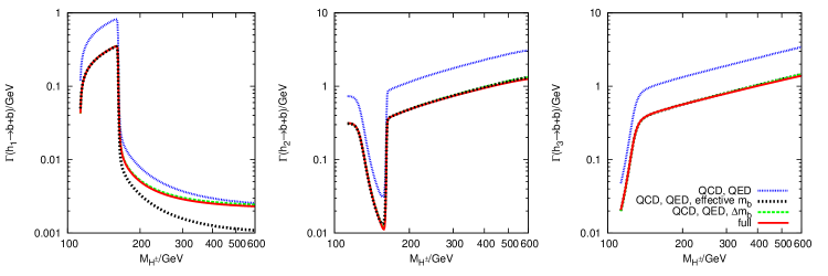
Figure 14: The decay widths of the neutral Higgs bosons to two b-quarks in the $\rm{CPX}$ scenario with $\tan\beta=20$. See text for explanation of the various approximations used.

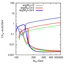
Figure 15: The decay widths of the two lightest neutral Higgs bosons to two b-quarks in the $\rm{CPX}$ scenario with $\tan\beta=20$ at various values of $\phi_{M_{3}}$. Solid: $h_{a}=h_{1}$, dashed: $h_{a}=h_{2}$.

7.2 Calculation of the $h_{a}\to\tau^{+}\tau^{-}$ decay width

The calculation of the $h_{a}\to\tau^{+}\tau^{-}$ decay width is similar to that of the $h_{a}\to b\bar{b}$ decay width, with the simplification that no QCD corrections are required. We have calculated the full 1-loop genuine vertex corrections and supplemented these with propagator corrections (including 1-loop mixing with Goldstone and Z bosons) and QED corrections. As before, we have included all complex phases.

8 Higgs cascade decay branching ratios

Accurate predictions for Higgs branching ratios are vital for Higgs phenomenology. In particular, they are required as part of calculations of cross sections of collider processes involving the production and decay of an on-shell Higgs boson, which are often performed using the narrow width approximation. In Sect. 10.2, we will use Higgs branching ratios for the CPX scenario in conjunction with the LEP topological cross section limits. In order to understand the resulting exclusions, it will be necessary to refer to the behaviour of the contributing branching ratios.

We combine the $h_{a}\to h_{b}h_{c}$ decay widths calculated in Sect. 6 with the $h_{a}\to b\bar{b}$ and $h_{a}\to\tau^{-}\tau^{+}$ decay widths calculated in Sect. 7. As we have discussed, these decay widths include the full 1-loop genuine vertex corrections and are combined with propagator corrections obtained using neutral Higgs self-energies from the program FeynHiggs [6, 7, 8, 9, 10], which include the leading 2-loop contributions. The 1-loop propagator mixing with Goldstone and Z bosons is also consistently incorporated. These results take into account the full phase dependence of the supersymmetric parameters. For the $h_{a}\to b\bar{b}$ decay width, the $\Delta m_{b}$ corrections are resummed in a way that preserves the phase dependence. We take all other decay widths from the program FeynHiggs [6, 7, 8, 9, 10] (these decay modes are subdominant in most of the regions of MSSM parameter space).

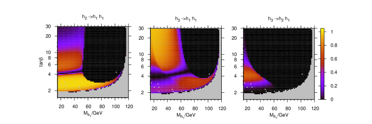
Figure 16: The branching ratios of neutral Higgs bosons into other neutral Higgs bosons in the $\rm{CPX}$ scenario.

Fig. 16 (left plot) illustrates the pronounced dependence of the $h_{2}\to h_{1}h_{1}$ branching ratio on $\tan\beta$ and $M_{h_{1}}$. We see that this decay mode is significant and often dominant in almost all of the regions where it is kinematically allowed. We can see that the characteristics of the $h_{2}\to h_{1}h_{1}$ branching ratio are largely determined by the behaviour of the $h_{2}\to h_{1}h_{1}$ decay widths (in Fig. 10 we showed this decay width for two slices of $\rm{CPX}$ parameter space). Note, in particular, the narrow ‘knife-edge’ region of very low $h_{2}\to h_{1}h_{1}$ branching ratio, which occurs at $\tan\beta\sim 4.5$, where the $h_{2}\to h_{1}h_{1}$ decay width tends to zero. The behaviour of the $h_{2}\to b\bar{b}$ branching ratio is also heavily dependent on the $h_{2}\to h_{1}h_{1}$ decay width where the $h_{2}\to h_{1}h_{1}$ decay is allowed kinematically, since in this region, the $h_{2}\to h_{1}h_{1}$ decay usually makes up the majority of the total decay width. Over the majority of $\rm{CPX}$ parameter space, BR($h_{2}\to h_{1}h_{1}$)+BR($h_{2}\to b\bar{b})$+BR($h_{2}\to\tau^{+}\tau^{-}$)$\sim 1$, and BR($h_{2}\to\tau^{+}\tau^{-}$) is comparatively small.

The Higgs cascade decays for the heaviest neutral Higgs $h_{3}$ also dominate in the majority of the region where they are kinematically allowed. The $h_{3}\to h_{1}h_{1}$ branching ratio (middle plot of Fig. 16) also has a narrow region at $\tan\beta\sim 4-5$ in which, while the $h_{3}\to h_{1}h_{1}$ decay is kinematically allowed, the decay width is nevertheless suppressed, characteristically similar to the suppressed region we observed in the $h_{2}\to h_{1}h_{1}$ branching ratio. In particular, topologies involving $h_{3}$ can be relevant to the LEP exclusions in the region $10\;\raisebox{-3.00003pt}{$\stackrel{{\scriptstyle\displaystyle<}}{{\sim}}$}\;\tan\beta\;\raisebox{-3.00003pt}{$\stackrel{{\scriptstyle\displaystyle<}}{{\sim}}$}\;30$, $M_{h_{1}}\;\raisebox{-3.00003pt}{$\stackrel{{\scriptstyle\displaystyle<}}{{\sim}}$}\;60\,\,\mathrm{GeV}$ for variations of the CPX scenario. In this region of parameter space, the $h_{3}\to h_{1}h_{1}$ decay width is a crucial contribution also to the $h_{3}\to b\bar{b}$ branching ratio. The $h_{3}\to h_{2}h_{1}$ decay width (the $h_{3}\to h_{2}h_{1}$ branching ratio is shown in the right plot of Fig. 16), on the other hand, is of less phenomenological interest in this scenario, since this decay width dominates the total $h_{3}$ width in a region which, as we will see, can be excluded at the 95% CL using limits on the cross sections of topologies involving $h_{1}$ and $h_{2}$.

9 Normalised $e^{+}e^{-}$ Higgsstrahlung and pair production cross sections

In order to examine the effect of our predictions for the Higgs branching ratios on the size of the regions of $\rm{CPX}$ parameter space which can be excluded by the LEP Higgs searches, we need to consider the Higgsstrahlung and Higgs pair production cross sections, normalised to a reference cross section $\sigma_{\rm ref}$. In the MSSM with real parameters, the corrections to the LEP Higgsstrahlung and LEP pair production processes have been studied in detail [34, 35, 36, 37, 38, 39]. In the MSSM with CP violation, there has also been considerable interest in accurate predictions of these cross sections, although the full 1-loop corrections are not yet available [40, 41, 42, 43, 44].

For the Higgsstrahlung topologies $e^{+}e^{-}\rightarrow h_{a}Z$, the reference cross section $\sigma_{\rm ref}$ is the tree level SM cross section for the process $e^{+}e^{-}\rightarrow Z\rightarrow HZ$, for a SM-like Higgs of mass $M_{H}=M_{h_{a}}$. For the pair production topologies $e^{+}e^{-}\rightarrow h_{a}h_{b}$, the reference cross section $\sigma_{\rm ref}$ is the tree level MSSM cross section for the process $e^{+}e^{-}\rightarrow Z\rightarrow h^{0}A^{0}$, where the MSSM coupling factor $\cos^{2}{(\beta-\alpha)}$ has been divided out and the masses of $h^{0}$ and $A^{0}$ taken as $M_{h_{a}}$ and $M_{h_{b}}$ respectively. This reference cross section can also be expressed in terms of the Standard Model Higgsstrahlung production cross section,

$$\sigma_{\rm ref}=\bar{\lambda}\sigma^{\rm SM}(e^{+}e^{-}\rightarrow HZ),$$ (127)

where $\bar{\lambda}$ is a kinematic factor which takes into account the different kinematic dependences of the SM Higgsstrahlung and the pair production process, i.e.

$$\bar{\lambda} = \lambda^{3/2}_{h_{a}h_{b}}/\left(12M_{Z}^{2}/s+\lambda_{ZH}\right)/\lambda^{1/2}_{ZH},$$ (128)

$$\lambda_{xy} = \left[1-\left(M_{x}+M_{y}\right)^{2}/s\right]\left[1-\left(M_{x}-M_{y}\right)^{2}/s\right],$$ (129)

and $H$ is a SM-like Higgs with mass $M_{H}$.

For the majority of our scans, we will calculate these normalised cross sections using an effective coupling for the $h_{a}$-$Z$-$Z$ or $h_{a}$-$h_{b}$-$Z$ vertex, which incorporates external Higgs propagator corrections. However, we will also examine the effect of including the complete $t,\tilde{t},b,\tilde{b}$ 1-loop corrections (involving also genuine vertex corrections) in these cross sections.

9.1 Normalised effective Higgs couplings to gauge bosons

The matrix ${\mathbf{Z}}$ can be used to create a normalised effective coupling between neutral Higgs bosons and Z bosons which takes the corrections to the external Higgs propagators into account, though the relations

$$g^{\rm eff}_{h_{a}ZZ} = {\mathbf{Z}}_{ai}g^{\rm tree}_{h_{i}ZZ},$$ (130)

$$g^{\rm eff}_{h_{a}h_{b}Z} = {\mathbf{Z}}_{bj}{\mathbf{Z}}_{ai}g^{\rm tree}_{h_{i}h_{j}Z},$$ (131)

where $g^{\rm tree}_{h_{i}ZZ}$ are normalised to the SM coupling, such that $(g^{{\rm tree}}_{hZZ})^{2}=\sin^{2}{(\beta-\alpha)}$, $(g^{{\rm tree}}_{HZZ})^{2}=\cos^{2}{(\beta-\alpha)}$ and $(g^{{\rm tree}}_{AZZ})^{2}=0$. In addition, we normalise the $g^{\rm tree}_{h_{i}h_{j}Z}$ such that $(g^{{\rm tree}}_{hAZ})^{2}=\cos^{2}{(\beta-\alpha)}$ and $(g^{{\rm tree}}_{HAZ})^{2}=\sin^{2}{(\beta-\alpha)}$. All other $g^{\rm tree}_{h_{i}h_{j}Z}$ are zero.

Fig. 17 illustrates the normalised squared effective Higgs couplings to gauge bosons $|g^{{\rm eff}}_{h_{a}ZZ}|^{2}$ in the CPX scenario. We can see that the $h_{1}$-$Z$-$Z$ coupling dominates around the edge of the available parameter space, the $h_{3}$-$Z$-$Z$ coupling dominates in a region $M_{h_{1}}<60\,\,\mathrm{GeV}$ and $7\;\raisebox{-3.00003pt}{$\stackrel{{\scriptstyle\displaystyle<}}{{\sim}}$}\;\tan\beta$, and the $h_{2}$-$Z$-$Z$ coupling dominates the region in between, such that $|g^{{\rm eff}}_{h_{1}ZZ}|^{2}+|g^{{\rm eff}}_{h_{2}ZZ}|^{2}+|g^{{\rm eff}}_{h_{3}ZZ}|^{2}\sim 1$. Fig. 18 illustrates the behaviour of $|g^{{\rm eff}}_{h_{a}h_{b}Z}|^{2}$, which can be described as $|g_{h^{{\rm eff}}_{a}ZZ}|^{2}\sim|g^{{\rm eff}}_{h_{b}h_{c}Z}|^{2}$, where $h_{a},h_{b},h_{c}$ are all different. (If a unitary approximation to the ${\mathbf{Z}}$ matrix is used, as in the LEP Higgs Working Group analysis of the $\rm{CPX}$ scenario[2], these relations become equalities.)

The normalised Higgsstrahlung and pair production cross sections can then be approximated by these effective couplings, i.e

$$\sigma(e^{+}e^{-}\rightarrow h_{a}Z)/\sigma_{\rm ref} = |g^{{\rm eff}}_{h_{a}ZZ}|^{2},$$ (132)

$$\sigma(e^{+}e^{-}\rightarrow h_{a}h_{b})/\sigma_{\rm ref} = |g^{{\rm eff}}_{h_{a}h_{b}Z}|^{2}.$$ (133)

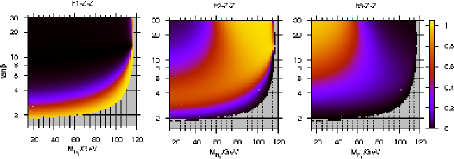
Figure 17: The effective couplings of the neutral Higgs bosons to two $Z$ bosons, $|g^{{\rm eff}}_{h_{1}ZZ}|^{2}$,$|g^{{\rm eff}}_{h_{2}ZZ}|^{2}$ and $|g^{{\rm eff}}_{h_{3}ZZ}|^{2}$, which include the Higgs propagator corrections calculated using the matrix ${\mathbf{\hat{Z}}}$.

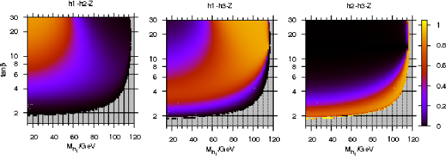
Figure 18: The effective couplings of two neutral Higgs bosons to a $Z$ boson, $|g^{{\rm eff}}_{h_{1}h_{2}Z}|^{2}$,$|g^{{\rm eff}}_{h_{1}h_{3}Z}|^{2}$ and $|g^{{\rm eff}}_{h_{2}h_{3}Z}|^{2}$, which include the Higgs propagator corrections calculated using the matrix ${\mathbf{\hat{Z}}}$.

9.2 Loop corrections to the Higgsstrahlung and pair production cross sections

Figure 19: Additional corrections to the Higgsstrahlung and pair production processes. The grey circles indicate loops involving $t,\tilde{t},b,\tilde{b}$ and $X_{I},X_{J}=(h,H,A,G,Z)$. Note that not all of the combinations are physical, since the tree level vertices must be CP-conserving. In addition, we neglect the electron mass, therefore no contributions where a Higgs boson couples to the electrons are included.

We now consider 1-loop corrections to the LEP Higgsstrahlung and pair production processes involving the particles $t,\tilde{t},b,\tilde{b}$. The structure of these diagrams is shown in Fig. 19, where loops involving $t,\tilde{t},b,\tilde{b}$ are indicated by grey circles. In general, lines labelled with $X$ can be $h,H,A,G,Z$, where the resulting diagram conserves CP at the tree level vertices involving the gauge and Higgs bosons. We neglect the electron mass and therefore will not include any diagrams in which a Higgs boson couples directly to the electrons. We then include the Higgs propagator factors for the Higgs on external legs through the ${\mathbf{Z}}$ matrix, as previously.

The result of including these corrections on the normalised Higgsstrahlung cross section in the $\rm{CPX}$ scenario at $M_{h_{1}}=40\,\,\mathrm{GeV}$ is given in Fig. 20 (left). The dashed lines show the result for the tree level $h_{i}$-$Z$-$Z$ vertex combined with Higgs propagator factors, using eq. (130). The solid lines show the result when the full $t,\tilde{t},b,\tilde{b}$ 1-loop corrections are also included. Similarly, the dashed lines in Fig. 20 (right) show the normalised pair production cross sections using eq. (131), and the solid lines show the result if the $t,\tilde{t},b,\tilde{b}$ 1-loop corrections are also used. The effect of including the $t,\tilde{t},b,\tilde{b}$ corrections turns out to be negligible for the Higgsstrahlung process. However, for the pair production process, a more sizable effect is visible, leading to an increase of the normalised cross section. This is due to the additional Yukawa coupling in the genuine vertex corrections of the Higgs pair production process as compared to the Higgsstrahlung process, so that a larger enhancement factor is possible in this case. As will be discussed in the follwing section, the impact of this kind of corrections on the coverage of the LEP Higgs searches in the CPX scenario is nevertheless rather small.

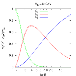
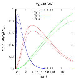
Figure 20: The normalised Higgsstrahlung cross sections (left) and normalised pair production cross sections (right) in the $\rm{CPX}$ scenario at $M_{h_{1}}=40\,\,\mathrm{GeV}$. Dashed lines: using eq. (130) or eq. (131). Solid lines: as for the dashed lines except that the $t,\tilde{t},b,\tilde{b}$ 1-loop corrections are also included (neglecting the electron mass).

10 Confronting the Higgs sector predictions with limits from the LEP Higgs searches

10.1 LHWG limits on the parameter space of the $\rm{CPX}$ scenario

After the LEP programme finished in 2000, the final results from the four LEP collaborations (ALEPH [1, 124, 125], DELPHI [126, 127], L3 [128] and OPAL [129, 130]) were combined and examined for consistency with a background hypothesis and a signal plus background hypothesis in a coordinated effort between the LEP Higgs Working Group for Higgs Searches and the LEP collaborations (LHWG). The results showed no significant excess of events which would indicate the production of a Higgs boson. In the Standard Model, a lower bound on the Higgs mass of $114.4\,\,\mathrm{GeV}$ at the 95% confidence level was established [1], while restrictions were placed on the available parameter space of a variety of MSSM benchmark scenarios [2], including the $\rm{CPX}$ scenario[5].

For the purposes of the LHWG analysis, two different programs were used to calculate Higgs masses and branching ratios in the complex MSSM: FeynHiggs version 2.0 [10] and CPH [5], which was a predecessor of the program CPsuperH [11, 12]. These two codes had significant differences in the incorporated higher order corrections, and it was necessary to perform a conversion between the two sets of input parameters, due to the different renormalisation schemes used in the two codes. As explained below, the parameter conversion used was an approximation based on a calculation performed in the MSSM with real parameters.

Separate analyses were performed using FeynHiggs and CPH. In order to combine these results, a conservative method was adopted, in which a point in parameter space was regarded as excluded only if it was excluded by both the analysis using results from FeynHiggs and the analysis using results from CPH. The LHWG analysis resulted in three unexcluded regions of $\rm{CPX}$ parameter space at 95 % CL:

• (A) $60\,\,\mathrm{GeV}\;\raisebox{-3.00003pt}{$\stackrel{{\scriptstyle\displaystyle<}}{{\sim}}$}\;M_{h_{1}}$ and $3\;\raisebox{-3.00003pt}{$\stackrel{{\scriptstyle\displaystyle<}}{{\sim}}$}\;\tan\beta$

• (B) $30\,\,\mathrm{GeV}\;\raisebox{-3.00003pt}{$\stackrel{{\scriptstyle\displaystyle<}}{{\sim}}$}\;M_{h_{1}}\;\raisebox{-3.00003pt}{$\stackrel{{\scriptstyle\displaystyle<}}{{\sim}}$}\;50\,\,\mathrm{GeV}$ and $3\;\raisebox{-3.00003pt}{$\stackrel{{\scriptstyle\displaystyle<}}{{\sim}}$}\;\tan\beta\;\raisebox{-3.00003pt}{$\stackrel{{\scriptstyle\displaystyle<}}{{\sim}}$}\;10$

• (C) $0\,\,\mathrm{GeV}\;\raisebox{-3.00003pt}{$\stackrel{{\scriptstyle\displaystyle<}}{{\sim}}$}\;M_{h_{1}}\;\raisebox{-3.00003pt}{$\stackrel{{\scriptstyle\displaystyle<}}{{\sim}}$}\;10\,\,\mathrm{GeV}$ and $3\;\raisebox{-3.00003pt}{$\stackrel{{\scriptstyle\displaystyle<}}{{\sim}}$}\;\tan\beta\;\raisebox{-3.00003pt}{$\stackrel{{\scriptstyle\displaystyle<}}{{\sim}}$}\;20$

The results from the separate FeynHiggs and CPH analyses showed substantial differences. In particular, the FeynHiggs analysis had a larger unexcluded region of type B, and the CPH analysis had a larger unexcluded region of type A, while both results showed similar unexcluded regions of type C. We shall concentrate on unexcluded regions of type A and B in this paper, since constraints other than those from Higgs searches play a role in the unexcluded region C (see, e.g., Ref. [131] for a discussion of region C).

There was an additional complication, since FeynHiggs as yet does not have a reliable calculation for the loop corrections to the triple Higgs couplings in the CP-violating MSSM. For the purposes of the ‘FeynHiggs’ analysis, the triple Higgs coupling was therefore obtained from CPH, and then combined with Higgs masses and other Higgs sector quantities as calculated by FeynHiggs[2]. As we will see, higher order corrections to the triple Higgs coupling have a great influence on the size, shape and position of the unexcluded region B.

10.2 The effect of the new Higgs sector corrections on the limits on the parameter space of the $\rm{CPX}$ scenario

The LEP Higgs Working Group for Higgs Searches and the LEP collaborations also published their combined results in the form of topological cross section limits at 95% CL, which can be applied to a wide range of theoretical models. In each of these topologies, the Higgs is produced either through Higgsstrahlung or pair production and decays either to b-quarks, tau-leptons or via the Higgs cascade decay. To a very good approximation, the kinematic distributions of these processes are independent of the CP properties of the Higgs bosons involved, as discussed in Ref. [2]. Therefore, the same topological bounds can be used for CP-even, CP-odd or mixed CP Higgs bosons.

In this section, we will use the topological cross section limits from LEP in conjunction with updated predictions for the Higgs masses, couplings and branching ratios. In particular, we shall be using our full 1-loop diagrammatic calculation for the $h_{i}\to h_{j}h_{k}$ decay processes with full phase dependence as described in Sect. 6, combined with renormalised neutral Higgs self-energies obtained from the current version of FeynHiggs (which includes corrections at $\mathcal{O}(\alpha_{t}\alpha_{s})$ with full phase dependence).

In order to utilise the cross section limits, we use the program HiggsBounds [57, 58]. As input, it requires the Higgs masses, the normalised production cross sections and the branching ratios BR($h_{a}\to h_{b}h_{b}$), BR($h_{a}\to b\bar{b}$) and BR($h_{a}\to\tau^{+}\tau^{-}$) for each parameter point. We obtain the Higgs masses as described in Sect. 4 and we calculate the Higgs branching ratios as described in Sect. 6. We will begin by using LEP Higgsstrahlung production cross sections which include both the full propagator corrections and additional $t,\tilde{t},b,\tilde{b}$ corrections, as discussed in Sect. 9.2. Unless otherwise stated, we will investigate the CPX scenario, as defined in Sect. 3 and, unless explicitly stated, we do not consider the possible impact of theoretical uncertainties from unknown higher order corrections on the exclusion bounds in the parameter space.

HiggsBounds uses the provided Higgs sector predictions to determine which process has the highest statistical sensitivity for setting an exclusion limit for each parameter point, using the median expected limits based on Monte Carlo simulations with no signal. It then compares the theoretical cross section for this particular process with the experimentally observed limit for this process. In this way, only one topological limit is used for each parameter point, thus ensuring that any resulting exclusion is valid at the 95% CL.

However, it should be noted that, in general, the dedicated analyses carried out in Ref. [2] for specific MSSM benchmark scenarios have a higher exclusion power than analyses using HiggsBounds, since, in a dedicated analysis, the information from different search channels can be combined. This can, in particular, lead to an improved result in regions of parameter space where several channels have similar statistical sensitivities.

Fig. 21 (left) indicates which channel has the highest sensitivity and therefore which channel will be used for each point in CPX parameter space, to determine whether or not it is excluded at the 95 % CL. The channel $h_{1}Z\to b\bar{b}Z\,({\color[rgb]{1,0,0}\blacksquare})$ has the highest statistical sensitivity at the edge of the $\rm{CPX}$ parameter space where $\tan\beta$ is low or $M_{h_{1}}$ is high, due to the fact that the coupling of the lightest Higgs boson to two Z bosons is unsuppressed in this region, as we saw in Fig. 17. Similarly, in a band adjacent to this, where the coupling of the second heaviest Higgs boson to two Z bosons is unsuppressed, the Higgstrahlung processes $h_{2}Z\to b\bar{b}Z\,({\color[rgb]{0,0,1}\blacksquare})$ and $h_{2}Z\to h_{1}h_{1}Z\to b\bar{b}b\bar{b}Z\,(\square)$ have the highest statistical sensitivity. Finally, in the upper left region of the plot, where $|g^{{\rm eff}}_{h_{1}h_{2}Z}|^{2}$ is high, the pair production processes $h_{2}h_{1}\to b\bar{b}b\bar{b}\,({\color[rgb]{0,1,1}\blacksquare})$ and $h_{2}h_{1}\to h_{1}h_{1}h_{1}\to b\bar{b}b\bar{b}b\bar{b}\,({\color[rgb]{1,1,0}\blacksquare})$ have the highest statistical sensitivity. The part of the parameter space in which the processes directly involving the $h_{2}\to h_{1}h_{1}$ decay ($h_{2}Z\to h_{1}h_{1}Z\to b\bar{b}b\bar{b}Z\,(\square)$ and $h_{2}h_{1}\to h_{1}h_{1}h_{1}\to b\bar{b}b\bar{b}b\bar{b}\,({\color[rgb]{1,1,0}\blacksquare})$) dominate occurs in a region with an increased $h_{2}\to h_{1}h_{1}$ branching ratio at $\tan\beta\sim 5-10$, as we saw in Fig. 16 (left), and which is influenced by the peak in the $h_{2}\to h_{1}h_{1}$ decay width as shown in Fig. 10 (left) at $\tan\beta\sim 8$. Fig. 21 (right) differs from Fig. 21 (left) in that only the propagator corrections have been used when calculating the predictions for the LEP Higgs production cross sections (i.e. we use the normalised squared effective couplings $|g^{{\rm eff}}_{h_{a}ZZ}|^{2}$ and $|g^{{\rm eff}}_{h_{a}h_{b}Z}|^{2}$ described in Sect. 9.2). We see that the graphs are very similar, with the main difference being the reduced size of the $h_{1}Z\to b\bar{b}Z\,({\color[rgb]{1,0,0}\blacksquare})$ region at $\tan\beta\sim 5$, $M_{h_{1}}\sim 25\,\,\mathrm{GeV}$.

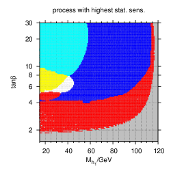
Figure 21: The coverage of the LEP Higgs searches in the $M_{h_{1}}$–$\tan\beta$ plane of the CPX scenario, showing the channels that are predicted to have the highest statistical sensitivity for setting an exclusion limit. The colour codings are: red = $h_{1}Z\to b\bar{b}Z\,({\color[rgb]{1,0,0}\blacksquare})$, blue = $h_{2}Z\to b\bar{b}Z\,({\color[rgb]{0,0,1}\blacksquare})$, white = $h_{2}Z\to h_{1}h_{1}Z\to b\bar{b}b\bar{b}Z\,(\square)$, cyan = $h_{2}h_{1}\to b\bar{b}b\bar{b}\,({\color[rgb]{0,1,1}\blacksquare})$, yellow = $h_{2}h_{1}\to h_{1}h_{1}h_{1}\to b\bar{b}b\bar{b}b\bar{b}\,({\color[rgb]{1,1,0}\blacksquare})$, green = $h_{3}h_{1}\to b\bar{b}b\bar{b}\,({\color[rgb]{0,1,0}\blacksquare})$, purple = other channels (${\color[rgb]{0,0,0}\blacksquare}$). Left: full result (i.e. including the extra corrections to the Higgstrahlung and pair production cross sections described in Sect. 9.2). Right: using effective coupling approximation for production cross sections.

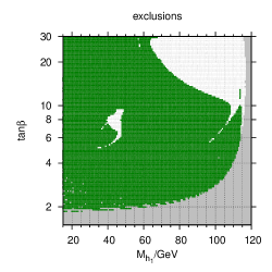
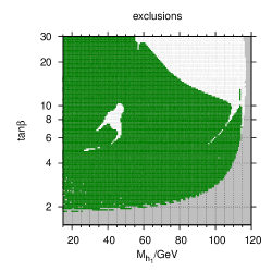
Figure 22: The coverage of the LEP Higgs searches in the $M_{h_{1}}$–$\tan\beta$ plane of the CPX scenario, showing the parameter regions excluded at the 95% C.L. by the topological cross section limits obtained at LEP. The colour codings are: green (darker grey) = LEP excluded, white = LEP allowed. Left: full result (i.e. including the extra corrections to the Higgstrahlung and pair production cross sections described in Sect. 9.2). Right: using effective coupling approximation for production cross sections.

In Fig. 22 (left), we have compared our theoretical cross section predictions for each parameter point in the CPX scenario with the observed topological cross section limits obtained at LEP for the channel with the highest statistical sensitivity at that point, in order to obtain exclusions at 95% CL. The Higgsstrahlung topologies where the Higgs decays to b-quarks are unable to exclude Higgs masses above $M_{h_{1}}\;\raisebox{-3.00003pt}{$\stackrel{{\scriptstyle\displaystyle>}}{{\sim}}$}\;114.4\,\,\mathrm{GeV}$, as we would expect, since this is the limit on the mass of a SM-like Higgs boson [1]. The upper edge of the excluded area in the $h_{2}Z\to b\bar{b}Z\,({\color[rgb]{0,0,1}\blacksquare})$ region has a similar shape to the $M_{h_{2}}\;\raisebox{-3.00003pt}{$\stackrel{{\scriptstyle\displaystyle>}}{{\sim}}$}\;114.4\,\,\mathrm{GeV}$ contour and, at $\tan\beta=20$, occurs at a position $\Delta M_{h_{2}}\sim 4\,\,\mathrm{GeV}$ relative to it. As before, we call the unexcluded area in the top right region of the plot, ‘unexcluded region A’. It has a narrow ‘tail’, which extends to lower $\tan\beta$, one side of which is bounded by the limit for a SM-like $M_{h_{2}}$ and one side of which is bounded by the edge of the region where the channel $h_{1}Z\to b\bar{b}Z\,({\color[rgb]{1,0,0}\blacksquare})$ has the highest statistical significance, as shown in Fig. 21 (left). Fig. 22 (right) differs from Fig. 22 (left) in that only the propagator corrections have been used when calculating the predictions for the LEP Higgs production cross sections. Once again, we see that the extra $t,\tilde{t},b,\tilde{b}$ corrections only have a very small numerical effect. Therefore, we will neglect these corrections in the results that we show below.

The plots in Fig. 22 also show an unexcluded region of type B at $M_{h_{1}}\sim 45\,\,\mathrm{GeV}$ and $\tan\beta\sim 8$. From comparison with Fig. 16 (left), we can see that the entire unexcluded region B in Fig. 22 lies in an area where the $h_{2}\to h_{1}h_{1}$ branching ratio is sizable. We examine this unexcluded region B in more detail in Fig. 23 (top row), where we show an enlarged version of the relevant part of parameter space from Fig. 21 (right) and Fig. 22 (right). As we can see, the two thin extensions of the unexcluded region both lie along boundaries between areas where different processes have the highest statistical significance. As we have discussed, we would expect our method of combining channels (which only makes use of one observed limit for each parameter point) to be less effective at such boundaries. Thus, a dedicated analysis including the combination of different channels might well be able to exclude such areas.

The results presented here update our previous result[22] in two main ways. Most importantly, we now use a newer version of FeynHiggs [6, 7, 8, 9, 10] to obtain the neutral Higgs self-energies, with an improved treatment of the $\tan{\beta}$ enhanced contributions. In addition, Ref. [22] uses $m_{t}=170.9\,\,\mathrm{GeV}$. The resulting unexcluded region B has a similar size, shape and position in both analyses. However, in Ref. [22], the unexcluded region A is almost non-existent, whereas the updated result shows a sizable unexcluded region of parameter space here, as we have discussed.

Fig. 23 (top row) also shows that the bulk of the unexcluded region B lies in an area in which the channel $h_{2}Z\to b\bar{b}Z\,({\color[rgb]{0,0,1}\blacksquare})$ has the highest statistical sensitivity. The extent of the unexcluded region B on the higher $\tan\beta$ side is very sensitive to the $h_{2}\to b\bar{b}$ branching ratio, which, as we discussed in Sect. 8, is critically dependent on the $h_{2}\to h_{1}h_{1}$ decay in this region of CPX parameter space, since the $h_{2}\to h_{1}h_{1}$ decay width yields the dominant contribution to the total decay width. The extent of the unexcluded region B towards lower values of $M_{h_{1}}$ is roughly determined by the edge of the region in which the channel $h_{2}Z\to b\bar{b}Z\,({\color[rgb]{0,0,1}\blacksquare})$ has the highest statistical sensitivity. This boundary is also very sensitive to the $h_{2}\to h_{1}h_{1}$ decay width, which has a large influence on the theoretical predictions of the other relevant channels: $h_{2}Z\to b\bar{b}Z\,({\color[rgb]{0,0,1}\blacksquare})$, $h_{2}h_{1}\to b\bar{b}b\bar{b}\,({\color[rgb]{0,1,1}\blacksquare})$, $h_{2}h_{1}\to h_{1}h_{1}h_{1}\to b\bar{b}b\bar{b}b\bar{b}\,({\color[rgb]{1,1,0}\blacksquare})$ and $h_{2}Z\to h_{1}h_{1}Z\to b\bar{b}b\bar{b}Z\,(\square)$.

The unexcluded region B occurs within a region where the observed limit for the $e^{+}e^{-}\rightarrow(h_{a})Z\rightarrow(b\bar{b})Z$ topology was more than one standard deviation above the expected limit (based on a background-only hypothesis). It is interesting to investigate the effect of this ‘slight excess’ on the extent of the unexcluded region B. Fig. 24 shows what the exclusion would have been in the hypothetical situation in which the observed limit was exactly the same as the expected limit for all topologies. We see that the unexcluded region B disappears entirely and the size of the unexcluded region A has been reduced. We conclude that the presence of the ‘slight excess’ in the LEP results for the $(h_{a})Z\rightarrow(b\bar{b})Z$ topology is crucial to the existence of substantial unexcluded regions in the CPX scenario.

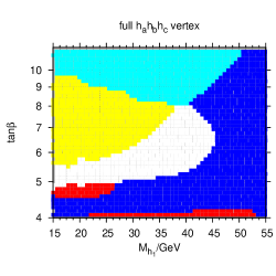
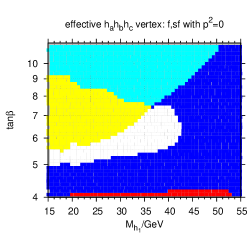
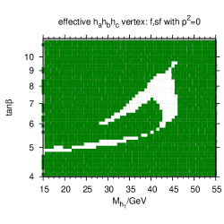
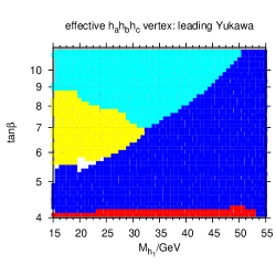
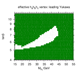
Figure 23: The channels with the highest statistical sensitivity (left) and LEP exclusion regions (right) for the CPX scenario at low values of $M_{h_{1}}$ and moderate values of $\tan\beta$. The top row shows a subset of the results shown in Fig. 21 and Fig. 22. In the second row, the genuine vertex corrections to the $h_{2}\to h_{1}h_{1}$ branching ratio include only the $f,\tilde{f}$ corrections at zero external momenta and, in the third row, the vertex corrections to the $h_{2}\to h_{1}h_{1}$ branching ratio have been calculated using the Yukawa approximation. In all three rows, the genuine vertex corrections to the $h_{2}\to h_{1}h_{1}$ branching ratio are combined with the full propagator corrections. Left: red = $h_{1}Z\to b\bar{b}Z\,({\color[rgb]{1,0,0}\blacksquare})$, blue = $h_{2}Z\to b\bar{b}Z\,({\color[rgb]{0,0,1}\blacksquare})$, white = $h_{2}Z\to h_{1}h_{1}Z\to b\bar{b}b\bar{b}Z\,(\square)$, cyan = $h_{2}h_{1}\to b\bar{b}b\bar{b}\,({\color[rgb]{0,1,1}\blacksquare})$, yellow = $h_{2}h_{1}\to h_{1}h_{1}h_{1}\to b\bar{b}b\bar{b}b\bar{b}\,({\color[rgb]{1,1,0}\blacksquare})$, green = $h_{3}h_{1}\to b\bar{b}b\bar{b}\,({\color[rgb]{0,1,0}\blacksquare})$, purple = other channels (${\color[rgb]{0,0,0}\blacksquare}$). Right: green (darker grey) = LEP excluded, white = LEP allowed.

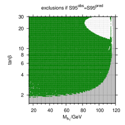
Figure 24: The LEP exclusion regions for the hypothetical case in which all of the observed cross section values were measured to be the same as the ones expected in a background-only simulation. The colour codings are: green (darker grey) = LEP excluded, white = LEP allowed.

In order to further investigate the effects of our new genuine vertex corrections to the $h_{2}\to h_{1}h_{1}$ decay, we now compare the LEP exclusion regions based on the full result with cases where we have used various approximations to calculate the genuine vertex corrections to the $h_{2}\to h_{1}h_{1}$ decay. In Fig. 23 (centre), the genuine vertex corrections are approximated by the $f,\tilde{f}$ corrections at zero external momenta. Fig. 23 (lower) displays the result when the leading Yukawa corrections to the triple Higgs vertex, as given by eqs. (6.1.1)–(97), are used.

The boundary between channels related to $|g^{{\rm eff}}_{h_{2}ZZ}|^{2}$ (i.e. $h_{2}Z\to h_{1}h_{1}Z\to b\bar{b}b\bar{b}Z\,(\square)$ and $h_{2}Z\to b\bar{b}Z\,({\color[rgb]{0,0,1}\blacksquare})$) and those related to $|g^{{\rm eff}}_{h_{2}h_{1}Z}|^{2}$ (i.e. $h_{2}h_{1}\to b\bar{b}b\bar{b}\,({\color[rgb]{0,1,1}\blacksquare})$ and $h_{2}h_{1}\to h_{1}h_{1}h_{1}\to b\bar{b}b\bar{b}b\bar{b}\,({\color[rgb]{1,1,0}\blacksquare})$) for both approximations are in about the same position as in Fig. 23 (upper). However, the boundaries between channels directly involving the $h_{2}\to h_{1}h_{1}$ decay and those that do not involve this decay have shifted. In particular, the region where the channel $h_{2}Z\to h_{1}h_{1}Z\to b\bar{b}b\bar{b}Z\,(\square)$ has the highest statistical sensitivity disappears entirely if the ‘leading Yukawa’ approximation is used. This has a considerable impact on the shape of the unexcluded region B. The $f,\tilde{f}$ at $p^{2}=0$ approximation, on the other hand, performs very well, yielding an unexcluded region B which, in position and shape, agrees very well with the full result.

Figure 25: The LEP exclusions for the CPX scenario plotted in the $M_{h_{1}}-\tan\beta$ plane. Results for $m_{t}=173.1+1.3\,\,\mathrm{GeV}$ and $m_{t}=173.1-1.3\,\,\mathrm{GeV}$. White: point is unexcluded in both, light green (lighter grey): point is excluded in only one, dark green (darker grey): point is excluded in both.

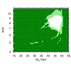
Figure 26: The LEP exclusions for the CPX scenario plotted in the $M_{h_{1}}-\tan\beta$ plane. Results for (a) $m_{t}^{OS}$ in the 2-loop corrections in Higgs self energies and $m_{t}^{OS}$ in the 1-loop genuine $h_{a}h_{b}h_{c}$ vertex corrections, and (b) $m_{t}^{\overline{\rm{MS}},SM}$ in the 2-loop corrections in Higgs self energies and $m_{t}^{\overline{\rm{MS}},SM}$ in the 1-loop genuine $h_{a}h_{b}h_{c}$ vertex corrections. White: point is unexcluded in both, light green (lighter grey): point is excluded in only one, dark green (darker grey): point is excluded in both.

It is interesting to consider the effect of the experimental uncertainty on the mass of the top quark. Since the leading corrections to the $h_{2}\to h_{1}h_{1}$ vertex are Yukawa corrections proportional to $m_{t}^{4}$, one would expect the unexcluded region B to exhibit a strong dependence on $m_{t}$. The neutral Higgs masses are also very sensitive to $m_{t}$, since these Yukawa corrections are also the leading corrections to the Higgs self-energies. We use the experimental value $m_{t}=173.1\pm 1.3\,\,\mathrm{GeV}$[64]. Fig. 25 shows the result of running scans for $m_{t}=173.1+1.3\,\,\mathrm{GeV}$ and $m_{t}=173.1-1.3\,\,\mathrm{GeV}$ over the area of $\rm{CPX}$ parameter space containing the unexcluded region B. Parameter points which are excluded at both top masses are shown as dark green (darker grey), those excluded at one of the masses only are in light green (lighter grey) and those which remain unexcluded at both masses are in white. Therefore, the light green area (lighter grey area) demonstrates the uncertainty on the size and shape of the unexcluded region B due to the uncertainty from the measurement of the top mass. The unexcluded area for $m_{t}=173.1+1.3\,\,\mathrm{GeV}$ is approximately double the size of the unexcluded area for $m_{t}=173.1-1.3\,\,\mathrm{GeV}$.

It is also possible to use a similar strategy to investigate the dependence of the size of the unexcluded region B on the choice of $m_{t}$ at the higher loop orders in the calculation. In Fig. 26, we use (a) $m_{t}^{OS}$ in the 2-loop corrections in Higgs self energies and $m_{t}^{OS}$ in the 1-loop genuine $h_{a}h_{b}h_{c}$ vertex corrections, and (b) $m_{t}^{\overline{\rm{MS}},SM}$ in the 2-loop corrections in Higgs self energies (as discussed in Sect. 5.4) and $m_{t}^{\overline{\rm{MS}},SM}$ in the 1-loop genuine $h_{a}h_{b}h_{c}$ vertex corrections (as previously). Points in parameter space which are excluded for the results of both calculation (a) and (b) are shown in dark green (darker grey), points excluded for the results of one calculation only are shown in light green (lighter grey), and points in white can be excluded for the results of neither calculation. In this way, we can get a rough estimate of the dependence of unexcluded region B on higher order corrections in the $t,\tilde{t}$ sector – whilst these corrections are significant, the existence of an unexcluded region in this part of CPX parameter space is confirmed in both. Note that the region in which the results of one of the two calculations yield an unexcluded region forks into two narrow regions at its base, rather than one, reflecting the different positioning of the boundaries between regions where different processes have the highest statistical sensitivity in the two analyses contributing to this exclusion plot.

The variation of $\phi_{A_{t}}$ has an interesting impact on the unexcluded regions. Recall that, in Fig. 10 (left), we saw that there was a peak in the $h_{2}\to h_{1}h_{1}$ decay width at moderate $\tan\beta$, and a minimum at lower $\tan\beta$. Varying $\phi_{A_{t}}$ by 10% has a dramatic effect on the decay width, through changing the magnitude and position of this peak and changing its position with respect to $\tan\beta$. In Fig. 27, which uses $\phi_{A_{t}}=0.9\times\pi/2$ and $\phi_{A_{t}}=1.1\times\pi/2$, we can see these effects reflected in the $h_{2}\to h_{1}h_{1}$ branching ratio. In particular, we see that the thin horizontal minimum in BR($h_{2}\to h_{1}h_{1}$) shifts to higher $\tan\beta$ as $\phi_{A_{t}}$ increases. We can also see a change in the shape of the region in which the $h_{2}\to h_{1}h_{1}$ decay is kinematically allowed and a slight change in the lower edge of CPX parameter space as plotted in the $M_{h_{1}}-\tan\beta$ plane.

As one would expect, this strong dependence of the $h_{2}\to h_{1}h_{1}$ branching ratio on $\phi_{A_{t}}$ is reflected in a change in the balance of the processes with the highest statistical sensitivity at each point in parameter space as $\phi_{A_{t}}$ increases. In particular, the size of the region in which either $h_{2}Z\to h_{1}h_{1}Z\to b\bar{b}b\bar{b}Z\,(\square)$ or $h_{2}h_{1}\to h_{1}h_{1}h_{1}\to b\bar{b}b\bar{b}b\bar{b}\,({\color[rgb]{1,1,0}\blacksquare})$ has the highest sensitivity decreases. The boundary between processes involving $|g^{{\rm eff}}_{h_{2}ZZ}|^{2}$ and those involving $|g^{{\rm eff}}_{h_{2}h_{1}Z}|^{2}$ also shifts to higher $\tan\beta$. As a result, the unexcluded region B occurs at higher $\tan\beta$ as $\phi_{A_{t}}$ increases and its shape changes significantly. The unexcluded region A increases in size as $\phi_{A_{t}}$ increases.

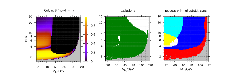
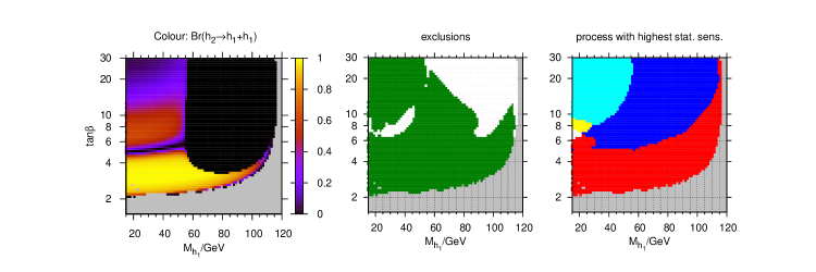
Figure 27: The $h_{2}\to h_{1}h_{1}$ branching ratio, LEP exclusions and channels with the highest statistical sensitivity plotted in the $M_{h_{1}}-\tan\beta$ plane. Upper graphs show $\phi_{A_{t}}=0.9\times\pi/2$, lower graphs show $\phi_{A_{t}}=1.1\times\pi/2$, other parameters taken from CPX scenario. See the captions of Fig. 21 and Fig. 22 for the colour codes of the plots in the second and third columns.

Fig. 28 illustrates that varying $|A_{t}|$ by 10% has a very substantial effect on the LEP exclusions in the CPX parameter space. Increasing $|A_{t}|$ has a large effect on the $h_{2}\to h_{1}h_{1}$ decay width. It increases the size of the peak at moderate $\tan\beta$ in Fig. 10 (left) and shifts the position of the minimum and the peak shown in Fig. 10 (left) to higher values of $\tan\beta$. Increasing $|A_{t}|$ also make the slope of this graph less steep above $\tan\beta\sim 7$. We see these effects reflected in the $h_{2}\to h_{1}h_{1}$ branching ratio in Fig. 28. We also see that a higher value of $|A_{t}|$ yields a significant increase in the area of parameter space in which the $h_{2}\to h_{1}h_{1}$ decay is kinematically allowed.

For the case in which $|A_{t}|=1.1\times 900\,\,\mathrm{GeV}$, the plot illustrating the channels with the highest statistical sensitivity in Fig. 28 is very different from those discussed so far. This is partly because $|g^{{\rm eff}}_{h_{1}h_{2}Z}|^{2}$ is reduced, which drastically reduces the area where $h_{2}h_{1}\to b\bar{b}b\bar{b}\,({\color[rgb]{0,1,1}\blacksquare})$ has the highest statistical sensitivity. The area where the channel $h_{2}h_{1}\to h_{1}h_{1}h_{1}\to b\bar{b}b\bar{b}b\bar{b}\,({\color[rgb]{1,1,0}\blacksquare})$ has the highest statistical sensitivity occurs at higher $\tan\beta$ than previously and is now unexcluded. Also, the suppression of $|g^{{\rm eff}}_{h_{1}h_{2}Z}|^{2}$ means that the channel $h_{3}h_{1}\to b\bar{b}b\bar{b}\,({\color[rgb]{0,1,0}\blacksquare})$ has the highest statistical sensitivity over a large region, which can only be partially excluded by this LEP limit. Therefore, the excluded LEP regions are dramatically different for the CPX scenario with $|A_{t}|=1.1\times 900\,\,\mathrm{GeV}$. It is worth noting, however, that this value of $|A_{t}|$ is close to an unstable region of parameter space, in which loop corrections in Higgs sector get extremely large. On the other hand, at $|A_{t}|=0.9\times 900\,\,\mathrm{GeV}$, the unexcluded region B has almost disappeared and the unexcluded region A has reduced in size as it is partially covered by two vertical excluded regions, at $M_{h_{1}}\sim 80\,\,\mathrm{GeV}$ and $M_{h_{1}}\sim 110\,\,\mathrm{GeV}$.

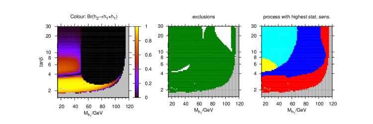
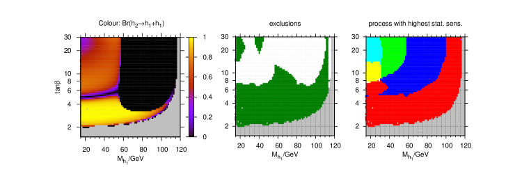
Figure 28: The $h_{2}\to h_{1}h_{1}$ branching ratio, LEP exclusions and channels with the highest statistical sensitivity plotted in the $M_{h_{1}}-\tan\beta$ plane. Upper graphs show $|A_{t}|=0.9\times 900\,\,\mathrm{GeV}$, lower graphs show $|A_{t}|=1.1\times 900\,\,\mathrm{GeV}$, other parameters taken from CPX scenario. See the captions of Fig. 21 and Fig. 22 for the colour codes of the plots in the second and third columns.

The gluino mass parameter $M_{3}$ does not feature in the 1-loop corrections to the $h_{2}\to h_{1}h_{1}$ decay or the 1-loop corrections to the Higgs masses. However, as we have seen, it can heavily influence the $h_{a}\to b\bar{b}$ decay width. In addition, the Higgs self-energies from FeynHiggs depend on $M_{3}$ through the $\mathcal{O}(\alpha_{t}\alpha_{s})$ corrections and the $\Delta m_{b}$ corrections. Therefore, it is interesting to see if varying this parameter has a significant effect on the LEP exclusions.

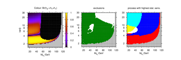
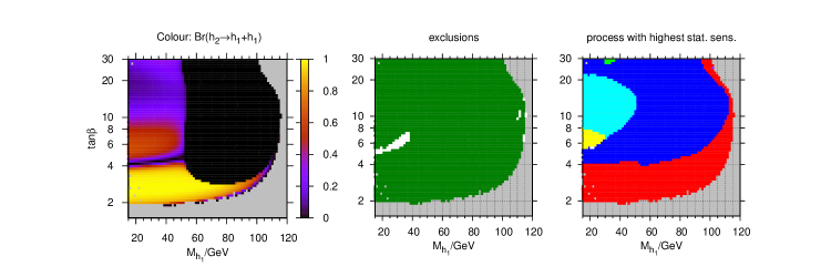
Figure 29: The $h_{2}\to h_{1}h_{1}$ branching ratio, LEP exclusions and channels with the highest statistical sensitivity plotted in the $M_{h_{1}}-\tan\beta$ plane. Upper graphs show $\phi_{M_{3}}=\pi/4$, lower graphs show $\phi_{M_{3}}=3\pi/4$, other parameters taken from CPX scenario. See the captions of Fig. 21 and Fig. 22 for the colour codes of the plots in the second and third columns.

In Fig. 29, we show results for $\phi_{M_{3}}=\pi/4$ and $\phi_{M_{3}}=3\pi/4$. At $\phi_{M_{3}}=\pi/4$, the area of the unexcluded regions A and B increases slightly compared to the CPX setting of $\phi_{M_{3}}=\pi/2$. In contrast, at $\phi_{M_{3}}=3\pi/4$, the size of the unexcluded area B decreases and the unexcluded area A almost disappears. Note that the parameter space is not populated above $M_{h_{1}}\sim 100\,\,\mathrm{GeV}$ at $\tan\beta=30$.

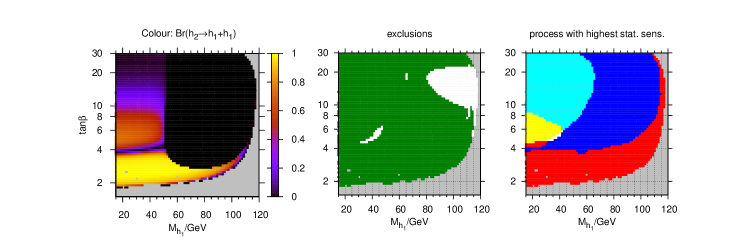
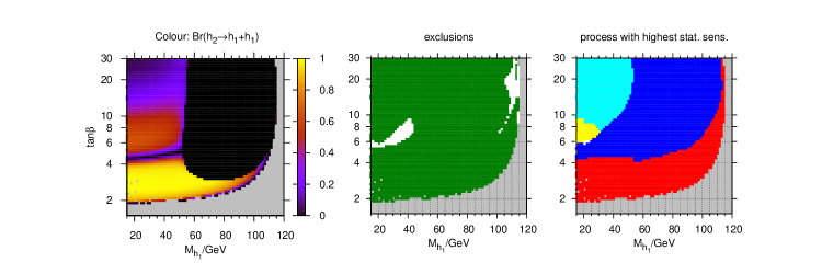
Figure 30: The $h_{2}\to h_{1}h_{1}$ branching ratio, LEP exclusions and channels with the highest statistical sensitivity plotted in the $M_{h_{1}}-\tan\beta$ plane. Upper graphs show $|M_{3}|=100\,\,\mathrm{GeV}$, lower graphs show $|M_{3}|=2000\,\,\mathrm{GeV}$, other parameters taken from CPX scenario. See the captions of Fig. 21 and Fig. 22 for the colour codes of the plots in the second and third columns.

Fig. 30 illustrates the results for $|M_{3}|=100\,\,\mathrm{GeV}$ and $|M_{3}|=2000\,\,\mathrm{GeV}$. Both unexcluded regions are reduced in both cases. Note that, for $|M_{3}|=100\,\,\mathrm{GeV}$, the excluded region A is bounded from above.

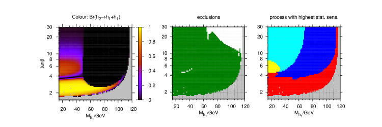
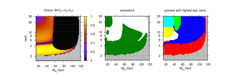
Figure 31: The $h_{2}\to h_{1}h_{1}$ branching ratio, LEP exclusions and channels with the highest statistical sensitivity plotted in the $M_{h_{1}}-\tan\beta$ plane. Upper graphs show $\mu=0.9\times 2000\,\,\mathrm{GeV}$, lower graphs show $\mu=1.1\times 2000\,\,\mathrm{GeV}$, other parameters taken from CPX scenario. See the captions of Fig. 21 and Fig. 22 for the colour codes of the plots in the second and third columns.

It is also interesting to consider the effect of varying the Higgsino mass parameter $\mu$. The branching ratios shown in Fig. 31 are qualitatively very similar to those in Fig. 28. As $\mu$ increases, $|g^{{\rm eff}}_{h_{2}ZZ}|^{2}$ is enhanced at the expense of $|g^{{\rm eff}}_{h_{2}h_{1}Z}|^{2}$, and this determines the relative sizes of the regions involving these couplings. The plot with $\mu=1.1\times 2000\,\,\mathrm{GeV}$ in Fig. 31 has a large region in which the channel $h_{2}Z\to h_{1}h_{1}Z\to b\bar{b}b\bar{b}Z\,(\square)$ has the highest statistical sensitivity. The unexcluded regions have increased in size substantially as $\mu$ increases and they have joined up.

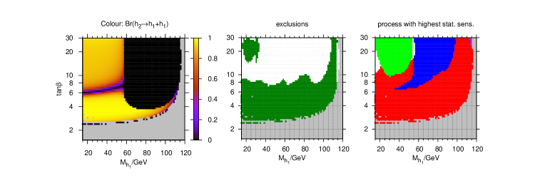
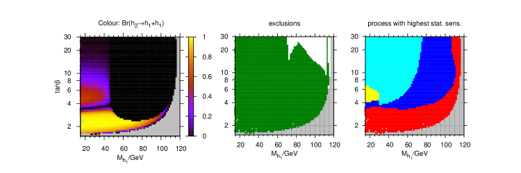
Figure 32: The $h_{2}\to h_{1}h_{1}$ branching ratio, LEP exclusions and channels with the highest statistical sensitivity plotted in the $M_{h_{1}}-\tan\beta$ plane. Upper graphs show $M_{\rm SUSY}=0.9\times 500\,\,\mathrm{GeV}$, lower graphs show $M_{\rm SUSY}=1.1\times 500\,\,\mathrm{GeV}$, other parameters taken from CPX scenario. See the captions of Fig. 21 and Fig. 22 for the colour codes of the plots in the second and third columns.

Similarly, the effect of decreasing the soft-breaking term $M_{\rm SUSY}$ by 10%, as shown in Fig. 32, can be explained by an enhancement of $|g^{{\rm eff}}_{h_{2}ZZ}|^{2}$ at the expense of $|g^{{\rm eff}}_{h_{2}h_{1}Z}|^{2}$ and a suppression of BR($h_{2}\to b\bar{b}$) as $M_{\rm SUSY}$ decreases. This results in a very large unexcluded region, covering the majority of the parameter space above $\tan\beta\sim 9$. In contrast, increasing the value of $M_{\rm SUSY}$ to $M_{\rm SUSY}=1.1\times 500\,\,\mathrm{GeV}$ greatly reduces the amount of unexcluded parameter space. In addition, note that the parameter space is populated at lower values of $\tan\beta$ at this value of $M_{\rm SUSY}$.

10.3 Comparison with CPsuperH

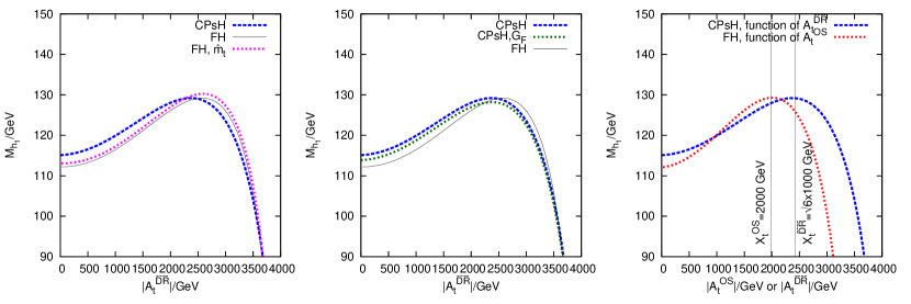
(a)                                           (b)                                           (c)

Figure 33: Lightest neutral Higgs mass as a function of $A^{\overline{\rm{DR}}}_{t}$ in the $m_{h}^{\rm max}$ scenario, with $\tan\beta=10$, $M_{H^{\pm}}=1000\,\,\mathrm{GeV}$. All FeynHiggs results shown here use the full Higgs self-energies, and the $\overline{\rm{DR}}$ to on-shell parameter conversion involves terms at both $\mathcal{O}(\alpha_{s})$ and $\mathcal{O}(\alpha_{t})$, and the calculation is parametrised in terms of $m^{OS}_{t}$ unless otherwise stated.
(a) blue dashed: CPsuperH, black solid: FeynHiggs, magenta dotted: FeynHiggs with code edited such that calculation is parametrised in terms of $\overline{m}_{t}$.
(b) blue dashed: CPsuperH, green dotted: CPsuperH but with the result parametrised in terms of the Fermi constant instead of $\alpha(M_{Z})$, black solid: FeynHiggs.
(c) blue dashed: CPsuperH as a function of $A_{t}^{\overline{\rm{DR}}}$ as before, red dotted: FeynHiggs as a function of $A_{t}^{OS}$.

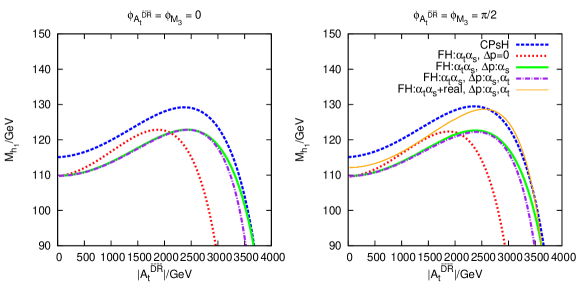
Figure 34: Lightest neutral Higgs mass as a function of $A_{t}^{\overline{\rm{DR}}}$ in the $m_{h}^{\rm max}$ scenario (left) and a CP-violating $m_{h}^{\rm max}$-like scenario (right), where $\phi_{A_{t}^{\overline{\rm{DR}}}}=\phi_{M_{3}}=\pi/2$. In both plots, $\tan\beta=10$ and $M_{H^{\pm}}=1000\,\,\mathrm{GeV}$. All FeynHiggs results use Higgs self-energies up to $\mathcal{O}(\alpha_{t}\alpha_{s})$ only (with the exception of the orange (thin solid) line) and the calculation is parametrised in terms of $m^{OS}_{t}$. Blue dashed: CPsuperH as in Fig. 33, red dotted: FeynHiggs result without parameter shifts for the input parameters i.e.  $\Delta p=0$, green solid (thick): FeynHiggs with $\Delta p$ at $\mathcal{O}(\alpha_{s})$, purple dot-dashed: FeynHiggs result with $\Delta p$ involving contributions at $\mathcal{O}(\alpha_{s})$ and $\mathcal{O}(\alpha_{t})$, orange solid (thin): as for purple, except subleading 2-loop corrections are included in the Higgs self-energies, calculated at all possible combinations of $\phi_{X_{t}}=0,\pi$, $\phi_{X_{b}}=0,\pi$ and $\phi_{M_{3}}=0,\pi$. Therefore, there are eight orange lines in total, but they lie too close to each other to be distinguishable by eye.

As we discussed in Sect. 5, when comparing our calculation with the results from CPsuperH, we need to make sure that we account for the difference between the definitions of the input parameters.

When comparing LEP exclusion plots, we shall investigate both the $\overline{\rm{CPX}}$ and $\rm{CPX}$ scenarios, as defined in Sect. 3 (recall that, in the $\overline{\rm{CPX}}$ scenario, the input parameters $A_{t}$, $M_{L}^{2}$ and $M_{\tilde{t}R}^{2}$ are defined in the $\overline{\rm{DR}}$ scheme, while in the $\rm{CPX}$ scenario, they are defined in the on-shell scheme). The $\overline{\rm{CPX}}$ scenario is used most frequently in the literature as an example of an interesting CP-violating MSSM scenario and closely resembles the CP-violating scenario used by the LEP Higgs Working Group [2]. The $\rm{CPX}$ scenario is a more natural scenario in which to perform a Feynman-diagrammatic calculation and therefore has been used throughout the majority of this paper, up to this section.

However, we shall begin the discussion by an investigation of two scenarios with less extreme parameter values than the $\overline{\rm{CPX}}$ and $\rm{CPX}$ scenarios, i.e. where the higher-order effects are expected to be smaller. We will use the (CP-conserving) $m_{h}^{\rm max}$ scenario, where we interpret the stop sector parameters $A_{t}$, $M_{L}$ and $M_{\tilde{t}R}$ as $\overline{\rm{DR}}$ parameters ($\tan\beta=10$, $M_{H^{\pm}}=M_{L}^{\overline{\rm{DR}}}(M_{S})=M^{\overline{\rm{DR}}}_{\tilde{t}R}(M_{S})=1000\,\,\mathrm{GeV}$, $\mu^{\overline{\rm{DR}}}(M_{S})=200\,\,\mathrm{GeV}$, $M_{3}=800\,\,\mathrm{GeV}$). We also consider an ‘$m_{h}^{\rm max}$-like’ scenario with CP violation (as for $m_{h}^{\rm max}$, but $\phi^{\overline{\rm{DR}}}_{A_{t}}=\phi^{\overline{\rm{DR}}}_{M_{3}}=\pi/2$). Since we have defined $A_{t}$, $M_{L}^{2}$, $M_{\tilde{t}R}^{2}$ and $\mu$ in the $\overline{\rm{DR}}$ renormalisation scheme at $M_{S}$, we must make use of the parameter conversions described in Sect. 5, in order to obtain $A_{t}^{\rm on-shell}$, $M_{L}^{\rm on-shell}$, $M_{\tilde{t}R}^{\rm on-shell}$ and $\mu^{\overline{\rm{DR}}}(m_{t})$, which are the input parameters that need to be given to FeynHiggs.

In Fig. 33 (a), we display the result from CPsuperH (blue dashed) and the result from FeynHiggs using $\mathcal{O}(\alpha_{s})$ and $\mathcal{O}(\alpha_{t})$ contributions to the parameter shifts (black solid) (as discussed in Sect. 5) in the $m_{h}^{\rm max}$ scenario. We can see that the maximum value of $M_{h_{1}}$ agrees to within $0.1\,\,\mathrm{GeV}$ between the two codes, although the maximum occurs at a value of $A_{t}^{\overline{\rm{DR}}}$ which is $\sim 200\,\,\mathrm{GeV}$ higher for the FeynHiggs result than the CPsuperH result. Note also that there is a somewhat larger discrepancy between the two codes at small values of $A_{t}^{\overline{\rm{DR}}}$, where CPsuperH predicts a mass $\sim 3\,\,\mathrm{GeV}$ higher than FeynHiggs. Since FeynHiggs contains the full $\mathcal{O}(\alpha_{t}\alpha_{s})$, $\mathcal{O}(\alpha_{t}^{2})$ and the complete 1-loop corrections to the neutral Higgs self-energies in the MSSM with real parameters, while CPsuperH only contains the leading logarithmic contributions, we should not expect our $\mathcal{O}(\alpha_{s})$ and $\mathcal{O}(\alpha_{t})$ parameter shifts to convert perfectly between the two calculations.

Also shown in Fig. 33 (a) is the result where the FeynHiggs calculation is parametrised in terms of the $\overline{\rm{MS}}$ top mass (magenta dotted), as discussed in Sect. 5.4, instead of the on-shell top mass (black solid). This changes the Higgs mass by less than $2\,\,\mathrm{GeV}$ (for $A_{t}^{\overline{\rm{DR}}}<3600\,\,\mathrm{GeV}$), which is appropriately small since this is formally a higher order effect.

Another contribution to the remaining discrepancy between the results for the Higgs mass predictions in the two codes is the difference in the way that the electric charge is parameterised at lowest order in the two codes. We investigate the magnitude of this effect in the following way. The input to CPsuperH is supposed to be $\alpha(M_{Z})$ (blue dashed), but we can investigate the effect of changing it to $\alpha\to G_{F}2\sqrt{2}M_{W}^{2}s_{W}^{2}/(4\pi)$ (green dotted), which should only affect the calculation at the level of the unknown higher order contributions. In Fig. 33 (b), we can see that this changes the lightest Higgs mass by less than $1.3\,\,\mathrm{GeV}$ for $A_{t}^{\overline{\rm{DR}}}<3600\,\,\mathrm{GeV}$.

A meaningful comparison between the two Higgs mass calculations can also be carried out in the $m_{h}^{\rm max}$ scenario by neglecting the parameter shifts in $M_{L}$ and $M_{\tilde{t}R}$ and using the values of $X_{t}^{OS}$ and $X_{t}^{\overline{\rm{DR}}}$, which maximise the lightest Higgs masses from FeynHiggs and CPsuperH, respectively (corresponding to independently defining a $m_{h}^{\rm max}$ scenario in the on-shell scheme and a $m_{h}^{\rm max}$ scenario in the $\overline{\rm{DR}}$ scheme). Using the leading 1-loop and 2-loop corrections, it is possible to predict that this will occur at approximately $X_{t}^{OS}=2000\,\,\mathrm{GeV}$ and $X_{t}^{\overline{\rm{DR}}}=\sqrt{6}\times 1000\,\,\mathrm{GeV}$, see Ref. [77]. In Fig. 33 (c), we plot the CPsuperH result for $M_{h_{1}}$ against $A_{t}^{\overline{\rm{DR}}}$ (blue dashed, as before), together with the FeynHiggs result for $M_{h_{1}}$ against $A_{t}^{OS}$ (red dotted). The maxima in $M_{h_{1}}$ occur at the points $(X_{t}^{OS},M_{h_{1}})=(1990\,\,\mathrm{GeV},129.3\,\,\mathrm{GeV})$ and $(X_{t}^{\overline{\rm{DR}}},M_{h_{1}})=(2350\,\,\mathrm{GeV},129.2\,\,\mathrm{GeV})$, i.e.  this definition of the $m_{h}^{\rm max}$ scenario does indeed give remarkable agreement between the two codes for the value of $M_{h_{1}}$. The two vertical lines show $X_{t}^{OS}=2000\,\,\mathrm{GeV}$ and $X_{t}^{\overline{\rm{DR}}}=\sqrt{6}\times 1000\,\,\mathrm{GeV}$ (we can see that using these approximate values of $X_{t}^{OS}$ and $X_{t}^{\overline{\rm{DR}}}$ predicts lightest Higgs masses which are within $0.1\,\,\mathrm{GeV}$ of the true values at the maxima).

It is interesting to compare the corresponding shift in $A_{t}$ i.e.  $\widetilde{\Delta}A_{t}=\widetilde{\Delta}X_{t}=X_{t}^{\overline{\rm{DR}}}-X_{t}^{OS}=2350-1990=360\,\,\mathrm{GeV}$, with the shift $\Delta A_{t}$ which we obtain from performing the parameter conversion. At $X_{t}^{\overline{\rm{DR}}}=\sqrt{6}\times 1000\,\,\mathrm{GeV}$, $\Delta A_{t}=510\,\,\mathrm{GeV}$ when just $\mathcal{O}(\alpha_{s})$ corrections are included in the parameter conversion and $\Delta A_{t}=600\,\,\mathrm{GeV}$ when both $\mathcal{O}(\alpha_{s})$ and $\mathcal{O}(\alpha_{t})$ corrections are included. Comparison with the analysis in Ref. [77], which was performed for the leading 1-loop and 2-loop contributions, shows a similar behaviour if only the $\mathcal{O}(\alpha_{s})$ correction to the parameter conversion is taken into account. Incorporating also the $\mathcal{O}(\alpha_{t})$ correction turns out to give rise to a slightly larger discrepancy between the shifts $\widetilde{\Delta}A_{t}$ and $\Delta A_{t}$. The numerical effect on the lightest Higgs mass, however, is small over this range of $A_{t}$.

As discussed in Sect. 4, the only 2-loop pieces contained within FeynHiggs which have been calculated with explicit phase dependence are of $\mathcal{O}(\alpha_{t}\alpha_{s})$. Before we start to discuss the CP-violating MSSM, it is instructive to compare the results from CPsuperH with the results given by FeynHiggs when the only 2-loop pieces which are included are $\mathcal{O}(\alpha_{t}\alpha_{s})$. This is shown in Fig. 34 (left). Also shown are the FeynHiggs results when the parameter shifts are neglected (red dotted), in order to give an idea of the size of the parameter shifts. We have a choice for the parameter shifts: we can either use the shifts at both $\mathcal{O}(\alpha_{s})$ and $\mathcal{O}(\alpha_{t})$ (purple dot-dashed) as before, or restrict to $\mathcal{O}(\alpha_{s})$ pieces (green solid (thick)). Theoretically, restricting to $\mathcal{O}(\alpha_{s})$ pieces (green solid (thick)) is preferable, since neither Higgs mass calculation now involves the full set of $\mathcal{O}(\alpha_{t}^{2})$ corrections. It can be seen that this choice makes very little difference in this scenario. We can see that, when we restrict to 2-loop pieces at $\mathcal{O}(\alpha_{t}\alpha_{s})$ in FeynHiggs, the resulting Higgs mass at the peak in the plot is approximately $7\,\,\mathrm{GeV}$ lighter than when all available corrections in FeynHiggs are used (and therefore also significantly lighter than the mass given by CPsuperH at the peak). In Fig. 34 (right), we introduce CP violation: this figure has the same parameters as Fig. 34 (left) ($\tan\beta=10$, $M_{H^{\pm}}=M_{L}^{\overline{\rm{DR}}}(M_{S})=M^{\overline{\rm{DR}}}_{\tilde{t}R}(M_{S})=1000\,\,\mathrm{GeV}$, $\mu^{\overline{\rm{DR}}}(M_{S})=200\,\,\mathrm{GeV}$, $|M_{3}|=800\,\,\mathrm{GeV}$), except that $A_{t}$, $A_{b}$ and $M_{3}$ are now complex: $\phi_{A_{t}^{\overline{\rm{DR}}}}=\phi_{A_{b}}=\phi_{M_{3}}=\pi/2$. Note that both the $\mathcal{O}(\alpha_{s})$ and $\mathcal{O}(\alpha_{t})$ parameter shifts include the full phase dependence, as described in Sect. 5. We can see that, in this scenario, the introduction of complex phases does not significantly affect the lightest Higgs mass. Therefore, we can deduce that the dominant source of the discrepancy between the masses in this CP-violating example are the neglected 2-loop corrections. It is instructive to consider whether the calculation of these 2-loop corrections to the neutral Higgs self-energies for the MSSM with real parameters can be used to give an estimate of these corrections in the complex MSSM. It is possible to evaluate these additional corrections at a phase of $0$ and $\pi$ for each complex parameter and then perform an interpolation between these results (this is an optional feature in FeynHiggs). In Fig. 34 (right), we show predictions for the lightest Higgs mass (orange solid (thin)) in the $\rm{CPX}$ scenario when the neutral Higgs self-energies are calculated up to $\mathcal{O}(\alpha_{t}\alpha_{s})$ with full phase dependence (as previously) and the subleading 2-loop corrections are calculated at combinations of $\phi_{X_{t}}=0,\pi$, $\phi_{X_{b}}=0,\pi$ and $\phi_{M_{3}}=0,\pi$. These eight combinations give very similar results, and their curves can not be distinguished in the plot, and, obviously, an interpolation between these results would also lie on this same line. It is, however, difficult to evaluate the accuracy of this Higgs mass prediction. On the one hand, it provides better agreement with the CPsuperH result, and the fact that the eight CP-conserving limits give very similar results could be interpreted as an indication that a fully phase-dependent calculation of these corrections may have only a mild dependence on the phase. However, a confirmation of this interpretation would require the actual result of a fully phase-dependent calculation. In an ‘extreme’ scenario like the $\rm{CPX}$ scenario, which is close to unstable regions of parameter space, the evaluation of the combinations of real parameters needed as input for the interpolation can be problematic. In particular, higher-order contributions in the CP-conserving limit $\phi_{X_{t}}=0$ turn out to be unphysically large in the $\rm{CPX}$ scenario and cause the mass calculation to fail (to obtain a real and positive mass value, the limit $\phi_{A_{t}}=0$ must be used instead). Since we will now turn our attention to such ‘extreme’ examples, exhibiting very large higher order corrections, we shall restrict in these cases the Higgs self-energies calculation in the complex MSSM to $\mathcal{O}(\alpha_{t}\alpha_{s})$, as we have done throughout the rest of the paper.

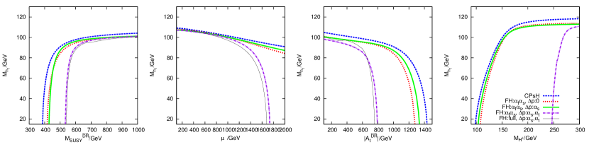
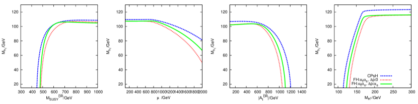
Figure 35: Lightest neutral Higgs mass in a CP-conserving version of the $\overline{\rm{CPX}}$ scenario at $\tan\beta=10,M_{H^{\pm}}=140\,\,\mathrm{GeV}$, as function of (left to right) $M_{SUSY}^{\overline{\rm{DR}}}(M_{S})$, $\mu^{\overline{\rm{DR}}}(M_{S})$, $|A_{t}^{\overline{\rm{DR}}}(M_{S})|$ and $M_{H^{\pm}}$. Blue dashed: CPsuperH result, red dotted: FeynHiggs with Higgs self-energies up to $\mathcal{O}(\alpha_{t}\alpha_{s})$, with $\Delta p=0$, green solid (thick): FeynHiggs with Higgs self-energies up to $\mathcal{O}(\alpha_{t}\alpha_{s})$ corrections, with $\Delta p$ at $\mathcal{O}(\alpha_{s})$, purple dot-dashed: FeynHiggs with Higgs self-energies up to $\mathcal{O}(\alpha_{t}\alpha_{s})$ corrections, with $\Delta p$ at $\mathcal{O}(\alpha_{s})$ and $\mathcal{O}(\alpha_{t})$, black solid (thin): FeynHiggs with full Higgs self-energies, with $\Delta p$ at $\mathcal{O}(\alpha_{s})$ and $\mathcal{O}(\alpha_{t})$.

Figure 36: Lightest neutral Higgs mass in the $\overline{\rm{CPX}}$ scenario at $\tan\beta=10,M_{H^{\pm}}=140\,\,\mathrm{GeV}$, as function of (left to right) $M_{SUSY}^{\overline{\rm{DR}}}(M_{S})$, $\mu$, $|A_{t}^{\overline{\rm{DR}}}(M_{S})|$ and $M_{H^{\pm}}$. (See Fig. 36 for the definitions of the abbreviations labelling the different curves.)

We shall first consider a CP-conserving version of the $\overline{\rm{CPX}}$ scenario i.e. the $\overline{\rm{CPX}}$ scenario with all phases set to zero (and $\mu^{\overline{\rm{DR}}}(M_{S})=2000\,\,\mathrm{GeV}$), as this will exhibit the main characteristics of the $\overline{\rm{CPX}}$ scenario (and, since we have more available corrections in the MSSM with real parameters than the MSSM with complex parameters, it will be easier for us to investigate). In Fig. 36, we compare the CPsuperH result (blue dashed) to the full FeynHiggs result with $\Delta p$ at $\mathcal{O}(\alpha_{s})$ and $\mathcal{O}(\alpha_{t})$ (black solid (thin)), the FeynHiggs result with Higgs self-energies only up to $\mathcal{O}(\alpha_{t}\alpha_{s})$ and $\Delta p$ at $\mathcal{O}(\alpha_{s})$ and $\mathcal{O}(\alpha_{t})$ (purple dot-dashed), the FeynHiggs result with Higgs self-energies up to $\mathcal{O}(\alpha_{t}\alpha_{s})$ and $\Delta p$ only at $\mathcal{O}(\alpha_{s})$ (green solid (thick)). Note that, when the $\mathcal{O}(\alpha_{t})$ contributions to $\Delta p$ are included, this incorporates the conversion of $\mu^{\overline{\rm{DR}}}(M_{S})$ to $\mu^{\overline{\rm{DR}}}(m_{t})$, using eq. (64). Also illustrated is the FeynHiggs result when the parameter shifts are neglected (red dotted), in order to demonstrate the numerical effect of the parameter shifts. In each plot in Fig. 36, we can see that the effect of the parameter shifts at $\mathcal{O}(\alpha_{t})$ on the mass calculation becomes very large once the nominal values of this CP-conserving $\overline{\rm{CPX}}$-like scenario are approached ($M_{SUSY}^{\overline{\rm{DR}}}=500\,\,\mathrm{GeV}$, $\mu^{\overline{\rm{DR}}}=2000\,\,\mathrm{GeV}$, $A_{t}^{\overline{\rm{DR}}}=1000\,\,\mathrm{GeV}$, $M_{H^{\pm}}=140\,\,\mathrm{GeV}$). Indeed, for the nominal values of this scenario, the lightest on-shell stop mass is driven to imaginary values when both the $\mathcal{O}(\alpha_{s})$ and $\mathcal{O}(\alpha_{t})$ parameter shifts are used (purple dot-dashed and black solid (thin)). These unphysically large effects are an indication that this scenario is close to an unstable region, which causes instabilities in the parameter conversion (this could imply that it would be appropriate to explicitly decouple the heavier particles in the conversion to the $\overline{\rm{DR}}$ scheme). In order to avoid these instabilities, we will, in the following, restrict the parameter conversion to $\mathcal{O}(\alpha_{s})$. Application of this parameter conversion, in conjunction with 2-loop mass corrections at $\mathcal{O}(\alpha_{t}\alpha_{s})$ (green solid (thick)), yields a relatively good agreement between the FeynHiggs and CPsuperH results.

We observe the same quantitative behaviour when we switch on the CP-violating phases in this scenario (Fig. 36), and therefore we can use the knowledge gained from the CP-conserving version to help interpret these characteristics. Once again, we find that the parameter conversions at $\mathcal{O}(\alpha_{s})$ and $\mathcal{O}(\alpha_{t})$ result in unphysically large corrections to the lightest Higgs mass and therefore restrict the parameter conversion to $\mathcal{O}(\alpha_{s})$ (green solid), which compares relatively well to the CPsuperH result (blue dashed).

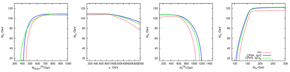
Figure 37: Lightest neutral Higgs mass in the $\rm{CPX}$ scenario at $\tan\beta=10,M_{H^{\pm}}=140\,\,\mathrm{GeV}$, as function of (left to right) $M_{SUSY}^{OS}$, $\mu$, $|A_{t}^{OS}|$ and $M_{H^{\pm}}$. Red dotted: FeynHiggs with Higgs self-energies up to $\mathcal{O}(\alpha_{t}\alpha_{s})$ corrections, blue dashed: CPsuperH with $\Delta p=0$, green dot-dashed: CPsuperH with $\Delta p$ at $\mathcal{O}(\alpha_{s})$,

We will now carry out a complementary analysis in the $\rm{CPX}$ scenario, which is defined in terms of on-shell stop sector parameters. Therefore, the parameter shifts are now used to convert from on-shell to $\overline{\rm{DR}}$ parameters, which can then be given as input to CPsuperH. Results for the lightest Higgs mass are shown in Fig. 37 for CPsuperH with no parameter conversion (blue dashed) and CPsuperH with parameter conversion at $\mathcal{O}(\alpha_{s})$ (green dot-dashed). Also shown is the FeynHiggs result where the masses are calculated at $\mathcal{O}(\alpha_{t}\alpha_{s})$ (red dotted). Once again, we can see that this scenario lies near the border of stable parameter space, which is necessary if we would like to investigate very low lightest Higgs masses. We find that, when the parameter conversion is performed in the on-shell to $\overline{\rm{DR}}$ direction, the effect of the parameter shifts tends to push the results into more stable regions of parameter space (rather than into more unstable regions, as it happens in the case of the $\overline{\rm{CPX}}$ scenario). However, we have confirmed that this parameter conversion still gives rise to large stop mass corrections at $\mathcal{O}(\alpha_{t})$.

Before starting a comparison of the LEP exclusions in $\overline{\rm{CPX}}$ or $\rm{CPX}$ parameter space, it is useful to describe the method that was used by the LEP Higgs Working Group to tackle this issue of consistently comparing results calculated in using different renormalisation schemes. The LHWG analysis was carried out in the $\overline{\rm{CPX}}$ scenario and both FeynHiggs version 2.0 [10] and CPH [5] (a predecessor of the program CPsuperH [11, 12]) were considered. The relation

$$\tilde{X}_{t}^{\rm CPH} = \tilde{X}_{t}+\frac{\alpha_{s}}{3\pi}M_{\rm SUSY}\left[8+\frac{4\tilde{X}_{t}}{M_{\rm SUSY}}-\frac{\pi\tilde{X}^{\rm FH}_{t}}{M_{\rm SUSY}}\log\left(\frac{m_{t}^{{\rm OS,}2}}{M^{2}_{\rm SUSY}}\right)\right]$$ (134)

was used [132] to convert between different definitions for $|A_{t}|$, with $\alpha_{s}=0.108$ and $\tilde{X}_{t}=|A_{t}|-\mu/\tan\beta$. The shifts in $\phi_{A_{t}}$ and $M_{\rm SUSY}(=M_{L}=M_{\tilde{t}_{R}})$ were neglected, and $A_{b}$ was set to be the same as $A_{t}$.

Near the region $M_{h_{1}}\sim 45\,\,\mathrm{GeV}$, $\tan\beta\sim 7$, this approximation gives a larger shift in $|A_{t}|$ than would be given from the full $\mathcal{O}(\alpha_{s})$ shifts, and therefore increases the agreement between the two Higgs mass codes. The LHWG then carried out two parallel analyses, one using Higgs sector predictions from CPH and one using Higgs sector predictions from FeynHiggs (apart from the triple Higgs coupling, as discussed in Sect. 10). Since they found significant differences between the two results, they considered a point in $\overline{\rm{CPX}}$ parameter space to be excluded only if it could be excluded in both the analysis based on the CPH results and the analysis based on the FeynHiggs results.

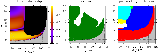
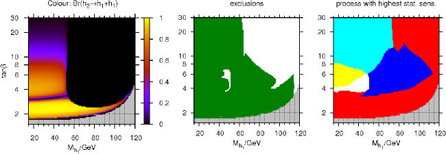
Figure 38: The $h_{2}\to h_{1}h_{1}$ branching ratio, LEP exclusions and channels with the highest statistical sensitivity for the $\overline{\rm{CPX}}$ scenario, plotted in the $M_{h_{1}}-\tan\beta$ plane. Top row: Using the calculations presented in this paper, parameter conversions at $\mathcal{O}(\alpha_{s})$ as described by eqs. (54)–(59), and neutral Higgs self-energies from FeynHiggs up to $\mathcal{O}(\alpha_{t}\alpha_{s})$. Bottom row: Using Higgs masses, couplings and branching ratios calculated by CPsuperH [11, 12]. See the captions of Fig. 21 and Fig. 22 for the colour codes of the plots in the second and third columns.

In Fig. 38 (top row), we use the topological cross section limits from LEP in conjunction with updated results for the Higgs masses, couplings and branching ratios, in the $\overline{\rm{CPX}}$ scenario using the parameter conversions at $\mathcal{O}(\alpha_{s})$. In particular, we use our complete 1-loop diagrammatic calculation for the $h_{i}\to h_{j}h_{k}$ decay processes with full phase dependence as described in Sect. 6 and we use renormalised neutral Higgs self-energies obtained from FeynHiggs (which includes corrections at $\mathcal{O}(\alpha_{t}\alpha_{s})$ with full phase dependence). We compare this to the results using the Higgs masses, couplings and branching ratios from the program CPsuperH, shown in Fig. 38 (bottom row). The CPsuperH prediction for the $h_{2}\to h_{1}h_{1}$ branching ratio is qualitatively similar to our result, although the thin ‘knife-edge’ region is at $\tan\beta\sim 3$ rather than $\tan\beta\sim 4.5$ and the peak at moderate $\tan\beta$ is higher but narrower, in particular, around $M_{h_{1}}\sim 45\,\,\mathrm{GeV}$. Also, different processes have the highest statistical sensitivity at different parts of the parameter space (Fig. 38 right column). Most significantly, the area where the process $h_{2}Z\to b\bar{b}Z\,({\color[rgb]{0,0,1}\blacksquare})$ has the highest statistical sensitivity is larger when using the Higgs sector predictions outlined in this paper, rather than the predictions given by CPsuperH. As a result, the unexcluded part of parameter space is much larger for $M_{h_{1}}<60\,\,\mathrm{GeV}$ when using our calculation and the unexcluded regions join together. However, for $M_{h_{1}}>60\,\,\mathrm{GeV}$, the unexcluded area is larger when the CPsuperH results are used.

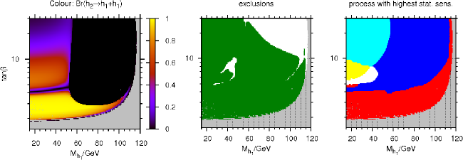
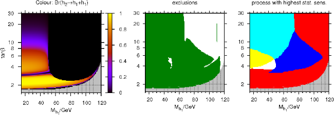
Figure 39: The $h_{2}\to h_{1}h_{1}$ branching ratio, LEP exclusions and channels with the highest statistical sensitivity for the $\rm{CPX}$ scenario, plotted in the $M_{h_{1}}-\tan\beta$ plane. Top row: Using the calculations presented in this paper and neutral Higgs self-energies from FeynHiggs up to $\mathcal{O}(\alpha_{t}\alpha_{s})$. Bottom row: Using Higgs masses, couplings and branching ratios calculated by CPsuperH [11, 12] and parameter conversions at $\mathcal{O}(\alpha_{s})$ as described by eqs. (54)–(59). See the captions of Fig. 21 and Fig. 22 for the colour codes of the plots in the second and third columns.

Finally, in Fig. 39, we compare the results from CPsuperH and our calculation (as shown previously in Fig. 16 (left), Fig. 21 (right) and Fig. 22 (right)) for the Higgs cascade decay width and LEP exclusions in the $\rm{CPX}$ scenario (defined in terms of on-shell stop sector parameters). Again, the CPsuperH prediction for the $h_{2}\to h_{1}h_{1}$ branching ratio is qualitatively similar to our result, although, once again, the thin ‘knife-edge’ region is at lower $\tan\beta$ and the maximum at moderate $\tan\beta$ is higher. As we saw in Fig. 38, the CPsuperH result has a large region where $h_{1}Z\to b\bar{b}Z\,({\color[rgb]{1,0,0}\blacksquare})$ has the highest statistical sensitivity at medium-to-high $\tan\beta$ and $M_{h_{1}}$, which is not seen in our result. Once again, the area where processes involving $h_{1}h_{2}$ pair-production (${\color[rgb]{0,1,1}\blacksquare}$ and ${\color[rgb]{1,1,0}\blacksquare}$) have the highest statistical sensitivity is larger in the CPsuperH result than in ours. As a result, the region where $h_{2}Z\to b\bar{b}Z\,({\color[rgb]{0,0,1}\blacksquare})$ has the highest statistical sensitivity does not significantly overlap with the region with large $h_{2}\to h_{1}h_{1}$ branching ratio, and therefore the region $M_{h_{1}}<65\,\,\mathrm{GeV}$ is almost entirely excluded. However, once again, the CPsuperH result has a larger unexcluded region at medium-to-high $\tan\beta$ and $M_{h_{1}}$.

In summary, we have compared the results presented in this paper with those given by the program CPsuperH. Since these results are very sensitive to the Higgs masses, we started with a comparison between the masses given by FeynHiggs and CPsuperH (including appropriate parameter transformations, which we have extended to the complex MSSM) in the $m_{h}^{\rm max}$ scenario, in a $m_{h}^{\rm max}$-like scenario with added CP violation, the $\overline{\rm{CPX}}$ scenario (in which the stop sector parameters have $\overline{\rm{DR}}$ definitions), the $\overline{\rm{CPX}}$ scenario with vanishing phases, and the $\rm{CPX}$ scenario (in which the stop sector parameters have on-shell definitions). We find good agreement between the mass calculations in the $m_{h}^{\rm max}$ and $m_{h}^{\rm max}$-like scenarios once the appropriate parameter shifts are taken into account. The $\overline{\rm{CPX}}$ scenario has been used by the LEP Higgs Working Group in their analysis and is the most frequently used CP-violating scenario in the literature. We find that the $\mathcal{O}(\alpha_{t})$ corrections in the parameter transformations for the stop masses are very large in this scenario and drive the $\tilde{t}_{1}$ mass to unphysical values. We interpret this as an indication that this scenario is close to an unstable region of parameter space (i.e.  a region with relatively large higher-order corrections), where we must be careful to avoid unphysically large corrections in the parameter shifts (which may require to explicitly decouple heavy particles in the conversion). When restricting to the $\mathcal{O}(\alpha_{s})$ parameter conversions, we find rough agreement between the mass predictions, and we observed similar behaviour when we considered the $\rm{CPX}$ scenario with appropriate parameter conversions at $\mathcal{O}(\alpha_{s})$. The variation in the Higgs sector predictions given by our calculation (using neutral Higgs self-energies from FeynHiggs) and CPsuperH are reflected in significant differences in the size and shape of the regions of parameter space that could not be excluded by the LEP results. When the topological cross section limits from LEP are confronted with the predictions of our calculation, significantly less parameter space can be excluded at low $M_{h_{1}}$. However, there is qualitative agreement about the existence of an unexcluded region at $M_{h_{1}}\sim 45\,\,\mathrm{GeV}$. Using either our calculation or the CPsuperH calculation results in large unexcluded regions at medium-to-high $\tan\beta$ and $M_{h_{1}}$. In general, more of the $\rm{CPX}$ parameter space can be excluded by LEP, as compared to the $\overline{\rm{CPX}}$ parameter space. Once again, both calculations are consistent with an unexcluded region at $M_{h_{1}}\sim 45\,\,\mathrm{GeV}$ in the $\rm{CPX}$ scenario, although, when CPsuperH Higgs sector predictions are used, this region is very small, and might be covered by a dedicated analysis of this scenario which could make use of a combination of different LEP Higgs search channels (as discussed in Sect. 10.2). However, both calculations once again yield large unexcluded regions of parameter space at medium-to-high $\tan\beta$ and $M_{h_{1}}$. Since the shape, size and position of the unexcluded regions vary significantly depending on which method was used to calculate the Higgs sector predictions, we adopt the LEP Higgs Working Group philosophy and only consider a point in parameter space excluded if it can be excluded using both methods independently. We therefore show these ‘combined’ exclusion plots in Fig. 40 for the $\overline{\rm{CPX}}$ and $\rm{CPX}$ scenarios. We conclude that there is still a sizeable area of parameter space in these scenarios below the kinematical limit at LEP which the LEP Higgs topological cross section limits are unable to exclude (in agreement with the LEP Higgs Working Group analysis) and therefore these scenarios with a very light neutral MSSM Higgs boson remain phenomenologically very interesting.

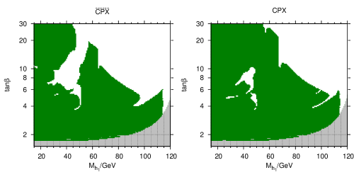
Figure 40: Combining results for the LEP exclusions in the $\overline{\rm{CPX}}$ (left, using Fig. 38) and $\rm{CPX}$ (right, using Fig. 39) parameter space. Green (darker grey): point in parameter space can be excluded using the topological LEP limits and the Higgs sector predictions from both our calculation (which uses neutral Higgs self-energies from FeynHiggs) and the calculation implemented into CPsuperH, white: is excluded by only one or by neither of the calculations.

11 Conclusions

In this paper we have presented theoretical predictions concerning the Higgs sector in the MSSM with complex parameters, which are especially relevant when considering MSSM scenarios that are particularly challenging for the past and present Higgs searches at LEP, the Tevatron and the LHC.

We have calculated the full 1-loop vertex corrections within the Feynman-diagrammatic approach for the process $h_{a}\to h_{b}h_{c}$, taking into account the dependence on all complex phases of the supersymmetric parameters and the full momentum dependence. We have included the full propagator corrections, using neutral Higgs self-energies as provided by FeynHiggs [6, 7, 8, 9, 10], and we have consistently included 1-loop mixing with the $Z$ boson and the unphysical Goldstone-boson degree of freedom. Our results are currently the most precise predictions for the $h_{a}\to h_{b}h_{c}$ decay width. These results will be included in the publicly available program FeynHiggs.

We have found that the genuine vertex corrections to the triple Higgs vertex are numerically very important. This holds both for the cases of CP conservation and CP violation. The inclusion of the genuine vertex corrections changes the predictions for the decay widths drastically as compared to an approximation based solely on propagator-type corrections. Using the leading Yukawa contributions or the full fermion/sfermion vertex corrections at zero incoming momentum yields a prediction for the decay width which is closer to the full result, but we still find deviations of $\sim 30\%$ and $\sim 15\%$, respectively, in the example of the CPX parameter space at $\tan\beta\sim 9$, $M_{h_{1}}\sim 40\,\,\mathrm{GeV}$. Yet, these approximations can be useful in terms of effective couplings. The Yukawa approximation including all leading corrections can be expressed in a very compact form, thus providing a convenient way to go beyond the tree level vertex contributions. The effective coupling created from the full fermion/sfermion contributions at vanishing external momentum is a more sophisticated effective coupling approximation. These effective couplings can be used for theoretical predictions of cross sections for processes such as $e^{+}e^{-}\to h_{1}Z\to h_{1}h_{1}Z$ at a future Linear Collider and the corresponding process at the LHC, which are of great interest in order to directly access the Higgs self-couplings and thus investigate a crucial element of the Higgs mechanism. We find that the genuine vertex corrections enhance the triple-Higgs squared coupling of the light CP-even Higgs boson of the MSSM by 20–60% in the phenomenologically relevant region as compared to the lowest order coupling in the Standard Model for the same value of the Higgs mass. This could have interesting implications for the sensitivity of searches at the LHC and a future Linear Collider to effects of the triple-Higgs coupling.

We also have presented the full 1-loop electroweak vertex corrections to the $h_{a}\to f\bar{f}$ decay width in the complex MSSM, including full phase dependence. We have supplemented these contributions with 1-loop QED and SM QCD corrections, resummed SUSY QCD contributions, propagator corrections calculated using neutral Higgs self-energies from FeynHiggs, and 1-loop propagator mixing with Goldstone bosons and Z bosons. Our calculation has already been incorporated into the program FeynHiggs.

We performed on-shell to $\overline{\rm{DR}}$ parameter conversions at $\mathcal{O}(\alpha_{s})$ and $\mathcal{O}(\alpha_{t})$ for the general case of complex supersymmetric parameters, to be used when comparing results of calculations based on different renormalisation schemes. We also present a simple approximation to the $\mathcal{O}(\alpha_{s})$ contribution to these parameter shifts, which is valid in the complex MSSM.

We investigated the numerical impact of parametrising the neutral Higgs self-energies (in the Feynman-diagrammatic approach) in terms of the $\overline{\rm{MS}}$ top mass, rather than the on-shell top mass, which is formally a 3-loop effect. This will be incorporated as a possible option in FeynHiggs.

Furthermore, the investigated $t,\tilde{t},b,\tilde{b}$ genuine vertex corrections to the LEP Higgsstrahlung and LEP pair production processes in the CP-violating MSSM were found to have a small numerical impact in the CPX parameter space.

Using our new theoretical predictions in conjunction with the topological cross section limits from the LEP Higgs searches (there exist no relevant limits for this parameter region from the Tevatron), we were able to investigate the effect of the new contributions on the exclusion regions in the CPX benchmark scenario. Of particular interest is the region $30\,\,\mathrm{GeV}\;\raisebox{-3.00003pt}{$\stackrel{{\scriptstyle\displaystyle<}}{{\sim}}$}\;M_{h_{1}}\;\raisebox{-3.00003pt}{$\stackrel{{\scriptstyle\displaystyle<}}{{\sim}}$}\;50\,\,\mathrm{GeV}$, $3\;\raisebox{-3.00003pt}{$\stackrel{{\scriptstyle\displaystyle<}}{{\sim}}$}\;\tan\beta\;\raisebox{-3.00003pt}{$\stackrel{{\scriptstyle\displaystyle<}}{{\sim}}$}\;10$, which previous analyses had not been able to exclude, despite the relatively low values of $M_{h_{1}}$ involved. Since the coupling of the lightest Higgs boson to gauge bosons is suppressed in much of this region, processes involving the second heaviest or the heaviest neutral Higgs boson are important. Across the majority of this region, the $h_{2}\to h_{1}h_{1}$ decay is dominant and therefore a precise theoretical prediction for this decay width is crucial for investigating whether an unexcluded region actually exists and for mapping out its extent. Our results confirm the existence of an unexcluded region at $M_{h_{1}}\sim 45\,\,\mathrm{GeV}$. Furthermore, we find that there is a rather large unexcluded region in the CPX-type scenarios below the LEP limit for a SM-like Higgs, occurring at medium to high values of $\tan\beta$ and extending down to $M_{h_{1}}$ values of about $60\,\,\mathrm{GeV}$. We have performed a detailed analysis of the dependence of the unexcluded parameter regions on variations of the MSSM parameters.

After discussing in detail the issues involved in such a comparison, we have compared our results for the impact of the existing Higgs search results on the parameter region of the CPX scenario with the results obtained using the publicly available program CPsuperH. While both analyses confirm the existence of unexcluded regions in similar parts of the CPX parameter space, sizable differences occur in the detailed extent of these regions.

Our results should serve as a motivation to focus Higgs searches at the LHC not only on the mass range above about $114\,\,\mathrm{GeV}$, corresponding to the allowed region for a SM-like Higgs, but to perform dedicated searches also for much lighter Higgs states.

12 Acknowledgements

We would like to thank Oliver Brein, Alison Fowler, Howard Haber, Thomas Hahn, Sven Heinemeyer, Wolfgang Hollik, David Lopez Val, Sophy Palmer and Pietro Slavich for valuable discussions and advice. Work supported in part by the Helmholtz Alliance HA-101 ’Physics at the Terascale’, the European Community’s Marie-Curie Research Training Network under contract MRTN-CT-2006-035505 ‘Tools and Precision Calculations for Physics Discoveries at Colliders’ (HEPTOOLS) and MRTN-CT-2006-035657 ‘Understanding the Electroweak Symmetry Breaking and the Origin of Mass using the First Data of ATLAS’ (ARTEMIS).

Appendix A Relations between $\Sigma_{h_{i}G}$ and $\Sigma_{h_{i}Z}$

Using a Feynman-diagrammatic calculation, we find that the following relations hold at 1-loop order in the $R_{\xi}$-gauge:

$$M_{Z}\Sigma_{\phi_{2}G}(p^{2})+ip^{2}\Sigma_{\phi_{2}Z}(p^{2}) = -\frac{e}{2c_{W}s_{W}}c_{\beta}t_{A},$$

$$M_{Z}\Sigma_{\phi_{1}G}(p^{2})+ip^{2}\Sigma_{\phi_{1}Z}(p^{2}) = \frac{e}{2c_{W}s_{W}}s_{\beta}t_{A},$$

$$M_{Z}\Sigma_{AG}(p^{2})+ip^{2}\Sigma_{AZ}(p^{2})+M_{Z}(p^{2}-m_{A}^{2})f_{0}(p^{2}) = \frac{e}{2c_{W}s_{W}}\left(c_{\beta}t_{\phi_{2}}-s_{\beta}t_{\phi_{1}}\right),$$

$$M_{Z}\Sigma_{GG}(p^{2})+2ip^{2}\Sigma_{GZ}(p^{2})-\frac{p^{2}}{M_{Z}}\Sigma^{L}_{ZZ}(p^{2}) = \frac{e}{2c_{W}s_{W}}\left(s_{\beta}t_{\phi_{2}}+c_{\beta}t_{\phi_{1}}\right),$$

$$M_{W}\Sigma_{H^{-}G^{+}}(p^{2})-p^{2}\Sigma_{H^{-}W^{+}}(p^{2})+M_{W}(p^{2}-m_{H^{\pm}}^{2})f_{\pm}(p^{2}) = \frac{e}{2s_{W}}\left(c_{\beta}t_{\phi_{2}}-s_{\beta}t_{\phi_{1}}+it_{A}\right),$$

$$M_{W}\Sigma_{G^{-}G^{+}}(p^{2})-2p^{2}\Sigma_{G^{-}W^{+}}(p^{2})-\frac{p^{2}}{M_{W}}\Sigma^{L}_{WW}(p^{2}) = \frac{e}{2s_{W}}\left(s_{\beta}t_{\phi_{2}}+c_{\beta}t_{\phi_{1}}\right),$$ (135)

where

$$f_{0}(p^{2}) = -\frac{\alpha}{16\pi s_{W}^{2}M_{W}^{2}}s_{\beta-\alpha}c_{\beta-\alpha}M_{Z}^{2}\xi_{Z}\left[B_{0}\left(p^{2},m_{h}^{2},M_{Z}^{2}\xi_{Z}\right)-B_{0}\left(p^{2},m_{H}^{2},M_{Z}^{2}\xi_{Z}\right)\right],$$ (136)

$$f_{\pm}(p^{2}) = -\frac{\alpha}{16\pi s_{W}^{2}M_{W}^{2}}s_{\beta-\alpha}c_{\beta-\alpha}M_{W}^{2}\xi_{W}\left[B_{0}\left(p^{2},m_{h}^{2},M_{W}^{2}\xi_{W}\right)-B_{0}\left(p^{2},m_{H}^{2},M_{W}^{2}\xi_{W}\right)\right].$$

$f_{0},f_{\pm}$ are finite and do not contribute if the particle is on-shell.

In terms of renormalised quantities, the relations are given by

$$\hat{\Sigma}_{hG}(p^{2})+\frac{ip^{2}}{M_{Z}}\hat{\Sigma}_{hZ}(p^{2}) = 0,$$ (138)

$$\hat{\Sigma}_{HG}(p^{2})+\frac{ip^{2}}{M_{Z}}\hat{\Sigma}_{HZ}(p^{2}) = 0,$$ (139)

$$\hat{\Sigma}_{AG}(p^{2})+\frac{ip^{2}}{M_{Z}}\hat{\Sigma}_{AZ}(p^{2})+(p^{2}-m_{A}^{2})f_{0}(p^{2}) = 0,$$ (140)

$$\hat{\Sigma}_{GG}(p^{2})+\frac{2ip^{2}}{M_{Z}}\hat{\Sigma}_{GZ}(p^{2})-\frac{p^{2}}{M_{Z}^{2}}\hat{\Sigma}^{L}_{ZZ}(p^{2}) = 0,$$ (141)

$$\hat{\Sigma}_{H^{-}G^{+}}(p^{2})-\frac{p^{2}}{M_{W}}\hat{\Sigma}_{H^{-}W^{+}}(p^{2})+(p^{2}-m_{H^{\pm}}^{2})f_{\pm}(p^{2}) = 0,$$ (142)

$$\hat{\Sigma}_{G^{-}G^{+}}(p^{2})-\frac{2p^{2}}{M_{W}}\hat{\Sigma}_{G^{-}W^{+}}(p^{2})-\frac{p^{2}}{M_{W}^{2}}\hat{\Sigma}^{L}_{WW}(p^{2}) = 0.$$ (143)

These relations have been checked algebraically using the $t,\tilde{t},b,\tilde{b}$ sector and the gauge and Higgs boson sector. These relations have also been checked numerically for the entire MSSM. These expressions first appeared in Ref. [133] and were derived using a BRST transformation in Ref. [134].

Appendix B Explicit form of counterterms

In this section, we briefly summarise the counterterms used in this paper.

We renormalise the gauge bosons on-shell:

$$\delta M_{Z}^{2} = {\rm Re}\Sigma^{T}_{ZZ}(M_{Z}^{2}),$$ (144)

$$\delta M_{W}^{2} = {\rm Re}\Sigma^{T}_{WW}(M_{W}^{2}),$$ (145)

$$\delta Z_{VV} = -{\rm Re}\Sigma_{VV}^{\prime},$$ (146)

$$\delta Z_{\gamma Z} = -2\frac{{\rm Re}\Sigma^{T}_{\gamma Z}(M_{Z}^{2})}{M_{Z}^{2}},$$ (147)

$$\delta Z_{Z\gamma} = 2\frac{\Sigma^{T}_{\gamma Z}(0)}{M_{Z}^{2}},$$ (148)

where ‘T’ denotes the transverse part of the self-energy, and as before the prime indicates the derivative w.r.t. the external momentum squared. We use a combination of on-shell and $\overline{\rm{DR}}$ renormalisation for the Higgs sector, as in Ref. [7]:

$$\delta M_{H^{\pm}}^{2} = {\rm Re}\Sigma_{H^{\pm}}(M_{H^{\pm}}^{2}),$$ (149)

$$\delta Z_{{\cal H}_{1}} = -\left[{\rm Re}\Sigma_{\phi_{1}\phi_{1}}^{\prime}\right]^{\rm div},$$ (150)

$$\delta Z_{{\cal H}_{2}} = -\left[{\rm Re}\Sigma_{\phi_{2}\phi_{2}}^{\prime}\right]^{\rm div}.$$ (151)

‘${\rm div}$’ indicates that we have just kept the terms proportional to the divergent piece $\frac{2}{4-D}-\gamma_{E}+\log(4\pi)$. We define the $\tan\beta$ counterterm using

$$\tan\beta\, \rightarrow \tan\beta\,(1+\delta\!\tan\!\beta\,)=\tan\beta\,(1+\frac{1}{2}\left(\delta Z_{{\cal H}_{2}}-\delta Z_{{\cal H}_{1}}\right)).$$ (152)

This choice has been shown in Refs. [72, 113, 135] to yield numerically stable results. We also need to fix the renormalisation scale for $\delta Z_{{\cal H}_{1}},\delta Z_{{\cal H}_{2}}$, which we choose to be $\mu_{\rm ren}=m_{t}$, as in Ref. [7]. We set

$$\delta T_{h_{i}} = -T_{h_{i}},$$ (153)

to ensure that the renormalised tadpoles vanish.

In all of our calculations involving the full complex MSSM, we choose to parametrise the result in terms of $\alpha(M_{Z}^{2})$, where $\alpha(M_{Z}^{2})=\alpha(0)/\left(1-\Delta\alpha\right)$, and $\Delta\alpha$ is a finite quantity that can be split into the contribution from the $e,\mu,\tau$ leptons and the contribution from the light quarks (i.e. all quarks except $t$), $\Delta\alpha=\Delta\alpha_{\textup{lept}}+\Delta\alpha^{(5)}_{\textup{had}}$. $\Delta\alpha_{\textup{lept}}$ has been calculated to 3-loop order [136] as

$$\Delta\alpha_{\textup{lept}} = 0.031497687,$$ (154)

while $\Delta\alpha^{(5)}_{\textup{had}}$ has been determined using experimental data via a dispersion relation [137] as

$$\Delta\alpha^{(5)}_{\textup{had}} = 0.02755\pm 0.0023.$$ (155)

We therefore use the charge counterterm:

$$\delta Z_{e}^{e(M_{Z}^{2})} = \frac{1}{2}\frac{\partial}{\partial q^{2}}\left.\Sigma^{\rm all\,loops}_{\gamma\gamma}(q^{2})\right|_{q^{2}=0}-\frac{1}{2}\frac{\partial}{\partial q^{2}}\left.\Sigma^{{{\rm light}\,f}{\rm in\,loops}}_{\gamma\gamma}(q^{2})\right|_{q^{2}=0}$$ (156)

$$+ \frac{1}{2M_{Z}^{2}}{\rm Re}\Sigma^{{{\rm light}\,f}{\rm in\,loops}}_{\gamma\gamma}(M_{Z}^{2})+\frac{s_{\mathrm{w}}}{c_{\mathrm{w}}}\frac{\Sigma^{\rm T}_{\gamma Z}(0)}{M_{Z}^{2}},$$

Note that the second term in the right-hand side of eq. (156) cancels the light fermion contributions in the first term, which involve large contributions proportional to $\alpha\log\left(\frac{m^{2}_{{\rm light}\,f}}{\mu_{\rm ren}^{2}}\right)$, arising from the running of $\alpha$ from $q^{2}=0$ to a higher energy scale, which are problematic because the masses of the light quarks are not well defined.

For calculations which only involve Standard Model fermions and their superpartners in loops, we choose to parametrise the electric charge in terms of the Fermi constant $G_{F}$ (as used, for example, in Ref. [138]), yielding the charge renormalisation counterterm

$$\delta Z_{e}^{G_{F}} = \frac{\delta s_{W}}{s_{W}}-\frac{1}{2M_{W}^{2}}\left(\Sigma^{\rm T}_{WW}(0)-\delta M_{W}^{2}\right).$$ (157)

We renormalise the quark sector on-shell using the conditions

$$\delta m = \frac{1}{2}{\rm Re}\left[m\left(\Sigma^{L}(m^{2})+\Sigma^{R}(m^{2})\right)+\Sigma^{l}(m^{2})+\Sigma^{r}(m^{2})\right],$$ (158)

$$\delta Z^{L} = \widetilde{\rm Re}\left[-\Sigma^{L}(m^{2})+\frac{1}{2m}\left(\Sigma^{l}(m^{2})-\Sigma^{r}(m^{2})\right)\right.$$ (159)

$$\left.-m^{2}\left(\Sigma^{L^{\prime}}(m^{2})+\Sigma^{R^{\prime}}(m^{2})\right)-m\left(\Sigma^{l^{\prime}}(m^{2})+\Sigma^{r^{\prime}}(m^{2})\right)\right],$$

$$\delta Z^{R} = \widetilde{\rm Re}\left[-\Sigma^{R}(m^{2})+\frac{1}{2m}\left(\Sigma^{r}(m^{2})-\Sigma^{l}(m^{2})\right)\right.$$ (160)

$$\left.-m^{2}\left(\Sigma^{L^{\prime}}(m^{2})+\Sigma^{R^{\prime}}(m^{2})\right)-m\left(\Sigma^{l^{\prime}}(m^{2})+\Sigma^{r^{\prime}}(m^{2})\right)\right].$$

In order to perform the $\overline{\rm{DR}}$ to on-shell parameter conversion in Sect. 5, we apply the renormalisation conditions which were used in the calculation of the leading 2-loop corrections to the Higgs self-energies [110], which were incorporated into the program FeynHiggs [6, 7, 8, 9, 10]:

$${\mathbf{\left(U_{\tilde{t}}\delta M_{\tilde{t}}U_{\tilde{t}}^{\dagger}\right)_{11}}} =\delta m_{\tilde{t}_{1}}^{2} ={\rm Re}\Sigma_{\tilde{t}_{11}}(m^{2}_{\tilde{t}_{1}}),$$ (161)

$${\mathbf{\left(U_{\tilde{t}}\delta M_{\tilde{t}}U_{\tilde{t}}^{\dagger}\right)_{22}}} =\delta m_{\tilde{t}_{2}}^{2} ={\rm Re}\Sigma_{\tilde{t}_{22}}(m^{2}_{\tilde{t}_{2}}),$$ (162)

$${\mathbf{\left(U_{\tilde{t}}\delta M_{\tilde{t}}U_{\tilde{t}}^{\dagger}\right)_{12}}} =\delta Y_{\tilde{t}} =\frac{1}{2}\left(\widetilde{\rm Re}\Sigma_{\tilde{t}_{12}}(m^{2}_{\tilde{t}_{1}})+\widetilde{\rm Re}\Sigma_{\tilde{t}_{12}}(m^{2}_{\tilde{t}_{2}})\right),$$ (163)

$${\mathbf{\left(U_{\tilde{t}}\delta M_{\tilde{t}}U_{\tilde{t}}^{\dagger}\right)_{21}}} =\delta Y_{\tilde{t}}^{*} =\frac{1}{2}\left(\widetilde{\rm Re}\Sigma_{\tilde{t}_{21}}(m^{2}_{\tilde{t}_{1}})+\widetilde{\rm Re}\Sigma_{\tilde{t}_{21}}(m^{2}_{\tilde{t}_{2}})\right).$$ (164)

Appendix C Triple Higgs vertex corrections and Higgs self-energies in the Yukawa approximation for the special case where the stop masses are equal

In Sect. 6.1.1, we investigated the Yukawa corrections to the triple Higgs vertex and Higgs self-energies. For completeness, we give these quantities here in the limit where the stop masses in the Yukawa approximation are equal.

The triple Higgs vertex corrections in this limit are:

$$\Delta\lambda^{\rm Yuk}_{\phi_{1}\phi_{1}\phi_{1}} = \Delta\lambda^{\rm Yuk}_{\phi_{1}\phi_{1}A}=\Delta\lambda^{\rm Yuk}_{\phi_{1}\phi_{2}A}=\Delta\lambda^{\rm Yuk}_{\phi_{2}\phi_{2}A}=\Delta\lambda^{\rm Yuk}_{\phi_{1}AA}=\Delta\lambda^{\rm Yuk}_{AAA}=0,$$ (165)

$$\Delta\lambda^{\rm Yuk}_{\phi_{1}\phi_{1}\phi_{2}} = -\frac{3e^{3}m_{t}^{4}}{32\pi^{2}M_{W}^{3}s_{W}^{3}s_{\beta}^{3}}\left\{\frac{|\mu|^{2}}{m_{\tilde{t}_{1}}^{2}}\right\},$$ (166)

$$\Delta\lambda^{\rm Yuk}_{\phi_{1}\phi_{2}\phi_{2}} = \frac{3e^{3}m_{t}^{4}}{16\pi^{2}M_{W}^{3}s_{W}^{3}s_{\beta}^{5}}\left\{s_{\beta}c_{\beta}\frac{|\mu|^{2}}{m_{\tilde{t}_{1}}^{2}}\right\},$$ (167)

$$\Delta\lambda^{\rm Yuk}_{\phi_{2}\phi_{2}\phi_{2}} = \frac{3e^{3}m_{t}^{4}}{16\pi^{2}M_{W}^{3}s_{W}^{3}s_{\beta}^{3}}\left\{2-\frac{2m_{t}^{2}}{m_{\tilde{t}_{1}}^{2}}-3\log{\frac{m_{\tilde{t}_{1}}^{2}}{m_{t}^{2}}}-\frac{3|A_{t}|^{2}}{2m_{\tilde{t}_{1}}^{2}}\right\},$$ (168)

$$\Delta\lambda^{\rm Yuk}_{\phi_{2}AA} = \frac{3e^{3}m_{t}^{4}}{32\pi^{2}M_{W}^{3}s_{W}^{3}s_{\beta}^{5}}\left\{-\frac{|\mu|^{2}}{m_{\tilde{t}_{1}}^{2}}-2s_{\beta}^{2}c_{\beta}^{2}\log{\frac{m_{\tilde{t}_{1}}^{2}}{m_{t}^{2}}}\right\},$$ (169)

while the Higgs self-energies in this limit are:

$$\hat{\Sigma}^{(1)\phi_{1}\phi_{1}}_{\rm Yuk} = \frac{3e^{2}m_{t}^{4}}{16\pi^{2}M_{W}^{2}s_{W}^{2}s_{\beta}^{2}}\left(|\mu|^{2}\frac{\mathcal{C}_{11L}}{2}\right),$$ (170)

$$\hat{\Sigma}^{(1)\phi_{1}\phi_{2}}_{\rm Yuk} = -\frac{3e^{2}m_{t}^{4}}{16\pi^{2}M_{W}^{2}s_{W}^{2}s_{\beta}^{2}}\left(\frac{|\mu|^{2}}{t_{\beta}}\frac{\mathcal{C}_{11L}}{2}\right),$$ (171)

$$\hat{\Sigma}^{(1)\phi_{2}\phi_{2}}_{\rm Yuk} = -\frac{3e^{2}m_{t}^{4}}{16\pi^{2}M_{W}^{2}s_{W}^{2}s_{\beta}^{2}}\left(2\log\left(\frac{m_{\tilde{t}_{1}}m_{\tilde{t}_{2}}}{m_{t}^{2}}\right)-\frac{|\mu|^{2}}{t_{\beta}^{2}}\frac{\mathcal{C}_{11L}}{2}\right),$$ (172)

$$\hat{\Sigma}^{(1)\phi_{1}A}_{\rm Yuk} = \hat{\Sigma}^{(1)\phi_{2}A}_{\rm Yuk}=0,$$ (173)

$$\hat{\Sigma}^{(1)AA}_{\rm Yuk} = \frac{3e^{2}m_{t}^{4}}{16\pi^{2}M_{W}^{2}s_{W}^{2}s_{\beta}^{4}}\left(|\mu|^{2}\frac{\mathcal{C}_{11L}}{2}\right),$$ (174)

where

$$\mathcal{C}_{11L} = \text{C}_{0}\left(0,0,0,m_{\tilde{t}_{1}}^{2},m_{\tilde{t}_{1}}^{2},M_{L}^{2}\right).$$ (175)

In this limit, the Yukawa corrections to both the triple Higgs vertex and the Higgs self-energies are independent of the CP-violating MSSM phases.

References

- [1] LEP Working Group for Higgs boson searches, R. Barate et al., Phys. Lett. B565 (2003) 61, hep-ex/0306033.
- [2] ALEPH, S. Schael et al., Eur. Phys. J. C47 (2006) 547, hep-ex/0602042.
- [3] Atlas Collaboration, 2011, ATLAS-CONF-2011-005.
- [4] CMS Collaboration, (2011), arXiv:1102.5429.
- [5] M.S. Carena, J.R. Ellis, A. Pilaftsis and C.E.M. Wagner, Phys. Lett. B495 (2000) 155, hep-ph/0009212.
- [6] T. Hahn, S. Heinemeyer, W. Hollik, H. Rzehak and G. Weiglein, Comput.Phys.Commun. 180 (2009) 1426.
- [7] M. Frank et al., JHEP 02 (2007) 047, hep-ph/0611326.
- [8] G. Degrassi, S. Heinemeyer, W. Hollik, P. Slavich and G. Weiglein, Eur. Phys. J. C28 (2003) 133, hep-ph/0212020.
- [9] S. Heinemeyer, W. Hollik and G. Weiglein, Eur. Phys. J. C9 (1999) 343, hep-ph/9812472.
- [10] S. Heinemeyer, W. Hollik and G. Weiglein, Comput. Phys. Commun. 124 (2000) 76, hep-ph/9812320.
- [11] J.S. Lee et al., Comput. Phys. Commun. 156 (2004) 283, hep-ph/0307377.
- [12] J.S. Lee, M. Carena, J. Ellis, A. Pilaftsis and C.E.M. Wagner, Comput. Phys. Commun. 180 (2009) 312, arXiv:0712.2360.
- [13] A. Djouadi et al., (2007), arXiv:0709.1893.
- [14] CLIC Physics Working Group, E. Accomando et al., (2004), hep-ph/0412251.
- [15] V.D. Barger, M.S. Berger, A.L. Stange and R.J.N. Phillips, Phys. Rev. D45 (1992) 4128.
- [16] P.H. Chankowski, S. Pokorski and J. Rosiek, Nucl. Phys. B423 (1994) 497.
- [17] S. Heinemeyer and W. Hollik, Nucl. Phys. B474 (1996) 32, hep-ph/9602318.
- [18] P. Osland and P.N. Pandita, Phys. Rev. D59 (1999) 055013, hep-ph/9806351.
- [19] W. Hollik and S. Penaranda, Eur. Phys. J. C23 (2002) 163, hep-ph/0108245.
- [20] M.V. Dolgopolov and Y.P. Philippov, (2003), hep-ph/0310018.
- [21] Y.P. Philippov, Phys. Atom. Nucl. 70 (2007) 1288, hep-ph/0611260.
- [22] K.E. Williams and G. Weiglein, Phys. Lett. B660 (2008) 217, arXiv:0710.5320.
- [23] S.Y. Choi and J.S. Lee, Phys. Rev. D61 (1999) 015003, hep-ph/9907496.
- [24] M.S. Carena, J.R. Ellis, S. Mrenna, A. Pilaftsis and C.E.M. Wagner, Nucl. Phys. B659 (2003) 145, hep-ph/0211467.
- [25] U. Aglietti et al., (2006), hep-ph/0612172.
- [26] A. Duperrin, Eur. Phys. J. C59 (2009) 297, arXiv:0805.3624.
- [27] Tevatron New Phenomena and Higgs Working Group, D. Benjamin et al., (2010), arXiv:1003.3363.
- [28] A. Djouadi, Phys. Rept. 457 (2008) 1, hep-ph/0503172.
- [29] M.S. Carena, D. Garcia, U. Nierste and C.E.M. Wagner, Nucl. Phys. B577 (2000) 88, hep-ph/9912516.
- [30] S. Heinemeyer, W. Hollik and G. Weiglein, Eur. Phys. J. C16 (2000) 139, hep-ph/0003022.
- [31] A. Dabelstein, Nucl. Phys. B456 (1995) 25, hep-ph/9503443.
- [32] A. Djouadi, J. Kalinowski and M. Spira, Comput. Phys. Commun. 108 (1998) 56, hep-ph/9704448.
- [33] W. Frisch, H. Eberl and H. Hlucha, (2010), arXiv:1012.5025.
- [34] P.H. Chankowski, S. Pokorski and J. Rosiek, Nucl. Phys. B423 (1994) 437, hep-ph/9303309.
- [35] V. Driesen, W. Hollik and J. Rosiek, Z. Phys. C71 (1996) 259, hep-ph/9512441.
- [36] V. Driesen and W. Hollik, Z. Phys. C68 (1995) 485, hep-ph/9504335.
- [37] A.G. Akeroyd, A. Arhrib and M. Capdequi Peyranere, Phys. Rev. D64 (2001) 075007, hep-ph/0104243.
- [38] S. Heinemeyer, W. Hollik, J. Rosiek and G. Weiglein, Eur. Phys. J. C19 (2001) 535, hep-ph/0102081.
- [39] M. Beccaria, A. Ferrari, F.M. Renard and C. Verzegnassi, (2005), hep-ph/0506274.
- [40] D.A. Demir, Phys. Lett. B465 (1999) 177, hep-ph/9809360.
- [41] M.S. Carena, J.R. Ellis, A. Pilaftsis and C.E.M. Wagner, Nucl. Phys. B586 (2000) 92, hep-ph/0003180.
- [42] A.G. Akeroyd and A. Arhrib, Phys. Rev. D64 (2001) 095018, hep-ph/0107040.
- [43] A. Arhrib, Phys. Rev. D67 (2003) 015003, hep-ph/0207330.
- [44] S.W. Ham, S.G. Jo, S.K. OH and D. Son, (2007), arXiv:0711.3951.
- [45] V. Buescher and K. Jakobs, Int. J. Mod. Phys. A20 (2005) 2523, hep-ph/0504099.
- [46] M. Schumacher, (2004), hep-ph/0410112.
- [47] E. Accomando et al., (2006), hep-ph/0608079.
- [48] A.G. Akeroyd, Phys. Rev. D68 (2003) 077701, hep-ph/0306045.
- [49] D.K. Ghosh, R.M. Godbole and D.P. Roy, Phys. Lett. B628 (2005) 131, hep-ph/0412193.
- [50] K. Cheung, J. Song and Q.S. Yan, Phys. Rev. Lett. 99 (2007) 031801, hep-ph/0703149.
- [51] P. Bandyopadhyay, A. Datta, A. Datta and B. Mukhopadhyaya, Phys. Rev. D78 (2008) 015017, arXiv:0710.3016.
- [52] M. Carena, T. Han, G.Y. Huang and C.E.M. Wagner, JHEP 04 (2008) 092, arXiv:0712.2466.
- [53] A.C. Fowler and G. Weiglein, JHEP 01 (2010) 108, arXiv:0909.5165.
- [54] P. Draper, T. Liu and C.E.M. Wagner, Phys. Rev. D81 (2010) 015014, arXiv:0911.0034.
- [55] P. Bandyopadhyay, (2010), arXiv:1008.3339.
- [56] S.P. Das and M. Drees, Phys. Rev. D83 (2011) 035003, arXiv:1010.3701.
- [57] P. Bechtle, O. Brein, S. Heinemeyer, G. Weiglein and K.E. Williams, Comput. Phys. Commun. 181 (2010) 138, arXiv:0811.4169.
- [58] P. Bechtle, O. Brein, S. Heinemeyer, G. Weiglein and K.E. Williams, (2011), arXiv:1102.1898.
- [59] T.F. Feng, Phys. Rev. D70 (2004) 096012, hep-ph/0405192.
- [60] S.Y. Choi, M. Drees and J.S. Lee, Phys. Lett. B481 (2000) 57, hep-ph/0002287.
- [61] A. Pilaftsis, Phys. Lett. B435 (1998) 88, hep-ph/9805373.
- [62] A. Pilaftsis and C.E.M. Wagner, Nucl. Phys. B553 (1999) 3, hep-ph/9902371.
- [63] J.F. Gunion, H.H. E., G. Kane and S. Dawson, The Higgs Hunter’s Guide (Addison Wesley Publishing Company, 1990).
- [64] Tevatron Electroweak Working Group, (2009), arXiv:0903.2503.
- [65] Y. Li, S. Profumo and M. Ramsey-Musolf, JHEP 08 (2010) 062, arXiv:1006.1440.
- [66] A. Djouadi, Phys. Rept. 459 (2008) 1, hep-ph/0503173.
- [67] S. Heinemeyer, Int. J. Mod. Phys. A21 (2006) 2659, hep-ph/0407244.
- [68] S. Heinemeyer, W. Hollik and G. Weiglein, Phys. Rept. 425 (2006) 265, hep-ph/0412214.
- [69] J.R. Ellis, G. Ridolfi and F. Zwirner, Phys. Lett. B257 (1991) 83.
- [70] Y. Okada, M. Yamaguchi and T. Yanagida, Prog. Theor. Phys. 85 (1991) 1.
- [71] H.E. Haber and R. Hempfling, Phys. Rev. Lett. 66 (1991) 1815.
- [72] A. Brignole, Phys. Lett. B281 (1992) 284.
- [73] P.H. Chankowski, S. Pokorski and J. Rosiek, Phys. Lett. B286 (1992) 307.
- [74] A. Dabelstein, Z. Phys. C67 (1995) 495, hep-ph/9409375.
- [75] S. Heinemeyer, W. Hollik and G. Weiglein, Phys. Lett. B455 (1999) 179, hep-ph/9903404.
- [76] S. Heinemeyer, W. Hollik, H. Rzehak and G. Weiglein, Eur. Phys. J. C39 (2005) 465, hep-ph/0411114.
- [77] M.S. Carena et al., Nucl. Phys. B580 (2000) 29, hep-ph/0001002.
- [78] R.J. Zhang, Phys. Lett. B447 (1999) 89, hep-ph/9808299.
- [79] J.R. Espinosa and R.J. Zhang, JHEP 03 (2000) 026, hep-ph/9912236.
- [80] G. Degrassi, P. Slavich and F. Zwirner, Nucl. Phys. B611 (2001) 403, hep-ph/0105096.
- [81] R. Hempfling and A.H. Hoang, Phys. Lett. B331 (1994) 99, hep-ph/9401219.
- [82] A. Brignole, G. Degrassi, P. Slavich and F. Zwirner, Nucl. Phys. B631 (2002) 195, hep-ph/0112177.
- [83] J.R. Espinosa and R.J. Zhang, Nucl. Phys. B586 (2000) 3, hep-ph/0003246.
- [84] J.R. Espinosa and I. Navarro, Nucl. Phys. B615 (2001) 82, hep-ph/0104047.
- [85] A. Brignole, G. Degrassi, P. Slavich and F. Zwirner, Nucl. Phys. B643 (2002) 79, hep-ph/0206101.
- [86] A. Dedes, G. Degrassi and P. Slavich, Nucl. Phys. B672 (2003) 144, hep-ph/0305127.
- [87] M.S. Carena, J.R. Espinosa, M. Quiros and C.E.M. Wagner, Phys. Lett. B355 (1995) 209, hep-ph/9504316.
- [88] M.S. Carena, M. Quiros and C.E.M. Wagner, Nucl. Phys. B461 (1996) 407, hep-ph/9508343.
- [89] J.A. Casas, J.R. Espinosa, M. Quiros and A. Riotto, Nucl. Phys. B436 (1995) 3, hep-ph/9407389.
- [90] R. Hempfling, Phys. Rev. D49 (1994) 6168.
- [91] L.J. Hall, R. Rattazzi and U. Sarid, Phys. Rev. D50 (1994) 7048, hep-ph/9306309.
- [92] M.S. Carena, M. Olechowski, S. Pokorski and C.E.M. Wagner, Nucl. Phys. B426 (1994) 269, hep-ph/9402253.
- [93] H. Eberl, K. Hidaka, S. Kraml, W. Majerotto and Y. Yamada, Phys. Rev. D62 (2000) 055006, hep-ph/9912463.
- [94] J. Guasch, P. Häfliger and M. Spira, Phys. Rev. D68 (2003) 115001, hep-ph/0305101.
- [95] S.P. Martin, Phys. Rev. D65 (2002) 116003, hep-ph/0111209.
- [96] S.P. Martin, Phys. Rev. D66 (2002) 096001, hep-ph/0206136.
- [97] S.P. Martin, Phys. Rev. D67 (2003) 095012, hep-ph/0211366.
- [98] S.P. Martin, Phys. Rev. D68 (2003) 075002, hep-ph/0307101.
- [99] S.P. Martin, Phys. Rev. D70 (2004) 016005, hep-ph/0312092.
- [100] S.P. Martin, Phys. Rev. D71 (2005) 016012, hep-ph/0405022.
- [101] S.P. Martin, Phys. Rev. D71 (2005) 116004, hep-ph/0502168.
- [102] S.P. Martin and D.G. Robertson, Comput. Phys. Commun. 174 (2006) 133, hep-ph/0501132.
- [103] R.V. Harlander, P. Kant, L. Mihaila and M. Steinhauser, Phys. Rev. Lett. 100 (2008) 191602, arXiv:0803.0672.
- [104] S.P. Martin, Phys. Rev. D75 (2007) 055005, hep-ph/0701051.
- [105] P. Kant, R.V. Harlander, L. Mihaila and M. Steinhauser, JHEP 08 (2010) 104, arXiv:1005.5709.
- [106] D.A. Demir, Phys. Rev. D60 (1999) 055006, hep-ph/9901389.
- [107] T. Ibrahim and P. Nath, Phys. Rev. D63 (2001) 035009, hep-ph/0008237.
- [108] T. Ibrahim and P. Nath, Phys. Rev. D66 (2002) 015005, hep-ph/0204092.
- [109] S. Heinemeyer, Eur. Phys. J. C22 (2001) 521, hep-ph/0108059.
- [110] S. Heinemeyer, W. Hollik, H. Rzehak and G. Weiglein, Phys. Lett. B652 (2007) 300, arXiv:0705.0746.
- [111] S. Heinemeyer, W. Hollik and G. Weiglein, Phys. Rev. D58 (1998) 091701, hep-ph/9803277.
- [112] S. Heinemeyer, W. Hollik and G. Weiglein, Phys. Lett. B440 (1998) 296, hep-ph/9807423.
- [113] M. Frank, S. Heinemeyer, W. Hollik and G. Weiglein, (2002), hep-ph/0212037.
- [114] T. Hahn, S. Heinemeyer, W. Hollik, H. Rzehak, G. Weiglein and K. Williams, Pramana 69 (2007) 861, hep-ph/0611373.
- [115] T. Banks, Nucl. Phys. B303 (1988) 172.
- [116] D. Noth and M. Spira, Phys. Rev. Lett. 101 (2008) 181801, arXiv:0808.0087.
- [117] D. Noth and M. Spira, (2010), arXiv:1001.1935.
- [118] S. Dittmaier, M. Krämer, A. Mück and T. Schlüter, JHEP 03 (2007) 114, hep-ph/0611353.
- [119] J. Küblbeck, M. Böhm and A. Denner, Comput. Phys. Commun. 60 (1990) 165.
- [120] T. Hahn, Comput. Phys. Commun. 140 (2001) 418, hep-ph/0012260.
- [121] T. Hahn and C. Schappacher, Comput. Phys. Commun. 143 (2002) 54, hep-ph/0105349.
- [122] T. Hahn and M. Perez-Victoria, Comput. Phys. Commun. 118 (1999) 153, hep-ph/9807565.
- [123] E. Braaten and J.P. Leveille, Phys. Rev. D22 (1980) 715.
- [124] ALEPH, R. Barate et al., Phys. Lett. B495 (2000) 1, hep-ex/0011045.
- [125] ALEPH, A. Heister et al., Phys. Lett. B526 (2002) 191, hep-ex/0201014.
- [126] DELPHI, P. Abreu et al., Phys. Lett. B499 (2001) 23, hep-ex/0102036.
- [127] DELPHI, J. Abdallah et al., Eur. Phys. J. C32 (2004) 145, hep-ex/0303013.
- [128] L3, M. Acciarri et al., Phys. Lett. B495 (2000) 18, hep-ex/0011043.
- [129] OPAL, G. Abbiendi et al., Phys. Lett. B499 (2001) 38, hep-ex/0101014.
- [130] OPAL, G. Abbiendi et al., Eur. Phys. J. C26 (2003) 479, hep-ex/0209078.
- [131] J.S. Lee and S. Scopel, Phys. Rev. D75 (2007) 075001, hep-ph/0701221.
- [132] P. Bechtle, Private communication.
- [133] K.E. Williams, The Higgs Sector of the Complex Minimal Supersymmetric Standard Model, PhD thesis, Durham University, 2008, Available at: http://www.ippp.dur.ac.uk/Research/theses.html.
- [134] N. Baro, F. Boudjema and A. Semenov, Phys. Rev. D78 (2008) 115003, arXiv:0807.4668.
- [135] A. Freitas and D. Stöckinger, Phys. Rev. D66 (2002) 095014, hep-ph/0205281.
- [136] M. Steinhauser, Phys. Lett. B429 (1998) 158, hep-ph/9803313.
- [137] K. Hagiwara, A.D. Martin, D. Nomura and T. Teubner, Phys. Rev. D69 (2004) 093003, hep-ph/0312250.
- [138] T. Hahn, S. Heinemeyer and G. Weiglein, Nucl. Phys. B652 (2003) 229, hep-ph/0211204.
- [139] A. Fowler, Higher order and CP-violating effects in the neutralino and Higgs boson sectors of the MSSM, PhD thesis, Durham University, 2010, Available at: http://etheses.dur.ac.uk/449/.