Experimental demonstration of coherent feedback control on optical field squeezing

Abstract

Coherent feedback is a non-measurement based, hence a back-action free, method of control for quantum systems. A typical application of this control scheme is squeezing enhancement, a purely non-classical effect in quantum optics. In this paper we report its first experimental demonstration that well agrees with the theory taking into account time delays and losses in the coherent feedback loop. The results clarify both the benefit and the limitation of coherent feedback control in a practical situation.

I Introduction

Feedback control theory has recently been further extended to cover even quantum systems such as a single atom. The methodologies are broadly divided into two categories: measurement-based feedback control and non-measurement-based one called the coherent feedback control. Below we briefly describe their major difference and particularly a specific feature of the latter control strategy.

Quantum (continuous-time) measurement produces useful information (which is of course a continuous-time signal) that can be fed back to the system of interest, though at the same time it introduces unavoidable back-action noise into the system [3, 5]. A number of investigation of this trade-off have discovered several situations where the measurement-based feedback control has clear benefits [27], for instance an application to quantum error correction [1]. On the other hand, the coherent feedback (CF) control [12, 13, 17, 26, 28, 29] takes a totally different approach. The general structure of the CF control is shown in Fig. 1 (a); the system outputs a “quantum signal”, then the controller, which is also a quantum system, coherently modulates the output and feeds it back to control the system. In this scheme any measurement is not performed, implying that no excess measurement back-action noise is introduced into the system. Because of this feature the CF control is suitable for dealing with problems of noise reduction, which is the central topic in the control theory. Actually we find that the very successful noise-reducing controllers, the $H^{\infty}$ and the Linear Quadratic Gaussian controllers, have natural CF control analogues [14, 18, 19, 23, 29].

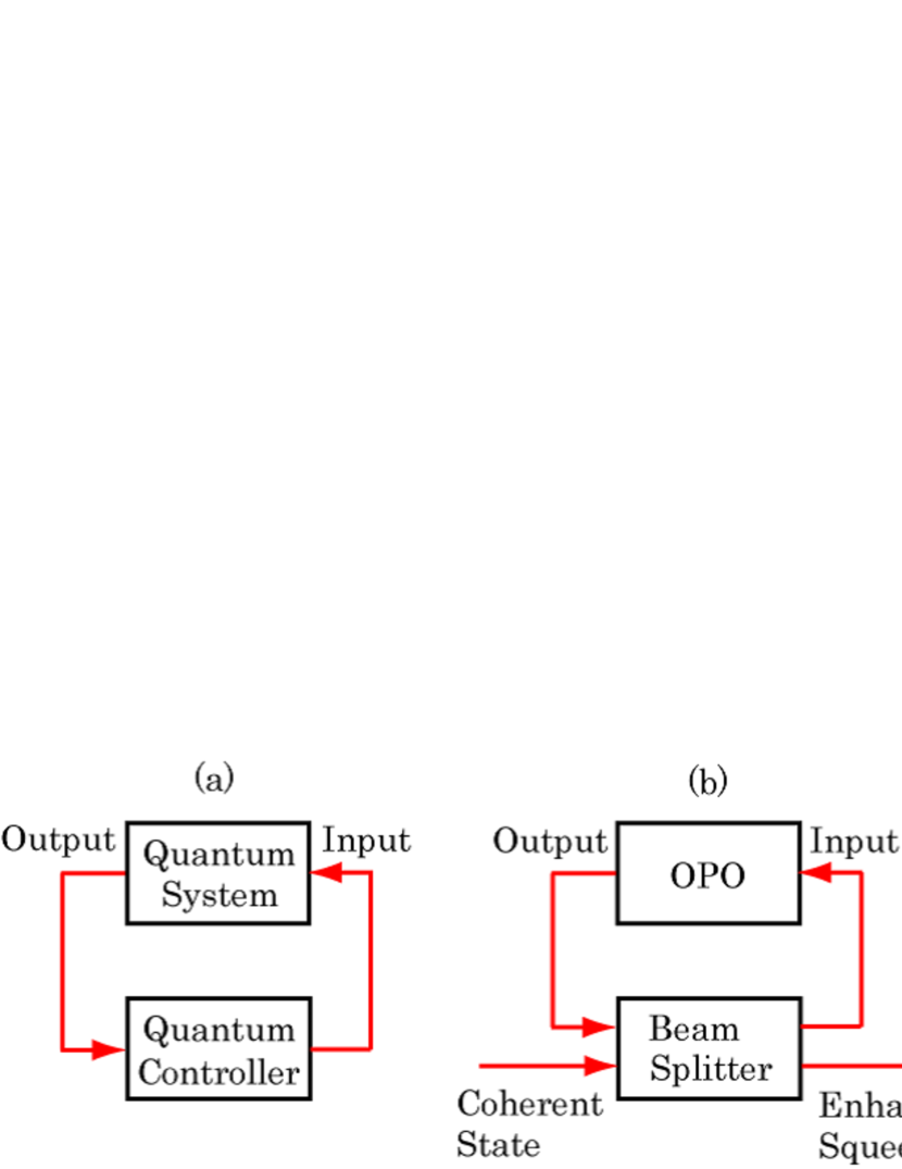
Figure 1: (a) General structure of the CF control. The arrows correspond to unidirectional flows of “quantum signals” such as optical laser fields. (b) Optical system structure of the CF control for squeezing enhancement, corresponding to Fig. 3.

Here we mention about a squeezed state [25]; this is a purely non-classical state where the fundamental quantum noise is reduced below the quantum noise limit in one of the quadrature observables such as the position $\hat{q}$ and the momentum $\hat{p}$ (a more detailed description will be given in Section II). Therefore, a situation in which noise reduction via the CF control shows the best efficiency may appear in problems of generating squeezed states. Actually Yanagisawa [29] and Gough [11] theoretically showed that this idea works in the case of quantum optics. Fig. 1 (b) illustrates the CF loop structure they studied. The quantum system, which now corresponds to an optical parametric oscillator (OPO), has an ability of noise reduction; that is, it transforms an input coherent state into an output squeezed state. It was then shown that the performance of squeezing can be enhanced by constructing an appropriate CF controller, which in this case is given by a beam splitter with tunable transmissivity.

The purpose of this paper is to report the first experimental demonstration of the above-mentioned CF control on optical field squeezing, which well agrees with the theory that carefully takes into account the effects of the actual laboratory setup, particularly time delays and losses in the feedback loop. The results are significant in the sense that, both theoretically and experimentally, they clarify the situation where the CF control is really effective and the limitation on how much it can improve the system performance practically. Note that in [11, 29] a realistic closed loop model was not considered, hence such benefit and limitation are first clarified in this paper. Another important remark is that, while Mabuchi has experimentally demonstrated classical noise reduction with the CF control [20], in our case we deal with purely non-classical noise reduction that beats the quantum noise limit, which is crucial in quantum information processing. In this sense, this paper provides the first experimental demonstration of realistic applicability of the CF control to non-classical regime.

II Preliminaries

In this section we provide some notions of quantum mechanics and the dynamics of an OPO. For more details see [2, 7, 8, 9, 10, 16].

II-A Observables, states, and statistics in quantum optics

In quantum mechanics, unlike the classical case, physical quantities must take different values probabilistically when measuring them. The corresponding statistics is described in terms of a state, which is represented by a unit vector $|{\psi}\rangle$. In general, when measuring a physical quantity represented by a self-adjoint operator $\hat{X}=\hat{X}^{\dagger}$, the mean and variance of the measurement results are respectively given by

$$\langle{\hat{X}}\rangle:=\langle{\psi}|\hat{X}|{\psi}\rangle,~{}~{}~{}\langle{\Delta\hat{X}^{2}}\rangle:=\langle{\psi}|\hat{X}^{2}|{\psi}\rangle-\langle{\psi}|\hat{X}|{\psi}\rangle^{2},$$

where $\langle{\psi}|$ is the adjoint to $|{\psi}\rangle$. That is, a state corresponds to a probability distribution. For these statistical values to take real numbers, $\hat{X}$ must be self-adjoint; actually in quantum mechanics any physical quantity is represented by a self-adjoint operator and is called an observable.

A single-mode quantum optical field is described with an operator $\hat{a}$ and its adjoint $\hat{a}^{\dagger}$, which respectively correspond to a complex amplitude and its conjugate of a classical optical field. These operators satisfy the canonical commutation relation (CCR) $[\hat{a},\hat{a}^{\dagger}]=\hat{a}\hat{a}^{\dagger}-\hat{a}^{\dagger}\hat{a}=1$. These field operators are not self-adjoint, i.e., not observables, hence let us define

$$\hat{x}_{+}:=\hat{a}+\hat{a}^{\dagger},~{}~{}~{}\hat{x}_{-}:=-i(\hat{a}-\hat{a}^{\dagger}).$$

Analogous to the classical case, these observables are called the amplitude and phase quadratures. The CCR for these observables is $[\hat{x}_{+},\hat{x}_{-}]=2i$; due to this equality, for any state the variances satisfy the Heisenberg’s uncertainty relation:

$$\langle{\Delta\hat{x}_{+}^{2}}\rangle\langle{\Delta\hat{x}_{-}^{2}}\rangle\geq 1.$$ (1)

This means that the amplitude and phase quadratures cannot be determined simultaneously. In other words, there is fundamental uncertainty with respect to these two non-commutative observables. In particular, it is known that, for any classical state such as a thermal state, each variance must be bigger than $1$, i.e., $\langle{\Delta\hat{x}_{+}^{2}}\rangle\geq 1$ and $\langle{\Delta\hat{x}_{-}^{2}}\rangle\geq 1$; this lower bound is called the quantum noise limit (QNL). Related to this limit, we here introduce two important states in quantum optics: coherent and squeezed states. A coherent state is the closest possible analogue to a classical electromagnetic wave, which is generated with a laser device. The coherent state $|{\alpha}\rangle$ is defined as an eigenvector of ${\hat{a}}$ with $\alpha\in{\bf C}$ the corresponding eigenvalue, i.e., ${\hat{a}}|{\alpha}\rangle=\alpha|{\alpha}\rangle$. Note that $|{0}\rangle$ represents a vacuum state. A crucial property of $|{\alpha}\rangle$ is that it achieves the QNL, i.e., we have $\langle{\Delta\hat{x}_{+}^{2}}\rangle=\langle{\Delta\hat{x}_{-}^{2}}\rangle=1$ for any $\alpha$, meaning that a coherent state is a lowest-noise classical state. On the other hand, a squeezed state is a purely non-classical state with one of the quadrature variance below the QNL. In particular, for an ideal pure squeezed state the quadrature variances are given by $\langle{\Delta\hat{x}_{+}^{2}}\rangle=e^{2r}$ and $\langle{\Delta\hat{x}_{-}^{2}}\rangle=e^{-2r}$ with $r\in{\bf R}$ a unit-less parameter. Squeezed states play important roles in quantum information technologies, because for instance entanglement, which is a key property to perform various quantum information processing, can be generated using squeezed states. Quantum information processing often relies on highly entangled states, and this equivalently means highly squeezed states are desirable. This is the reason why squeezing enhancement is of vital important.

II-B Optical parametric oscillator as a linear system

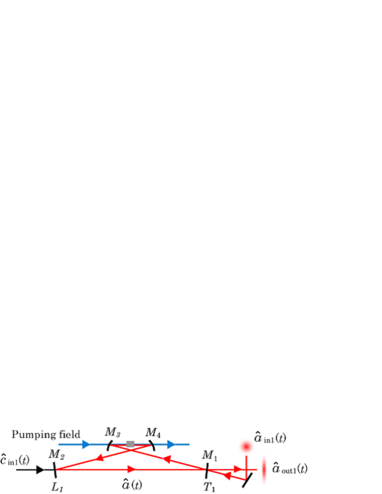
Figure 2: Schematic of the OPO. Arrows represent optical beams travelling along those directions. $M_{i}$ are mirrors $(i=1,\cdots,4)$. A crystal between the curved mirrors $M_{3}$ and $M_{4}$ is a second-order nonlinear medium.

The optical parametric process is a widely-used method for generating a squeezed optical field, where a coherent optical field is squeezed by the interaction with a strong pumping field through a nonlinear medium. To produce a squeezed state of light more effectively, it is common to use the optical parametric oscillator (OPO); a cavity that contains a second-order nonlinear crystal. Fig. 2 shows a conventional bow-tie type cavity with four mirrors, where the mirror $M_{1}$ (input-output port) is partially transmissive and the others are highly reflective for the fundamental optical field. All the mirrors are perfectly transparent for the pumping field. This system renders the input coherent field $\hat{a}_{{\rm in}1}(t)$ interact with the medium many times inside the cavity and finally produces a well-squeezed field $\hat{a}_{{\rm out}1}(t)$ at the output port. These input and output fields couple to the internal cavity field $\hat{a}(t)$ through the mirror $M_{1}$ characterized by the power transmissivity $T_{1}$. Losses inside the OPO are modeled as a coupling between $\hat{a}(t)$ and an unwanted vacuum field $\hat{c}_{{\rm in}1}(t)$ through one of the end mirror $M_{2}$ with the transmissivity $L_{1}$. Here we assume that such interactions occur instantaneously, implying that the outer fields satisfy the CCR $[\hat{a}_{{\rm in}1}(t),\hat{a}^{\dagger}_{{\rm in}1}(t^{\prime})]=\delta(t-t^{\prime})$ and $[\hat{c}_{{\rm in}1}(t),\hat{c}^{\dagger}_{{\rm in}1}(t^{\prime})]=\delta(t-t^{\prime})$.

Let us describe the dynamics of the cavity field $\hat{a}(t)$, which is on resonant with the outer fields. In quantum mechanics, any observable ${\hat{X}}$ changes in time according to the Heisenberg equation $d{\hat{X}}/dt=i[{\hat{X}},{\hat{H}}]$, where $\hat{H}=\hat{H}^{\dagger}$ is called the Hamiltonian. Now the Hamiltonian only for $\hat{a}(t)$ is given by

$$\hat{H}=\omega_{0}\hat{a}^{\dagger}(t)\hat{a}(t)+\frac{i}{2}\big{[}\epsilon e^{-i2\omega_{0}t}\hat{a}^{\dagger}(t)\mbox{}^{2}-\epsilon^{\ast}e^{i2\omega_{0}t}\hat{a}(t)^{2}\big{]},$$

where $\omega_{0}$ is the resonant frequency and $\epsilon$ denotes the effectiveness of the nonlinear medium which depends on the pumping field strength of frequency $2\omega_{0}$. The Heisenberg equation of $\hat{a}(t)$ that involves the coupling to the outer fields is given by the following quantum Langevin equation [2, 7, 9, 10]:

$$\frac{d\hat{a}(t)}{dt}=-i\omega_{0}\hat{a}(t)+\epsilon e^{-2i\omega_{0}t}\hat{a}^{\dagger}(t)-\frac{\gamma}{2}\hat{a}(t)$$

$$\hskip 50.00008pt\mbox{}+\sqrt{\gamma_{1}}\hat{a}_{{\rm in}1}(t)+\sqrt{\gamma_{L1}}\hat{c}_{{\rm in}1}(t),$$ (2)

where $\gamma:=\gamma_{1}+\gamma_{L1}$, and $\gamma_{1}:=cT_{1}/l$ and $\gamma_{L1}:=cL_{1}/l$ represent the damping rates with $l$ the optical path length in the OPO and $c$ the speed of light. The outer fields satisfy the following boundary condition:

$$\hat{a}_{{\rm out}1}(t)=\sqrt{\gamma_{1}}\hat{a}(t)-\hat{a}_{{\rm in}1}(t).$$ (3)

The single-input and single-output linear system given by Eqs. (II-B) and (3) is the system generating a squeezed state of light.

As in the classical case, a simple input-output relation is found in the Fourier domain $\hat{O}(\Omega)=\int dt\hat{O}(t)e^{i\Omega t}/\sqrt{2\pi}$, where we have moved to the rotating frame at frequency $\omega_{0}$ by setting $\hat{O}(t)=\hat{o}(t)e^{i\omega_{0}t}$. We will deal with for instance $\hat{A}_{{\rm in}1}(\Omega)$ and $\hat{A}^{\dagger}_{{\rm out}1}(\Omega)$, that corresponds to $\hat{a}_{{\rm in}1}(t)$ and $\hat{a}^{\dagger}_{{\rm out}1}(t)$, respectively. As a result we have

$$\hat{A}_{{\rm out}1}(\Omega)=G(\Omega)\hat{A}_{{\rm in}1}(\Omega)+g(\Omega)\hat{A}_{{\rm in}1}^{\dagger}(\Omega)$$

$$\hskip 50.00008pt\mbox{}+\bar{G}(\Omega)\hat{C}_{{\rm in}1}(\Omega)+\bar{g}(\Omega)\hat{C}_{{\rm in}1}^{\dagger}(\Omega),$$ (4)

where

$$G(\Omega)= \frac{(\gamma_{1}/2)^{2}-(\gamma_{L1}/2-i\Omega)^{2}+|\epsilon|^{2}}{(\gamma/2-i\Omega)^{2}-|\epsilon|^{2}},~{}~{}$$

$$\bar{G}(\Omega)= \frac{\sqrt{\gamma_{1}\gamma_{L1}}(\gamma/2-i\Omega)}{(\gamma/2-i\Omega)^{2}-|\epsilon|^{2}},~{}~{}g(\Omega)=\frac{\epsilon\gamma_{1}}{(\gamma/2-i\Omega)^{2}-|\epsilon|^{2}},$$

and $\bar{g}(\Omega)=\sqrt{\gamma_{L1}/\gamma_{1}}g(\Omega)$. To evaluate the squeezing, let us introduce the (generalized) quadrature in the Fourier domain:

$$\hat{X}^{\theta}_{{\rm out}1}(\Omega)=\frac{1}{2}\big{[}e^{i\theta}\hat{A}_{{\rm out}1}(\Omega)+e^{-i\theta}\hat{A}_{{\rm out}1}^{\dagger}(\Omega)\big{]}.$$ (5)

We write $\hat{X}^{+}_{{\rm out}1}(\Omega)=\hat{X}^{0}_{{\rm out}1}(\Omega)$ and $\hat{X}^{-}_{{\rm out}1}(\Omega)=\hat{X}^{\pi/2}_{{\rm out}1}(\Omega)$. For $\hat{A}_{{\rm in}1}(\Omega)$ and $\hat{C}_{{\rm in}1}(\Omega)$ their quadratures are defined in the same form as Eq. (5). Then, from Eq. (II-B) we have

$$\hat{X}_{{\rm out}1}^{\pm}(\Omega)=[G(\Omega)\pm g(\Omega)]\hat{X}^{\pm}_{{\rm in}1}(\Omega)+[\bar{G}(\Omega)\pm\bar{g}(\Omega)]\hat{X}^{\pm}_{L1}(\Omega).$$

The variance of $\hat{X}_{{\rm out}1}^{\pm}(\Omega)$ is simply given by the power spectrum $S^{\pm}_{{\rm out}1}(\Omega):=\langle|\hat{X}^{\pm}_{{\rm out}1}(\Omega)|^{2}\rangle$. In particular, when the input field is a vacuum state, we have

$$S^{\pm}_{{\rm out}1}(\Omega)=|G(\Omega)\pm g(\Omega)|^{2}+|\bar{G}(\Omega)\pm\bar{g}(\Omega)|^{2}.$$

If $\epsilon=0$, then $S^{\pm}_{{\rm out}1}(\Omega)=1,~{}\forall\Omega$, which is the QNL. But a squeezed state of light is generated when $\epsilon\neq 0$; actually for simplicity in the case $\gamma_{L1}=0,\epsilon\in{\bf R}$, and $\Omega=0$, we have

$$S^{+}_{{\rm out}1}(0)=\Big{(}\frac{\gamma_{1}+2\epsilon}{\gamma_{1}-2\epsilon}\Big{)}^{2},~{}~{}~{}S^{-}_{{\rm out}1}(0)=\Big{(}\frac{\gamma_{1}-2\epsilon}{\gamma_{1}+2\epsilon}\Big{)}^{2},$$

one of which is below the QNL. Note that the sign of $\epsilon$ determines which quadrature is squeezed or anti-squeezed.

III Coherent feedback control on optical field squeezing

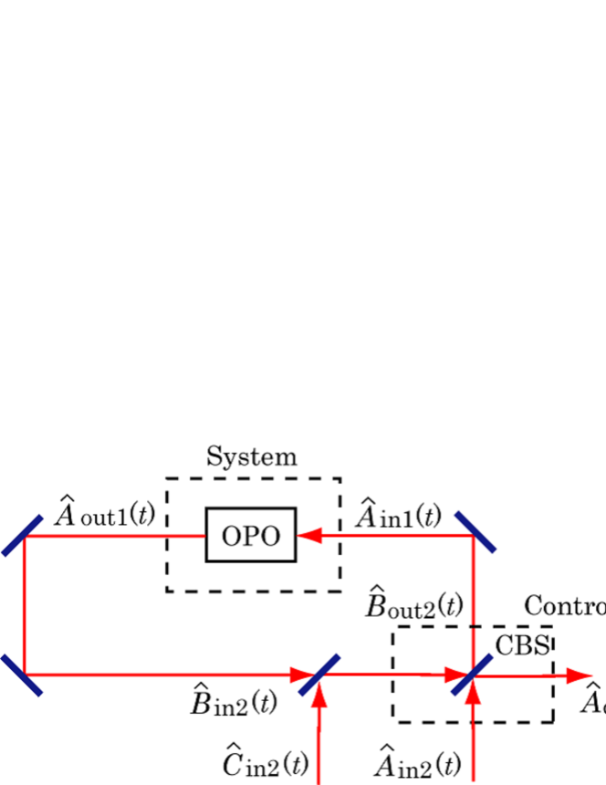
Figure 3: Schematic of the CF control on optical field squeezing.

The basic idea of the CF control for optical squeezing enhancement is found in [11, 29]. We here study a realistic model corresponding to an actually constructed optical system in the laboratory, which takes into account time delays and losses in the feedback loop.

The CF structure is depicted in Fig. 3. The system is the OPO described in Sec. II. B. In this CF control scheme, a beam splitter (BS) plays the roles of both a controller and an input-output port. Hereafter we name this BS as the control-BS (CBS) to discern it from the other BSs. The transmissivity $T_{2}$ of the CBS is tuned to obtain higher squeezing level. The coherent input field $\hat{A}_{{\rm in}2}(t)$ is sent to one port of the CBS, and then, one of its outputs $\hat{B}_{{\rm out}2}(t)$ is sent to the OPO. The output of the OPO, $\hat{A}_{{\rm out}1}(t)$, is sent back to the CBS to close the loop. Finally at the other output port of the CBS we will find an enhanced squeezed field $\hat{A}_{{\rm out}2}(t)$. The input-output relation at the CBS is given by (in the rotating frame)

$$\hat{A}_{{\rm out}2}(t)= \sqrt{1-T_{2}}\hat{A}_{{\rm in}2}(t)$$

$$+\sqrt{T_{2}}\big{[}\sqrt{1-L_{2}}\hat{B}_{{\rm in}2}(t)+\sqrt{L_{2}}\hat{C}_{{\rm in}2}(t)\big{]},$$

$$\hat{B}_{{\rm out}2}(t)= -\sqrt{1-T_{2}}\big{[}\sqrt{1-L_{2}}\hat{B}_{{\rm in}2}(t)+\sqrt{L_{2}}\hat{C}_{{\rm in}2}(t)\big{]}$$

$$+\sqrt{T_{2}}\hat{A}_{{\rm in}2}(t),$$

where $\hat{C}_{{\rm in}2}(t)$ is a vacuum field entering through a fictitious BS with reflectivity $L_{2}$, and this is a model of losses in the CF loop. $\hat{B}_{{\rm in}2}(t)$ is the output of the OPO just before entering this fictitious BS. Here it is assumed that the fictitious BS is placed just before the CBS. Now let $\tau_{a}:={l_{a}}/{c}$ ($\tau_{b}:={l_{b}}/{c}$) be the time delay resulting from the optical path length $l_{a}$ ($l_{b}$) from (to) the CBS to (from) the OPO. Then we have

$$\hat{A}_{{\rm in}1}(t)=\hat{B}_{{\rm out}2}(t-\tau_{a})e^{i\omega_{0}\tau_{a}},~{}~{}\hat{B}_{{\rm in}2}(t)=\hat{A}_{{\rm out}1}(t-\tau_{b})e^{i\omega_{0}\tau_{b}}.$$

Combining these equations with Eq. (II-B) the final input-output relation is given in terms of the quadrature representation by

$$\hat{X}^{\pm}_{{\rm out}2}(\Omega)$$

$$\mbox{}=\Big{[}\sqrt{1-T_{2}}+\frac{T_{2}\sqrt{1-L_{2}}\alpha^{\pm}(\Omega)}{1+\alpha^{\pm}(\Omega)\sqrt{(1-T_{2})(1-L_{2})}}\Big{]}\hat{X}^{\pm}_{{\rm in}2}(\Omega)$$

$$\mbox{}+\frac{\sqrt{T_{2}(1-L_{2})}\beta^{\pm}(\Omega)}{1+\alpha^{\pm}(\Omega)\sqrt{(1-T_{2})(1-L_{2})}}\hat{X}^{\pm}_{L1}(\Omega)$$

$$\mbox{}+\Big{[}\sqrt{T_{2}L_{2}}-\frac{\sqrt{T_{2}(1-L_{2})(1-T_{2})L_{2}}\alpha^{\pm}(\Omega)}{1+\alpha^{\pm}(\Omega)\sqrt{(1-T_{2})(1-L_{2})}}\Big{]}\hat{X}^{\pm}_{L2}(\Omega),$$

where $\alpha^{\pm}(\Omega)=[G(\Omega)\pm g(\Omega)]e^{i(\Omega+\omega_{0})(\tau_{a}+\tau_{b})}$ and $\beta^{\pm}(\Omega)=[\bar{G}(\Omega)\pm\bar{g}(\Omega)]e^{i(\Omega+\omega_{0})\tau_{b}}$. When the input is a vacuum state, the power spectrum $S^{\pm}_{{\rm out}2}(\Omega):=\langle|\hat{X}^{\pm}_{{\rm out}2}(\Omega)|^{2}\rangle$ is given by

$$S^{\pm}_{{\rm out}2}(\Omega)=\Big{|}\sqrt{1-T_{2}}+\frac{T_{2}\sqrt{1-L_{2}}\alpha^{\pm}(\Omega)}{1+\alpha^{\pm}(\Omega)\sqrt{(1-T_{2})(1-L_{2})}}\Big{|}^{2}$$

$$\hskip 25.00003pt\mbox{}+\frac{T_{2}(1-L_{2})|\beta^{\pm}(\Omega)|^{2}}{|1+\alpha^{\pm}(\Omega)\sqrt{(1-T_{2})(1-L_{2})}|^{2}}$$

$$\hskip 25.00003pt\mbox{}+\Big{|}\sqrt{T_{2}L_{2}}-\frac{\sqrt{T_{2}(1-L_{2})(1-T_{2})L_{2}}\alpha^{\pm}(\Omega)}{1+\alpha^{\pm}(\Omega)\sqrt{(1-T_{2})(1-L_{2})}}\Big{|}^{2}.$$

It is immediately verified $S^{\pm}_{{\rm out}1}(\Omega)=S^{\pm}_{{\rm out}2}(\Omega)$ when the system is just the uncontrolled OPO described in Section II-B, i.e., $T_{2}=1$ and $L_{2}=0$. Also $L_{2}=1$ leads to $S^{\pm}_{{\rm out}2}(\Omega)=1~{}\forall\Omega$, implying that the CF loop loss will cause the overall degradation of squeezing level in frequency. The time delays appearing in $\alpha^{\pm}(\Omega)$ will affect on the control performance as well, particularly for the effective bandwidth in frequency. This will be seen later on. In what follows we assume that the CF loop is on resonance, i.e., $e^{i\omega_{0}(\tau_{a}+\tau_{b})}=-1$.

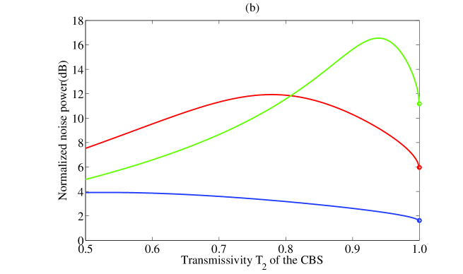
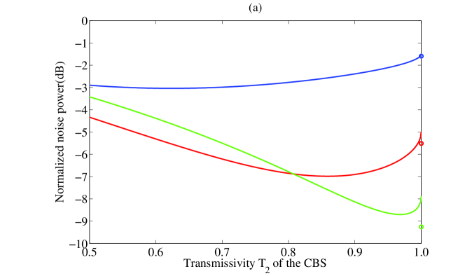
Figure 4: The transmissivity $T_{2}$ of the CBS versus the (a) anti-squeezing and (b) squeezing levels for various normalized pumping strength $x$. The blue, red, and green lines correspond to $x=0.1$, $x=0.35$, and $x=0.6$, respectively. The circles indicate the values at $T_{2}=1$ with $L_{2}=0$, corresponding to the uncontrolled OPO.

Let us numerically evaluate the performance of how much the CF control can enhance the squeezing, or equivalently, can reduce the noise further. Here a set of practical values of parameters are taken [24]: $T_{1}=0.12$, $L_{1}=5.0\times 10^{-3}$, $L_{2}=5.0\times 10^{-2}$, $l=0.5$ m, and $l_{a}=l_{b}=0.25$ m. To calculate $S^{\pm}_{{\rm out}2}(\Omega)$ we particularly focus on the values at frequency $\Omega/2\pi=1$ MHz. Fig. 4 depicts how the (a) anti-squeezing and (b) squeezing levels depend on $T_{2}$, with various values of the normalized pumping strength $x:=2|\epsilon|/\gamma$. Here, the power spectrum is shown in the unit of normalized magnitude, i.e., $10\log_{10}(S^{\pm}_{{\rm out}2}/S^{\pm}_{{\rm in}2})$ dB, where $S^{\pm}_{{\rm in}2}(\Omega):=\langle|\hat{X}^{\pm}_{{\rm in}2}(\Omega)|^{2}\rangle=1$ is the power of the vacuum input. Thus the horizontal axis ($0$ dB) corresponds to the QNL. Now the circles indicate the values at $T_{2}=1$ with $L_{2}=0$, i.e., the squeezing and anti-squeezing levels of the uncontrolled OPO. Then, in the case of weak pumping ($x=0.1$ or $x=0.35$), we find $T_{2}$ such that the squeezing level is enhanced by the CF control compared to that of the uncontrolled OPO. However, in the case of strong pumping ($x=0.6$), the CF control cannot enhance the squeezing at all. This is understood by considering the trade-off between the enhancement of the nonlinear squeezing effect and the CF loop loss; that is, the more strongly the CF control enhances the nonlinear effect, the more loss it must incur. Therefore, when the OPO is already pumped strongly, the CF loop loss becomes dominant compared to the enhancement of the nonlinear effect, and we cannot perform much enhancement of the squeezing. This is a limitation of the CF control for the squeezing enhancing problem.

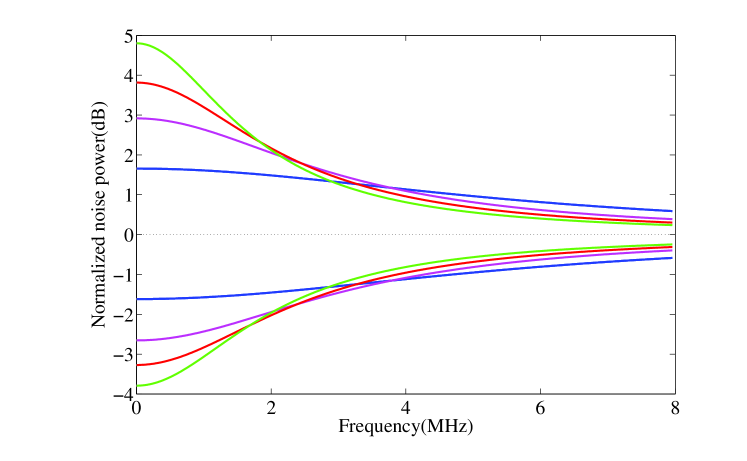
Figure 5: Frequency dependences of the squeezing and anti-squeezing levels. The green, red, pink, and blue lines represent those under the condition of $T_{2}$=0.7, 0.8, 0.9, and 1.0, respectively.

Next, to see the frequency-dependence of the CF control, we calculate $S^{\pm}_{{\rm out}2}(\Omega)$ with fixed value at $x=0.1$, which in the above discussion was proven to be a value such that the CF control has clear benefit. Fig. 5 shows the squeezing and anti-squeezing levels in the following cases: $T_{2}$=0.7, 0.8, 0.9, and 1.0. Now the squeezing and anti-squeezing levels of the uncontrolled OPO are almost the same as those with $T_{2}=1$ and $L_{2}=0.05$, which are indicated by the blue lines. Therefore, the squeezing enhancement can be evaluated by simply comparing the squeezing level with the CF ($T_{2}\neq 1$) to that without the CF ($T_{2}=1$), for a fixed value of $L_{2}$. (Note this argument makes sense only in the case of weak pumping power.) Then, in each case of $T_{2}$, the squeezing enhancement is observed only at lower frequencies. Moreover, while better squeezing is achieved by taking a smaller value of $T_{2}$, this brings the narrower effective bandwidth in frequency. This additional limiting property of the CF control is mainly due to the time delays occurred in the OPO and the feedback loop.

IV The coherent feedback experiment

IV-A Experimental setup

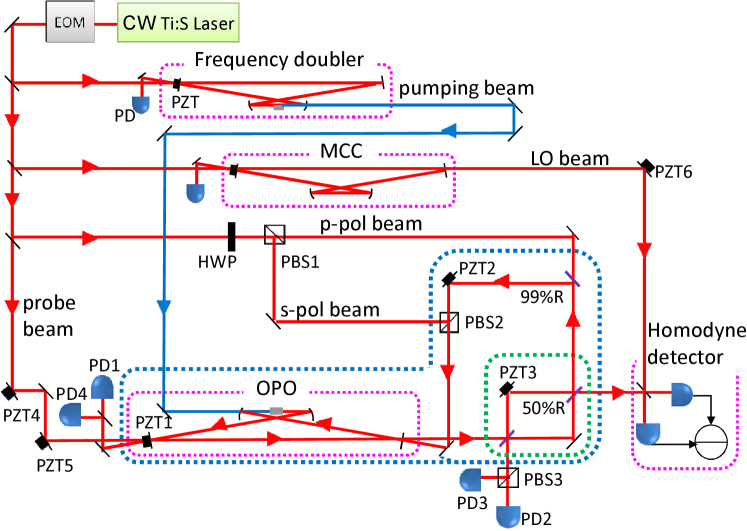
Figure 6: Experimental configuration. OPO: optical parametric oscillator, MCC: mode cleaning cavity, PD: photo detector, PZT: piezoelectric transducer, PBS: polarized beam splitter, HWP: half wave plate, and LO: local oscillator. The blue dashed line indicates the CF loop. The green dashed line indicates the Mach-Zehnder interferometer, which corresponds to the CBS.

Fig. 6 shows our experimental setup. The light source is a continuous-wave Ti:Sapphire laser (Coherent, MBR-110). The wavelength is 860 nm and the beam is horizontally polarized. A phase modulation of 10.4 MHz is applied on the beam for locking of all cavities by Pound-Drever-Hall method [4, 6].

The system is composed of four parts. The first is a frequency-doubler, which is a cavity to generate a second harmonic beam of 430 nm [22]. This beam is used as a pumping beam for the OPO. The second is a mode-cleaning cavity that is used to clean up the spatial mode of local oscillator (LO) for homodyne detection so as to attain higher mode matching between the LO and the squeezed beam.

The third part consists of the OPO, the CBS, and the CF loop. The structure of the OPO is the same as in [24]. In order to realize several locking, a probe beam is injected into the OPO from the high-reflection-coated mirror. The reflected beam is detected with PD1 and PD4 to get error signals for locking the cavity and the relative phase between the probe beam and the pumping beam. To lock the cavity we demodulate the output of the PD1 with 10.4 MHz modulation signal, and feed back the error signal to PZT1. On the other hand, to lock the relative phase between the probe beam and the pumping beam, we apply a phase modulation of 107 kHz on the probe beam with PZT4. We demodulate the output of the PD4 with 107 kHz modulation signal, and feed back the error signal to PZT5. Furthermore, we obtain the probe beam at the output port of the OPO which is used to lock the relative phase between the probe and the LO beams as explained later.

The CBS is realized by using a Mach-Zehnder (MZ) interferometer. The transmissivity can be determined by adjusting the phase difference between two arms in the MZ interferometer. In order to lock a particular transmissivity, a s-polarized (s-pol) beam is injected into the CF loop from PBS2. Note that this s-pol beam does not circulate in the CF loop. The beam is detected by PD3 to give the error signal of the CBS, which is fed back to PZT3. Additionally, to lock the CF loop, we inject a p-polarized (p-pol) beam into the CF loop from the mirror of 0.99 reflectivity. Note that this beam and the squeezed beam counter-propagate, hence this beam does not contaminate the CF output (the squeezed beam). We obtain the error signal by demodulating the output of PD2 with 10.7 MHz modulation signal, and feed back it to PZT2.

The last part is homodyne detection. In order to measure a specific quadrature amplitude accurately, the relative phase between the probe beam (equivalently, the squeezed beam) and the LO beam should be locked. The error signal is obtained from the output of the homodyne detector by demodulating it with 107 kHz modulation signal. The error signal is fed back to PZT6. When measuring the squeezed beam, the probe beam is set to 4 $\mu$W, and the LO beam is set to 3 mW, so that we can attain high signal-to-noise ratio without saturation of the homodyne detector. The output of the homodyne detector is measured with a spectrum analyzer.

IV-B Results and discussion

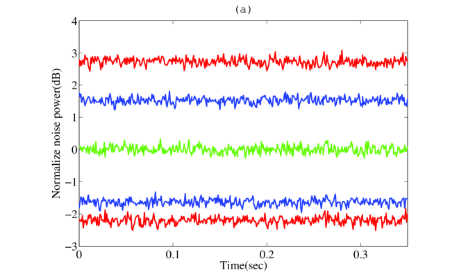
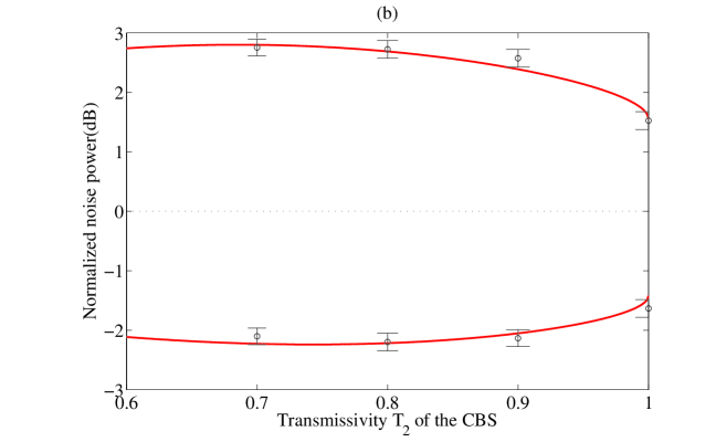
Figure 7: (a) Measurement results of the squeezing and anti-squeezing levels at center frequency of 2.5 MHz. The green line represents the vacuum noise level, i.e., the QNL. The blue lines represent the squeezing and anti-squeezing levels without the CF, and the red lines represent those with the CF when $T_{2}=0.8$. All the traces are averaged over 50 times. Dark noise is subtracted. (b) $T_{2}$-dependence of the squeezing and anti-squeezing levels at center frequency of 2.5 MHz. Circles and solid curves represent experimental and theoretical values, respectively.

The parameters in this experiment are: $x=0.111$, $T_{1}=0.20$, $L_{1}=6.5\times 10^{-3}$, $L_{2}=0.12$, $l=0.5$ m, and $l_{a}=l_{b}=0.25$ m. First we measure the squeezing and anti-squeezing levels with the CF ($T_{2}=0.8$) and those without the CF ($T_{2}=1.0)$. Note again that the squeezing enhancement can be evaluated by comparing these two values. Fig. 7 (a) shows the measurement results. The center frequency, the resolution bandwidth, and the video bandwidth is $\Omega/2\pi=2.5$ MHz, 30 kHz, and 300 Hz, respectively. Here, because of a practical reason explained later, we cannot take the frequency $\Omega/2\pi=1$ MHz unlike the case discussed in Section III. The green line represents the vacuum noise level, i.e., the QNL. The blue lines represent the squeezing and anti-squeezing levels without the CF, and the red lines represent those with the CF. All the traces are normalized to the QNL. Fig. 7 (a) clearly demonstrates the effect of the CF, showing the squeezing enhancement from $-$1.64$\pm$0.15 dB to $-$2.20$\pm$0.15 dB and the anti-squeezing enhancement from 1.52$\pm$0.15 dB to 2.72$\pm$0.15 dB.

We carry out measurements with several $T_{2}$; Fig. 7 (b) shows $T_{2}$-dependence of the squeezing and anti-squeezing levels. Circles stand for the measurement results, and solid lines show the following theoretical values [24]: $S^{\prime\prime}_{\pm}(\Omega)=1+\eta(S^{\pm}_{{\rm out}2}(\Omega)-1)$, where $\eta$ represents the overall detection efficiency given by $\eta=\xi^{2}\rho$, $\xi$ is homodyne visibility and $\rho$ is quantum efficiency of photo diodes in the homodyne detector. In our experiment, we obtain $\eta=0.961$ with $\xi=0.985$, and $\rho=0.99$. Experimental and theoretical values show good agreement. Marginal gaps are attributed to fluctuation of the phase and the MZ interferometer locking.

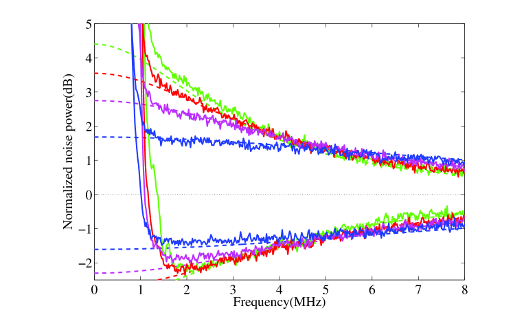
Figure 8: Frequency dependence of the squeezing and anti-squeezing levels. The blue lines represent those without the CF, while the green, red, and pink lines correspond to the case with the CF under the condition of $T_{2}$=0.7, 0.8, and 0.9, respectively. Dark noise is subtracted. Dashed lines indicate theoretical values.

A feature of the CF control can be seen in broadband measurement, where in this experiment we have observed that $x$ and $L_{1}$ are a bit changed to: $x=0.106$ and $L_{1}=9.0\times 10^{-3}$. Fig. 8 shows the frequency-dependence of the squeezing and anti-squeezing levels up to 8 MHz. The blue solid lines represent those without the CF, while the green, red, and pink solid lines correspond to the case with the CF under the condition of $T_{2}$=0.7, 0.8, and 0.9, respectively. At lower frequencies we find large laser noises and modulation signals used for several locking. This is the reason why, in our experiment, highly effective squeezing enhancement at for instance $\Omega/2\pi=1$ MHz cannot be observed; hence this is a practical limitation of the CF control. Except along such a noisy region in frequency, the results show good agreements with theoretical values illustrated with dashed lines, which are almost the same as those shown in Fig. 5. That is, as discussed in Section III, better squeezing enhancement certainly brings the narrower effective bandwidth in frequency.

V Conclusion

The first experimental demonstration of the CF control for squeezing enhancement is demonstrated. The results well agree with the theory that carefully takes into account the effects of the actual laboratory setup particularly time delays and losses occurring in the feedback loop. Although our feedback system is limited to linear optics, the results obtained in this work suggest realistic applicability of the CF control to various highly nonlinear quantum systems such as nanophotonic circuits [15, 21], which can be used for quantum error correction.

References

- [1] C. Ahn, A. C. Doherty, and A. J. Landahl, Continuous quantum error correction via quantum feedback control, Phys. Rev. A, vol. 65, p. 042301, 2002.
- [2] H. A. Bachor and T. C. Ralph, A guide to experiments in quantum optics, John Wiley, 2004.
- [3] V. P. Belavkin, Quantum stochastic calculus and quantum nonlinear filtering, J. Multivariate Anal., vol. 42, pp. 171-201, 1992.
- [4] E. D. Black, An introduction to Pound–Drever–Hall laser frequency stabilization, Am. J. Phys., vol. 69, p. 79, 2001.
- [5] L. Bouten, R. van Handel, and M. R. James, An introduction to quantum filtering, SIAM J. Contr. Optim., vol. 46-6, pp. 2199-2241, 2007.
- [6] R. A. Boyd, J. L. Bliss, and K. G. Libbrecht, Teaching physics with 670-nm diode lasers-experiments with Fabry-Perot cavities, Am. J. Phys., vol. 64, pp. 1109-1115, 1996.
- [7] M. J. Collet and C. W. Gardiner, Squeezing of intracavity and traveling-wave light fields produced in parametric amplification, Phys. Rev. A, vol. 30, p. 1386, 1984.
- [8] A. Furusawa and P. van Loock, Quantum Teleportation and Entanglement: A Hybrid Approach to Optical Quantum Information Processing, Wiley-VCH, Berlin, 2011.
- [9] C. W. Gardiner and M. J. Collet, Input and Output in damped quantum systems, Phys. Rev. A, vol. 31, p. 3761, 1984.
- [10] C. W. Gardiner and P. Zoller, Quantum Noise, Springer Berlin, 2004.
- [11] J. E. Gough and S. Wildfeuer, Enhancement of field squeezing using coherent feedback, Phys. Rev. A, vol. 80, p. 42107, 2009.
- [12] J. E. Gough and M. R. James, The series product and its application to quantum feedforward and feedback networks, IEEE Trans. Automatic Contr., vol. 54-11, pp. 2530-2544, 2009.
- [13] J. E. Gough, M. R. James, and H. I. Nurdin, Squeezing components in linear quantum feedback networks, Phys. Rev. A, vol. 81, p. 023804, 2010.
- [14] M. R. James, H. I. Nurdin, and I. R. Petersen, control of linear quantum stochastic systems, IEEE Trans. Automat. Contr., vol. 53-8, pp. 1787-1803, 2008.
- [15] J. Kerckhoff, H. I. Nurdin, D. Pavlichin, and H. Mabuchi, Coherent feedback formulation of a continuous quantum error correction protocol, Phys. Rev. Lett., vol. 105, p. 040502, 2010.
- [16] U. Leonhardt, Essential Quantum Optics: From Quantum Measurements to Black Holes, Cambridge Univ. Press, 2010.
- [17] S. Lloyd, Coherent quantum feedback, Phys. Rev. A, vol. 62, p. 022108, 2003.
- [18] A. I. Maalouf and I. R. Petersen, Coherent LQG control for a class of linear complex quantum systems, in Proceedings of ECC, Hungary, 2009.
- [19] A. I. Maalouf and I. R. Petersen, Coherent control for a class of annihilation operator linear quantum systems, IEEE Trans. Automat. Contr., vol. 56-2, pp. 309-319, 2011.
- [20] H. Mabuchi, Coherent-feedback quantum control with a dynamic compensator, Phys. Rev. A, vol. 78, p. 32323, 2008.
- [21] H. Mabuchi, Coherent-feedback control strategy to suppress spontaneous switching in ultra-low power optical bistability, arXiv:1101.3461, 2011.
- [22] G. Masada, T. Suzudo, Y. Satoh, H. Ishizuki, T. Taira, and A. Furusawa, Efficient generation of highly squeezed light with periodically poled MgO:LiNbO3, Opt. Express, vol. 18, p. 13114, 2010.
- [23] H. I. Nurdin, M. R. James, and I. R. Petersen, Coherent quantum LQG control, Automatica, vol. 45, pp. 1837-1846, 2009.
- [24] Y. Takeno, M. Yukawa, H. Yonezawa, and A. Furusawa, Observation of-9 dB quadrature squeezing with improvement of phase stability in homodyne measurement, Opt. Express, vol. 15, p. 4321, 2007.
- [25] D. F. Walls, Squeezed states of light, Nature, vol. 306, pp. 141-146, 1983.
- [26] H. M. Wiseman and G. J. Milburn, All-optical versus electro-optical quantum-limited feedback, Phys. Rev. A, vol. 49, p. 4110, 1994.
- [27] H. W. Wiseman and G. J. Milburn, Quantum Measurement and Control, Cambridge University Press, 2009.
- [28] M. Yanagisawa and H. Kimura, Transfer function approach to quantum control– Part I: Dynamics of quantum feedback systems, IEEE Trans. Automat. Contr., vol. 48-12, pp. 2107-2120, 2003.
- [29] M. Yanagisawa and H. Kimura, Transfer function approach to quantum control– Part II: Control concepts and applications, IEEE Trans. Automat. Contr., vol. 48-12, pp. 2121-2132, 2003.