Chaotic behavior of a class of discontinuous dynamical systems of fractional-order

Abstract

In this paper the chaos persistence in a class of discontinuous dynamical systems of fractional-order is analyzed. To that end, the Initial Value Problem is first transformed, by using the Filippov regularization [1], into a set-valued problem of fractional-order, then by Cellina’s approximate selection theorem [2, 3], the problem is approximated into a single-valued fractional-order problem, which is numerically solved by using a numerical scheme proposed by Diethelm, Ford  and Freed [4]. Two typical examples of systems belonging to this class are analyzed and simulated.

Kkeyword Fractional derivative; discontinuous dynamical system; Filippov regularization; differential inclusion; numerical method

1 Introduction

Dynamical systems (d.s.), discontinuous with respect to the state variable, occur in a large number of problems, especially from mechanics (dry friction with stick and slip modes, impacts, oscillating systems with viscous damping, elasto-plasticity, alternatively forced vibrations, braking processes with locking phases), electrical engineering (electrical circuits and networks with switches, power electronics), automatic and optimal control theory, convex optimizations, game theory, non-smooth control systems synthesis, uncertain systems, walking machines, biological and physiological systems and everywhere non-smooth characteristics are used to represent switches (see e.g. [5, 6, 7, 8, 9, 10] and some references therein). In other words, in the real word non-smoothness is a common phenomenon. The underlying mathematical models are generally described by a set of first-order differential equations with discontinuous components. Particularly, the discontinuity is due to the discontinuity of the state variable, of the associated vector field, of the Jacobian, or to higher-order discontinuity.

In practical examples, the discontinuity appears because of piecewise continuous or switch-like functions (e.g. signum, absolute value, Heaviside function -also known as the “unit step function”- maximum function, etc.).

On the other hand, there are many continuous d.s. which display fractional-order dynamics. These mathematical phenomena allow to describe a real object more accurately than do classical “integer” dynamics. One of the main reasons to use the integer-order models was the absence of methods for fractional differential equations.

The real objects or phenomena such as viscoelastic systems, dielectric polarization, electrochemistry, percolation, material science, polymer modeling, theory of ultra-slow processes, electromagnetic waves, evolution of complex systems, financial processes, secure communication, etc. are generally fractional (see [11, 12, 13, 14, 15, 16, 17, 18, 19]).

We consider in this paper a class of unified Filippov discontinuous d.s. of fractional-order and prove that the underlying Initial Value Problem (I.V.P.) admits solutions which can be numerically determined. We also prove numerically that in these systems of lower than third order chaos may appear (as it is known, in the case of integer order, according to the well known Poincar -Bendixon theorem, chaos appears only at systems of minimum order three).

These systems are modeled by the following autonomous I.V.P.

$$\frac{d^{q}x(t)}{dt^{q}}=g(x(t))+A~{}s(x(t)),~{}x(0)=x_{0},~{}t\in I=[0,\infty),$$ (1)

with$~{}g:\mathbb{R}^{n}\rightarrow\mathbb{R}^{n},~{}A=\left(b_{i,j}\right)_{n\asymp n}$ real constant matrix, the vector function $s:\mathbb{R}^{n}\rightarrow\mathbb{R}^{n}$ being composed of signum functions (the most encountered case), i.e.

$$s(x)=\left(\begin{array}[]{c}sgn(x_{1})\\ \vdots\\ sgn(x_{n})\end{array}\right),$$ (2)

$q$ the fractional order, $0<q\leq 1$ (although there are also some applications for $q>1,~{}$ as is the case in many applications).

The right-hand side depends on $p\in\mathbb{R},\mathbb{~{}}$the control parameter.

Hereafter, we impose the following assumption on the discontinuous right-hand functions

(H1):The right-hand side is piecewise continuous (continuous on a finite number of $m$ open domains $D_{i}\subset R^{n}$,$~{}i=1,2,\ldots,m$, and has finite (possibly different) limits from different boundary points, i.e. bounded discontinuities), $g$ being continuous (linear function in the great majority of practical examples). The null set of the discontinuity (switch) points is $M=R^{n}\backslash\cup D_{i}$.

At every $M$ point, the discontinuity surface is a hyperplane (plane for $n=3).$

The considered class of systems is autonomous. Thus, the I.V.P. (1) can be written as follows

$$\frac{d^{q}x}{dt^{q}}=g(x)+A~{}s(x),~{}x(0)=x_{0},~{}t\in I.$$ (3)

To achieve our goal, we consider the I.V.P. (3) in a more familiar framework, such as differential inclusions and differential equations of fractional-order.

The paper is organized as follows: In Section 2, the discontinuous I.V.P. (3) is transformed, via Filippov’s regularization, into a set-valued I.V.P. and then into a continuous differential equation of fractional-order via Cellina’s Theorem [2, 3]. In Section 3 the numerical integration of differential equations of fractional-order, which will be used to integrate the obtained I.V.P. (3), is presented briefly. In Section 4 this algorithm is used to investigate the lowest-order $q$ for which chaos vanishes in two representative chaotic systems.

2 Continuous approximation of I.V.P. (3)

One of the first questions of set-valued analysis is how to relate set-valued and single-valued functions, so as to avoid dealing with the set-valued functions. Because the considered examples in this paper are modeled by three-dimensional real I.V.P., the next results will be particularized in the Euclidean space $\mathbb{R}^{n},$ some of them are valid even in more general (such as Hilbert) spaces.

First, let us consider the IVP (3) in the common case $\emph{q}=1$ (i.e. discontinuous I.V.P. )

$$\frac{dx}{dt}=g(x)+A~{}s(x),~{}x(0)=x_{0},~{}t\in I.$$ (4)

Due to the discontinuity of the right-hand side, the I.V.P. may not have any solution (see [1] for the background on existence and uniqueness).

To overcome this situation, Filippov proposed the idea of restarting the I.V.P. as a set-valued I.V.P. via differential inclusion [1]

$$\frac{dx}{dt}\in F(x),~{}x(0)=x_{0},\text{ for a.a. }t\in I,$$ (5)

where $F:\mathbb{R}^{n}\rightrightarrows\mathbb{R}^{n}$ is a convex set-valued vector function defined on the set of all subsets of $\mathbb{R}^{n}$ (for the background on set-valued functions we refer e.g. to [2, 3]).

Let us consider the following discontinuous I.V.P. enjoying the assumptions H1

$$\frac{dx}{dt}=f(x),\text{ }x(0)=x_{0},\text{ }t\in I.$$

One of the simplest definitions for $F$ is the following

$$F(x)=\bigcap\limits_{\varepsilon>0}\bigcap_{\mu(M)=0}\overline{conv\left(f\{x\in\mathbb{R}^{n}:\parallel x\parallel<\varepsilon\}\backslash M\right)},$$ (6)

$F$ being the smallest closed and convex set containing all limit values of $f$, and $~{}\mu~{}$ the Lebesgue measure.

On $D_{i},~{}$where the function $f$  is continuous, $F(x)$ consists of one point, which coincides with the value of $f$ at this point, $F(x)=\{f(x)\}$. Thus, on $D_{i}$, the I.V.P. becomes a single-valued continuous problem $dx/dt=f(x).~{}$At the discontinuity points, the set $F(x)$ is a subset of $\mathbb{R}^{n}$ given e.g. by (6).

Remark 1

In the practical examples,$~{}\varepsilon$ must be small enough, so that the motion of the physical system can be arbitrarily close to a certain solution of the differential inclusion.

For example, the set-valued version of the usual sign function is defined by

$$Sgn(x)=\left\{\begin{array}[]{cc}\{+1\}&x>0,\\ \left[-1,1\right]&x=0,\\ \{-1\}&x<0.\end{array}\right.$$

By applying the Filippov regularization to the I.V.P. (4), it becomes a set-valued I.V.P.

$$\frac{dx}{dt}\in g(x)+A~{}S(x),~{}x(0)=x_{0},~{}~{}for~{}a.a.~{}t\in I,$$ (7)

where $S$ is the set-valued form of $s~{}$(2), i.e. $S(x)=\left(Sgn(x_{1}),Sgn(x_{2}),\ldots,Sgn(x_{n})\right)^{t}~{}$

Now, the obtained set-valued I.V.P. admits at least a generalized (Filippov) solution (for existence and uniqueness we refer to [1] and for numerical methods for differential inclusions [20, 21]).

Remark 2

It is easy to see that the set-valued function $AS$ is upper semicontinuous with closed and convex values (see e.g. [1] p. 85 or [2] p. 101).

Next, following the Filippov procedure applied to the right-hand side of the I.V.P. (3), one obtains the following differential inclusion of fractional-order

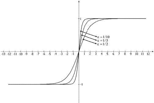
Figure 1: Graph of the sigmoid function for different $\varepsilon$ values.

$$\frac{d^{q}x}{dt^{q}}\in g(x)+A~{}S(x),~{}x(0)=x_{0},~{}\text{for a.a.~{}}t\in I,$$ (8)

Definition 1

[3],[22] selection of a set-valued function $F:\mathbb{R}^{n}\rightrightarrows\mathbb{R}^{n}$ is a single-valued function $f:\mathbb{R}^{n}\longrightarrow\mathbb{R}^{n}$ satisfying

$$h(x)\in F(x),~{}~{}\forall x\in\mathbb{R}^{n}.$$

Convex set-valued functions admit approximate selections [3], i.e. single-valued functions $h_{\varepsilon}:\mathbb{R}^{n}\longrightarrow\mathbb{R}^{n}$ for which $Graph(h_{\varepsilon})\subset Graph(F)+\varepsilon B~{}$and $h_{\varepsilon}(x)$ belongs to the convex hull of the image of $F.~{}$

Theorem 2

The set-valued function $AS~{}$ in the I.V.P. (8) admits a locally Lipschitzean approximate selection $h_{\varepsilon}:\mathbb{R}^{n}\longrightarrow\mathbb{R}^{n}$.

Proof Because $AS$ is upper semicontinuous with closed convex values (Remark 2), according to Cellina’s Theorem ( [3] p. 358, T. 9.2.1) it admits an approximate locally Lipschitz selection.

The constructive proof of Cellina’s theorem (see e.g. [2]) is a great advantage because it allows the construction of $h_{\varepsilon}~{}$.

There are several strategies to choose selections for a general class of set-valued problem (see e.g. [22]).

Following the preceding theorem, we can enounce the following main result

Proposition 3

Let the I.V.P. (3) with $g$ continuous. Then, the I.V.P. can be approximated by the following continuous I.V.P. of fractional-order

$$\frac{d^{q}x}{dt^{q}}=f(x),~{}~{}x(0)=x_{0},~{}~{}t\in I,$$

with $f:\mathbb{R}^{n}\longrightarrow\mathbb{R}^{n}$

$$f(x)=\left\{\begin{array}[]{c}g(x)+h_{\varepsilon}(x)~{}~{}\text{for~{}}x\in M\text{~{},}\\ g(x)+As(x)~{}~{}\text{for~{}}x\notin M,\end{array}\right.$$

where$~{}h_{\varepsilon}$ is an approximate selection of the set-valued function $AS.$

Proof

The proof is obvious if we consider that first, the I.V.P. (3) is transformed, via Filippov regularization, in the set-valued I.V.P. (8). Next, Theorem 2 can be applied in the neighborhoods of the discontinuity points.

Remark 3

i) Obviously, $\varepsilon$ is a vector and in applications we have chosen the same value for all its components;;
ii) As proved in [23], this local approximation can be made even with smooth functions;
iii) The proof of the above theorem could also be done via maximal monotonicity of $AS$ which ensures its closedness and convexity (see e.g. [2] p.141, Proposition 2).

Because of the amount of necessary calculus for fractional numerical integration, we shall use a simple form for $h_{\varepsilon}$.

To be precise, let us consider one component of $As$ in the I.V.P. (3), the scalar function $s_{j}(x_{j})=a_{ij}sgn(x_{j}).$ In a $\varepsilon-$neighborhood of $x_{j}$,  we have chosen in our numerical experiments for $h_{\varepsilon}$ the known sigmoid function, widely used in practical applications. Its scalar variant has the following form ( Fig. 1)

$$h_{\varepsilon}\left(x\right)=\frac{2}{1+e^{-x/\varepsilon}}-1.$$

To connect continuously $h_{\varepsilon}~{}$in some $\varepsilon-$neighborhood of $x_{j},~{}$we shall use the following form

$$h_{\varepsilon}\left(x_{j}\right)=\frac{2a_{ij}}{1+e^{-x_{j}/\varepsilon}}-a_{ij}.$$ (9)

The influence of $\varepsilon~{}$is underlined in Fig. 2 d and Fig. 2 e, where the visible (for $\varepsilon=1E-2$) corners, typical for discontinuous d.s., become smooth if the width of the neighborhood enlarges. Therefore, for physical reasons $\varepsilon$ needs to be chosen relatively small.

Conclusion The discontinuity hyperplanes of I.V.P. (3) can be replaced in their $\varepsilon$-neighborhoods with continuous surfaces, via approximate selections.

3 Numerical approach of discontinuous systems of fractional-order

In this section we present summarily a numerical scheme for continuous differential equations of fractional-order which will be used for our I.V.P.(3).

3.1 Numerical integration of differential equations of fractional-order

There are several definitions of the fractional differential operator.

The Caputo fractional derivative of order $q>0,$ where $q\in(m-1,m]$ for some $m\in\mathbb{N}$ for a differential function $x:[0,t]\longrightarrow\mathbb{R}$, is the most common tool, widely used in real applications, allowing for interpretation in a physically meaningful way (see e.g. [4], [15] and [24])

$$D^{q}x=\frac{1}{\Gamma(m-q)}\int\limits_{0}^{t}\frac{x^{(m)}(s)}{(t-s)^{q+1-m}}ds,$$

where $\Gamma$ is the known Gamma function.

To be precise, let us consider in the sequel the continuous autonomous fractional I.V.P.

$$\begin{array}[]{l}D^{q}x=f(x),\text{ }0\leq t\leq T,\text{ }x^{(k)}(0)=x_{0}^{(k)},\\ \text{ }k=0,1,\ldots,m-1.\end{array}$$ (10)

Table 1: Pseudo-code of DFF numerical scheme

$x_{i}[0]=x_{i0}[0],~{}i=1,2,\ldots,N_{e}$          {initial conditions} for $\text{ }j:=1\text{ }$to$~{}N~{}$do begin          for$\text{ \ }i:=1~{}$to$~{}N_{e}~{}$do                       {predictor} $\ \ \ \ \ \ \ \ \ \ \ \ \ \ \ \ \ p_{i}:=~{}x_{i0}[0]+\dfrac{h^{q}}{\Gamma(q+1)}\sum\limits_{k=0}^{j-1}b\left[j-k\right]f_{i}\left(x_{1}\left[k\right],\ldots,x_{N_{e}}\left[k\right]\right)~{}~{}\ \ \ \ \ \ \ \ \ \$          for $i:=1$ to $N_{e}$ do                                             {corrector} $\ \ \ \ \ \ \ \ \ \ \ \ \ \ \ \ \ x_{i}\left[j\right]:=x_{i~{}0}[0]+\dfrac{h^{q}}{\Gamma(q+2)}f_{i}(p_{1},\ldots,p_{N_{e}})+(\left(j-1\right)^{q+1}-\ \left(j-1-q\right)j^{q})f\left(x_{1}\left[0\right],\ldots,x_{N_{e}}\left[0\right]\right)$            $\ \ \ \ \ \ \ \ \ \ \ \ \ \ +\sum\limits_{k=1}^{j-1}a\left[j-k\right]f\left(x_{1}\left[k\right],\ldots,x_{N_{e}}\left[k\right]\right)$ end

Under the continuity condition of the function $f$, there is at least a solution (see e.g. [4] where the most general case of nonautonmous problems can be considered). Because $D^{q}$ has an $m$-dimensional kernel ($m~{}$being just the value rounded up to the nearest integer i.e. $m=\lceil q\rceil)$, $m$ initial conditions need to be specified. Certainly, for the usual case $0<q\leq 1$ we have to specify just one condition.

The fractional differential operators are computationally time expensive as compared to their integer-order counterparts. Some numerical methods for (10), essentially ad hoc methods for very specific types of differential equations are presented e.g. in [15], [25, 26, 27].

In agreement with the standard mathematical theory ([28] Sect. 42), the initial conditions for the I.V.P. (10) should have the form

$$\frac{d^{q-k}}{dt^{q-k}}x\left(t\right)|_{0_{+}}=b_{k},~{}~{}~{}k=1,\ldots,m.$$

However, because in practical applications, these values are frequently not available, and it may not even be clear what their physical meaning is, one can specify the initial conditions in the classical form as they are commonly used in initial value problems with integer-order equations [24].

The numerical scheme to integrate (10), which is used in this paper, is a predictor-corrector algorithm (called hereafter DFF), proposed by Diethlem, Ford and Freed in [4] together with error estimates and numerical examples. The scheme is a generalization of the classical multistep method Adams–Bashforth–Moulton and uses the Caputo derivative.

Being of practical significance and helpful for solving a broad class of problems, the method has been constructed and analyzed for the fully general set of equations without any special assumptions, and is easy to implement on a computer

Let us next assume that we are working on a uniform grid $\{t_{n}=nh:n=0,1,...,N\}$ with some integer $N$ with the step size $h:=T/N$ and the case of $q\in(0,1].$

The predictor formula for   the value at the point $t_{n+1},x^{p},$ is the fractional variant of the Adams-Bashforth method which for our particular case $m=1$, has the expression

$$x^{p}\left(t_{n+1}\right)=x_{0}+\frac{1}{\Gamma\left(q\right)}\sum\limits_{j=0}^{n}b_{j,n+1}f\left(x\left(t_{j}\right)\right),$$

while the corrector formula (the fractional variant of the one-step implicit Adams Moulton method)

$$x\left(t_{n+1}\right) = x_{0}+\frac{h^{q}}{\Gamma(q+2)}f\left(x^{p}\left(t_{n+1}\right)\right)$$

$$+\frac{h^{q}}{\Gamma(q+2)}\sum\limits_{j=0}^{n}a_{j,n+1}f\left(x\left(t_{j}\right)\right),$$

where $\Gamma$ is the Gamma function, and $a$ and $b$ are the corrector and predictor weights respectively given by the following formula

$$a_{j,n+1}=\left\{\begin{array}[]{ll}n^{q+1}-\left(n-q\right)\left(n+1\right)^{q}&\text{if }j=0,\\ \left(n-j+2\right)^{q+1}+\left(n-j\right)^{q+1}\\ -2\left(n-j+1\right)^{q+1}&\text{if }1\leq j\leq n,\\ 1&\text{if}~{}j=n+1,\end{array}\right.$$ (11)

and

$$b_{j,n+1}=\frac{h^{q}}{q}\left(\left(n+1-j\right)^{q}-\left(n-j\right)^{q}\right).$$ (12)

After a few modifications, designed to enhance the efficiency [4], DFF scheme has the form presented as pseudo-code in Table 1 for the case $m=1~{}$ and a set of $N_{e}~{}$autonomous differential equations of fractional-order $q$ with the right-hand side

$\left(f_{1}\left(x_{1},x_{2},\ldots,x_{N_{e}}\right),\ldots,\text{~{}}f_{N_{e}}\left(x_{1},x_{2},\ldots,x_{N_{e}}\right)\right)^{t}$

where:

$x_{i0},~{}i=1,2,...,N_{e}$ are the initial conditions;

$x[\cdot]$ array of $N+1$ real numbers containing the approximate solutions: $x_{k}$ $\thickapprox x(kh),$ $x$ being the exact solution;

$p$ the predicted values;

$a,b,$ arrays of $3\times(N+1)$ real numbers which, in this algorithm, are determined with the following variant [4].

for $k:=1~{}$to$~{}N~{}$do

$\ \ \ \ a[k]:=k^{q}-\left(k-1\right)^{q}$

$\ \ \ \ b[k]:=\left(k+1\right)^{q+1}-2k^{k+1}+\left(k-1\right)^{q+1}$

end

The Gamma function $\Gamma~{}$can be approximated via the so-called Lanczos approximation [29] using the formula (http://www.rskey.org/gamma.htm)

$$\Gamma(z)=\frac{\sum\limits_{i=0}^{6}P_{i}z^{i}}{\prod\limits_{i=0}^{6}(z+i)}(z+5.5)^{z+0.5}e^{-(z+5.5)},$$ (13)

for a complex variable $z$ for which $Re(z)>0$. The coefficients $P$ are drawn in Table 2

Table 2: $P$ coefficients for $\Gamma$ function (13)

$P_{0}=75122.6331530$

$P_{1}=80916.6278952$

$P_{2}=36308.2951477$

$P_{3}=8687.24529705$

$P_{4}=1168.92649479$

$P_{5}=83.8676043424$

$P_{6}=2.50662827511$

Remark 4

i) Another way to deal with fractional derivatives is the use of the frequency domain approximation, based on the approximation of the fractional operators in the frequency domain. This technique, proposed by researchers on automatic control, is suitable for Simulink (Matlab) (see e.g.[30, 31, 32]);
ii) As known, an attractor requires a relatively large integration time interval (for example for some of our experiments one needs $N=2E4\div 2.5E4$), and an array of this size is hard to implement in any compilers. The best solution we found for our examples was to save $x$ into a file.

3.2 Numerical integration of I.V.P. (3)

Now, using the results in Section 2 and Subsection 3.1, we can enounce the main result of this paper

Theorem 4

Let I.V.P. (3) with $g$ continuous. Then the problem can be numerically integrated.

Proof

The I.V.P. (3) can be transformed into a set-valued I.V.P., via Filippov s regularization (Section 2) which can be continuously approximated (Proposition 3). The obtained single-valued I.V.P. may be numerically integrated via DFF (Section 3.1).

One of the most unpleasant aspects of the DFF scheme is that it requires each step, the entire backward integration history. In other words, each value $x_{k}$ is a determined function of all previous values $x_{0},$ $x_{1},\ldots,x_{k-1}$

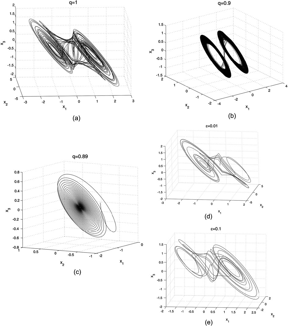
Figure 2: Phase plots for fractional discontinuous Sprott system (14). a),b) Chaotic trajectories for $q=1$ and $q=0.9.$ c) Attractive fixed point for $q=0.89.$ d) A chaotic trajectory for $q=0.95$ and $\varepsilon=0.01$ e) A chaotic trajectory for $q=0.95$ and $\varepsilon=0.1$.

or, for a large $k$, this implies supplementary computational cost. Thus, unlike the classical derivatives of integer order, the fractional derivatives operators are not local (i.e. we cannot determine $D^{q}x(t)$ by using only a few values of $x$ in a neighborhood of $t$).

Remark 5

Lipschitz continuity of $g$ is necessary only to ensure the uniqueness either of the I.V.P. (7 ) or (3) if the study of convergence properties and errors of some numerical method is required.

Error analysis is a difficult task, especially because of the numerical integration of fractional equations (see a detailed study in [24]). Therefore, in our study we have chosen empirically $h$ so that, for the common case $q=1$, the obtained attractor fits as well possible the known attractor shape in the phase space $\mathbb{R}^{3}$. Also, the optimal choice of the step length must ensure the maximum accuracy in the approximate solution at minimum computational cost.

In order to avoid the specific phenomena for discontinuous d.s. in the discontinuity surfaces (e.g. sliding modes [10]), the initial conditions need to be chosen in $D_{i}.~{}$As can be seen from the obtained images, the trajectories present some ”corners” typical of discontinuous d.s.

4 Examples

Let us first introduce the following notion

Notation Let us denote by $d=3q$ the order of the d.s. modeled by I.V.P. 3 and by $d^{*}$ the lowest value for which chaos persists.

While in the case of the continuous d.s. of integer-order chaos can appear only in nonlinear systems with order minimum 3, in nonlinear systems of fractional-order, this is not the case. For example, in [33] has been shown that a Chua circuit of order $d$ as low as 2.7 can produce a chaotic attractor; in [34] it is shown that a sinusoidally nonautonomous driven Duffing system with $d$ less than 2 can still behave in a chaotic manner; in [35] it is proved that the lowest order $d$ for fractional Lorenz system is $d^{*}=2.97$ and in [36] it is proved that the lowest-order chaotic system out of all the found chaotic systems reported in specialized literature, appears in the fractional Lü system.

In this section we explore the chaos disappearance, by searching $d^{*}$ with the algorithm proposed before, in two examples, of known discontinuous three-dimensional d.s. In the simulations, we only vary the fractional derivative order $q$ while the control parameter $p$ is fixed so the underlying d.s. of integer order behaves chaotically. Simulations are performed by lowering $q$ from $q=1~{}$(the integer case) until chaos behavior disappears.

All computations in this paper were performed in double precision arithmetic, $N$ was chosen large enough (of order $10E4$) to provide accurate results, the integration step size $h$ of $1E-3~{}$and $\varepsilon=1E-3$ of order.

Remark 6

In all the practical examples we have found in the scientific texts  (either two-dimensional, typical for dry friction problems, or three-dimensional, found generally in many areas of science) there is at most one $signum$ function in each equation of I.V.P. This helps to facilitate the numerical integration (as well known, it is time-consuming to compute the exponential functions).

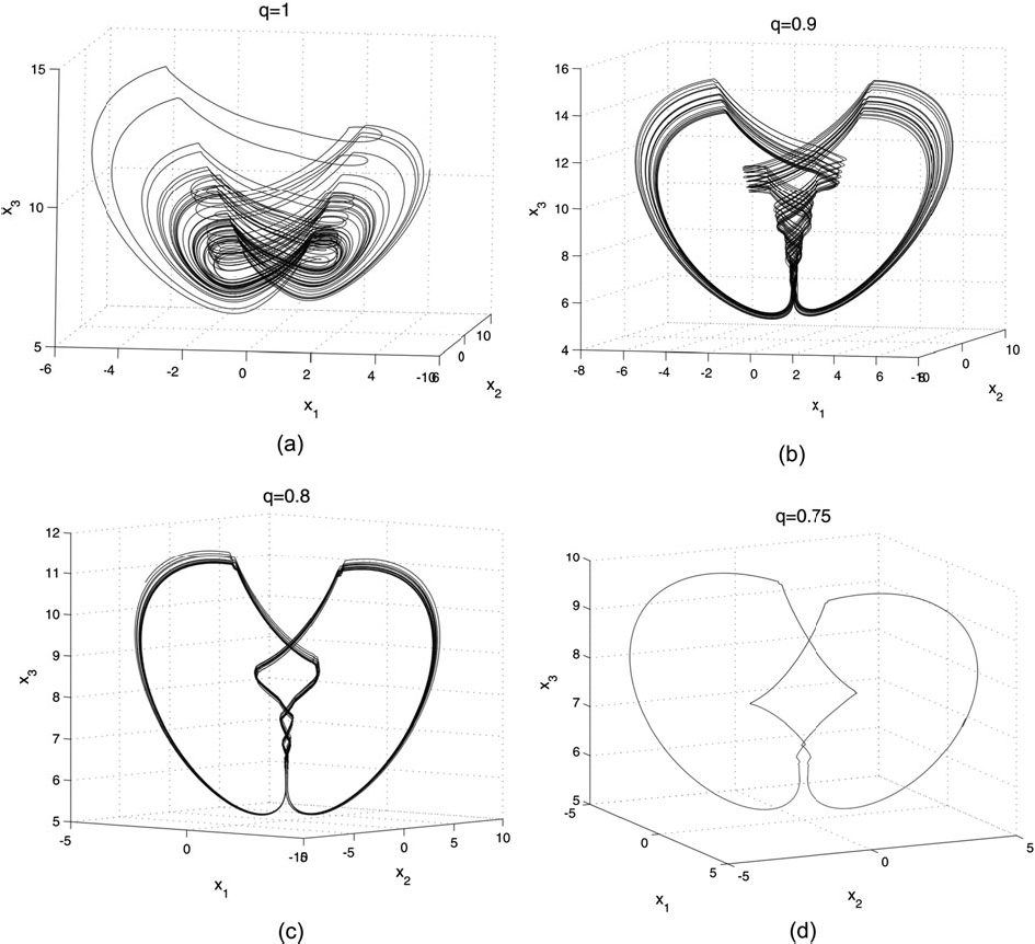
Figure 3: Phase plots for fractional discontinuous Chen system (15). a)-c) Chaotic trajectories for $q=1,~{}q=0.9$ and$~{}q=0.8$ respectively. d) Stable limit cycle for $q=0.75.$

4.1 Sprott system

The first example considered in this paper was proposed by Sprott in [32] and [38] and it is a representative one for the considered class of d.s.

$$\frac{d^{q}x_{1}}{dt^{q}} = x_{2},$$ (14)

$$\frac{d^{q}x_{2}}{dt^{q}} = x_{3},$$

$$\frac{d^{q}x_{3}}{dt^{q}} = -x_{1}-x_{2}-px_{3}+sgn(x_{1}).$$

whith

$$g(x)=\left(\begin{array}[]{c}x_{2}\\ x_{3}\\ -x_{1}-x_{2}-px_{3}\end{array}\right),\text{ }A=\left(\begin{array}[]{ccc}0&0&0\\ 0&0&0\\ 1&0&0\end{array}\right).\text{ }$$

In this case, the chaos corresponding to $p=0.5$ (see Fig. 2 a for $q=1$ and Fig. 2 b for $q=0.9$) vanishes at $q=0.89~{}$ when $d^{*}=2.57$ and when an attractive fixed point is obtained (Fig. 2 c).

4.2 Chen system

The next example is the fractional variant of the discontinuous Chen system [37] belonging to a more general class of discontinuous fractional systems

$$\frac{d^{q}x_{1}}{dt^{q}} = -p(x_{2}-x_{1}),$$ (15)

$$\frac{d^{q}x_{2}}{dt^{q}} = sgn(x_{1})(7-p-x_{3})+0.7x_{2},$$

$$\frac{d^{q}x_{3}}{dt^{q}} = sgn(x_{2})x_{1}-0.168x_{3}.$$

For $q=1$ the attractor (chaotic for $p=1.18$) is presented in Fig. 3 a. In this chase chaos seems to be more ”persistent” (see Fig. 3 b,c) since it exists until $q=0.75$ (see Fig. 3 d) when a stable limit cycle appears. Thus, $d^{*}=2.25$.

Conclusion In this paper, a continuous approximation, via Filippov regularization, of a class of fractional-order discontinuous I.V.P. has been considered. The obtained I.V.P. of fractional-order was integrated by using the algorithm proposed by Diethlem, Ford and Freed in [4]. Discontinuous fractional-order Sprott and Chen systems have been considered. We have found that chaos still exists in these systems if the order is lower than three. In the cases of continuous fractional systems, the chaotic behavior is affected when the fractional-order decreases. However, in our opinion, choosing the optimal value for $q$ (and implicitly for $d$), so that the mathematical model (3) can better illustrate the behavior and properties of a physical system, is much more important than finding the lowest $d^{*}$ (a simple reason could be that for $d=d^{*}$ chaos seems to vanish, in possible contradiction with the real system).

References

- [1] Filippov, A.F.: Differential Equations with Discontinuous Right-Hand Sides. Kluwer Academic Publishers, Dordrecht (1988)
- [2] Aubin, J.-P., Cellina, A.: Differential inclusions set-valued maps and viability theory. Springer, Berlin (1984)
- [3] Aubin, J.-P., Frankowska, H.: Set-valued analysis. Birkhuser, Boston (1990)
- [4] Diethelm, K., Ford, N.J. Freed, A.D.: Predictor-Corrector Approach for the Numerical Solution of Fractional Differential Equations. Nonlinear Dynamics 29, 3-22 (2002)
- [5] Andronov, A.A, Vitt A.A, Khaikin, S.E.: Theory of oscillators. Pergamon Press, Oxford (1966)
- [6] Buhite, J.L., Owen, D.R.: An ordinary differential equation from the theory of plasticity. Arch. Ration. Mech. Anal. 71, 357-383 (1979)
- [7] Clarke, F.H.: Optimization and non-smooth analysis. Wiley, New York (1983)
- [8] Deimling K.: Multivalued differential equations and dry friction problems. In: Fink, A.M., Miller, R.K., Kliemann W., editors. Proc. conf. Delay and Differential Equations, pp. 99-106. World Scientific, Singapore (1992)
- [9] Schilling, K.: An algorithm to solve boundary value problem for differential equations and applications in optimal control. Numer. Funct. Anal. Optim. 10, 733-764 (1989)
- [10] Wiercigroch, M:, de Kraker B. Applied nonlinear dynamics and chaos of mechanical systems with discontinuities. World Scientific, Singapore (2000)
- [11] Bagley, R.L., Calico, R.A.: Fractional order state equations for the control of viscoelastically damped structures. J. Guid. Control Dynam. 14, 304-311 (1991)
- [12] Nakagava, M., Sorimachi, K.: Basic characteristics of a fractance device. IEICE T. Fund. Electr. E75-A(12), 1814-1818 (1992)
- [13] Oustaloup, A.: La Derivation Non Entiere: Theorie, Synthese et Applications. Hermes, Paris (1995)
- [14] Sun, H.H., Abdelwahad, A.A., Onaral, B.: Linear approximation of transfer function with a pole of fractional order. IEEE Trans. Automat. Contr. 29,441-444 (1984)
- [15] Podlubny, I.: Fractional Differential Equations. Academic Press, San Diego (1999)
- [16] Ichise, M., Nagayanagi Y., Kojima, T.: An analog simulation of noninteger order transfer functions for analysis of electrode process. J. Electroanal Chem, 33, 253-265 (1971)
- [17] Podlubny, I., Petráš, I., Vinagre, B.M., O’Leary, P., Dorcák, L’.: Analogue realization of fractional-order controllers. Nonlinear Dyn. 29(1-4), 281-296 (2002)
- [18] Laskin, N.: Fractional market dynamics. Physica A 287, 482-492 (2000)
- [19] Kusnezov, D., Bulgac, A., Dang, G.D.: Quantum Levy processes and fractional kinetics. Phys. Rev. Lett. 82, 1136-1139 (1999)
- [20] Taubert, K.: Converging multistep Methods for Initial Value Problems Involving Multivalued Maps. Computing 27, 123-136 (1981)
- [21] Dontchev, A. and Lempio, F.: Difference Methods for Differentiale Inclusions. SIAM Rev., 34, 263-294 (1992)
- [22] Kastner-Maresch A., Lempio F.: Difference methods with selection strategies for differential inclusions. Numer. Funct. Anal. Optimiz. 14, 555-572 (1993)
- [23] Danca M.-F., Codreanu, S.: On a possible approximation of discontinuous dynamical systems. Chaos, Solitons & Fractals 13, 681-691 (2002)
- [24] Diethelm, K., Ford, N.J.: Analysis of Fractional Differential Equations. Journal of Mathematical Analysis and Applications 265, 229-248 (2002)
- [25] Diethelm, K.: An algorithm for the numerical solution of differential equations of fractional order. Electronic Transactions on Numerical Analysis 5, 1-6 (1997)
- [26] Lubich, C.: Discretized fractional calculus. SIAM Journal on Mathematical Analysis 17, 704-719 (1986)
- [27] Shokooh, A., Suarez, L.E.: A comparison of numerical methods applied to a fractional model of damping materials. J. Vib. Control, 5, 331-354 (1999)
- [28] Samko, S. G., Kilbas, A. A., Marichev, O. I.: Fractional Integrals and Derivatives: Theory and Applications. Gordon and Breach, Yverdon, (1993)
- [29] Press, W.H., Teukolsky, S.A., Vetterling, W.T., Flannery, B.P.: Numerical Recipes in C, The Art of Scientific Computing, Second Edition. Cambridge University Press, (1992)
- [30] Charef, A. Sun, H.H., Tsao, Y.Y. Onaral, B.: Fractal system as represented by singularity function. IEEE T. Automat. Contr. 37, 1465-1470 (1992)
- [31] Petráš, I.: Chaos in the fractional-order Volta’s system: modeling and simulation. Nonlinear Dynam. 57(1-2), 157-170 (2009)
- [32] Ahmad, W.M., Sprott, J.C.: Chaos in fractional-order autonomous nonlinear systems. Chaos, Solitons and Fractals 16, 339-351 (2003)
- [33] Hartley, T.T., Lorenzo, C.F., Qammer, H.K.: Chaos in a fractional order Chua’s system. IEEE T. Circuits-I 42(8), 485-490 (1995)
- [34] Arena, P., Caponetto, R., Fortuna, L., Porto, D.: Chaos in a fractional order Duffing system. In: Proceedings ECCTD, Budapest, September, 1259-1262 (1997)
- [35] Wu, X.-J., Shen, S.-L.: Chaos in the fractional-order Lorenz system. International Journal of Computer Mathematics 86(7), 1274-1282 (2009)
- [36] Lu, J.G.: Chaotic dynamics of the fractional-order Lü system and its synchronization. Physics Letters A 354, 305-311 (2006)
- [37] Aziz-Alaoui, M.A., Chen, G.: Asymptotic Analysis of a New Piecewise-Linear Chaotic System. Int. J. Bifurcat. Chaos 12(1), 147-157 (2002)
- [38] Sprott, J.C.: A New Class of Chaotic Circuit. Physics Letters A, 266, 19-23 (2000)