Higher twist parton distributions from light-cone wave functions

Abstract

We explore the possibility to construct higher-twist parton distributions in a nucleon at some low reference scale from convolution integrals of the light-cone wave functions (WFs). To this end we introduce simple models for the four-particle nucleon WFs involving three valence quarks and a gluon with total orbital momentum zero, and estimate their normalization (WF at the origin) using QCD sum rules. We demonstrate that these WFs provide one with a reasonable description of both polarized and unpolarized gluon parton densities at large values of Bjorken variable $x\geq 0.5$. Twist-three parton distributions are then constructed as convolution integrals of $qqqg$ and usual three-quark WFs. The cases of the polarized structure function $g_{2}(x,Q^{2})$ and single transverse spin asymmetries are considered in detail. We find that the so-called gluon-pole contribution to twist-three distributions relevant for single spin asymmetry vanishes in this model, but is generated perturbatively at higher scales by the evolution, in the spirit of GRV parton distributions.

I Introduction

Higher-twist parton distributions are conceptually very interesting as they go beyond the simple parton model description and allow one to quantify correlations between the partons. Unfortunately, they prove to be very elusive. Despite considerable efforts, very little is known even about the simplest, twist-three distributions which contribute, e.g. structure function $g_{2}(x,Q^{2})$ in the polarized deep-inelastic scattering Efremov:1983eb ; Bukhvostov:1984as ; Ratcliffe:1985mp ; Balitsky:1987bk ; Balitsky:1989jb ; Ali:1991em ; Kodaira:1996md ; Kodaira:1998jn ; Accardi:2009au and transverse single spin asymmetries (SSAs) in the collinear factorization approach Efremov:1981sh ; Efremov:1984ip ; Qiu:1991pp ; Qiu:1991wg ; Efremov:1994dg ; Qiu:1998ia ; Kanazawa:2000hz ; Kanazawa:2000cx ; Eguchi:2006mc ; Koike:2007rq ; Kang:2008ih .

One general reason for this is that the structure of higher twist parton distributions is much more complicated compared to the leading twist: they are functions of two and more parton momentum fractions. The usual strategy to extract parton distributions from experimental data has been to assume a certain functional form with a few adjustable parameters at a reference scale, and find the parameters by making global fits to the available data. This is a standard approach which works quite well for the leading twist. Unfortunately, it does not work for higher twist (or, at least, has not been applied systematically) because there is no physical intuition on how such distributions may look like. Also the asymptotic behavior of higher-twist distributions both at small and large $x$ is poorly understood. Hence it is very hard to guess an adequate parametrization.

In this work we make a step in this direction. Recall that the case of higher-twist parton distributions is not unique in that they are functions of several kinematic variables: in studies of generalized parton distributions (GPDs) or “unintegrated” transverse-momentum dependent distributions (TMDs) the same complication arises. In both cases, representations in terms of overlap integrals of light-cone wave functions have been extremely useful for developing the underlying physics picture and provide one with a good basis for theoretical modelling. In what follows we try to follow the same path for the construction of higher-twist distributions as overlap integrals between Fock states with the minimum (valence) and next-to-minimum (one extra gluon) parton content.

In order to keep the model as simple as possible, in this work we restrict ourselves to contributions of the states with total zero angular momentum. We overtake the expressions for three-quark wave functions from Ref. Diehl:1998kh which have been shown Bolz:1996sw ; Diehl:1998kh to provide one with a good description for quark parton densities at large $x$ and the nucleon magnetic form factor. The new contribution of this paper is to include into consideration the Fock states with one additional gluon which were considered in Diehl:1998kh on a qualitative level. We find that there exist three independent $qqqg$ wave functions with zero orbital momentum. Our analysis of their symmetry properties does not agree with earlier results Ji:2003yj . We calculate the normalization of these new wave functions using QCD sum rule approach and construct explicit models by the requirement that their light-cone limit (zero transverse separation) reproduces the nucleon twist-4 distribution amplitudes introduced in Ref. Braun:2008ia .

Having specified the wave functions, we calculate the quark and gluon polarized and unpolarized parton distributions and find agreement with the existing parametrizations at large $x$ without any fine-tuning of the parameters. Encouraged by this, we construct the twist-three correlation function involving a quark, antiquark and gluon fields which is relevant for the structure function $g_{2}(x,Q^{2})$ and single spin asymmetries. In our model this correlation function vanishes at the boundaries of parton regions where one of the momentum fractions goes to zero, but non-zero values are obtained at higher scales perturbatively through the QCD evolution. This phenomenon is in full analogy to the generation of a large gluon parton distribution at small $x$ starting from the “valence”-like ansatz in the GRV approach Gluck:1994uf ; Gluck:1998xa . Such, radiatively generated, soft-gluon pole and soft-fermion pole contributions to the spin asymmetries are calculated and compared to the existing parametrizations. The sign of radiatively generated soft pole terms as well as the sign of the twist-three contribution to the structure function $g_{2}(x,Q^{2})$ at large $x$ are largely model-independent predictions of our approach; these signs turn out to be in agreement with the data in all cases. Finally, we discuss possible generalizations of our simple model that may provide one with usable parametrizations for the phenomenological analysis.

II Light-cone coordinates

For an arbitrary four-vector $a^{\mu}$ we define the light-cone coordinates as

$$a_{+}=\frac{1}{\sqrt{2}}(a^{0}+a^{3})\,,\qquad a_{-}=\frac{1}{\sqrt{2}}(a^{0}-a^{3})\,,$$

$$a=a^{1}+ia^{2}\,,\hskip 46.94687pt\bar{a}=a^{1}-ia^{2}\,,$$ (1)

so that the matrix $a=a_{\mu}\sigma^{\mu}$, where $\sigma^{\mu}=(\mathbb{I},\vec{\sigma})$ takes the form

$$a_{\alpha\dot{\alpha}}=a_{\mu}\sigma^{\mu}_{\alpha\dot{\alpha}}=\begin{pmatrix}\sqrt{2}a_{-}&-\bar{a}\\ -a&\sqrt{2}a_{+}\end{pmatrix}.$$ (2)

In what follows we use Weyl representation for the $\gamma-$matrices

$$\gamma^{0}=\begin{pmatrix}0&\mathbb{I}\\ \mathbb{I}&0\end{pmatrix}\,,\qquad\gamma^{i}=\begin{pmatrix}0&\sigma^{i}\\ -\sigma^{i}&0\end{pmatrix}\,,$$

$$\gamma^{5}\equiv\gamma^{0}\gamma^{1}\gamma^{2}\gamma^{3}=\begin{pmatrix}-\mathbb{I}&0\\ 0&\mathbb{I}\end{pmatrix}\,$$ (3)

and the two-component notation for Dirac spinors

$$q=\begin{pmatrix}\psi_{\alpha}\\ \bar{\chi}^{\dot{\alpha}}\end{pmatrix}\equiv\begin{pmatrix}q_{\downarrow}\\ q_{\uparrow}\end{pmatrix}\,,\quad\bar{q}=q^{\dagger}\gamma^{0}=(\chi^{\alpha},\bar{\psi}_{\dot{\alpha}})\equiv(\bar{q}_{\downarrow},\bar{q}_{\uparrow})\,.$$ (4)

The two independent light-like vectors

$$n^{\mu}=\frac{1}{\sqrt{2}}(1,0,0,-1)\,,\qquad\tilde{n}^{\mu}=\frac{1}{\sqrt{2}}(1,0,0,1)\,,$$ (5)

$n^{2}=\tilde{n}^{2}=0$, $n\tilde{n}=1$ can be parametrized in terms of the two auxiliary Weyl spinors:

$$n_{\alpha\dot{\alpha}}=\lambda_{\alpha}\bar{\lambda}_{\dot{\alpha}}\,,\qquad\tilde{n}_{\alpha\dot{\alpha}}=\mu_{\alpha}\bar{\mu}_{\dot{\alpha}}\,,$$ (6)

where

$$\lambda_{\alpha}=2^{1/4}\begin{pmatrix}-1\\ 0\end{pmatrix}, \mu_{\alpha}=2^{1/4}\begin{pmatrix}0\\ 1\end{pmatrix},$$

$$\bar{\lambda}_{\dot{\alpha}}=2^{1/4}\begin{pmatrix}-1\\ 0\end{pmatrix}, \bar{\mu}_{\dot{\alpha}}=2^{1/4}\begin{pmatrix}0\\ 1\end{pmatrix}.$$ (7)

We accept the following rules for raising and lowering the spinor indices (cf. Ref. Braun:2008ia )

$$\lambda^{\alpha}=\epsilon^{\alpha\beta}\lambda_{\beta}\,,\quad\lambda_{\alpha}=\lambda^{\beta}\epsilon_{\beta\alpha}\,,\quad\bar{\lambda}^{\dot{\alpha}}=\bar{\lambda}_{\dot{\beta}}\epsilon^{\dot{\beta}\dot{\alpha}}\!\!,\quad\bar{\lambda}_{\dot{\alpha}}=\epsilon_{\dot{\alpha}\dot{\beta}}\bar{\lambda}^{\dot{\beta}}\!,$$ (8)

where the antisymmetric Levi-Civita tensor is defined as

$$\epsilon_{12}=\epsilon^{12}=-\epsilon_{\dot{1}\dot{2}}=-\epsilon^{\dot{1}\dot{2}}=1\,.$$

The auxiliary spinors $\lambda$ and $\mu$ are normalized as

$$(\mu\lambda)=\mu^{\alpha}\lambda_{\alpha}=-(\lambda\mu)=-\sqrt{2}\,,$$

$$(\bar{\mu}\bar{\lambda})=\bar{\mu}_{\dot{\alpha}}\bar{\lambda}^{\dot{\alpha}}=-(\bar{\lambda}\bar{\mu})=+\sqrt{2}\,$$ (9)

and serve to specify ”plus” and ”minus” components of the fields. We define

$$\psi_{+}=\lambda^{\alpha}\psi_{\alpha}, \psi_{-}=\mu^{\alpha}\psi_{\alpha},$$

$$\bar{\chi}_{+}=\bar{\chi}_{\dot{\alpha}}\bar{\lambda}^{\dot{\alpha}}, \bar{\chi}_{-}=\bar{\chi}_{\dot{\alpha}}\bar{\mu}^{\dot{\alpha}}\,,$$ (10)

so that each two-component spinor can be decomposed as

$$(\mu\lambda)\psi_{\alpha}=\lambda_{\alpha}\,\psi_{-}-\mu_{\alpha}\,\psi_{+}\,,$$

$$(\bar{\lambda}\bar{\mu})\bar{\chi}^{\dot{\alpha}}=\bar{\lambda}^{\dot{\alpha}}\,\bar{\chi}_{-}-\bar{\mu}^{\dot{\alpha}}\,\bar{\chi}_{+}\,.$$ (11)

In the same notation the light-cone decomposition of a vector (e.g. gluon) field takes the form

$$A_{\alpha\dot{\alpha}} =A_{-}\,\lambda_{\alpha}\bar{\lambda}_{\dot{\alpha}}+A_{+}\,\mu_{\alpha}\bar{\mu}_{\dot{\alpha}}+\frac{\bar{A}}{\sqrt{2}}\,\lambda_{\alpha}\bar{\mu}_{\dot{\alpha}}+\frac{A}{\sqrt{2}}\,\mu_{\alpha}\bar{\lambda}_{\dot{\alpha}}\,.$$ (12)

The ”plus” spinor fields $\psi_{+},\bar{\chi}_{+}$ and transverse gluon fields $A,\bar{A}$ are assumed to be the dynamical fields in the light-cone quantization framework. The ”minus” fields $\psi_{-},\bar{\chi}_{-},A_{-}$ can be expressed in terms of the dynamical ones with the help of equations of motion (EOM) whereas $A_{+}=0$ due to the gauge fixing condition.

The plus quark fields have the following canonical expansion

$$q_{\downarrow+}(x)= \int\!\frac{dp_{+}}{\sqrt{2p_{+}}}\frac{d^{2}p_{\perp}}{(2\pi)^{3}}\theta(p_{+})\biggl{[}e^{-ipx}b_{\downarrow}(p)+e^{+ipx}d_{\uparrow}^{\dagger}(p)\biggr{]},$$

$$q_{\uparrow+}(x)= \int\!\frac{dp_{+}}{\sqrt{2p_{+}}}\frac{d^{2}p_{\perp}}{(2\pi)^{3}}\theta(p_{+})\biggl{[}e^{-ipx}b_{\uparrow}(p)+e^{+ipx}d^{\dagger}_{\downarrow}(p)\biggr{]},$$ (13)

where $b_{\uparrow(\downarrow)},d_{\uparrow(\downarrow)}$ are the annihilation operators of quark and antiquark of positive (negative) helicity, respectively. They obey the standard anticommutation relations

$$\{b_{\lambda}(p),b_{\lambda^{\prime}}^{\dagger}(p^{\prime})\}=\{d_{\lambda}(p),d^{\dagger}_{\lambda^{\prime}}(p^{\prime})\}=$$ (14)

$$= 2p_{+}(2\pi)^{3}\delta_{\lambda,\lambda^{\prime}}\delta(p_{+}-p^{\prime}_{+})\delta^{2}(p_{\perp}-p^{\prime}_{\perp})\,.$$

The similar expansion for the dynamical transversely polarized gluon fields $A$ and $\bar{A}$ reads

$$\bar{A}(x) \!=\! \sqrt{2}\!\int\!\frac{dk_{+}}{2k_{+}}\frac{d^{2}k_{\perp}}{(2\pi)^{3}}\theta(k_{+})\biggl{[}e^{-ikx}a_{\uparrow}(k)+e^{+ikx}a_{\downarrow}^{\dagger}(k)\biggr{]},$$

$$A(x) \!=\! \sqrt{2}\!\int\!\frac{dk_{+}}{2k_{+}}\frac{d^{2}k_{\perp}}{(2\pi)^{3}}\theta(k_{+})\biggl{[}e^{-ikx}a_{\downarrow}(k)+e^{+ikx}a_{\uparrow}^{\dagger}(k)\biggr{]}.$$

(15)

Here and below $A=\sum_{a}t^{a}A^{a}$ etc. where $t^{a}$ are the usual $SU(3)$ generators in the fundamental representation, normalized as $tr(t^{a}t^{b})=\dfrac{1}{2}\delta^{ab}$. The creation and annihilation operators obey the commutation relation

$$\Big{[}a^{b}_{\lambda}(p),(a^{b^{\prime}}_{\lambda^{\prime}}(p^{\prime}))^{\dagger}\Big{]}=$$ (16)

$$= 2p_{+}(2\pi)^{3}\delta_{\lambda,\lambda^{\prime}}\delta^{bb^{\prime}}\delta(p_{+}-p^{\prime}_{+})\delta^{2}(p_{\perp}-p^{\prime}_{\perp})\,.$$

Finally, the gluon strength tensor $F_{\mu\nu}$ and its dual $\widetilde{F}_{\mu\nu}$ can be decomposed as

$$F_{\alpha\beta,\dot{\alpha}\dot{\beta}} =\sigma^{\mu}_{\alpha\dot{\alpha}}\sigma^{\nu}_{\beta\dot{\beta}}F_{\mu\nu}=2\Big{(}\epsilon_{\dot{\alpha}\dot{\beta}}f_{\alpha\beta}-\epsilon_{\alpha\beta}\bar{f}_{\dot{\alpha}\dot{\beta}}\Big{)}\,,$$

$$i{\widetilde{F}}_{\alpha\beta,\dot{\alpha}\dot{\beta}} =2\Big{(}\epsilon_{\dot{\alpha}\dot{\beta}}f_{\alpha\beta}+\epsilon_{\alpha\beta}\bar{f}_{\dot{\alpha}\dot{\beta}}\Big{)}\,.$$ (17)

Here $f_{\alpha\beta}$ and $\bar{f}_{\dot{\alpha}\dot{\beta}}$ are chiral and antichiral symmetric tensors, $f_{\alpha\beta}=f_{\beta\alpha}$, $\bar{f}=f^{*}$, which belong to $(1,0)$ and $(0,1)$ representations of the Lorenz group, respectively. Their ”good components” are defined as

$$f_{++}=\lambda^{\alpha}\lambda^{\beta}f_{\alpha\beta}\,, \bar{f}_{++}=\bar{\lambda}^{\dot{\alpha}}\bar{\lambda}^{\dot{\beta}}\bar{f}_{\dot{\alpha}\dot{\beta}}\,.$$ (18)

In the light-cone gauge

$$f_{++}=-\partial_{+}A\,,\qquad\bar{f}_{++}=-\partial_{+}\bar{A}\,,$$ (19)

where $\partial_{+}=n^{\mu}\partial_{\mu}=\partial/\partial x_{-}$, so that they can readily be expanded in contributions of annihilation and creation operators using Eq. (15).

As mentioned above, ”minus” field components can be expressed in terms of the dynamical fields using QCD equations of motion.

III Nucleon light-cone wave functions

III.1 Definitions and symmetry properties

The light-cone wave functions (LCWFs) are defined as probability amplitudes of the corresponding parton states which build up the proton with a given helicity. They depend on parton longitudinal momentum fractions $x_{i}$, transverse momenta $k_{\perp i}$, and on parton helicities. LCWFs are usually thought of as solutions of the eigenvalue problem for the light-cone quantized QCD Hamiltonian Kogut:1969xa ; Brodsky:1997de , although this construction is far from being complete.

Throughout this work we adopt some definitions and partially also the notation from Ref. Diehl:1998kh . In particular we use a shorthand notation for the $N$-parton differential phase space

$$[dx]_{N}= \prod_{i=1}^{N}dx_{i}\,\delta(1-\sum x_{i})\,,$$

$$[dk_{\perp}]_{N}= \frac{1}{(16\pi^{3})^{N-1}}\prod_{i=1}^{N}d^{2}k_{\perp,i}\,\delta^{2}\left(\sum k_{\perp i}\right)$$ (20)

and

$$[\mathcal{D}X]_{N}=\frac{1}{\sqrt{x_{1}\ldots x_{N}}}[dx]_{N}[dk_{\perp}]_{N}\,.$$ (21)

The valence three-quark state with zero angular momentum is the simplest one. It can be described in terms of the single LCWF Lepage:1980fj ; Diehl:1998kh

$$|{p,+}\rangle_{uud} = -\frac{\epsilon^{ijk}}{\sqrt{6}}\int[\mathcal{D}X]_{3}\Psi_{123}^{(0)}(X)\,$$

$${}\times\Bigl{(}u_{i\uparrow}^{\dagger}(1)u_{j\downarrow}^{\dagger}(2)d_{k\uparrow}^{\dagger}(3)-u_{i\uparrow}^{\dagger}(1)d_{j\downarrow}^{\dagger}(2)u_{k\uparrow}^{\dagger}(3)\Bigr{)}|{0}\rangle\,.$$

Here and below the argument of the field $u^{\dagger}_{i\uparrow}(1)$ etc. refers to the collection of its arguments that are not shown explicitly, i.e. $u^{\dagger}_{\uparrow i}(1)=u^{\dagger}_{\uparrow i}(x_{1},k_{\perp,1})$. The (real) function $\Psi_{123}^{(0)}(X)$ depends on momentum fractions $x_{i}$ and transverse momenta $k_{\perp,i}$ of all partons.

Models for $\Psi_{123}^{(0)}(X)$ of various degree of sophistication have been was considered in different context in a large number of papers see e.g. Refs. Lepage:1980fj ; Bolz:1994hb ; Bolz:1996sw ; Diehl:1998kh ; Ji:2003yj ; Pasquini:2008ax . In this work we adopt the simplest ansatz Diehl:1998kh

$$\Psi_{123}^{(0)}= \frac{1}{4\sqrt{6}}\,\phi(x_{1},x_{2},x_{3})\,\Omega_{3}(a_{3},x_{i},k_{\perp i})\,.$$ (23)

The transverse momentum dependence is contained in the function $\Omega_{N}$

$$\Omega_{N}(a_{N},x_{i},k_{\perp i})=\frac{(16\pi^{2}a_{N}^{2})^{N-1}}{x_{1}x_{2}\ldots x_{N}}\exp\left[-a_{N}^{2}\sum_{i}k_{\perp i}^{2}/x_{i}\right]\,$$ (24)

which is normalized such that

$$\int[d^{2}k_{\perp}]_{N}\Omega_{N}(a_{N},x_{i},k_{\perp i})\,=\,1\,,$$

$$\int[d^{2}k_{\perp}]_{N}\Omega^{2}_{N}(a_{N},x_{i},k_{\perp i})\,=\,\frac{\rho_{N}}{x_{1}\ldots x_{N}}\,,$$ (25)

where

$$\rho_{N}=(8\pi^{2}a_{N}^{2})^{N-1},$$

and $\phi(x_{i})$ is related to the leading-twist-3 nucleon distribution amplitude (see the next Section). The parameter $a_{3}$ determines the spread of the wave function in the transverse plane and e.g. the average quark transverse momentum.

The general classification of Fock states involving an additional gluon was given in Ref. Ji:2003yj . Unfortunately, we do not agree with the analysis in Ji:2003yj of the symmetry properties of the corresponding LCWFs.

As in the three quark case, we restrict ourselves to the states with zero total orbital angular momentum, $L_{z}=0$. There are two possibilities Ji:2003yj : either the quark helicities sum up to $\lambda_{uud}=3/2$ and the gluon has opposite helicity to that of the proton, $\lambda_{g}=-1$, or, alternatively, $\lambda_{uud}=-1/2$ and $\lambda_{g}=+1$. We begin with the first case.

The starting observation is that the $SU(3)$ generators obey the following identity

$$\epsilon^{ijl}t^{a}_{lk}+\epsilon^{ilk}t^{a}_{lj}+\epsilon^{ljk}t^{a}_{li}=0$$ (26)

As a consequence, there exists only one possibility to form a colorless state (up to equivalent redefinitions)

$$|{p,+}\rangle_{uudg_{\downarrow}} = \epsilon^{ijk}\int[\mathcal{D}X]_{4}\,\Psi^{\downarrow}_{1234}(X)\,$$ (27)

$${}\times g_{\downarrow}^{a,\dagger}(4)\,[t^{a}u_{\uparrow}(1)]_{i}^{\dagger}\,u^{\dagger}_{j\uparrow}(2)\,d_{k\uparrow}^{\dagger}(3)|{0}\rangle\,.$$

Note that $[t^{a}u_{\uparrow}(1)]_{i}^{\dagger}=u^{\dagger}_{i^{\prime}\uparrow}(1)\,t^{a}_{i^{\prime}i}$. Symmetry properties of the LCWF $\Psi^{\downarrow}_{1234}$ are determined by the requirement that the nucleon has isospin 1/2. Since $I_{3}=1/2$ is fixed by the quark flavor content, the $I=1/2$ requirement is equivalent to the simpler condition that the state is annihilated by the isospin step-up operator

$$I_{+}|{p,+}\rangle_{uudg_{\downarrow}}=0.$$

The action of $I_{+}$ amounts to the replacement of quark flavors $d\to u$ in (27), $I^{+}\sim u^{\dagger}{\delta}/{\delta d^{\dagger}}$. Projecting the resulting state onto $\langle{0}|g_{\downarrow}^{a^{\prime}}(4^{\prime})u_{k^{\prime}\uparrow}(3^{\prime})u_{j^{\prime}\uparrow}(2^{\prime})u_{k^{\prime}\uparrow}(1^{\prime})$ and collecting the terms in the two independent color structures (cf. Eq. (26)) one finds two constraints:

$$\Psi^{\downarrow}_{1234}+\Psi^{\downarrow}_{1324}-\Psi^{\downarrow}_{3124}-\Psi^{\downarrow}_{3214}=0\,,$$

$$\Psi^{\downarrow}_{2134}+\Psi^{\downarrow}_{2314}-\Psi^{\downarrow}_{3124}-\Psi^{\downarrow}_{3214}=0\,.$$ (28)

Since the second equation can be obtained from the first one by renaming $1\leftrightarrow 2$, only one of them is independent. In order to solve this constraint it is convenient to represent the function $\Psi^{\downarrow}$ as sum of contributions with definite parity under cyclic permutations of the first three (quark) arguments $123\to 231$:

$$\Psi^{\downarrow}_{1234}=\Psi^{\downarrow,0}_{1234}+\Psi^{\downarrow,+}_{1234}+\Psi^{\downarrow,-}_{1324}\,,$$ (29)

such that

$$\Psi^{\downarrow,0}_{1234}=\Psi^{\downarrow,0}_{2314}\,,\qquad\Psi^{\downarrow,\pm}_{1234}=e^{\pm 2\pi i/3}\Psi^{\downarrow,\pm}_{2314}.$$

One easily finds that an arbitrary function $\Psi^{\downarrow,0}_{1234}$ is a solution of Eq. (III.1) whereas one has to require that $\Psi^{\downarrow,-}_{1234}=-\Psi^{\downarrow,+}_{1324}$. Thus the most general solution to the isospin constraint can be written as

$$\Psi^{\downarrow}_{1234}=\Phi^{\downarrow,0}_{1234}+\Psi^{\downarrow,+}_{1234}-\Psi^{\downarrow,+}_{1324}\,,$$ (30)

where $\Psi^{\downarrow,0}$ and $\Psi^{\downarrow,+}$ are arbitrary functions with the specified symmetry under cyclic permutations.

Our result does not agree with the conclusion of Ji:2003yj that the function $\Psi^{\downarrow}_{1234}$ ($\psi^{(1)}_{uudg}$ in notations of Ref. Ji:2003yj ) is antisymmetric with respect to permutation of the second and third arguments, which is a much stronger condition. In fact any function which is antisymmetric in $2\leftrightarrow 3$ can indeed be written in the form (30). However, e.g. a totally symmetric function in the quark arguments is also allowed. The reason why this does not contradict isospin counting is that the corresponding state is annihilated by $I_{+}$ thanks to the color identity (26). We note in passing that the $SU(3)$-color generators in the definitions given in Ji:2003yj must be transposed, $t^{a}_{ii^{\prime}}\to t^{a}_{i^{\prime}i}$.

The second case, a gluon with positive helicity, can be treated similarly. There exist two independent LCWFs which can be defined as

$$|{p,+}\rangle_{uudg^{\uparrow}} = \epsilon^{ijk}\int[\mathcal{D}X]_{4}\Big{\{}\Psi^{\uparrow(1)}_{1234}(X)\,[t^{a}u_{\downarrow}(1)]_{i}^{\dagger}\Bigl{(}u_{j\uparrow}^{\dagger}(2)d_{k\downarrow}^{\dagger}(3)-d_{j\uparrow}^{\dagger}(2)u_{k\downarrow}^{\dagger}(3)\Bigr{)}g_{\uparrow}^{a,\dagger}(4)$$ (31)

$${}\hskip 28.45274pt+\Psi^{\uparrow(2)}_{1234}(X)u^{\dagger}_{i\downarrow}(1)\Big{(}[t^{a}u_{\downarrow}(2)]^{\dagger}_{j}\,d^{\dagger}_{k\uparrow}(3)-[t^{a}d_{\downarrow}(2)]^{\dagger}_{j}\,u^{\dagger}_{k\uparrow}(3)\Big{)}g_{\uparrow}^{a,\dagger}(4)\Big{\}}|{0}\rangle\,.$$

The functions $\Psi^{\uparrow(1)}_{1234}$ and $\Psi^{\uparrow(2)}_{1234}$ have no symmetry constraints. This result also does not agree with Ji:2003yj .

In what follows we accept the following ansatz for the quark-gluon LCWFs

$$\Psi^{\downarrow}_{1234}= \frac{1}{\sqrt{2x_{4}}}\phi_{g}(x_{1},x_{2},x_{3},x_{4})\,\Omega_{4}(a_{g}^{\downarrow},x_{i},k_{\perp i})\,,$$

$$\Psi^{\uparrow(1)}_{1234}= \frac{1}{\sqrt{2x_{4}}}\psi_{g}^{(1)}(x_{1},x_{2},x_{3},x_{4})\,\Omega_{4}(a_{g}^{\uparrow},x_{i},k_{\perp i})\,,$$

$$\Psi^{\uparrow(2)}_{1234}= \frac{1}{\sqrt{2x_{4}}}\psi_{g}^{(2)}(x_{1},x_{2},x_{3},x_{4})\,\Omega_{4}(a_{g}^{\uparrow},x_{i},k_{\perp i})\,.$$ (32)

The function $\Omega_{4}$ is defined in Eq. (24) and the momentum fraction distributions $\phi_{g}(x_{i})$, $\psi_{g}^{(1,2)}(x_{i})$ are related to the next-to-leading twist-4 nucleon distribution amplitudes as discussed in the next section. For simplicity we choose the same parameter $a_{g}^{\uparrow}$ determining the spread of both wave functions $\Psi^{\uparrow(1)}$ and $\Psi^{\uparrow(2)}$ in the transverse plane. This restriction can be relaxed.

III.2 Relation to nucleon distribution amplitudes

Nucleon distribution amplitudes (DAs) are defined as LCWFs with all constituents at small transverse separations, schematically Lepage:1980fj

$$\phi(x_{i},\mu)\sim\int^{|k_{\perp}|<\mu}[dk_{\perp}]_{N}\,\Phi_{N}(x_{i},k_{\perp,i})\,.$$ (33)

As always in a field theory, taking an asymptotic limit (here vanishing transverse distance) produces divergences that have to be regularized. Hence DAs are scale-dependent objects which only include contributions of small transverse momenta, less that the cutoff.

The exponential ansatz for the the transverse momentum dependence of the LCWFs (23), (III.1) implicitly assumes that contributions of hard gluon exchanges $\sim 1/k_{\perp}^{2}$ are subtracted as well, so that it is natural to identify integrals of the LCWFs over transverse momenta with the corresponding DAs at a certain low normalization scale. The advantage of of imposing this condition is that nucleon DAs allow for a different and more rigorous definition in terms of matrix elements of nonlocal light-ray operators. Their moments can be studied using Wilson operator product expansion (OPE) and estimated using QCD sum rules and/or lattice calculations. The identification of the integrals of the LCWFs with (dimensionally regularized) DAs can be viewed as the choice of a specific renormalization (factorization) scheme.

To begin with, consider the leading twist-three nucleon DA which is defined by the matrix element Braun:2000kw

$$\langle{0|\epsilon^{ijk}\,\left(u^{\uparrow,T}_{i}(z_{1}n)C\not{n}u^{\downarrow}_{j}(z_{2}n)\right)\not{n}d^{\uparrow}_{k}(z_{3}n)|p}\rangle=$$ (34)

$$= -\frac{1}{2}p_{+}\not{n}N^{\uparrow}(p)\,\int[dx]_{3}\,e^{-ip_{+}\sum x_{i}z_{i}}\,\Phi_{3}(x_{i})\,,$$

where $N(p)$ is the nucleon Dirac spinor, $p^{2}=m_{N}^{2}$, $N^{\uparrow}(p)=\frac{1}{2}(1+\gamma_{5})N(p)$ and $C$ is the charge conjugation matrix. Going over to the two-dimensional spinor notation (II) and using the explicit expression for the $C$-matrix in Weyl representation C-matrix

$$C=i\gamma^{2}\gamma^{0}=\begin{pmatrix}\epsilon_{\alpha\beta}&0\\ 0&\epsilon^{\dot{\alpha}\dot{\beta}}\end{pmatrix}$$ (35)

this definition can be rewritten equivalently as

$$\langle{0|\epsilon^{ijk}u_{+}^{i\uparrow}(z_{1})u_{+}^{j\downarrow}(z_{2})d_{+}^{k\uparrow}(z_{3})|p,+}\rangle=$$ (36)

$$= \frac{1}{\sqrt{2}}p_{+}^{3/2}\int[dx]_{3}\,e^{-ip_{+}\sum x_{i}z_{i}}\Phi_{3}({x})\,,$$

where we suppressed, for brevity, the light-like vector in the arguments of the fields, i.e. $u_{+}^{i\uparrow}(z_{1})\equiv u_{+}^{i\uparrow}(nz_{1})$, etc.

Making use of (II) and the explicit expression for the proton state in (III.1) one finds after a short calculation

$$\phi(x_{1},x_{2},x_{3})=\Phi_{3}(x_{1},x_{2},x_{3};\mu_{0})\,,$$ (37)

i.e. the function $\phi(x_{i})$ which enters the definition (23) of the three-quark LCWF is nothing but the leading-twist nucleon DA.

The DA $\Phi_{3}(x;\mu)$ can be expanded in eigenfunctions of the one-loop evolution kernel $P_{k}(x)$ such that the coefficients $c_{k}(\mu)$ have autonomous scale dependence:

$$\Phi_{3}(x;\mu)=120\,x_{1}x_{2}x_{3}\,\sum_{k=0}^{\infty}\left(\frac{\alpha_{s}(\mu)}{\alpha_{s}(\mu_{0})}\right)^{\gamma_{k}/\beta_{0}}\!\!\!\!\!\!c_{k}(\mu_{0})\,P_{k}(x)\,.$$ (38)

The eigenfunctions $P_{k}(x)$ form a specific set of homogeneous polynomials of three variables which are orthogonal with respect to the conformal scalar product Braun:1999te :

$$120\int[dx]_{3}\,x_{1}x_{2}x_{3}\,P_{k}(x)P_{j}(x)=\nu_{k}\delta_{kj}\,,$$ (39)

where the coefficients $\nu_{k}$ depend on the normalization convention for the eigenfunctions $P_{k}(x)$. One can show that all eigenfunctions have definite parity under the interchange of the first and the third argument: $P_{k}(x_{3},x_{2},x_{1})=\pm P_{k}(x_{1},x_{2},x_{3})$. The first few terms in this expansion are Braun:2008ia

$$\Phi_{3}(x_{1},x_{2},x_{3}) = 120\,f_{N}\,x_{1}x_{2}x_{3}\Big{[}1+a\frac{3}{4}(x_{1}-x_{3})$$ (40)

$${}+b\frac{1}{4}(x_{1}+x_{3}-2x_{2})+\ldots\Big{]}$$

where we have changed the notation to $f_{N}=c_{0}$, $a=c_{1}/c_{0}$, $b=c_{2}/c_{0}$. The corresponding anomalous dimensions are $\gamma_{0}=2/3$, $\gamma_{a}=20/9$ and $\gamma_{b}=8/3$.

The normalization constant $f_{N}$ is determined by the matrix element of the corresponding local three-quark operator. It was calculated several times in the past using QCD sum rules  Chernyak:1984bm ; King:1986wi ; Chernyak:1987nu ; Braun:2006hz ; Gruber:2010bj :

$$f_{N}=\int[dx]_{3}\Phi_{3}(x)=(5.0\pm 0.5)\times 10^{-3}\,\,\text{GeV}^{2}.$$ (41)

The latest estimates for the “shape” parameters $a,b$ from lattice calculations Braun:2008ur ; Braun:2010hy are in the range

$$\frac{3}{4}a\,=\,0.85-0.95\,,\qquad\frac{1}{4}b\,=\,0.23-0.33\,.$$ (42)

These values are consistent with the light-cone sum rules for nucleon electromagnetic form factors Braun:2006hz and somewhat smaller than the earlier QCD sum rule estimates Chernyak:1984bm ; King:1986wi ; Chernyak:1987nu .

The model used in Ref. Diehl:1998kh ; Bolz:1996sw corresponds to $a=b=1$ at the scale $\mu_{0}=1\text{GeV}$ which does not contradict (42). The overall normalization constant was determined in Ref. Diehl:1998kh from the fit to parton distributions at large values of Bjorken $x$: $f_{N}=4.7\times 10^{-3}\,\,\text{GeV}^{2}$, in a remarkably good agreement with Eq. (41). This agreement is very encouraging as a strong indication for the selfconsistence of the whole approach. Note that the coupling $f_{N}$ is related to the normalization constant $f_{3}$ used in Bolz:1996sw ; Diehl:1998kh as $f_{3}=\sqrt{2}f_{N}$.

The quark-gluon twist-4 nucleon DAs were introduced in Braun:2008ia

$$\langle{0|ig\epsilon^{ijk}u^{\downarrow i}_{+}(z_{1})\,u^{\uparrow j}_{+}(z_{2})\,[\bar{f}_{++}(z_{4})\,{d}^{\downarrow}_{+}(z_{3})]^{k}|p,\lambda}\rangle= -\frac{1}{4}m_{N}p_{+}^{2}N^{\uparrow}_{+}(p)\int[dx]_{4}\,e^{-ip_{+}\,\sum{x_{i}z_{i}}}\,\Phi^{g}_{4}(x)\,,$$

$$\langle{0|ig\epsilon^{ijk}\,u^{\uparrow i}_{+}(z_{1})\,[\bar{f}_{++}(z_{4})u^{\downarrow}_{+}(z_{2})]^{j}\,{d}^{\downarrow k}_{+}(z_{3})\,|p,\lambda}\rangle= -\frac{1}{4}m_{N}p_{+}^{2}N^{\uparrow}_{+}(p)\int[dx]_{4}\,e^{-ip_{+}\,\sum{x_{i}z_{i}}}\,\Psi^{g}_{4}(x)\,,$$

$$\langle{0|ig\epsilon^{ijk}[\bar{f}_{++}(z_{4})\,u^{\downarrow}_{+}(z_{1})]^{i}\,u^{\downarrow j}_{+}(z_{2})\,{d}^{\downarrow k}_{+}(z_{3})|p,\lambda}\rangle= -\frac{1}{4}m_{N}p_{+}^{2}N^{\downarrow}_{+}(p)\int[dx]_{4}\,e^{-ip_{+}\,\sum{x_{i}z_{i}}}\,\Xi^{g}_{4}(x)\,,$$ (43)

where we changed an overall sign because of the different definition of the charge conjugation matrix, cf. C-matrix .

The asymptotic DAs are

$$\Phi_{4}^{g}(x,\mu) =-\frac{1}{4}8!\,x_{1}x_{2}x_{3}x_{4}^{2}\,\Big{[}\lambda_{2}^{g}(\mu)-\frac{1}{3}\lambda_{3}^{g}(\mu)\Big{]}\,,$$

$$\Psi_{4}^{g}(x,\mu) =\phantom{+}\frac{1}{4}8!\,x_{1}x_{2}x_{3}x_{4}^{2}\,\Big{[}\lambda_{2}^{g}(\mu)+\frac{1}{3}\lambda_{3}^{g}(\mu)\Big{]}\,,$$

$$\Xi_{4}^{g}(x,\mu) =\phantom{+}\frac{1}{6}8!\,x_{1}x_{2}x_{3}x_{4}^{2}\,\lambda_{1}^{g}(\mu)\,,$$ (44)

where $\lambda^{g}_{k}$ are multiplicatively renormalizable couplings

$$\lambda_{1}^{g}(\mu) =\lambda_{1}^{g}(\mu_{0})\,L^{19/(3\beta_{0})}\,,$$

$$\lambda_{2}^{g}(\mu) =\lambda_{2}^{g}(\mu_{0})\,L^{7/\beta_{0}}\,,$$

$$\lambda_{3}^{g}(\mu) =\lambda_{3}^{g}(\mu_{0})\,L^{79/(9\beta_{0})}\,,$$ (45)

with $L=\alpha_{s}(\mu)/\alpha_{s}(\mu_{0})$ and $\beta_{0}=11-\frac{2}{3}n_{f}$. In notation of Ref. Braun:2008ia $\lambda_{1}^{g}=\xi_{2}^{g}$, $\lambda_{2}^{g}=\eta_{2,0}^{g}$ and $\lambda_{3}^{g}=\eta_{2,1}^{g}$.

Numerical values of these parameters can be estimated using QCD sum rules, see App. A. We obtain at the scale $\sim 1$ GeV:

$$\lambda_{1}^{g}= (2.6\pm 1.2)\cdot 10^{-3}\text{GeV}^{2}\,,$$

$$\lambda_{2}^{g}= (2.3\pm 0.7)\cdot 10^{-3}\,\text{GeV}^{2}\,,$$

$$\lambda_{3}^{g}= (0.54\pm 0.2)\cdot 10^{-3}\,\text{GeV}^{2}\,,$$ (46)

where the sign convention is that the three-quark coupling $f_{N}$ is positive.

Evaluating the matrix elements in the definitions of DAs (43) using (II), (15) and explicit expressions for the $uudg$ Fock states in terms of the corresponding LCWFs one obtains the required relations:

$${g}\,\phi_{g}(x_{1},x_{3},x_{2},x_{4})=$$

$$= -\frac{m_{N}}{96}\Big{[}2\Xi_{4}^{g}(x_{1},x_{2},x_{3},x_{4})+\Xi_{4}^{g}(x_{2},x_{1},x_{3},x_{4})\Big{]}\,,$$

$${g}\,\psi_{g}^{(1)}(x_{1},x_{2},x_{3},x_{4})=$$

$$= -\frac{m_{N}}{48}\Big{[}\Psi_{4}^{g}(x_{2},x_{1},x_{3},x_{4})+\frac{1}{2}\Phi_{4}^{g}(x_{1},x_{2},x_{3},x_{4})\Big{]}\,,$$

$${g}\,\psi_{g}^{(2)}(x_{1},x_{3},x_{2},x_{4})=$$ (47)

$$= \frac{m_{N}}{48}\Big{[}\Phi_{4}^{g}(x_{1},x_{2},x_{3},x_{4})+\frac{1}{2}\Psi_{4}^{g}(x_{2},x_{1},x_{3},x_{4})\Big{]}\,.$$

Note that the DA $\Xi_{4}^{g}$ satisfies the symmetry relation Braun:2008ia

$$\Xi_{4}^{g}(x_{1},x_{2},x_{3},x_{4})+\Xi_{4}^{g}(x_{1},x_{3},x_{2},x_{4})=$$ (48)

$$= \Xi_{4}^{g}(x_{2},x_{3},x_{1},x_{4})+\Xi_{4}^{g}(x_{3},x_{2},x_{1},x_{4})\,$$

which is consistent with Eq. (III.1).

III.3 Fock state probabilities

Our conventions correspond to the usual relativistic normalization of the proton state

$$\langle{p,+|p^{\prime},+}\rangle=(2\pi)^{3}\,2p_{+}\delta(p_{+}-p^{\prime}_{+})\,\delta^{2}(\vec{p}_{\perp}-\vec{p^{\prime}}_{\perp})\,.$$ (49)

The partial contribution of each Fock state is defined similarly, e.g.

$$\langle{p,+|p^{\prime},+}\rangle_{uud}\,=\\ =\,(2\pi)^{3}\,2p_{+}\delta(p_{+}-p^{\prime}_{+})\,\delta^{2}(\vec{p}_{\perp}-\vec{p^{\prime}}_{\perp})\,P_{uud}\,,$$ (50)

where $P_{uud}$ is the probability of the three-quark state with zero orbital angular momentum.

Using the definition in Eq. (III.1) and the ansatz in Eq. (23) we get after the integration over transverse momenta

$$P_{uud}= \frac{1}{96}\rho_{3}\,f_{N}^{2}\int\frac{[dx]_{3}}{x_{1}x_{2}x_{3}}\Big{[}|\phi(x_{1},x_{2},x_{3})|^{2}$$

$$+\frac{1}{2}|\phi(x_{3},x_{2},x_{1})+\phi(x_{1},x_{2},x_{3})|^{2}\Big{]},$$ (51)

where $\rho_{3}\equiv\rho_{N=3}$ is defined in Eq. (25).

For the model specified in Eq. (38) one obtains

$$P_{uud}=\frac{15}{4}f_{N}^{2}\rho_{3}\left(1+\frac{a^{2}+b^{2}}{56}\right).$$ (52)

For a given value of the wave function at the origin, $f_{N}$, the probability of the three-quark valence state is proportional to the fourth power of the $a_{3}$ parameter, $P_{uud}\sim a_{3}^{4}$. We fix $a_{3}$ from the requirement to have the same probability of three-quark state as in Bolz:1996sw ; Diehl:1998kh . Namely, for $f_{N}=5\times 10^{-3}$ GeV² and $a=b=1$ one gets

$$P_{uud}=\frac{435}{112}f_{N}^{2}\rho_{3}\simeq 0.17$$ (53)

for

$$a_{3}=0.73~{}\text{GeV}^{-1}.$$ (54)

The dependence on the shape of the DA (for $a,b\sim 1$) is very weak. This property is due to an attractive feature of the Bolz-Kroll ansatz (23): Different terms in the expansion of the DA in multiplicatively renormalizable operators (38) contribute to the norm additively; there is no interference. For the general case one obtains

$$P_{uud}=\frac{5}{4}\rho_{3}\sum_{k}\Big{(}3\nu_{k}^{+}|c^{+}_{k}(\mu)|^{2}+\nu_{k}^{-}|c^{-}_{k}(\mu)|^{2}\Big{)}\,,$$ (55)

where $c_{k}^{\pm}$ are the expansion coefficients corresponding to the eigenfunctions $P^{\pm}_{k}$ with positive (negative) parity with respect to the permutation $x_{1}\leftrightarrow x_{3}$: Each state with positive parity contributes with extra factor three.

The probabilities of the four-parton states with an extra gluon with negative (positive) helicity are given by

$$P_{uudg_{\downarrow}} = 2\rho_{4}\int\frac{[dx]_{4}}{w(x)}\phi_{g}(x)\big{(}2-\mathcal{P}_{12}\big{)}\phi_{g}(x)\,,$$

$$P_{uudg^{\uparrow}} = 4\rho_{4}\int\frac{[dx]_{4}}{w(x)}\Big{\{}\Big{(}\psi_{g}^{(1)}+\mathcal{P}_{23}\psi_{g}^{(2)}(x)\Big{)}^{2}$$

$${}-\psi_{g}^{(2)}(x)\mathcal{P}_{23}\psi_{g}^{(1)}(x)+\psi_{g}(x)\Big{(}1\!-\!\frac{1}{2}\mathcal{P}_{13}\Big{)}\psi_{g}(x)\Big{\}},$$

where we use a shorthand notation

$$w(x)=x_{1}x_{2}x_{3}x_{4}^{2}\,$$ (57)

and

$$\psi_{g}(x)=\psi^{(1)}_{g}(x_{1},x_{2},x_{3},x_{4})-\psi^{(2)}_{g}(x_{3},x_{1},x_{2},x_{4})\,.$$ (58)

Here and below $\mathcal{P}_{12}$, $\mathcal{P}_{23}$, etc. are quark permutation operators, e.g. $\mathcal{P}_{12}\,\psi_{g}(x_{1},x_{2},x_{3},x_{4})=\psi_{g}(x_{2},x_{1},x_{3},x_{4})$. We also assumed that the functions $\phi_{g}$ and $\psi_{g}^{(1,2)}$ are real.

With the help of Eqs. (III.2) one can rewrite these expressions in terms of the nucleon DAs, $\Xi_{4}^{g}$, $\Psi_{4}^{g}$ and $\Phi_{4}^{g}$. Using asymptotic DAs specified in (III.2) and the value $\alpha_{s}=0.5$ (at the scale 1 GeV) one obtains for the central values of the couplings in Eq. (46)

$$P_{uudg^{\downarrow}} \!=\! \frac{35}{8g^{2}}m_{N}^{2}\rho_{4}(\lambda^{g}_{1})^{2}\simeq 0.30\left(\frac{a^{\downarrow}_{g}}{a_{3}}\right)^{6}\!\!,$$

$$P_{uudg^{\uparrow}} \!=\! \frac{105}{16g^{2}}m_{N}^{2}\rho_{4}\Big{[}(\lambda^{g}_{2})^{2}\!+\!(\lambda^{g}_{3})^{2}\Big{]}\simeq 0.37\left(\frac{a^{\uparrow}_{g}}{a_{3}}\right)^{6}\!\!\!,$$

where $a_{3}=0.73~{}\text{\small GeV}^{-1}$, Eq. (54). The choice $a_{g}^{\downarrow}=a_{g}^{\uparrow}=a_{3}$ corresponds to the same spread in transverse plane as for the three-quark wave function. These numbers are of the right order of magnitude, which is encouraging.

For the general case, the DAs $\Xi_{4}^{g}$, $\Psi_{4}^{g}$ and $\Phi_{4}^{g}$ can be expanded in contributions of multiplicatively renormalizable operators as follows Braun:2008ia

$$\Xi_{4}^{g}(x_{1},x_{2},x_{3},x_{4};\mu) = \phi_{0}(x)\sum_{k}c^{\Xi}_{k}(\mu)\,P^{\Xi}_{k}(x)\,,$$

$$\Psi_{4}^{g}(x_{1},x_{2},x_{3},x_{4};\mu) \pm \Phi_{4}^{g}(x_{3},x_{1},x_{2},x_{4};\mu)$$ (60)

$$= \phi_{0}(x)\sum_{k}c^{\pm}_{k}(\mu)\,P^{\pm}_{k}(x)\,,$$

where $\phi_{0}(x)=\frac{1}{2}8!x_{1}x_{2}x_{3}x_{4}^{2}$ and $P_{k}^{\Xi,\pm}(x_{1},x_{2},x_{3},x_{4})$ are orthogonal polynomials which we assume normalized as

$$\nu^{\Xi}_{k}\delta_{kr} = \int[dx]_{4}\,\phi_{0}(x)\,P^{\Xi}_{k}(x)\,(2+\mathcal{P}_{12})\,P^{\Xi}_{r}(x)\,,$$

$$\nu^{\pm}_{k}\delta_{kr} = \int[dx]_{4}\,\phi_{0}(x)\,P_{k}^{\pm}(x)\,(2\pm\mathcal{P}_{23})\,P_{r}^{\pm}(x)\,.$$ (61)

Inserting (III.2) and (III.3) into (LABEL:PPg) one finds after some algebra

$$P_{uudg^{\downarrow}}= \frac{105m_{N}^{2}\rho_{4}}{8g^{2}}\sum_{k}\nu^{\Xi}_{k}|c^{\Xi}_{k}|^{2}\,,$$ (62)

$$P_{uudg^{\uparrow}}= \frac{105m_{N}^{2}\rho_{4}}{4g^{2}}\biggl{[}\sum_{k}3\nu^{+}_{k}|c^{+}_{k}|^{2}+\sum_{k}\nu^{-}_{r}|c^{-}_{k}|^{2}\biggr{]}.$$

Similar to the three-quark case, each multiplicatively renormalizable contribution to the DA generates an additive contribution to the state probability; there is no interference.

IV Parton densities

The definitions of quark and gluon parton densities can be found e.g. in the review Diehl:2003ny . Translating them into the two-component spinor notation we obtain for quark and gluon distributions

$$q(x) = \frac{1}{2}\int\frac{dz}{2\pi}e^{ixz(pn)}\langle p|\bar{q}_{+}^{\uparrow}(-\frac{1}{2}zn)q_{+}^{\uparrow}(\frac{1}{2}zn)+\bar{q}_{+}^{\downarrow}(-\frac{1}{2}zn)q_{+}^{\downarrow}(\frac{1}{2}zn)|p\rangle\,,$$

$$\Delta q(x) = \frac{1}{2}\int\frac{dz}{2\pi}e^{ixz(pn)}\langle p,+|\bar{q}_{+}^{\uparrow}(-\frac{1}{2}zn)q_{+}^{\uparrow}(\frac{1}{2}zn)-\bar{q}_{+}^{\downarrow}(-\frac{1}{2}zn)q_{+}^{\downarrow}(\frac{1}{2}zn)|p,+\rangle\,,$$

$$\delta q(x) = \frac{1}{2}\int\frac{dz}{2\pi}e^{ixz(pn)}\langle p,+|\bar{q}_{+}^{\uparrow}(-\frac{1}{2}zn)q_{+}^{\downarrow}(\frac{1}{2}zn)|p,-\rangle\,,$$ (63)

$$xg(x) = \frac{1}{2pn}\int\frac{dz}{2\pi}e^{ixz(pn)}\langle p|f^{a}_{++}(-\frac{1}{2}zn)\bar{f}^{a}_{++}(\frac{1}{2}zn)+\bar{f}^{a}_{++}(-\frac{1}{2}zn)f^{a}_{++}(\frac{1}{2}zn)|p\rangle\,,$$

$$x\Delta g(x) = \frac{1}{2pn}\int\frac{dz}{2\pi}e^{ixz(pn)}\langle p,+|f^{a}_{++}(-\frac{1}{2}zn)\bar{f}^{a}_{++}(\frac{1}{2}zn)-\bar{f}^{a}_{++}(-\frac{1}{2}zn)f^{a}_{++}(\frac{1}{2}zn)|p,+\rangle\,,$$ (64)

respectively. Here $q(x)$, $g(x)$ are unpolarized and $\Delta q(x)$, $\Delta g(x)$ polarized densities, and $\delta q(x)$ is the quark transversity. For the unpolarized distributions the average over the proton polarizations is assumed.

The quark parton distributions for each flavor $q=u,d$ receive contributions from the three-quark $3q\equiv uud$ Fock state and also from the $3qg\equiv uudg$ states with both gluon helicities:

$$q(x) = q_{3q}(x)+q_{3qg_{\downarrow}}(x)+q_{3qg_{\uparrow}}(x)\,,$$ (65)

and similar for $\Delta q(x)$ and $\delta q(x)$. The three-quark contributions are:

$$\begin{pmatrix}u_{3q}(x)\\ \Delta u_{3q}(x)\end{pmatrix} = \frac{\rho_{3}f_{N}^{2}}{96x}\int_{0}^{1}\frac{dx_{2}dx_{3}}{x_{2}x_{3}}\delta(1-x-x_{2}-x_{3})\Big{\{}\phi^{2}(x,x_{2},x_{3})\pm\phi^{2}(x_{2},x,x_{3})+\Big{[}\phi(x,x_{3},x_{2})+\phi(x_{2},x_{3},x)\Big{]}^{2}\Big{\}},$$

$$\begin{pmatrix}d_{3q}(x)\\ \Delta d_{3q}(x)\end{pmatrix} = \frac{\rho_{3}f_{N}^{2}}{96x}\int_{0}^{1}\frac{dx_{1}dx_{2}}{x_{1}x_{2}}\delta(1-x-x_{1}-x_{2})\Big{\{}\phi^{2}(x_{1},x_{2},x)\pm\frac{1}{2}\Big{[}\phi(x_{1},x,x_{2})+\phi(x_{2},x,x_{1})\Big{]}^{2}\Big{\}},$$ (66)

and

$$\delta u_{3q}(x) = \frac{\rho_{3}f_{N}^{2}}{96x}\int_{0}^{1}\frac{dx_{2}dx_{3}}{x_{2}x_{3}}\delta(1-x-x_{2}-x_{3})\Big{[}\phi(x,x_{2},x_{3})+\phi(x_{3},x_{2},x)\Big{]}\Big{[}\phi(x,x_{3},x_{2})+\phi(x_{2},x_{3},x)\Big{]}\,,$$

$$\delta d_{3q}(x) = -\frac{\rho_{3}f_{N}^{2}}{96x}\int_{0}^{1}\frac{dx_{1}dx_{2}}{x_{1}x_{2}}\delta(1-x-x_{1}-x_{2})\phi(x_{1},x_{2},x)\phi(x_{2},x_{1},x)\,.$$ (67)

For the three-quark-gluon contributions we obtain:

$$\begin{pmatrix}u_{3qg_{\downarrow}}(x)\\ \Delta u_{3qg_{\downarrow}}(x)\end{pmatrix} = 2\rho_{4}\int\frac{[dx]_{4}}{w(x)}[\delta(x-x_{1})+\delta(x-x_{2})]\phi_{g}(x)\left(2-\mathcal{P}_{12}\right)\phi_{g}(x)\,,$$

$$\begin{pmatrix}d_{3qg_{\downarrow}}(x)\\ \Delta d_{3qg_{\downarrow}}(x)\end{pmatrix} = 2\rho_{4}\int\frac{[dx]_{4}}{w(x)}\delta(x-x_{3})\phi_{g}(x)\left(2-\mathcal{P}_{12}\right)\phi_{g}(x)\,,$$

$$\begin{pmatrix}u_{3qg_{\uparrow}}(x)\\ \Delta u_{3qg_{\uparrow}}(x)\end{pmatrix} = 2\rho_{4}\int\frac{[dx]_{4}}{w(x)}\Big{\{}2\big{[}\delta(x-x_{2})\pm\delta(x-x_{1})\big{]}\Big{[}\Big{(}\psi_{g}^{(1)}(x)+\mathcal{P}_{23}\psi_{g}^{(2)}(x)\Big{)}^{2}-\psi_{g}^{(1)}(x)\mathcal{P}_{23}\psi_{g}^{(2)}(x)\Big{]}$$

$${}\hskip 51.21504pt\pm\big{[}\delta(x-x_{1})+\delta(x-x_{3})\big{]}\psi_{g}(x)\left(2-\mathcal{P}_{13}\right)\psi_{g}(x)\Big{\}},$$

$$\begin{pmatrix}d_{3qg_{\uparrow}}(x)\\ \Delta d_{3qg_{\uparrow}}(x)\end{pmatrix} = 2\rho_{4}\int\frac{[dx]_{4}}{w(x)}\Big{\{}\delta(x-x_{2})\,\psi_{g}(x)\left(2-\mathcal{P}_{13}\right)\psi_{g}(x)\pm 2\delta(x-x_{3})\Big{[}\Big{(}\psi_{g}^{(1)}(x)+\mathcal{P}_{23}\psi_{g}^{(2)}(x)\Big{)}^{2}$$ (68)

$${}\hskip 51.21504pt-\psi_{g}^{(1)}(x)\mathcal{P}_{23}\psi_{g}^{(2)}(x)\Big{]}\Big{\}},$$

and

$$\delta d_{3qg^{\uparrow}}(x)=\delta d_{3qg^{\downarrow}}(x) = -2\rho_{4}\int\frac{[dx]_{4}}{w(x)}\delta(x-x_{2})\Big{(}\mathcal{P}_{23}\phi_{g}(x)\Big{)}\Big{(}2-\mathcal{P}_{13}\Big{)}\psi_{g}(x)\,,$$

$$\delta u_{3qg^{\uparrow}}(x)=\delta u_{3qg^{\downarrow}}(x) = 2\rho_{4}\int\frac{[dx]_{4}}{w(x)}\delta(x-x_{2})\left[\psi_{g}^{(1)}(x)\Big{(}2-\mathcal{P}_{12}\Big{)}\phi_{g}(x)+\left(\mathcal{P}_{23}\psi_{g}^{(2)}(x)\right)\Big{(}1+\mathcal{P}_{12}\Big{)}\phi_{g}(x)\right].$$ (69)

Finally, for the gluon parton distributions we get

$$\begin{pmatrix}g(x)\\ \Delta g(x)\end{pmatrix} = 4\rho_{4}\int\frac{[dx]_{4}\delta(x-x_{4})}{w(x)}\Big{\{}\Big{(}\psi_{g}^{(1)}(x)+\mathcal{P}_{23}\psi_{g}^{(2)}(x)\Big{)}^{2}-\psi_{g}^{(2)}(x)\mathcal{P}_{23}\psi_{g}^{(1)}(x)+\frac{1}{2}\psi_{g}(x)\big{(}2-\mathcal{P}_{13}\big{)}\psi_{g}(x)$$ (70)

$${}\hskip 79.6678pt\pm\frac{1}{2}\Big{[}\phi_{g}(x)\big{(}2-\mathcal{P}_{12}\big{)}\phi_{g}(x)\Big{]}\Big{\}}.$$

For simple models of the wave functions the integrations over parton momentum fractions can be carried out explicitly. In particular using the three-quark wave function from Ref. Bolz:1996sw ; Diehl:1998kh which corresponds to the choice $a=b=1$ in the nucleon DA (40), one obtains

$$u_{3q}(x) \!=\! P_{3q}\frac{1960}{29}\,x(1\!-\!x)^{3}\Big{\{}1\!-\!\frac{6}{7}(1\!-\!x)\!+\!\frac{12}{35}(1\!-\!x)^{2}\Big{\}},$$

$$d_{3q}(x) \!=\! P_{3q}\frac{140}{29}\,x(1\!-\!x)^{3}\Big{\{}1+3(1\!-\!x)+\frac{12}{5}(1\!-\!x)^{2}\Big{\}},$$

$$\Delta u_{3q}(x) \!=\! {}\!P_{3q}\frac{5600}{87}x(1\!-\!x)^{3}\!\Big{\{}1\!-\!\frac{21}{20}(1\!-\!x)\!+\!\frac{9}{40}(1\!-\!x)^{2}\!\Big{\}},$$

$$\Delta d_{3q}(x) \!=\! -P_{3q}\frac{140}{87}\,x(1\!-\!x)^{3}\Big{\{}1\!+\!3(1\!-\!x)\!+\!\frac{9}{5}(1\!-\!x)^{2}\Big{\}},$$

$$\delta u_{3q}(x)\! =\! P_{3q}\frac{3500}{87}x(1\!-\!x)^{3}\Big{\{}1\!-\!\frac{3}{5}(1\!-\!x)\!+\!\frac{9}{5^{3}}(1\!-\!x)^{2}\Big{\}},$$

$$\delta d_{3q}(x) \!=\! -P_{3q}\frac{140}{87}\,x(1\!-\!x)^{3}\Big{\{}1\!+\!3(1\!-\!x)\!+\!\frac{9}{5}(1\!-\!x)^{2}\Big{\}}.$$

These expressions coincide with the corresponding ones in Ref. Bolz:1996sw ; Diehl:1998kh . For the three-quark-gluon contributions, taking into account Eqs. (III.2) and using asymptotic DAs (III.2) we arrive at

$$d_{3qg_{\downarrow}}(x) = \frac{1}{2}u_{3qg_{\downarrow}}(x)=56P_{3qg_{\downarrow}}x(1\!-\!x)^{6}\,,$$

$$d_{3qg^{\uparrow}}(x) = \frac{1}{2}u_{3qg^{\uparrow}}(x)=56P_{3qg^{\uparrow}}x(1\!-\!x)^{6}\,,$$ (72)

$$\Delta d_{3qg_{\downarrow}}(x) = \frac{1}{2}\Delta u_{3qg_{\downarrow}}(x)=d_{3qg_{\downarrow}}(x)\,,$$

$$\Delta d_{3qg^{\uparrow}}(x) = -\left(1-\frac{4}{3}\beta\right)d_{3qg^{\uparrow}}(x),$$

$$\Delta u_{3qg^{\uparrow}}(x) = \frac{2}{3}\,\beta\,u_{3qg^{\uparrow}}(x)$$ (73)

$$\delta u_{3qg^{\uparrow}}(x) = \delta u_{3qg^{\downarrow}}(x)$$

$$=\,84\sqrt{\frac{2}{3}}\Big{(}\sqrt{1-\beta}-1/3\sqrt{\beta}\Big{)}\sqrt{P_{3qg_{\downarrow}}P_{3qg_{\uparrow}}}\,x(1-x)^{6}\,,$$

$$\delta d_{3qg^{\uparrow}}(x) = \delta d_{3qg^{\downarrow}}(x)$$ (74)

$$\,=\,-56\sqrt{\frac{2}{3}}\sqrt{\beta}\sqrt{P_{3qg_{\downarrow}}P_{3qg_{\uparrow}}}\,x(1-x)^{6}\,,$$

and

$$xg(x) = 168\,(P_{3qg^{\uparrow}}+P_{3qg_{\downarrow}})\,x^{3}(1\!-\!x)^{5}\,,$$

$$x\Delta g(x) = 168\,(P_{3qg^{\uparrow}}-P_{3qg_{\downarrow}})\,x^{3}(1\!-\!x)^{5}\,.$$ (75)

where we used the notation

$$\beta=\frac{(\lambda_{3}^{g})^{2}}{(\lambda_{2}^{g})^{2}+(\lambda_{3}^{g})^{2}}=0.052\pm 0.030\,.$$ (76)

It is easy to check that the Soffer inequality Soffer:1994ww ; Artru:2008cp

$$q(x)+\Delta q(x)\geq 2|\delta q(x)|$$ (77)

is fulfilled for arbitrary values of the parameters.

Note that our result for the the large $x$ behavior of quark parton distributions due to contribution of the quark-gluon Fock states differs from that in Diehl:1998kh : $(1\!-\!x)^{6}$ vs. $(1\!-\!x)^{7}$.

For the numerical analysis we accept the same three-quark wave function as in Refs. Bolz:1996sw ; Diehl:1998kh , corresponding to the probability of the valence state $P_{3q}=0.17$ (53), and fix the remaining parameters of the the quark-gluon wave functions from the requirement that the resulting parton distributions are in reasonable agreement with the existing parameterizations at large $x$, see Fig. 1.

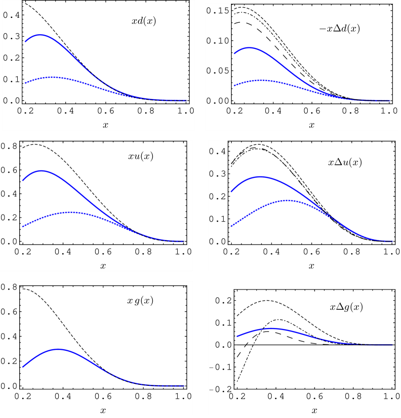
Figure 1: Quark and gluon parton distributions. The black curves correspond to the existing parametrizations: GRV Gluck:1998xa (short dashes), DSSV deFlorian:2009vb (long dashes) and LSS’10 Leader:2010rb (dash-dotted) at the scale $\mu^{2}=1GeV^{2}$ Cafarella:2003jr . The solid blue curve is our model prediction taking into account the contributions of the valence three-quark state and the state involving one additional gluon. The contribution of the valence state alone is shown by dots for comparison.

The unpolarized distributions are only sensitive to the total probability to find an extra gluon. We choose

$$P_{3qg}=P_{3qg^{\uparrow}}+P_{3qg^{\downarrow}}=0.33\,.$$ (78)

For the central values of the QCD sum rule estimates for the wave functions at the origin, Eq. (46), this value can be obtained assuming that the quark-gluon state is slightly more compact in transverse space as compared to the valence three-quark configuration:

$$a_{g}=a_{g}^{\uparrow}=a_{g}^{\downarrow}=0.9\,a_{3}\,,$$ (79)

which is reasonable.

The ratio $\Delta g(x)/g(x)$ is determined in our simple model by the ratio of the probabilities to find a gluon with helicity aligned an anti-aligned with that of the proton. In the rest of this work we take

$$\frac{P_{uudg^{\downarrow}}}{P_{uudg^{\uparrow}}}=\frac{2}{3}\frac{(\lambda_{1}^{g})^{2}}{(\lambda_{2}^{g})^{2}+(\lambda_{3}^{g})^{2}}=0.6\,\,(0.8\pm 0.2)$$ (80)

where the number in parenthesis is the QCD sum rule prediction, Eq. (46). The polarized quark distributions $\Delta u(x)$ and $\Delta d(x)$ also involve another ratio of the couplings, cf. Eq. (76), which is, however, small according to our estimates. The corresponding contributions to $\Delta u(x)$ and $\Delta d(x)$ are below 5%.

The results for the transversity distributions $\delta u(x)$, $\delta d(x)$ are shown in Fig. 2. These distributions are only very weakly constrained by the experiment, see e.g. the discussion in Refs. Anselmino:2007fs ; Anselmino:2007zr ; Anselmino:2008sj . Our results are generally similar to the other existing model predictions, see Ref. Barone:2001sp for a review and the corresponding references.

We remind that in this work we try to keep the model as simple as possible, restricting ourselves to contributions of the states with total zero angular momentum and the simplest, asymptotic shape of the four-particle quark-gluon proton distribution amplitude. It is seen that this simple approximation captures main features of parton distributions at large $x$ surprisingly well, although more sophisticated models are certainly needed for a quantitative description.

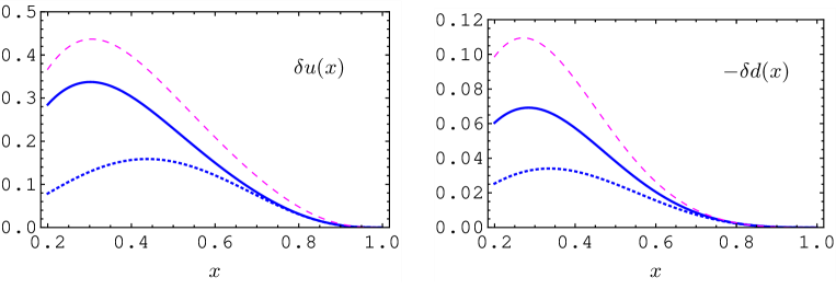
Figure 2: The quark transversity distribution $\delta q(x)$. The solid blue curve is our model prediction taking into account the contributions of the valence three-quark state and the state involving one additional gluon. The contribution of the valence state alone is shown by dots for comparison. The Soffer bound (77) is indicated by the (magenta) dashed curve.

V Twist-3 observables

V.1 Quark-antiquark-gluon correlation functions

A description of twist-three observables in the framework of collinear factorization involves quark-antiquark-gluon correlation functions which are defined as matrix elements of nonlocal (light-ray) three-particle operators. In the literature there exists apparently no “standard” definition of such operators, and also no standard notation. One of the usual choices Braun:2000yi is to consider the operators

$$\mathbb{S}^{\pm}_{\mu}(z_{1},z_{2},z_{3})=\frac{1}{2}\bar{q}(z_{1})\big{[}i\widetilde{F}_{\mu+}(z_{2})\pm F_{\mu+}(z_{2})\gamma_{5}\big{]}\gamma_{+}q(z_{3})\,$$ (81)

and define the twist-three correlations functions $D^{\pm}_{q}$ as the matrix elements

$$\langle{p,s|S^{\pm}_{\mu}(z_{1},z_{2},z_{3})|p,s}\rangle = 4m_{N}i(pn)[s_{\mu}(pn)-p_{\mu}(sn)]$$ (82)

$${}\times\int\mathcal{D}x\,e^{ipn\sum z_{i}x_{i}}D^{\pm}_{q}(x_{i})\,,$$

where $s_{\mu}$ is the proton spin vector which we assume to be normalized as $s^{2}=-1$. This formulation is often used e.g. in the studies of the nucleon structure function $g_{2}(x,Q^{2})$.

Here and below the integration measure $\mathcal{D}x$ is defined as

$$\int\mathcal{D}x=\int dx_{1}dx_{2}dx_{3}\,\delta(\sum x_{i})\,.$$ (83)

The difference to $[dx]_{3}$ (III.1) is that the momentum fractions sum up to zero.

A subtlety in using this definition is that the twist-three and twist-four contributions in $\mathbb{S}^{\pm}_{\mu}$ are not separated on the operator level. It can be more convenient to forgo the explicit Lorentz covariance and restrict oneself to transverse spin polarizations $(s_{T}\cdot n)=0$ introducing another set of operators Braun:2009mi :

$$\mathfrak{S}^{\pm}(z)=2is_{T}^{\mu}[\mathbb{S}^{+}_{\mu}(z_{1},z_{2},z_{3})\pm\mathbb{S}^{-}_{\mu}(z_{3},z_{2},z_{1})]\,.$$ (84)

The operators $\mathfrak{S}^{\pm}(z)$ are even (odd) with respect to the charge conjugation. One can show that Braun:2009mi

$$\left(\mathfrak{S}^{\pm}({z})\right)^{\dagger}=\pm\mathfrak{S}^{\pm}({z})$$

so that the $C$-even (“plus”) and $C$-odd (“minus”) $\mathfrak{S}$-operators are hermitian and antihermitian, respectively.

The corresponding matrix elements define the $C$-even and the $C$-odd twist-three correlations functions

$$\langle{p,s_{T}|\mathfrak{S}^{\pm}({z})|p,s_{T}}\rangle=2(pn)^{2}\int\mathcal{D}x\,e^{-i(pn)\sum_{k}x_{k}z_{k}}\,\mathfrak{S}^{\pm}({x})\,,$$ (85)

which are related to the $D^{\pm}$–functions introduced above as

$$8m_{N}D^{+}(x_{1},x_{2},x_{3}) = \mathfrak{S}^{+}(x_{1},x_{2},x_{3})-\mathfrak{S}^{-}(x_{1},x_{2},x_{3})\,,$$

$$8m_{N}D^{-}(x_{1},x_{2},x_{3}) = \mathfrak{S}^{+}(x_{3},x_{2},x_{1})+\mathfrak{S}^{-}(x_{3},x_{2},x_{1})\,.$$

Note that we use the same notation $\mathfrak{S}^{\pm}$ for the operators and the matrix elements, which hopefully will not lead to a confusion.

The helicity structure of the twist-three correlation functions can be made explicit going over to the two-component spinor notation. One obtains

$$\mathfrak{S}^{\pm}({z})=-{ig}\Big{[}\bar{s}\,\mathcal{Q}^{\pm}({z})-s\,\widetilde{\mathcal{Q}}^{\pm}({z})\Big{]}\,,$$ (87)

where $s=s^{1}+is^{2}$, $\bar{s}=s^{1}-is^{2}$, and

$$\mathcal{Q}^{\pm}({z}) =\! \bar{q}^{\downarrow}_{+}(z_{1})f_{++}(z_{2})q^{\downarrow}_{+}(z_{3})\pm\bar{q}^{\uparrow}_{+}(z_{3})f_{++}(z_{2})q^{\uparrow}_{+}(z_{1})\,,$$

$$\widetilde{\mathcal{Q}}^{\pm}({z}) =\! \bar{q}^{\uparrow}_{+}(z_{1})\bar{f}_{++}(z_{2})q^{\uparrow}_{+}(z_{3})\pm\bar{q}^{\downarrow}_{+}(z_{3})\bar{f}_{++}(z_{2})q^{\downarrow}_{+}(z_{1})\,.$$

The nucleon state with a transverse polarization can be expressed in terms of the helicity states $|{p,\pm}\rangle$ as

$$|{p,s_{T}}\rangle=\frac{1}{\sqrt{2}}\Big{[}|{p,+}\rangle+s\,|{p,-}\rangle\Big{]}.$$

Taking into account that the operators $\mathcal{Q}^{\pm}({z})$ increase and $\widetilde{\mathcal{Q}}^{\pm}({z})$ decrease helicity, it follows that

$$\langle{p,s_{T}|\mathfrak{S}^{\pm}({z})|p,s_{T}}\rangle=$$ (89)

$$= {ig}\Big{[}\langle{p,+|\mathcal{Q}^{\pm}(z)|p,-}\rangle-\langle{p,-|\widetilde{\mathcal{Q}}^{\pm}(z)|p,+}\rangle\Big{]}\,.$$

It is easy to see that $\widetilde{\mathcal{Q}}^{\pm}({z})=\pm[\mathcal{Q}^{\pm}({z})]^{\dagger}$, so that the two matrix elements on the r.h.s. of Eq. (89) are related and one does not need to consider the operators with a “tilde” explicitly.

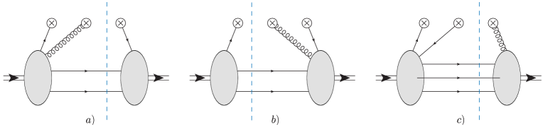
Figure 3: Twist-three correlation functions from the overlap of light-cone wave functions.

We define the distributions $\mathcal{Q}^{\pm}(x)$ as

$$\langle{p,+|\mathcal{Q}^{\pm}(z)|p,-}\rangle=-2i(pn)^{2}\int\mathcal{D}x\,e^{-i(pn)\sum x_{k}z_{k}}\mathcal{Q}^{\pm}(x)\,.$$ (90)

The $P$-parity implies (cf. Braun:2009mi )

$$\bigl{(}\mathcal{Q}^{\pm}(-x)\bigr{)}^{*}=\pm\mathcal{Q}^{\pm}(x)$$ (91)

and finally

$$\mathfrak{S}^{\pm}({x})=-g\,\mathcal{Q}^{\pm}(x)\,.$$ (92)

In the light-cone formalism, twist-three correlation functions are generated by the interference of Fock states with different particle content as illustrated in Fig. 3. The contributions shown schematically in Fig. 3a,b correspond to the interference of the three-quark and three-quark-gluon wave functions, whereas the one in Fig. 3c stands for the interference of the three-quark-gluon state with the one containing an extra quark-antiquark pair. The latter term contributes to a different kinematic region in momentum fractions compared to the first two terms and is missing to our accuracy.

Explicit expressions for the three-quark and three-quark-gluon Fock states for the nucleon with positive helicity are given in Sec. III. The corresponding states for the nucleon of negative helicity are given by the same expressions, Eqs. (III.1), (27), (31), where helicities of creation operators have to be flipped. The wave functions of the three-quark-gluon states of the nucleon with positive and negative helicity are the same, $[\Psi^{\uparrow\downarrow}_{1234}]_{(-)}=[\Psi^{\uparrow\downarrow}_{1234}]_{(+)}$, whereas for the valence three-quark state there is an overall sign difference: $[\Psi^{(0)}_{123}]_{(-)}=-[\Psi^{(0)}_{123}]_{(+)}$. All matrix elements in question can be expressed in terms of two correlation functions $\mathcal{Q}^{\uparrow(\downarrow)}_{q}(x)$ defined as

$${}_{uud}\langle{p,+|\bar{q}^{\uparrow}_{+}(z_{3})f_{++}(z_{2})q^{\uparrow}_{+}(z_{1})|p,-}\rangle_{uudg^{\uparrow}}$$

$$\hskip 56.9055pt=-2ip_{+}^{2}\int\mathcal{D}x\,e^{-ip_{+}\sum x_{i}z_{i}}\mathcal{Q}^{\uparrow}_{q}(x)\,,$$

$${}_{uud}\langle{p,+|\bar{q}^{\downarrow}_{+}(z_{1})f_{++}(z_{2})q^{\downarrow}_{+}(z_{3})|p,-}\rangle_{uudg^{\uparrow}}$$

$$\hskip 56.9055pt=-2ip_{+}^{2}\int\mathcal{D}x\,e^{-ip_{+}\sum x_{i}z_{i}}\mathcal{Q}^{\downarrow}_{q}(x)\,,$$ (93)

where the subscript $q=u,d$ stands for quark flavor. In particular

$$\mathcal{Q}_{q}^{\pm}(x)= \mathcal{Q}_{q}^{\downarrow}(x)\pm\mathcal{Q}_{q}^{\downarrow}(-x)+\mathcal{Q}_{q}^{\uparrow}(-x)\pm\mathcal{Q}_{q}^{\uparrow}(x)\,.$$ (94)

Using the ansatz for the LCWFs in Eqs. (23),(III.1) one can represent $\mathcal{Q}_{q}^{\uparrow(\downarrow)}(x)$ as convolution integrals of the distribution amplitudes. We obtain

$$\mathcal{Q}^{\downarrow}_{d}(x)= \frac{1}{2}A\theta(-x_{1},x_{2},x_{3})\frac{1}{x_{1}}\int\frac{d\xi_{1}}{\xi_{1}}\frac{d\xi_{2}}{\xi_{2}}\delta(1+x_{1}-\xi_{1}-\xi_{2})\Big{[}\phi(\xi_{1},-x_{1},\xi_{2})+\phi(\xi_{2},-x_{1},\xi_{1})\Big{]}\psi_{g}(\xi_{1},x_{3},\xi_{2},x_{2})\,,$$

$$\mathcal{Q}^{\downarrow}_{u}(x)= \frac{1}{2}A\theta(-x_{1},x_{2},x_{3})\frac{1}{x_{1}}\int\frac{d\xi_{1}}{\xi_{1}}\frac{d\xi_{2}}{\xi_{2}}\delta(1+x_{1}-\xi_{1}-\xi_{2})\phi(\xi_{1},-x_{1},\xi_{2})\Big{[}\psi^{(1)}_{g}(\xi_{1},x_{3},\xi_{2},x_{2})-\psi^{(2)}_{g}(\xi_{1},\xi_{2},x_{3},x_{2})\Big{]},$$

$$\mathcal{Q}^{\uparrow}_{d}(x)= A\theta(x_{1},x_{2},-x_{3})\frac{1}{x_{3}}\int\frac{d\xi_{1}}{\xi_{1}}\frac{d\xi_{2}}{\xi_{2}}\delta(1+x_{3}-\xi_{1}-\xi_{2})\phi(\xi_{1},\xi_{2},-x_{3})\left[\frac{1}{2}\psi^{(1)}_{g}(\xi_{1},\xi_{2},x_{1},x_{2})+\psi^{(2)}_{g}(\xi_{1},x_{1},\xi_{2},x_{2})\right],$$

$$\mathcal{Q}^{\uparrow}_{u}(x)= -A\theta(x_{1},x_{2},-x_{3})\frac{1}{x_{3}}\int\frac{d\xi_{1}}{\xi_{1}}\frac{d\xi_{2}}{\xi_{2}}\delta(1+x_{3}-\xi_{1}-\xi_{2})\Big{\{}\phi(-x_{3},\xi_{1},\xi_{2})\left[\psi^{(1)}_{g}(x_{1},\xi_{1},\xi_{2},x_{2})+\frac{1}{2}\psi^{(2)}_{g}(x_{1},\xi_{2},\xi_{1},x_{2})\right]$$

$$+\Big{[}\phi(-x_{3},\xi_{2},\xi_{1})+\phi(\xi_{1},\xi_{2},-x_{3})\Big{]}\Big{[}\psi_{g}(x_{1},\xi_{2},\xi_{1},x_{2})-\frac{1}{2}\psi_{g}(\xi_{1},\xi_{2},x_{1},x_{2})\Big{]}\Big{\}},$$ (95)

where it is implicitly assumed that $x_{1}+x_{2}+x_{3}=0$, the Heaviside step-function with several arguments is defined as $\theta(a,b,c)\equiv\theta(a)\theta(b)\theta(c)$, and

$$A=\frac{1}{3}(4\pi)^{4}\left(\frac{a_{3}^{2}a_{g}^{2}}{a_{3}^{2}+a_{g}^{2}}\right)^{2}.$$ (96)

The distribution $\psi_{g}$ is defined in Eq. (58). The QCD sum rule result $\lambda_{3}^{g}\ll\lambda_{1,2}^{g}$ (46) implies that $\psi_{g}^{(1)}\simeq\psi_{g}^{(2)}$ and as a consequence both helicity down functions $\mathcal{Q}_{u,d}^{\downarrow}(x)$ are suppressed in comparison with the helicity up functions $\mathcal{Q}_{u,d}^{\uparrow}(x)$.

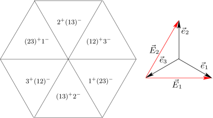
Figure 4: Support properties of twist-three correlation functions in barycentric coordinates. For the explanation of different regions see text.

Note that we use a symmetric notation with quark, antiquark and gluon momentum fractions are treated equally so that the momentum conservation condition is $x_{1}+x_{2}+x_{3}=0$. Support properties of the correlation functions Jaffe:1983hp can most easily be shown going over to barycentric coordinates Braun:2009mi as shown in Fig. 4:

$$\vec{x}=x_{1}\vec{e}_{1}+x_{2}\vec{e}_{2}+x_{3}\vec{e}_{3}=x_{1}\vec{E}_{1}+x_{2}\vec{E}_{2}\,.$$

Three-parton correlation functions, in general, “live” inside a hexagon-shaped area which can further be decomposed in six different regions (triangles). The triangles labeled $(12)^{+}3^{-}$, $2^{+}(13)^{-}$, etc., correspond to different subprocesses at the parton level Jaffe:1983hp ; For each parton $k=1,2,3$  “plus” stays for emission ($x_{k}>0$) and “minus” for absorption ($x_{k}<0$). Alternatively, one may think of “plus” and “minus” labels as indicating whether the corresponding parton appears in the direct or the final amplitude in the cut diagram, cf. Fig. 3. It is important that different regions do not have autonomous scale dependence; they “talk” to each other and get mixed under the evolution, see Ref. Braun:2009mi for a detailed discussion.

Our model predictions for the correlation functions $\mathcal{Q}_{d}^{+}(x)$ and $-\mathcal{Q}_{u}^{+}(x)$ (note opposite sign), Eq. (90), are shown in Fig. 6 and Fig. 6, respectively. Both distributions are symmetric with respect to the center of the hexagon: $\mathcal{Q}_{q}^{+}(x_{1},x_{2},x_{3})=\mathcal{Q}_{q}^{+}(-x_{1},-x_{2},-x_{3})$, which is a consequence of $P$-parity, cf. Eq. (91). Each of the four terms $\mathcal{Q}_{q}^{\uparrow(\downarrow)}(\pm x)$ in Eq. (94) is confined to a different “triangle” and, hence, has a different partonic interpretation:

$$\mathcal{Q}_{q}^{\uparrow}(x)\,:\,(12)^{+}3^{-}, \mathcal{Q}_{q}^{\uparrow}(-x)\,:\,3^{+}(12)^{-},$$

$$\mathcal{Q}_{q}^{\downarrow}(x)\,:\,(23)^{+}1^{-}, \mathcal{Q}_{q}^{\downarrow}(-x)\,:\,1^{+}(23)^{-}.$$ (97)

The larger contributions, e.g. in the $(12)^{+}3^{-}$ region, correspond to (valence) quark emission with momentum fraction $x_{1}>0$ and subsequent absorption with momentum fraction $-x_{3}>x_{1}>0$, accompanied with gluon emission with momentum fraction $x_{2}>0$. The smaller contributions, e.g. in the $1^{+}(23)^{-}$ region, differ from the above in that the gluon with momentum fraction $-x_{2}>0$ is absorbed and thus $x_{1}>-x_{3}>0$. Note that there is no symmetry between gluon emission and absorption, which may be somewhat counterintuitive.

The dominant, gluon emission contribution to the $\bar{u}Gu$ correlation function $\mathcal{Q}_{u}^{\uparrow}(x)$ is roughly factor two larger compared to the $\bar{d}Gd$ distribution, $\mathcal{Q}_{d}^{\uparrow}(x)$, and has the opposite sign. The contributions of gluon absorption, $\mathcal{Q}_{u}^{\downarrow}(x)$ and $\mathcal{Q}_{d}^{\downarrow}(x)$, have the same sign for $u$- and $d$-quarks, and are much smaller compared to gluon emission.

Our model correlation functions vanish in the $2^{+}(13)^{-}$ and $(13)^{+}2^{-}$ regions. This property is an artefact of neglecting contributions of the type shown in Fig. 3c which are formally higher order in the Fock expansion. These contributions can be estimated using a model for the five-parton $qqq(\bar{q}q)$ state from Ref. Diehl:1998kh and turn out to be considerably smaller than the ones considered here.

The “minus” correlation functions $\mathcal{Q}_{u}^{-}(x)$ and $\mathcal{Q}_{d}^{-}(x)$ are obtained from the “plus” ones by changing the sign of the contributions in the $(12)^{+}3^{-}$ and $1^{+}(23)^{-}$ regions, so we do not show them separately.

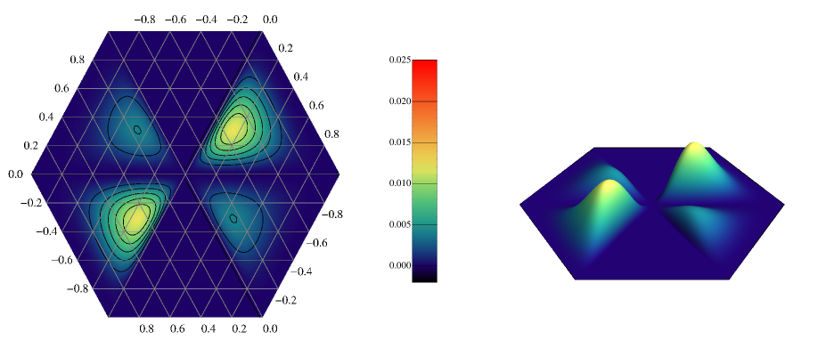
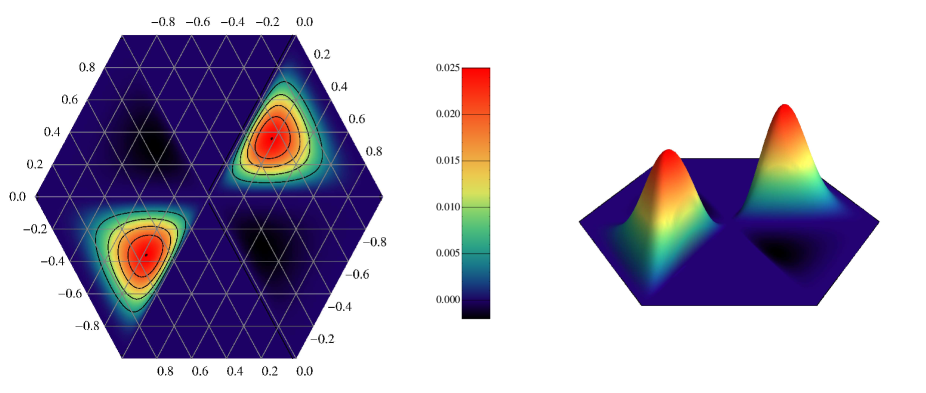
Figure 5: The quark-antiquark-gluon twist-three correlation function $\mathcal{Q}_{d}^{+}(x)$ at the reference scale 1 GeV.

Figure 6: The quark-antiquark-gluon twist-three correlation function $-\mathcal{Q}_{u}^{+}(x)$ at the reference scale 1 GeV.

V.2 The structure function $g_{2}(x,Q^{2})$

The structure function $g_{2}(x_{B},Q^{2})$ is given by the sum of the Wandzura-Wilczek (WW) and genuine twist-3 contributions

$$g_{2}(x_{B},Q^{2})=g^{WW}_{2}(x_{B},Q^{2})+g^{tw-3}_{2}(x_{B},Q^{2})\,.$$ (98)

The WW contribution reads

$$g^{WW}_{2}(x_{B},Q^{2})=-g_{1}(x_{B},Q^{2})+\int_{x_{B}}^{1}\frac{dy}{y}g_{1}(y,Q^{2})\,,$$ (99)

where

$$g_{1}(x_{B},Q^{2})=\frac{1}{2}\sum_{q}e_{q}^{2}\left[\Delta q(x_{B},Q^{2})+\Delta q(-x_{B},Q^{2})\right]\,.$$ (100)

The twist-3 contribution $g^{tw-3}_{2}(x_{B},Q^{2})$ can be written as

$$g^{tw-3}_{2}(x_{B},Q^{2})=$$ (101)

$$= \frac{1}{2}\sum_{q}e_{q}^{2}\int_{x_{B}}^{1}\frac{d\xi}{\xi}\Big{[}\Delta q_{T}(\xi,Q^{2})+\Delta q_{T}(-\xi,Q^{2})\Big{]}\,,$$

where $\Delta q_{T}(\xi)$ is defined in terms of the $D^{+}$–function introduced in Eq. (82):

$$\Delta q_{T}(\xi)=4\int\mathcal{D}x\,D_{q}^{+}(x)\frac{d}{dx_{3}}\left[\frac{\delta(\xi+x_{3})-\delta(\xi-x_{1})}{x_{1}+x_{3}}\right]\,.$$ (102)

As above, the subscript $q$ refers to the contribution of a given quark flavor. In terms of the $\mathcal{Q}_{q}^{\uparrow(\downarrow)}(x)$–functions one obtains

$$D_{q}^{+}(x)= -\frac{g}{4m_{N}}\left[\mathcal{Q}_{q}^{\uparrow}(x)+\mathcal{Q}_{q}^{\downarrow}(-x)\right].$$ (103)

To avoid confusion, in this section we use the notation $x_{B}$ for the Bjorken variable, whereas $x$ is reserved for the set of parton momentum fractions $x=\{x_{1},x_{2},x_{3}\}$.

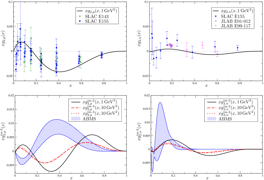
Figure 7: Upper panels: Experimental results on the proton (left) and neutron (right) structure function $g_{2}(x_{B},Q^{2})$ compared to our model calculation at the scale $Q^{2}=1$ GeV². Lower panels: The twist-three contributions $xg^{twist-3}_{2}(x_{B},Q^{2})$ for the proton (left) and neutron (right) compared to the analysis in Ref. Accardi:2009au (shaded areas). Our model predictions at the scale $Q^{2}=1$ GeV² and $Q^{2}=10$ GeV² are shown by the black solid and dashed red curves, respectively. The predictions at $10$ GeV² obtained using an approximate evolution equation from Refs. Ali:1991em ; Braun:2001qx are shown by the red dotted curves for comparison.

Under a plausible assumption that the spin-dependent part of the forward Compton amplitude satisfies a dispersion relation without subtractions, the integral of $g_{2}(x_{B},Q^{2})$ and, hence, of $g^{tw-3}_{2}(x_{B},Q^{2})$ vanishes Burkhardt:1970ti

$$\int_{0}^{1}dx_{B}\,g^{tw-3}_{2}(x_{B},Q^{2})=0\,.$$ (104)

This statement is known as the Burkhardt-Cottingham (BC) sum rule.

Using Eqs. (V.1) one finds that in our model $D_{q}^{+}(x)$ is nonzero only when $x_{1}\geq 0$ and $x_{3}\leq 0$. This, in turn, implies that $\Delta q_{T}(\xi)$ vanishes for $\xi<0$ (i.e. there is no antiquark contribution). As a consequence, in our model $g^{tw-3}_{2}(x_{B},Q^{2})$ satisfies in addition to Burkhardt-Cottingham (104) also the Efremov-Leader-Teryaev (ELT) sum rule Efremov:1996hd :

$$\int_{0}^{1}dx_{B}\,x_{B}\,g^{tw-3}_{2}(x_{B},Q^{2})=0\,.$$ (105)

For the second moments one obtains

$$d_{2,p} = 3\int_{0}^{1}dx_{B}\,x_{B}^{2}g_{2,p}^{tw-3}(x_{B})$$

$$= \frac{5}{32}Af_{N}\Big{[}\lambda_{2}^{g}\left(1+\frac{5a+b}{12}\right)+\lambda_{3}^{g}\Big{(}1+\frac{a+5b}{12}\Big{)}\Big{]},$$

$$d_{2,n} = 3\int_{0}^{1}dx_{B}\,x_{B}^{2}g_{2,n}^{tw-3}(x_{B})$$

$$= -\frac{5}{32}Af_{N}\Big{[}\lambda_{2}^{g}\Big{(}1+\frac{b-5a}{12}\Big{)}+\lambda_{3}^{g}\Big{(}1+\frac{a-5b}{12}\Big{)}\Big{]}.$$

The corresponding numerical values are, at the scale 1 GeV:

$$d_{2,p} = \phantom{-}0.0016\,,\qquad d_{2,n}\,=\,-0.00072\,.$$ (107)

Both numbers compare very well to the lattice QCD Gockeler:2000ja , QCD sum rules Balitsky:1989jb ; Stein:1994zk and chiral quark soliton model Wakamatsu:2000ex calculations. The negative value of $d_{2}$ for the neutron (in all models) is in conflict, however, with the existing experimental average:

$$d^{\rm exp}_{2,p} = 0.0032\pm 0.0017~{}\text{\cite[cite]{\@@bibref{Authors Phrase1YearPhrase2}{Anthony:2002hy}{\@@citephrase{(}}{\@@citephrase{)}}}}\,,$$

$$d^{\rm exp}_{2,n} = 0.0062\pm 0.0028~{}\text{\cite[cite]{\@@bibref{Authors Phrase1YearPhrase2}{Zheng:2004ce}{\@@citephrase{(}}{\@@citephrase{)}}}}\,.$$ (108)

Further, a straightforward calculation gives

$$g^{tw-3}_{2,p}(x_{B}) = 0.0436772\Big{(}\ln x_{B}+\bar{x}_{B}+1/2\bar{x}_{B}^{2}\Big{)}$$

$${}+\bar{x}_{B}^{3}\Big{(}1.57357-5.94918\bar{x}_{B}+6.74412\bar{x}_{B}^{2}-2.19114\bar{x}_{B}^{3}\Big{)},$$

$$g^{tw-3}_{2,n}(x_{B}) = 0.0655158\Big{(}\ln x_{B}+\bar{x}_{B}+1/2\bar{x}_{B}^{2}\Big{)}$$

$${}+\bar{x}_{B}^{3}\Big{(}0.130996-1.12101\bar{x}_{B}+2.31342\bar{x}_{B}^{2}-1.20598\bar{x}_{B}^{3}\Big{)}$$

(at the reference scale 1 GeV) for the proton and neutron, respectively.

Our results for the full structure function $g_{2}(x_{B},Q^{2})$ are compared to the experimental data Abe:1998wq ; Zheng:2004ce ; Kramer:2005qe in Fig. 7 (upper panels) and, separately, for the twist-three contribution $g_{2}^{tw-3}(x_{B})$ to the analysis in Ref. Accardi:2009au (lower panels). The twist-three contributions are shown at the model scale $Q^{2}=1$ GeV² and after the evolution to a higher scale $Q^{2}=10$ GeV². The scale dependence was calculated in two ways: using exact (one-loop) evolution equations for the relevant quark-antiquark-gluon correlation functions from Ref. Braun:2009mi (dashed curves), and using the much simpler evolution equation from Refs. Ali:1991em ; Braun:2001qx which is based on the large-$N_{c}$ and large-$x_{B}$ approximation and only involves the $g_{2}^{tw-3}(x_{B})$ structure function itself (dotted curves). Since we are interested primarily in the large $x_{B}$ region, we used flavor-nonsinglet evolution equations which are simpler. The results of both approaches almost coincide within the line thickness. A good accuracy of this approximation was expected but has never been checked in a dynamical model calculation. Note that effects of the evolution are generally significant because of large anomalous dimensions of twist-three operators, and have to be taken into account in the analysis of the experimental data.

As seen from Fig. 7, the twist-three contribution to the structure function $g_{2}(x_{B},Q^{2})$ at large $x_{B}$ proves to be positive for the proton and negative for the neutron. This prediction can be traced to the relative signs of the three-quark-gluon couplings and is largely model-independent. It is in agreement with Ref. Accardi:2009au . In the intermediate region $0.2<x_{B}<0.5$ the twist-three contribution $g_{2,p}^{tw-3}(x_{B})$ changes sign and becomes negative in our calculation, whereas it remains positive according to the data analysis in Ref. Accardi:2009au . This difference may well be due to contributions of higher Fock states, with two or more gluons, and probably also partially remedied by using a more sophisticated model for the three-quark-gluon wave function. A detailed analysis would be interesting but goes beyond the tasks of this paper. Another issue is that in Accardi:2009au the ELT sum rule is strongly violated, which suggests the existence of a large positive flavor-singlet contribution at $x_{B}\sim 0.1$ due to gluons or sea quark-antiquark pairs. Such contributions are related to the twist-three three-gluon correlation functions and are missing in our present framework.

V.3 Single spin asymmetries

The quark-antiquark-gluon correlation functions considered in this work are precisely those responsible for transverse single spin asymmetries (SSA) observed in different hadronic reactions, if described in the framework of collinear factorization Efremov:1981sh ; Efremov:1984ip ; Qiu:1991pp ; Qiu:1991wg ; Efremov:1994dg ; Qiu:1998ia ; Kanazawa:2000hz ; Kanazawa:2000cx ; Eguchi:2006mc ; Koike:2007rq ; Kang:2008ih . The distributions $T_{\bar{q}Fq}({x})$, $\Delta T_{\bar{q}Fq}({x})$ introduced in this context in Ref. Braun:2009mi are expressed in terms of $\mathcal{Q}_{q}^{\uparrow(\downarrow)}$–functions as follows:

$$T_{\bar{q}Fq}({x_{1},x_{2},x_{3}})=$$

$$= \frac{1}{4}\Big{[}(1\!+\!\mathcal{P}_{13})\mathfrak{S}^{+}({x})+(1\!-\!\mathcal{P}_{13})\mathfrak{S}^{-}({x})\Big{]}$$

$$= -\frac{g}{2}\Big{[}\mathcal{Q}_{q}^{\uparrow}(x_{3},x_{2},x_{1})+\mathcal{Q}_{q}^{\uparrow}(-x_{1},-x_{2},-x_{3})$$

$${}+\mathcal{Q}_{q}^{\downarrow}(x_{1},x_{2},x_{3})+\mathcal{Q}_{q}^{\downarrow}(-x_{3},-x_{2},-x_{1})\Big{]}\,,$$

$$\Delta T_{\bar{q}Fq}({x_{1},x_{2},x_{3}})=$$ (110)

$$= -\frac{1}{4}\Big{[}(1\!-\!\mathcal{P}_{13})\mathfrak{S}^{+}({x})+(1\!+\!\mathcal{P}_{13})\mathfrak{S}^{-}({x})\Big{]}$$

$$= -\frac{g}{2}\Big{[}\mathcal{Q}_{q}^{\uparrow}(x_{3},x_{2},x_{1})-\mathcal{Q}_{q}^{\uparrow}(-x_{1},-x_{2},-x_{3})$$

$${}-\mathcal{Q}_{q}^{\downarrow}(x_{1},x_{2},x_{3})+\mathcal{Q}_{q}^{\downarrow}(-x_{3},-x_{2},-x_{1})\Big{]}\,.$$

A common notation Kang:2008ey is to show quark momenta only:

$${\mathcal{T}}_{q,F}(x,x^{\prime}) \equiv T_{\bar{q}Fq}(-x^{\prime},x^{\prime}-x,x)\,,$$

$${\mathcal{T}}_{\Delta q,F}(x,x^{\prime}) \equiv \Delta T_{\bar{q}Fq}(-x^{\prime},x^{\prime}-x,x)\,,$$ (111)

Written in this way, the distributions are symmetric (antisymmetric) functions of the arguments: ${\mathcal{T}}_{q,F}(x,x^{\prime})={\mathcal{T}}_{q,F}(x^{\prime},x)$ and $\Delta{\mathcal{T}}_{q,F}(x,x^{\prime})=-\Delta{\mathcal{T}}_{q,F}(x^{\prime},x)$. A yet another notation for the same functions in a different normalization is used in the recent analysis in Ref. Kanazawa:2010au :

$$G_{F}^{q}(x,x^{\prime}) \equiv -\frac{2}{m_{N}}T_{\bar{q}Fq}(-x^{\prime},x^{\prime}-x,x)\,,$$

$$\widetilde{G}_{F}^{q}(x,x^{\prime}) \equiv \frac{2}{m_{N}}\Delta T_{\bar{q}Fq}(-x^{\prime},x^{\prime}-x,x)\,.$$ (112)

Figure 8: The quark-antiquark-gluon twist-three correlation function $-T_{\bar{d}Fd}(x)$ at the reference scale $\mu^{2}=1$ GeV² (left) and $\mu^{2}=10$ GeV² (right).

In the framework of collinear factorization, SSAs originate from imaginary (pole) parts of propagators in the hard coefficient functions. In the leading order, taking a pole part enforces vanishing of one of the momentum fractions in the twist-3 parton distribution, and are classified as soft gluon pole (SGP) or soft fermion pole (SFP), depending on which momentum is put to zero, respectively. Such “pole” contributions are therefore considered to be main source of the observed asymmetries and can be estimated from the available experimental data Kouvaris:2006zy ; Kanazawa:2010au .

Since our approximation for the nucleon wave function does not contain antiquarks, the $T_{\bar{q}Fq}$, $\Delta T_{\bar{q}Fq}$ distributions are nonzero in the $(23)^{+}1^{-}$ and $(12)^{-}3^{+}$ regions only, cf. Fig. 4. Moreover, both distributions vanish at the boundaries of parton regions where one of the momentum fractions goes to zero, and, hence, both SGP and SFP terms vanish as well. This property is an obvious artefact of the truncation of the Fock expansion to a few lowest components: The LCWF of each Fock state vanishes whenever momentum fraction of any parton goes to zero and the same property holds true for the correlation functions. Our model for the gluon distribution $xg(x)$ in Fig. 1 vanishes at $x\to 0$ for the very same reason.

For the leading-twist parton distributions, a possible way out is to assume the valence-type input at a certain low scale, and construct realistic dynamical models by applying QCD evolution equations that include multiple soft gluon radiation. This approach was suggested by Glück, Reya and Vogt (GRV) Gluck:1994uf ; Gluck:1998xa and proved to be very successful phenomenologically. Exploiting the same idea for the twist-three distributions suggests itself.

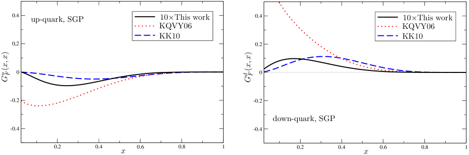
Figure 9: Radiatively generated SGP distributions $G_{F}^{q}(x,x)$ at $Q^{2}=10$ GeV² rescaled by factor 10, shown by the solid curves, as compared to the phenomenological studies of spin asymmetries in high transverse momentum meson production in $pp$ colisions Kouvaris:2006zy ; Kanazawa:2010au .

It is easy to see that both the SGP and SFP contributions reappear once QCD evolution is taken into account. The full one-loop evolution equation for the functions $T_{\bar{q}Fq}$, $\Delta T_{\bar{q}Fq}$ is rather cumbersome and can be found in Braun:2009mi . For our present purposes the flavor-nonsinglet evolution equation is sufficient. Restricting ourselves to the SGP kinematics $x_{2}\to 0$ one obtains, to the one-loop accuracy

$$\mathcal{T}_{q,F}(x,x;\mu^{2}) = \mathcal{T}_{q,F}(x,x;\mu_{0}^{2})+\frac{\alpha_{s}}{2\pi}\ln\frac{\mu^{2}}{\mu_{0}^{2}}\Big{\{}\int_{x}^{1}\frac{d\xi}{\xi}\Big{[}P_{qq}(z)\mathcal{T}_{q,F}(\xi,\xi)+\frac{N_{c}}{2}\frac{1+z}{1-z}\mathcal{T}_{q,F}(x,\xi)-\frac{N_{c}}{2}\frac{1+z^{2}}{1-z}\mathcal{T}_{q,F}(\xi,\xi)$$ (113)

$${}-\frac{N_{c}}{2}\mathcal{T}_{\Delta q,F}(x,\xi)+\frac{1}{2N_{c}}(1-2z)\mathcal{T}_{q,F}(x,x-\xi)-\frac{1}{2N_{c}}\mathcal{T}_{\Delta q,F}(x,x-\xi)\Big{]}-N_{c}\mathcal{T}_{q,F}(x,x)\Big{\}}^{\mu_{0}^{2}},$$

where it is assumed that $x>0$, $P_{qq}(z)$ is the usual Altarelli–Parisi splitting function and $z=x/\xi$. Even if $\mathcal{T}_{q,F}(x,x;\mu_{0}^{2})=0$, a non-zero SGP contribution is generated at a higher scale $\mu^{2}$. It is given by a certain integral of $T_{\bar{q}Fq}$, $\Delta T_{\bar{q}Fq}$ away from the line $x_{2}=0$, and involves large quark momentum fractions only, $\xi>x$. (For a detailed discussion of integration regions in Eq. (113) see Ref. Braun:2009mi .)

One difficulty in following the GRV approach is that the initial condition for the evolution has to be taken at a very low scale $\mu^{2}_{\rm GRV}\simeq 0.25$ GeV² Gluck:1994uf ; Gluck:1998xa whereas our model is formulated at $\mu^{2}_{0}=1$ GeV². The advantage of using the higher scale is that we have been able to use QCD perturbation theory and operator product expansion to get some insight in the structure of the lowest Fock states, but the price to pay is that the nucleon at the scale 1 GeV already contains significant admixture of yet higher states, with several gluons and quark-antiquark pairs, which we do not know much about. These additional contributions are not taken into account in this work, and this is the reason that we underestimate parton distributions at small $x$, cf. Fig. 1.

A consistent implementation of the GRV program would require to give up QCD motivated models for the $qqq$ and $qqqg$ states and resort to purely phenomenological parametrizations. We leave this study for future work. Instead, in what follows we show the results corresponding to the evolution of our model twist-three parton distribution from $1$ GeV² to an ad hoc scale $\mu^{2}=10$ GeV². This calculation should be considered as an illustration, since effects of the QCD evolution from the GRV scale $\mu^{2}_{\rm GRV}\simeq 0.25$ GeV² are, generally, much larger.

As an example, in Fig. 8 we show the the quark-antiquark-gluon twist-three correlation function $T_{\bar{d}Fd}(x)$ (with opposite sign) at the model scale $\mu^{2}=1$ GeV² (left) and after the evolution to $\mu^{2}=10$ GeV² (right). As already mentioned above, in our model (left picture) this correlation function is only nonzero in the two left-most triangle regions corresponding to emission and subsequent absorption of the (valence) quark. The upper and the lower triangles corresponds to gluon emission and absorption, respectively. The longest diagonals of the hexagon, connecting diametrically opposite vertices, correspond to vanishing of one of the parton momentum fractions. In particular, on the horizontal diagonal $x_{2}=0$, i.e. it corresponds to the SGP kinematics, and on the other two diagonals either $x_{1}=0$ or $x_{3}=0$, so they stand for the SFPs. The two triangles that come next to the right and include the upper (or the lower) edges of the hexagon, correspond to the contributions of the type shown in Fig. 3 where a gluon is emitted and a quark-antiquark pair is absorbed (or vice versa). These contributions are thus analogous to the so-called ERBL regions in off-forward parton distributions and, formally, are of higher order in the Fock expansion. Finally, the two right-most triangles correspond to the antiquark distributions.

Once the QCD evolution is taken into account, different parton regions get mixed. In particular the gap between the $x_{2}>0$ and $x_{2}<0$ regions gets closed and the SGP term appears, see Fig. 8 (right picture). The SFP terms are also generated, but remain very small because the corresponding terms in the evolution equations are $1/N_{C}$ suppressed.

The radiatively generated SGP distributions $G_{F}^{q}(x,x)$ at $Q^{2}=10$ GeV² are shown in Fig. 9 and compared there with the results of phenomenological studies of spin asymmetries in high transverse momentum meson production in $pp$ colisions Kouvaris:2006zy ; Kanazawa:2010au . Our distributions are of the same sign and similar shape compared to these studies, but about one order of magnitude smaller. It is plausible that much larger SGP contributions can be generated from the similar valence-like ansatz if the QCD evolution is started at a low scale of the order of $\mu^{2}_{\rm GRV}\simeq 0.25$ GeV² Gluck:1994uf ; Gluck:1998xa . The SFP contributions that we obtain in this exercise appear to be two orders of magnitude below the estimates in Ref. Kanazawa:2010au , albeit with the correct sign. It is unlikely that such large contributions can be obtained radiatively starting from the valence-like ansatz, unless one assumes the existence of antiquarks with large momentum fraction at low scales in the proton WF.

VI Conclusions

In this work we explored the possibility to construct higher-twist parton distributions in a nucleon at some low reference scale from convolution integrals of the light-cone wave functions.

To this end we have studied the general structure and introduced simple models for the four-particle nucleon LCWFs involving three valence quarks and a gluon with total orbital momentum zero, and estimated their normalization (WF at the origin) using QCD sum rules. We have shown that truncating the Fock expansion at this order, that is taking into account valence three-quark configuration and those with one additional gluon, provides one with a reasonable description of both polarized and unpolarized parton densities at large values of Bjorken variable $x\geq 0.5$.

Using this set of LCWFs, twist-three quark-antiquark-gluon parton distributions have been constructed as convolution integrals of $qqqg$ and valence three-quark components, which enter the description of many hard reactions in QCD in the framework of collinear factorization. In particular the twist-three contribution to the polarized structure function $g_{2}(x,Q^{2})$ is given by a certain integral of the three-particle distribution over the parton momentum fractions, and thus is a measure of its “global” properties. Our calculation correctly reproduces the sign and the order of magnitude of the twist-3 term at large $x$, without free parameters.

Transverse single spin asymmetries, on the other hand, are sensitive to “local” properties of the three-particle correlation functions in specific configurations where one of the momentum fractions vanishes. Since our approximation for the nucleon wave function only includes a few lowest Fock components, and since the LCWF of each Fock state vanishes whenever momentum fraction of any parton goes to zero, both “soft gluon pole” and “soft fermion pole” terms vanish at the scale where the model is formulated. They are, however, generated by QCD evolution that brings in multiple soft gluon emission. Our results suggest that realistic dynamical models of the the twist-three distributions (and the pole terms) can be obtained following the GRV-like approach on the level of WFs, i.e. assuming that the nucleon state at a very low scale can be described in terms of a few Fock components, including the valence quarks, one additional gluon and, probably, a quark-antiquark pair, and applying QCD evolution equations.

An obvious problem with this strategy is that the starting scale has to be chosen very low, of the order of $\mu^{2}_{\rm GRV}\simeq 0.25$ GeV² Gluck:1994uf ; Gluck:1998xa , and thus the modelling of the wave functions necessarily becomes purely phenomenological. In spite of this, and the usual criticism of the application of perturbative QCD evolution equations at very low scales, we believe that such an approach has good chances to provide us with some intuition on the structure of higher-twist parton distributions in general, which is currently not available. This work is in progress and the results will be published elsewhere.

Appendix A QCD sum rules for the quark-gluon wave functions at the origin

The definitions of quark-gluon twist-4 nucleon DAs (43) Braun:2008ia can be rewritten in conventional Dirac bispinor notation as follows:

$$ig\epsilon^{ijk}\langle 0|\Big{[}u^{i}_{\downarrow}(z_{1})C\not{n}u^{j}_{\uparrow}(z_{2})\Big{]}\gamma^{\nu}\not{n}d^{l}_{\downarrow}(z_{3})F_{n\nu}^{kl}(z_{4})|p\rangle = \frac{1}{4}m_{N}p_{+}^{2}\not{n}N^{\uparrow}(p)\int[dx]_{3}\,e^{-ip_{+}\sum x_{i}z_{i}}\Phi_{4}^{g}(x),$$

$$ig\epsilon^{ijk}\langle 0|\Big{[}u^{i}_{\uparrow}(z_{1})C\not{n}u^{l}_{\downarrow}(z_{2})\Big{]}\gamma^{\nu}\not{n}d^{k}_{\downarrow}(z_{3})F_{n\nu}^{jl}(z_{4})|p\rangle = \frac{1}{4}m_{N}p_{+}^{2}\not{n}N^{\uparrow}(p)\int[dx]_{3}\,e^{-ip_{+}\sum x_{i}z_{i}}\Psi_{4}^{g}(x),$$

$$ig\epsilon^{ijk}\langle 0|\Big{[}u^{i}_{\downarrow}(z_{1})C\gamma_{\nu}\not{n}d^{j}_{\downarrow}(z_{2})\Big{]}\not{n}u^{l}_{\downarrow}(z_{3})F_{n\nu}^{kl}(z_{4})|p\rangle = \frac{1}{4}m_{N}p_{+}^{2}\not{n}N^{\uparrow}(p)\int[dx]_{3}\,e^{-ip_{+}\sum x_{i}z_{i}}\Xi_{4}^{g}(x),$$ (A.114)

where $F_{n\nu}^{kl}\equiv n^{\mu}F^{a}_{\mu\nu}(t^{a})_{kl}$. The normalization of the DAs is determined by the matrix elements of the corresponding local operators. In what follows we estimate these matrix elements using the classical SVZ QCD sum rule approach Shifman:1978bx .

To this end we define isospin-1/2 twist-4 quark-gluon operators:

$$\eta_{1}^{g}(x) = \frac{2}{3}ig\epsilon^{ijk}\Big{[}\Big{(}u^{i}(x)C\not{n}u^{j}(x)\Big{)}\gamma^{\nu}\not{n}d^{l}(x)-\Big{(}u^{i}(x)C\not{n}d^{j}(x)\Big{)}\gamma^{\nu}\not{n}u^{l}(x)\Big{]}F_{n\nu}^{kl}(x)\,,$$

$$\eta_{2}^{g}(x) = \frac{2}{3}ig\epsilon^{ijk}\Big{[}\Big{(}u^{i}(x)C\gamma_{5}\not{n}u^{l}(x)\Big{)}\gamma^{\nu}\not{n}d^{k}(x)-\Big{(}u^{i}(x)C\gamma_{5}\not{n}d^{l}(x)\Big{)}\gamma^{\nu}\not{n}u^{k}(x)\Big{]}F_{n\nu}^{jl}(x)\,,$$

$$\eta_{3}^{g}(x) = \frac{2}{3}ig\epsilon^{ijk}\Big{[}\Big{(}u^{i}(x)C\gamma^{\nu}\not{n}u^{j}(x)\Big{)}\not{n}d^{l}(x)-\Big{(}u^{i}(x)C\gamma^{\nu}\not{n}d^{j}(x)\Big{)}\not{n}u^{l}(x)\Big{]}F_{n\nu}^{kl}(x).$$ (A.115)

Matrix elements of these operators sandwiched between vacuum and the proton state are related to the couplings introduced in Eq. (46):

$$\langle 0|\eta_{1}^{g}(0)|p\rangle = -\frac{1}{4}\Big{(}\lambda_{2}^{g}-\frac{1}{3}\lambda_{3}^{g}\Big{)}\,m_{N}p_{+}^{2}\not{n}\gamma_{5}N(p)\,,$$

$$\langle 0|\eta_{2}^{g}(0)|p\rangle = \phantom{-}\frac{1}{6}\Big{(}\lambda_{2}^{g}+\lambda_{3}^{g}\Big{)}m_{N}p_{+}^{2}\not{n}N(p)\,,$$

$$\langle 0|\eta_{3}^{g}(0)|p\rangle = \phantom{-}\frac{1}{6}\Big{(}\lambda_{1}^{g}+\lambda_{3}^{g}\Big{)}m_{N}p_{+}^{2}\not{n}\gamma_{5}N(p)\,.$$ (A.116)

The sum rules are derived for the correlation functions of $\eta_{k}^{g}(x)$ with the three-quark operators Ioffe:1981kw ; Chung:1981cc

$$\eta_{1}(x) = \epsilon^{ijk}\left[u^{i}(x)C\gamma_{\mu}u^{j}(x)\right]\gamma_{5}\gamma^{\mu}d^{k}(x)\,,$$

$$\eta_{2}(x) = \epsilon^{ijk}\left[u^{i}(x)C\sigma_{\mu\nu}u^{j}(x)\right]\gamma_{5}\sigma^{\mu\nu}d^{k}(x)\,.$$ (A.117)

The corresponding couplings are well known from numerous QCD sum rule calculations

$$\langle 0|\eta_{1}(0)|p\rangle = \lambda_{1}m_{N}N(p)\,,\qquad\lambda_{1}\simeq-2.7\cdot 10^{-2}~{}\text{GeV}^{2}\,,$$

$$\langle 0|\eta_{2}(0)|p\rangle = \lambda_{2}m_{N}N(p)\,,\qquad\lambda_{2}\simeq\phantom{-}5.4\cdot 10^{-2}~{}\text{GeV}^{2}\,$$

where the numbers correspond to leading-order QCD sum rule results at the scale 1 GeV, see e.g. Braun:2006hz .

In particular, we consider the following correlation functions:

$$\frac{i}{4}\operatorname{Tr}\left[\gamma_{5}\!\!\int\!d^{4}x\,e^{ipx}\langle 0|\mathrm{T}\{\eta_{1}^{g}(x)\bar{\eta}_{1}(0)\}|0\rangle\right] = p^{3}_{+}\Pi^{g}_{1}(p^{2})\,,$$

$$\frac{i}{4}\operatorname{Tr}\left[\int\!d^{4}x\,e^{ipx}\langle 0|\mathrm{T}\{\eta_{2}^{g}(x)\bar{\eta}_{1}(0)\}|0\rangle\right] = p^{3}_{+}\Pi^{g}_{2}(p^{2})\,,$$

$$\frac{i}{4}\operatorname{Tr}\left[\gamma_{5}\!\!\int\!d^{4}x\,e^{ipx}\langle 0|\mathrm{T}\{\eta_{3}^{g}(x)\bar{\eta}_{2}(0)\}|0\rangle\right] = p^{3}_{+}\Pi^{g}_{3}(p^{2})\,.$$

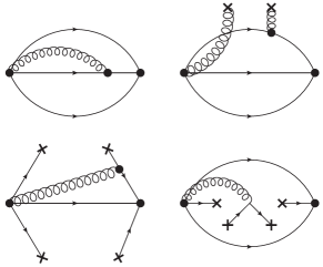
Figure 10: Leading-order contributions to the OPE of the correlation functions in Eq. (LABEL:A:CF).

The sum rules are derived from the matching of the QCD calculation of the invariant functions $\Pi^{g}_{k}(p^{2})$ at Euclidean $p^{2}\sim-1$ GeV² with the dispersion integral representation where the nucleon contribution is written explicitly:

$$\Pi^{g}_{1}(p^{2}) = \phantom{-}\frac{1}{4}m_{N}^{2}\frac{(\lambda_{2}^{g}-\lambda_{3}^{g}/3)\lambda_{1}}{m_{N}^{2}-p^{2}}+\ldots\,$$

$$\Pi^{g}_{2}(p^{2}) = \phantom{-}\frac{1}{6}m_{N}^{2}\frac{(\lambda_{2}^{g}+\lambda_{3}^{g})\lambda_{1}}{m_{N}^{2}-p^{2}}+\ldots\,$$

$$\Pi^{g}_{2}(p^{2}) = -\frac{1}{6}m_{N}^{2}\frac{(\lambda_{1}^{g}+\lambda_{3}^{g})\lambda_{2}}{m_{N}^{2}-p^{2}}+\ldots$$ (A.120)

and the contributions of higher states and the continuum are modelled in the usual way as the QCD spectral density above a certain threshold, $\sqrt{s_{0}}\sim 1.5$ GeV, dubbed the interval of duality. On the QCD side, we take into account contributions of perturbation theory and vacuum condensates of dimension 4 and 6 shown in Fig. 10. The leading-order contributions of dimension 8 vanish for all cases.

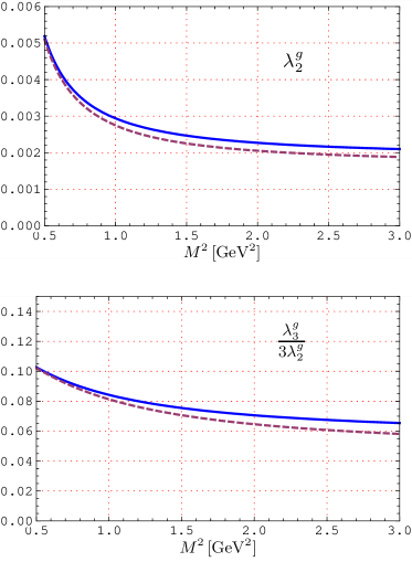
Figure 11: The coupling $\lambda_{2}^{g}$ (in units of $\text{GeV}^{2}$) (upper panel) and the ratio $\lambda_{3}^{g}/(3\lambda_{2}^{g})$ (lower panel) as a function of the Borel parameter $M^{2}$ for the central values of the condensates (A), $\alpha_{s}(1$ GeV)=0.5. The solid line corresponds to $\sqrt{s_{0}}=1.4$ GeV and the dashed line to $\sqrt{s_{0}}=1.6$ GeV.

Proceeding with the standard technique we derive the following set of sum rules:

$$2(2\pi)^{4}(\lambda_{2}^{g}-\lambda_{3}^{g}/3)\lambda_{1}m_{N}^{2}e^{-\frac{m_{N}^{2}}{M^{2}}}=$$

$${}\hskip 28.45274pt=-\frac{\alpha_{s}}{45\pi}M^{6}E_{3}-\frac{b}{12}M^{2}E_{1}-\frac{8\alpha_{s}}{9\pi}a^{2},$$

$$2(2\pi)^{4}(\lambda_{2}^{g}+\lambda_{3}^{g})\lambda_{1}m_{N}^{2}\,e^{-\frac{m_{N}^{2}}{M^{2}}}=$$

$${}\hskip 28.45274pt=-\frac{\alpha_{s}}{45\pi}M^{6}E_{3}-\frac{b}{12}M^{2}E_{1}-\frac{40\alpha_{s}}{27\pi}a^{2},$$

$$2(2\pi)^{4}(\lambda_{1}^{g}+\lambda_{3}^{g})\lambda_{2}m_{N}^{2}\,e^{-\frac{m_{N}^{2}}{M^{2}}}=$$ (A.121)

$${}\hskip 28.45274pt=\frac{\alpha_{s}}{15\pi}M^{6}E_{3}+\frac{b}{4}M^{2}E_{1}+\frac{8\alpha_{s}}{3\pi}a^{2},$$

where $M^{2}$ is the Borel parameter,

$$E_{n}=1-e^{-\frac{s_{0}}{M^{2}}}\sum\limits_{k=0}^{n-1}\frac{1}{k!}\left(\frac{s_{0}}{M^{2}}\right)^{k}$$ (A.122)

and

$$a =-(2\pi)^{2}\langle\bar{q}q\rangle=\left(0.55\pm 0.06\right)~{}\text{GeV}^{3},$$

$$b =4\pi\langle\alpha_{s}\,F^{2}\rangle=\left(0.47\pm 0.14\right)~{}\text{GeV}^{4}.$$ (A.123)

are the quark and gluon condensates, respectively, at the scale 1 GeV.

For the numerical analysis we substitute the coupling $\lambda_{1}$ in the first two equations in (A by the square root of the “Ioffe sum rule” Ioffe:1981kw

$$2(2\pi)^{4}|\lambda_{1}|^{2}m_{N}^{2}e^{-\frac{m_{N}^{2}}{M^{2}}}=M^{6}E_{3}+\frac{b}{4}M^{2}E_{1}+\frac{a^{2}}{3}\Big{(}4-\frac{4}{3}\frac{m_{0}^{2}}{M^{2}}\Big{)},$$ (A.124)

where $m_{0}^{2}=\langle\bar{q}g\sigma Fq\rangle/\langle\bar{q}q\rangle\simeq 0.65$ GeV², and taking into account that $\lambda_{1}$ is negative (which is a convention). Assuming the “working window” in the Borel parameter $M^{2}\sim 1-2$ GeV² and taking into account uncertainties in the vacuum condensates and the continuum threshold $\sqrt{s_{0}}=1.4-1.6$ GeV, we obtain the numbers given in Eq. (46) in the text. Taking into account that to a good accuracy $\lambda_{2}=-2\lambda_{1}$, we get $\frac{2}{3}\lambda_{1}^{g}=\lambda_{2}^{g}-\lambda_{3}^{g}$. This relation holds to the approximation considered here (leading-order QCD sum rules) independent on the values of vacuum condensates and other parameters. It can, however, only be valid on a certain (low) normalization scale as the anomalous dimensions of the couplings are different, cf. (45).

References

- (1) A. V. Efremov and O. V. Teryaev, Sov. J. Nucl. Phys. 39, 962 (1984).
- (2) A. P. Bukhvostov, E. A. Kuraev and L. N. Lipatov, JETP Lett. 37, 482 (1983); Sov. Phys. JETP 60, 22 (1984).
- (3) P. G. Ratcliffe, Nucl. Phys. B 264, 493 (1986).
- (4) I. I. Balitsky and V. M. Braun, Nucl. Phys. B 311, 541 (1989).
- (5) I. I. Balitsky, V. M. Braun and A. V. Kolesnichenko, Phys. Lett. B 242, 245 (1990) [Erratum-ibid. B 318, 648 (1993)]
- (6) A. Ali, V. M. Braun and G. Hiller, Phys. Lett. B 266, 117 (1991).
- (7) J. Kodaira, Y. Yasui, K. Tanaka and T. Uematsu, Phys. Lett. B 387, 855 (1996).
- (8) J. Kodaira and K. Tanaka, Prog. Theor. Phys. 101, 191 (1999).
- (9) A. Accardi, A. Bacchetta, W. Melnitchouk and M. Schlegel, JHEP 0911, 093 (2009).
- (10) A. V. Efremov and O. V. Teryaev, Sov. J. Nucl. Phys. 36, 140 (1982).
- (11) A. V. Efremov and O. V. Teryaev, Phys. Lett. B 150, 383 (1985).
- (12) J. w. Qiu and G. Sterman, Phys. Rev. Lett. 67, 2264 (1991).
- (13) J. w. Qiu and G. Sterman, Nucl. Phys. B 378, 52 (1992).
- (14) A. Efremov, V. Korotkiian and O. Teryaev, Phys. Lett. B 348, 577 (1995).
- (15) J. w. Qiu and G. Sterman, Phys. Rev. D 59, 014004 (1998).
- (16) Y. Kanazawa and Y. Koike, Phys. Lett. B 478, 121 (2000).
- (17) Y. Kanazawa and Y. Koike, Phys. Rev. D 64, 034019 (2001).
- (18) H. Eguchi, Y. Koike and K. Tanaka, Nucl. Phys. B 763, 198 (2007).
- (19) Y. Koike and K. Tanaka, Phys. Lett. B 646, 232 (2007) [Erratum-ibid. B 668, 458 (2008)]; Phys. Rev. D 76, 011502 (2007).
- (20) Z. B. Kang, J. w. Qiu, W. Vogelsang and F. Yuan, Phys. Rev. D 78, 114013 (2008).
- (21) M. Diehl, T. Feldmann, R. Jakob and P. Kroll, Eur. Phys. J. C 8, 409 (1999).
- (22) J. Bolz and P. Kroll, Z. Phys. A 356, 327 (1996).
- (23) X. d. Ji, J. P. Ma and F. Yuan, Eur. Phys. J. C 33, 75 (2004).
- (24) V. M. Braun, A. N. Manashov and J. Rohrwild, Nucl. Phys. B 807, 89 (2009).
- (25) M. Glück, E. Reya and A. Vogt, Z. Phys. C 67, 433 (1995).
- (26) M. Glück, E. Reya and A. Vogt, Eur. Phys. J. C 5, 461 (1998).
- (27) J. B. Kogut and D. E. Soper, Phys. Rev. D 1, 2901 (1970).
- (28) S. J. Brodsky, H. C. Pauli and S. S. Pinsky, Phys. Rept. 301, 299 (1998).
- (29) J. Bolz, R. Jakob, P. Kroll, M. Bergmann and N. G. Stefanis, Z. Phys. C 66, 267 (1995).
- (30) G. P. Lepage and S. J. Brodsky, Phys. Rev. D 22, 2157 (1980).
- (31) B. Pasquini, S. Cazzaniga and S. Boffi, Phys. Rev. D 78, 034025 (2008).
- (32) V. Braun, R. J. Fries, N. Mahnke et al., Nucl. Phys. B589 , 381 (2000).
- (33) In Braun:2008ia we used the definition of the matrix from: M. F. Sohnius, Phys. Rept. 128 , 39 (1985), which differs in sign from the standard definition (35) adopted in Braun:2000kw and also in this work.
- (34) V. M. Braun, S. E. Derkachov, G. P. Korchemsky and A. N. Manashov, Nucl. Phys. B 553, 355 (1999).
- (35) V. M. Braun, G. P. Korchemsky and D. Mueller, Prog. Part. Nucl. Phys. 51, 311 (2003).
- (36) V. L. Chernyak, I. R. Zhitnitsky, Nucl. Phys. B246, 52 (1984).
- (37) I. D. King, C. T. Sachrajda, Nucl. Phys. B279, 785 (1987).
- (38) V. L. Chernyak, A. A. Ogloblin, I. R. Zhitnitsky, Z. Phys. C42, 569 (1989).
- (39) V. M. Braun, A. Lenz, M. Wittmann, Phys. Rev. D73, 094019 (2006).
- (40) M. Gruber, arXiv:1011.0758 [hep-ph].
- (41) V. M. Braun et al. [QCDSF Collaboration], Phys. Rev. D 79, 034504 (2009).
- (42) V. M. Braun et al., [QCDSF Collaboration], arXiv:1011.1092 [hep-lat].
- (43) M. A. Shifman, A. I. Vainshtein and V. I. Zakharov, Nucl. Phys. B 147, 385 (1979).
- (44) B. L. Ioffe, Nucl. Phys. B 188, 317 (1981) [Erratum-ibid. B 191, 591 (1981)].
- (45) Y. Chung, H. G. Dosch, M. Kremer and D. Schall, Nucl. Phys. B 197, 55 (1982).
- (46) V. M. Braun, G. P. Korchemsky and A. N. Manashov, Nucl. Phys. B 597, 370 (2001).
- (47) V. M. Braun, A. N. Manashov and B. Pirnay, Phys. Rev. D 80, 114002 (2009).
- (48) M. Diehl, Phys. Rept. 388, 41 (2003).
- (49) D. de Florian, R. Sassot, M. Stratmann and W. Vogelsang, Phys. Rev. D 80, 034030 (2009).
- (50) E. Leader, A. V. Sidorov and D. B. Stamenov, arXiv:1010.0574 [hep-ph].
- (51) The scale dependence of parton densities on this plot was calculated using the code from: A. Cafarella, C. Coriano, Comput. Phys. Commun. 160, 213 (2004).
- (52) J. Soffer, Phys. Rev. Lett. 74, 1292 (1995).
- (53) X. Artru, M. Elchikh, J. M. Richard et al., Phys. Rept. 470, 1 (2009).
- (54) M. Anselmino, M. Boglione, U. D’Alesio et al., Phys. Rev. D75 , 054032 (2007).
- (55) M. Anselmino, M. Boglione, U. D’Alesio et al., [arXiv:0707.1197 [hep-ph]].
- (56) M. Anselmino, M. Boglione, U. D’Alesio et al., [arXiv:0807.0173 [hep-ph]].
- (57) V. Barone, A. Drago, P. G. Ratcliffe, Phys. Rept. 359 , 1 (2002).
- (58) R. L. Jaffe, Nucl. Phys. B 229, 205 (1983).
- (59) H. Burkhardt, W. N. Cottingham, Annals Phys. 56, 453 (1970).
- (60) A. V. Efremov, O. V. Teryaev, E. Leader, Phys. Rev. D55, 4307 (1997).
- (61) P. L. Anthony et al. [E155 Collaboration], Phys. Lett. B 553, 18 (2003).
- (62) K. Abe et al. [E143 collaboration], Phys. Rev. D 58, 112003 (1998).
- (63) X. Zheng et al. [Jefferson Lab Hall A Collaboration], Phys. Rev. C 70, 065207 (2004).
- (64) K. Kramer et al., Phys. Rev. Lett. 95, 142002 (2005).
- (65) M. Göckeler et al., Phys. Rev. D 63, 074506 (2001).
- (66) E. Stein, P. Gornicki, L. Mankiewicz, A. Schäfer and W. Greiner, Phys. Lett. B 343, 369 (1995).
- (67) M. Wakamatsu, Phys. Lett. B 487, 118 (2000).
- (68) V. M. Braun, G. P. Korchemsky and A. N. Manashov, Nucl. Phys. B 603, 69 (2001).
- (69) Z. B. Kang and J. W. Qiu, Phys. Rev. D 79, 016003 (2009).
- (70) C. Kouvaris, J. -W. Qiu, W. Vogelsang, F. Yuan, Phys. Rev. D74, 114013 (2006).
- (71) K. Kanazawa, Y. Koike, Phys. Rev. D82, 034009 (2010).