Abstract

An important application of distance geometry to biochemistry studies the embeddings of the vertices of a weighted graph in the three-dimensional Euclidean space such that the edge weights are equal to the Euclidean distances between corresponding point pairs. When the graph represents the backbone of a protein, one can exploit the natural vertex order to show that the search space for feasible embeddings is discrete. The corresponding decision problem can be solved using a binary tree based search procedure which is exponential in the worst case. We discuss assumptions that bound the search tree width to a polynomial size.
Keywords: Branch-and-Prune, symmetry, distance geometry.

1 Introduction

We study the following decision problem [5]:

Discretizable Molecular Distance Geometry Problem (DMDGP). Given a simple undirected weighted graph $G=(V,E,d)$ where $d:E\to\mathbb{R}_{+}$, $V$ is ordered so that $V=[n]=\{1,\ldots,n\}$, and the following assumptions hold:

1. for all $v>3$ and $u\in V$ with $1\leq v-u\leq 3$, $\{u,v\}\in E$ (Discretization)

2. for all $v>3$, $E$ contains all edges $\{u,w\}$ with $u\not=w\in U_{v}=\{u\in V\;|\;1\leq v-u\leq 3\}$, and the distances $d_{uw}$ with $u\not=w\in U_{v}$ obey the strict simplex inequalities [1] (Strict Simplex Inequalities),

and given an embedding $x^{\prime}:[3]\to\mathbb{R}^{3}$, is there an embedding $x:V\to\mathbb{R}^{3}$ extending $x^{\prime}$, such that

$$\forall\{u,v\}\in E\quad\|x_{u}-x_{v}\|=d_{uv}\;?$$ (1)

Note that the strict simplex inequalities in $\mathbb{R}^{3}$ reduce to the strict triangular inequalities $d_{v-3,v-1}<d_{v-3,v-2}+d_{v-2,v-1}$. An embedding $x$ extends an embedding $x^{\prime}$ if $x^{\prime}$ is a restriction of $x$; an embedding is feasible if it satisfies (1). We also consider the following problem variants:

• DMDGP_K, i.e. the family of decision problems (parametrized by the positive integer $K$) obtained by replacing each symbol ‘3’ in the DMDGP definition by the symbol ‘$K$’;

• the ${}^{\mbox{\sf\scriptsize K}}$DMDGP, where $K$ is given as part of the input (rather than being a fixed constant as in the DMDGP_K).

We remark that DMDGP=DMDGP₃. Other related problems also exist in the literature, such as the Discretizable Distance Geometry Problem (DDGP) [13], where the Discretization axiom is relaxed to require that each vertex $v>K$ has at least $K$ adjacent predecessors. The original results in this paper, however, only refer to the DMDGP and its variants.

The Discretization axiom guarantees that the locus of the points embedding $v$ in $\mathbb{R}^{3}$ is the intersection of the three spheres centered at $v-3,v-2,v-1$ with radii $d_{v-3,v},d_{v-2,v},d_{v-1,v}$. If this intersection is non-empty, then it contains two points apart from a set of Lebesgue measure 0 where it may contain either one point or infinitely many. The role of the Strict Simplex Inequalities axiom is to prevent the latter case of infinitely many points. As such we might actually dispense with this axiom altogether and simply discuss results that occur with probability 1. We remark that if the intersection of the three spheres is empty, then the instance is a NO one. The Discretization axiom allows the solution of DMDGP instances using a recursive algorithm called Branch-and-Prune (BP) [9]: at level $v$, the search is branched according to the (at most two) possible positions for $v$. The BP generates a (partial) binary search tree of height $n$, each full branch of which represents a feasible embedding for the given graph.

The DMDGP and its variants are related to the Molecular Distance Geometry Problem (MDGP), which asks to find an embedding in $\mathbb{R}^{3}$ of a given weighted undirected graph. We denote the generalization of the MDGP to embeddings in $\mathbb{R}^{K}$ where $K$ is part of the input by Distance Geometry Problem (DGP), and the variants with fixed $K$ by DGP_K. The MDGP is a good model for determining the structure of molecules given a set of inter-atomic distances [10, 8]. Such distances can usually be found using Nuclear Magnetic Resonance (NMR) experiments [17], a technique which allows the detection of inter-atomic distances below 5Å. The DGP has applications in wireless sensor networks [4] and graph drawing. In general, the MDGP and DGP implicitly require a search in a continuous Euclidean space [10].

The DMDGP is a model for protein backbones. For any atom $v\in V$, the distances $d_{v-1,v}$ and $d_{v-2,v-1}$ are known because they refer to covalent bonds. Furthermore, the angle between $v-2$, $v-1$ and $v$ is known because it is adjacent to two covalent bonds, which implies that $d_{v-2,v}$ is also known by triangular geometry. In general, the distance $d_{v-3,v}$ is smaller than 5Å and can therefore be assumed to be known by NMR experiments; in practice, there are ways to find atomic orders which ensure that $d_{v-3,v}$ is known [7]. There is currently no known protein with $d_{v-3,v-1}$ being exactly equal to $d_{v-3,v-2}+d_{v-2,v-1}$ [9].

The rest of this paper is organized as follows. In Sect. 2 we describe the BP algorithm. In Sect. 3 we discuss complexity issues. Sect. 4 describes some polynomial DMDGP subclasses. We make several important contributions: an NP-hardness proof for the ${}^{\mbox{\sf\scriptsize K}}$DMDGP and the DMDGP_K (for $K>2$), a new proof that the number of feasible embeddings of DMDGP instances is a power of two, and some practically relevant polynomial cases of the DMDGP.

2 The BP algorithm

For all $v\in V$ we let $N(v)=\{u\in V\;|\;\{u,v\}\in E\}$ be the set of vertices adjacent to $v$. An embedding of a subgraph of $G$ is called a partial embedding of $G$. We denote by $X$ the set of embeddings (modulo congruences) solving a DMDGP_K (or ${}^{\mbox{\sf\scriptsize K}}$DMDGP) instance.

The BP algorithm exploits the edges guaranteed by the Discretization axiom in order to search a discrete set: vertex $v$ can be placed in at most two possible positions (the intersection of $K$ spheres in $\mathbb{R}^{K}$). Each is tested in turn and the procedure called recursively for each feasible positions. The BP exploits all other edges in the graph in order to prune some branches: a position might be feasible with respect to the distances to the $K$ immediate predecessors $v-1,\ldots,v-K$, but not necessarily with distances to other adjacent predecessors.

For a partial embedding $\bar{x}$ of $G$ and $\{u,v\}\in E$ let $S^{\bar{x}}_{uv}$ be the sphere centered at $x_{u}$ with radius $d_{uv}$.

0:  A vtx. $v\in V\smallsetminus[K]$, a partial embedding $\bar{x}=(x_{1},\ldots,x_{v-1})$, a set $X$.

1:  $P=\bigcap\limits_{u\in N(v)\atop u<v}S_{uv}^{\bar{x}}$;

2:  $\forall p\in P\;(\;(x\leftarrow(\bar{x},p))$; if ($v=n$) $X\leftarrow X\cup\{x\}$ else BP($v+1$, $x$, $X$)$\;)$.

Algorithm 1 BP($v$, $\bar{x}$, $X$)

The BP algorithm, used for solving the DMDGP and its variants, is BP($K+1$, $x^{\prime}$, $\emptyset$) (see Alg. 1), where $x^{\prime}$ is the initial embedding of the first $K$ vertices mentioned in the DMDGP definition. By the DMDGP axioms, $|P|\leq 2$. At termination, $X$ contains all embeddings (modulo congruences) extending $x^{\prime}$ [9, 5]. Embeddings $x\in X$ can be represented by sequences $\chi(x)\in\{-1,1\}^{n}$ with: (i) $\chi(x)_{i}=1$ for all $i\leq K$; (ii) for all $i>K$, $\chi(x)_{i}=-1$ if $ax_{i}<a_{0}$ and $\chi(x)_{i}=1$ if $ax_{i}\geq a_{0}$, where $ax=a_{0}$ is the equation of the hyperplane through $x_{i-K},\ldots,x_{i-1}$. For an embedding $x\in X$, $\chi(x)$ is the chirality of $x$ [2] (the formal definition of chirality actually states $\chi(x)_{0}=0$ if $ax_{i}=a_{0}$, but since this event has probability 0, we do not consider it here).

The BP (Alg. 1) can be run to termination to find all possible embeddings of $G$, or stopped after the first leaf node at level $n$ is reached, in order to find just one embedding of $G$. In the last few years we have conceived and described several BP variants targeting different problems [6], including, very recently, problems with interval-type uncertainties on some of the distance values [7]. Compared to continuous search algorithms (e.g. [12]), the performance of the BP algorithm is impressive from the point of view of both efficiency and reliability. The BP algorithm, moreover, is currently the only method able to find all embeddings for a given protein backbone.

3 Complexity

Any class of YES instances where each vertex $v$ only has distances to the $K$ immediate predecessors provides a full BP binary search tree (after level $K$), and therefore shows that the BP is an exponential-time algorithm in the worst case. One remarkable feature of the computational experiments conducted on our BP implementation [15] on protein instances is that the exponential-time behaviour of the BP algorithm was never noticed empirically. When we were able to embed protein backbones of ten thousand atoms in just over 13 seconds of CPU time (on a single core) [14], we started to suspect that protein instances might have some special properties ensuring that the BP ran in polynomial time. Specifically, using the particular structure of the protein graph, we argue in Sect. 4 that it is reasonable to expect that the BP will yield a search tree of bounded width.

Restricting $d$ to only take integer values, the DGP₁ is NP-complete by reduction from Subset-Sum, the DGP_K is (strongly) NP-hard by reduction from 3-SAT, and the DGP is (strongly) NP-hard by induction on $K$ [16]. Only the DGP₁ is NP-complete because if $d$ is integer then the YES-certificate $x$ (the embedding) can be chosen to have integer values. It is currently not known whether there is a polynomial length encoding of the algebraic numbers that can be used to show that DGP is in NP.

The DMDGP is NP-hard by reduction from Subset-Sum (Thm. 3 in [5]). We generalize that proof to the DMDGP_K. Intuitively, we exploit the fact that a subset sum instance $a_{1},\ldots,a_{N}$ with solution $s_{1},\ldots,s_{N}\in\{-1,1\}$ has $\sum_{\ell\leq N}s_{\ell}a_{\ell}=0$ (the zero-sum property) to construct a DMDGP instance with $KN+1$ points, where the zero-th point is at the origin and the $\ell$-th set of $K$ successive points is associated to $a_{\ell}$; the $j$-th point in the $\ell$-th set adds $s_{\ell}a_{\ell}$ to its $j$-th coordinate, so that the last point is again the origin (all coordinates satisfy the Subset-Sum’s zero-sum property).

3.1 Theorem

The DMDGP_K is NP-hard for all $K\geq 2$.

Proof.

Let $a=(a_{1},\ldots,a_{N})$ be an instance of Subset-Sum consisting of positive integers, and define an instance of DMDGP_K where $V=\{0,\ldots,KN\}$, $E$ includes $\{i,i+j\}$ for all $j\in\{1,\ldots,K\}$ and $i\in\{0,\ldots,KN-j\}$, and:

$$\forall i\in\{0,\ldots,KN-1\}\quad d_{i,i+1} = a_{\lfloor i/K\rfloor}$$ (2)

$$\forall j\in\{2,\ldots,K\},i\in\{0,\ldots,KN-j\}\quad d_{i,i+j} = \sqrt{\sum_{\ell=1}^{j}d_{i+\ell-1,i+\ell}^{2}}$$ (3)

$$d_{0,KN} = 0.$$ (4)

Let $s\in\{-1,1\}^{N}$ be a solution of the Subset-Sum instance $a$. We let $x_{0}=0$ and for all $i=K(\ell-1)+j>0$ we let $x_{i}=x_{i-1}+s_{\ell}a_{\ell}e_{j}$, where $e_{j}$ is the vector with a one in component $j$ and zero elsewhere. Because $\sum_{\ell\leq N}s_{\ell}a_{\ell}=0$, if $s$ solves the Subset-Sum instance $a$ then, by inspection, $x$ solves the corresponding DMDGP instance (2)-(4). Conversely, let $x$ be an embedding that solves (2)-(4), where we assume without loss of generality that $x_{0}=0$. Then (3) ensures that the line through $x_{i},x_{i-1}$ is orthogonal to the line through $x_{i-1},x_{i-2}$ for all $i>1$, and again we assume without loss of generality that, for all $j\in\{1,\ldots,K\}$, the lines through $x_{j-1},x_{j}$ are parallel to the $i$-th coordinate axis. Now consider the chirality $\chi$ of $x$: because all distance segments are orthogonal, for each $j\leq K$ the $j$-th coordinate is given by $x_{KN,j}=\sum\limits_{i\bmod K=j}\chi_{i}a_{\lfloor i/K\rfloor}$. Since $d_{0,KN}=0$, for all $j\leq K$ we have $0=x_{KN,j}=\sum_{\ell\leq N}\chi_{K(\ell-1)+j}a_{\ell}$, which implies that, for all $j\leq K$, $s^{j}=(\chi_{K(\ell-1)+j}\;|\;1\leq\ell\leq N)$ is a solution for the Subset-Sum instance $a$. ∎

3.2 Corollary

The ${}^{\mbox{\sf\scriptsize K}}$DMDGP is NP-hard.

Proof.

Every specific instance of the ${}^{\mbox{\sf\scriptsize K}}$DMDGP specifies a fixed value for $K$ and hence belongs to the DMDGP_K. Hence the result follows by inclusion. ∎

4 BP search trees with bounded width

We partition $E$ into the sets $E_{D}=\{\{u,v\}\;|\;|v-u|\leq K\}$ and $E_{P}=E\smallsetminus E_{D}$. We call $E_{D}$ the discretization edges and $E_{P}$ the pruning edges. Discretization edges guarantee that a DGP instance is in the ${}^{\mbox{\sf\scriptsize K}}$DMDGP. Pruning edges are used to reduce the BP search space by pruning its tree. In practice, pruning edges might make the set $P$ in Alg. 1 have cardinality 0 or 1 instead of 2. We assume $G$ is a YES instance of the ${}^{\mbox{\sf\scriptsize K}}$DMDGP.

4.1 The discretization group

Let $G_{D}=(V,E_{D},d)$ and $X_{D}$ be the set of embeddings of $G_{D}$; since $G_{D}$ has no pruning edges, the BP search tree for $G_{D}$ is a full binary tree and $|X_{D}|=2^{n-K}$. The discretization edges arrange the embeddings so that, at level $\ell$, there are $2^{\ell-K}$ possible embeddings $x_{v}$ for the vertex $v$ with rank $\ell$. We assume that $|P|=2$ at each level $v$ of the BP tree, an event which, in absence of pruning edges, happens with probability 1 — thus many results in this section are stated with probability 1. Let $x_{v},x^{\prime}_{v}$ the possible embeddings of $v$ at level $v$ of the tree; then by elementary spherical geometry considerations, $x^{\prime}_{v}$ is the reflection of $x_{v}$ through the hyperplane defined by $x_{v-K},\ldots,x_{v-1}$. Denote this reflection by $R_{x}^{v}$.

4.1 Theorem (Cor. 4.5 and Thm. 4.8 in [11])

With probability 1, for all $v>K$ and $u<v-K$ there is a set $H^{uv}$, with $|H^{uv}|=2^{v-u-K}$, of real positive values such that for each $x\in X$ we have $\|x_{v}-x_{u}\|\in H^{uv}$. Furthermore, $\forall x\in X\;\|x_{v}-x_{u}\|=\|R_{x}^{u+K}(x_{v})-x_{u}\|$ and $\forall x^{\prime}\in X$, if $x_{v}^{\prime}\not\in\{x_{v},R_{x}^{u+K}(x_{v})\}$ then $\|x_{v}-x_{u}\|\not=\|x^{\prime}_{v}-x_{u}\|$.

Proof.

Sketched in Fig. 1 for $K=2$; the circles mark equidistant levels from 1. Intuitively, two branches from level 1 to level 4 or 5 will have equal segments but different angles, which will cause the end dots to be at different distances from level 1. The formal proof is by induction on the level distance. ∎

\psfrag{nu1}{$\nu_{1}$}\psfrag{nu2}{$\nu_{2}$}\psfrag{1}{$1$}\psfrag{2}{$2$}\psfrag{r}{$5$}\psfrag{g}{$3$}\psfrag{b}{$4$}\psfrag{3}{$\nu_{3}$}\psfrag{4}{$\nu_{4}$}\psfrag{5}{$\nu_{5}$}\psfrag{6}{$\nu_{6}$}\psfrag{7}{$\nu_{7}$}\psfrag{8}{$\nu_{8}$}\psfrag{9}{$\nu_{9}$}\psfrag{10}{$\nu_{10}$}\psfrag{11}{$\nu_{11}$}\psfrag{12}{$\nu_{12}$}\psfrag{13}{$\nu_{13}$}\psfrag{14}{$\nu_{14}$}\psfrag{15}{$\nu_{15}$}\psfrag{16}{$\nu_{16}$}\includegraphics[width=341.43306pt]{pow2}

Figure 1: A pruning edge $\{1,4\}$ prunes either $\nu_{6},\nu_{7}$ or $\nu_{5},\nu_{8}$.

We now define partial reflection operators:

$$g_{v}(x)=(x_{1},\ldots,x_{v-1},R_{x}^{v}(x_{v}),\ldots,R_{x}^{v}(x_{n})).$$ (5)

The $g_{v}$’s map an embedding $x$ to its partial reflection with first branch at $v$. It is evident that the $g_{v}$’s are injective with probability 1 and idempotent.

4.2 Lemma

For $u,v\in V$ such that $u,v>K$, $g_{u}g_{v}(x)=g_{v}g_{u}(x)$.

Proof.

Assume without loss of generality $u<v$. Then:

$$g_{u}g_{v}(x) = g_{u}(x_{1},\ldots,x_{v-1},R_{x}^{v}(x_{v}),\ldots,R_{x}^{v}(x_{n}))$$

$$= (x_{1}\ldots,x_{u-1},R_{g_{v}(x)}^{u}(x_{u}),\ldots,R_{g_{v}(x)}^{u}R_{x}^{v}(x_{v}),\ldots,R_{g_{v}(x)}^{u}R_{x}^{v}(x_{n}))$$

$$= (x_{1}\ldots,x_{u-1},R_{x}^{u}(x_{u}),\ldots,R_{g_{u}(x)}^{v}R_{x}^{u}(x_{v}),\ldots,R_{g_{u}(x)}^{v}R_{x}^{u}(x_{n}))$$

$$= g_{v}(x_{1},\ldots,x_{u-1},R_{x}^{u}(x_{u}),\ldots,R_{x}^{u}(x_{n}))$$

$$= g_{v}g_{u}(x),$$

where $R_{g_{v}(x)}^{u}R_{x}^{v}(x_{w})=R_{g_{u}(x)}^{v}R_{x}^{u}(x_{w})$ for each $w\geq v$ by Lemma 4.2 in [11]. ∎

We define the discretization group to be the group $\mathcal{G}_{D}=\langle g_{v}\;|\;v>K\rangle$ generated by the $g_{v}$’s

4.3 Corollary

With probability 1, $\mathcal{G}_{D}$ is an Abelian group isomorphic to $C_{2}^{n-K}$.

For all $v>K$ let $\gamma_{v}=(1,\ldots,1,-1_{v},\ldots,-1)$ be the vector consisting of one’s in the first $v-1$ components and $-1$ in the last components. Then the $g_{v}$ actions are directly mapped onto the chirality functions.

4.4 Lemma

For all $x\in X$, $\chi(g_{v}(x))=\chi(x)\odot\gamma_{v}$, where $\odot$ is the componentwise vector multiplication.

Proof.

This follows by definition of $g_{v}$ and of chirality of an embedding. ∎

Because, by Alg. 1, each $x\in X$ has a different chirality, for all $x,x^{\prime}\in X$ there is $g\in\mathcal{G}_{D}$ such that $x^{\prime}=g(x)$, i.e. the action of $\mathcal{G}_{D}$ on $X$ is transitive. By Thm. 4.1, the distances associated to the discretization edges are invariant with respect to the discretization group.

4.2 The pruning group

Consider a pruning edge $\{u,v\}\in E_{P}$. By Thm. 4.1, with probability 1 we have $d_{uv}\in H^{uv}$, otherwise the instance could not be a YES one. Also, again by Thm. 4.1, $d_{uv}=\|x_{u}-x_{v}\|\not=\|g_{w}(x)_{u}-g_{w}(x)_{v}\|$ for all $w\in\{u+K,\ldots,v\}$ (note that distance $\|\nu_{1}-\nu_{9}\|$ in Fig. 1 is different from all its reflections $\|\nu_{1}-\nu_{h}\|$ with $h\in\{10,11,13\}$ w.r.t. $g_{4},g_{5}$). We therefore define the pruning group $\mathcal{G}_{P}=\langle g_{w}\;|\;w>K\land\forall\{u,v\}\in E_{P}\;(w\not\in\{u+K,\ldots,v\})\rangle$. It is easy to show that $\mathcal{G}_{P}\leq\mathcal{G}_{D}$. By definition, the distances associated with the pruning edges are invariant with respect to $\mathcal{G}_{P}$.

4.5 Theorem (Thm. 5.4 in [11])

The action of $\mathcal{G}_{P}$ on $X$ is transitive.

$|X|$ was shown to be a power of two with probability 1 in the unpublished technical report [11]. We provide an shorter and clearer proof.

4.6 Theorem

With probability 1, $\exists\ell\in\mathbb{N}\;|X|=2^{\ell}$.

Proof.

Since $\mathcal{G}_{D}\cong C_{2}^{n-K}$, $|\mathcal{G}_{D}|=2^{n-K}$. Since $\mathcal{G}_{P}\leq\mathcal{G}_{D}$, $|\mathcal{G}_{P}|$ divides the order of $|\mathcal{G}_{D}|$, which implies that there is an integer $\ell$ with $|\mathcal{G}_{P}|=2^{\ell}$. By Thm. 4.5, the action of $\mathcal{G}_{P}$ on $X$ only has one orbit, i.e. $\mathcal{G}_{P}x=X$ for any $x\in X$. By idempotency, for $g,g^{\prime}\in\mathcal{G}_{P}$, if $gx=g^{\prime}x$ then $g=g^{\prime}$. This implies $|\mathcal{G}_{P}x|=|\mathcal{G}_{P}|$. Thus, for any $x\in X$, $|X|=|\mathcal{G}_{P}x|=|\mathcal{G}_{P}|=2^{\ell}$. ∎

4.3 The number of nodes in function of pruning edges

Fig. 2 shows a Directed Acyclic Graph (DAG) $\mathcal{D}_{uv}$ that we use to compute the number of valid nodes in function of pruning edges between two vertices $u,v\in V$ such that $v>K$ and $u<v-K$.

\psfrag{2}{1}\psfrag{4}{2}\psfrag{8}{4}\psfrag{16}{8}\psfrag{32}{16}\psfrag{64}{32}\psfrag{v}{$v$}\psfrag{K+1}{\scriptsize$u\!\!+\!\!K\!\!-\!\!1$}\psfrag{K+2}{\scriptsize$u\!\!+\!\!K$}\psfrag{K+3}{\scriptsize$u\!\!+\!\!K\!\!+\!\!1$}\psfrag{K+4}{\scriptsize$u\!\!+\!\!K\!\!+\!\!2$}\psfrag{K+5}{\scriptsize$u\!\!+\!\!K\!\!+\!\!3$}\psfrag{K+6}{\scriptsize$u\!\!+\!\!K\!\!+\!\!4$}\psfrag{e1}{\scriptsize$0$}\psfrag{e2}{\scriptsize$1$}\psfrag{e3}{\scriptsize$2$}\psfrag{e4}{\scriptsize$3$}\psfrag{e5}{\scriptsize$4$}\psfrag{e12}{\scriptsize$0\vee 1$}\psfrag{e23}{\scriptsize$1\vee 2$}\psfrag{e34}{\scriptsize$2\vee 3$}\psfrag{e45}{\scriptsize$3\vee 4$}\psfrag{e123}{\scriptsize$0\vee 1\vee 2$}\psfrag{e234}{\scriptsize$1\vee 2\vee 3$}\psfrag{e345}{\scriptsize$2\!\vee\!3\!\vee\!4$}\psfrag{e1234}{\scriptsize$0\vee\ldots\vee 3$}\psfrag{e2345}{\scriptsize$1\vee\ldots\vee 4$}\psfrag{e12345}{\scriptsize$0\vee\ldots\vee 4$}\includegraphics[width=398.33858pt]{numsol3}

Figure 2: Number of valid BP nodes (vertex label) at level $u+K+\ell$ (column) in function of the pruning edges (path spanning all columns).

The first line shows different values for the rank of $v$ w.r.t. $u$; an arc labelled with an integer $i$ implies the existence of a pruning edge $\{u+i,v\}$ (arcs with $\vee$-expressions replace parallel arcs with different labels). An arc is unlabelled if there is no pruning edge $\{w,v\}$ for any $w\in\{u,\ldots,v-K-1\}$. The vertices of the DAG are arranged vertically by BP search tree level, and are labelled with the number of BP nodes at a given level, which is always a power of two by Thm. 4.6. A path in this DAG represents the set of pruning edges between $u$ and $v$, and its incident vertices show the number of valid nodes at the corresponding levels. For example, following unlabelled arcs corresponds to no pruning edge between $u$ and $v$ and leads to a full binary BP search tree with $2^{v-K}$ nodes at level $v$.

4.4 Polynomial DMDGP cases

For a given $G_{D}$, each possible pruning edge set $E_{P}$ corresponds to a path spanning all columns in $\mathcal{D}_{1n}$. Instances with diagonal (Prop. 4.7) or below-diagonal (Prop. 4.8) $E_{P}$ paths yield BP trees with constant width.

4.7 Proposition

If $\exists v_{0}>K$ s.t. $\forall v>v_{0}$ $\exists!u<v-K$ with $\{u,v\}\in E_{P}$ then the BP search tree width is bounded by $2^{v_{0}-K}$.

Proof.

This corresponds to a path $\mbox{\sf p}_{0}=(1,2,\ldots,2^{v_{0}-K},\ldots,2^{v_{0}-K})$ that follows unlabelled arcs up to level $v_{0}$ and then arcs labelled $v_{0}-K-1$, $v_{0}-K-1\vee v_{0}-K$, and so on, leading to nodes that are all labelled with $2^{v_{0}-K}$ (Fig. 3, left). ∎

4.8 Proposition

If $\exists v_{0}>K$ such that every subsequence $s$ of consecutive vertices $>\!\!v_{0}$ with no incident pruning edge is preceded by a vertex $v_{s}$ such that $\exists u_{s}<v_{s}\;(v_{s}-u_{s}\geq|s|\land\{u_{s},v_{s}\}\in E_{P})$, then the BP search tree width is bounded by $2^{v_{0}-K}$.

Proof.

(Sketch) This situation corresponds to a below-diagonal path, Fig. 3 (right). ∎

\psfrag{2}{\tiny 1}\psfrag{4}{\tiny 2}\psfrag{8}{\tiny 4}\psfrag{16}{\tiny 8}\psfrag{32}{\tiny 16}\psfrag{64}{\tiny 32}\psfrag{v}{}\psfrag{K+1}{}\psfrag{K+2}{}\psfrag{K+3}{}\psfrag{K+4}{}\psfrag{K+5}{}\psfrag{K+6}{}\psfrag{e1}{}\psfrag{e2}{}\psfrag{e3}{}\psfrag{e4}{}\psfrag{e5}{}\psfrag{e12}{}\psfrag{e23}{}\psfrag{e34}{}\psfrag{e45}{}\psfrag{e123}{}\psfrag{e234}{}\psfrag{e345}{}\psfrag{e1234}{}\psfrag{e2345}{}\psfrag{e12345}{}\includegraphics[width=199.16928pt]{numsol3-p0}\psfrag{2}{\tiny 1}\psfrag{4}{\tiny 2}\psfrag{8}{\tiny 4}\psfrag{16}{\tiny 8}\psfrag{32}{\tiny 16}\psfrag{64}{\tiny 32}\psfrag{v}{}\psfrag{K+1}{}\psfrag{K+2}{}\psfrag{K+3}{}\psfrag{K+4}{}\psfrag{K+5}{}\psfrag{K+6}{}\psfrag{e1}{}\psfrag{e2}{}\psfrag{e3}{}\psfrag{e4}{}\psfrag{e5}{}\psfrag{e12}{}\psfrag{e23}{}\psfrag{e34}{}\psfrag{e45}{}\psfrag{e123}{}\psfrag{e234}{}\psfrag{e345}{}\psfrag{e1234}{}\psfrag{e2345}{}\psfrag{e12345}{}\includegraphics[width=199.16928pt]{numsol3-belowp0}

Figure 3: A path $\mbox{\sf p}_{0}$ with treewidth $8$ (left) and another path below $\mbox{\sf p}_{0}$ (right).

In general, for those instances for which the BP search tree width has a $O(\log n)$ bound, the BP has a polynomial worst-case running time $O(L2^{\log n})=O(Ln)$, where $L$ is the complexity of computing $P$. Since $L$ is typically constant in $n$ [3], for such cases the BP runs in linear time $O(n)$.

Let $V^{\prime}=\{v\in V\;|\;\exists\ell\in\mathbb{N}\;(v=2^{\ell})\}$.

4.9 Proposition

If $\exists v_{0}>K$ s.t. for all $v\in V\smallsetminus V^{\prime}$ with $v>v_{0}$ there is $u<v-K$ with $\{u,v\}\in E_{P}$ then the BP search tree width at level $n$ is bounded by $2^{v_{0}}n$.

Proof.

This corresponds to a path along the diagonal $2^{v_{0}}$ apart from logarithmically many vertices in $V$ (those in $V^{\prime}$), at which levels the BP doubles the number of search nodes (Fig. 4). ∎

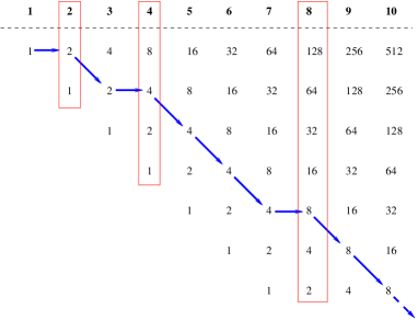
Figure 4: A path with treewidth $O(n)$.

For a pruning edge set $E_{P}$ as in Prop. 4.9, or yielding a path below it, the BP runs in quadratic time $O(n(n+1)/2)=O(n^{2})$.

4.5 Empirical verification

On a set of sixteen protein instances from the Protein Data Bank (PDB), twelve satisfy Prop. 4.7, and four Prop. 4.8, all with $v_{0}=4$. This is consistent with the computational insight [5] that BP has polynomial complexity on real proteins.

5 Conclusion

We exploit some geometrical properties of an NP-hard distance geometry problem with a specific vertex order to derive some polynomial cases. Empirically, proteins backbones seem to fall in these cases; this provides an explanation for the practical efficiency of a well-known embedding algorithm called Branch-and-Prune.

References

- [1] L. Blumenthal. Theory and Applications of Distance Geometry. Oxford University Press, Oxford, 1953.
- [2] G.M. Crippen and T.F. Havel. Distance Geometry and Molecular Conformation. Wiley, New York, 1988.
- [3] Q. Dong and Z. Wu. A geometric build-up algorithm for solving the molecular distance geometry problem with sparse distance data. Journal of Global Optimization, 26:321–333, 2003.
- [4] T. Eren, D.K. Goldenberg, W. Whiteley, Y.R. Yang, A.S. Morse, B.D.O. Anderson, and P.N. Belhumeur. Rigidity, computation, and randomization in network localization. IEEE Infocom Proceedings, pages 2673–2684, 2004.
- [5] C. Lavor, L. Liberti, N. Maculan, and A. Mucherino. The discretizable molecular distance geometry problem. Computational Optimization and Applications, in revision.
- [6] C. Lavor, L. Liberti, N. Maculan, and A. Mucherino. Recent advances on the discretizable molecular distance geometry problem. European Journal of Operational Research, submitted (invited survey).
- [7] C. Lavor, A. Mucherino, L. Liberti, and N. Maculan. On the solution of molecular distance geometry problems with interval data. In Proceedings of the International Workshop on Computational Proteomics, Hong Kong, 2010. IEEE.
- [8] C. Lavor, A. Mucherino, L. Liberti, and N. Maculan. On the computation of protein backbones by using artificial backbones of hydrogens. Journal of Global Optimization, accepted.
- [9] L. Liberti, C. Lavor, and N. Maculan. A branch-and-prune algorithm for the molecular distance geometry problem. International Transactions in Operational Research, 15:1–17, 2008.
- [10] L. Liberti, C. Lavor, A. Mucherino, and N. Maculan. Molecular distance geometry methods: from continuous to discrete. International Transactions in Operational Research, 18:33–51, 2010.
- [11] L. Liberti, B. Masson, C. Lavor, J. Lee, and A. Mucherino. On the number of solutions of the discretizable molecular distance geometry problem. Technical Report 1010.1834v1[cs.DM], arXiv, 2010.
- [12] J.J. Moré and Z. Wu. Global continuation for distance geometry problems. SIAM Journal of Optimization, 7(3):814–846, 1997.
- [13] A. Mucherino, C. Lavor, and L. Liberti. The discretizable distance geometry problem. Optimization Letters, in revision.
- [14] A. Mucherino, C. Lavor, L. Liberti, and E-G. Talbi. A parallel version of the branch & prune algorithm for the molecular distance geometry problem. In ACS/IEEE International Conference on Computer Systems and Applications (AICCSA10), Hammamet, Tunisia, 2010. IEEE conference proceedings.
- [15] A. Mucherino, L. Liberti, and C. Lavor. MD-jeep: an implementation of a branch-and-prune algorithm for distance geometry problems. In K. Fukuda, J. van der Hoeven, M. Joswig, and N. Takayama, editors, Mathematical Software, volume 6327 of LNCS, pages 186–197, New York, 2010. Springer.
- [16] J.B. Saxe. Embeddability of weighted graphs in -space is strongly NP-hard. Proceedings of 17th Allerton Conference in Communications, Control and Computing, pages 480–489, 1979.
- [17] T. Schlick. Molecular modelling and simulation: an interdisciplinary guide. Springer, New York, 2002.