Abstract

We compute the expectation values of both the time-like and the light-like Wilson loops in a strongly coupled plasma of $(p+1)$-dimensional Yang-Mills theories using gravity/gauge theory correspondence. From the time-like Wilson loop we obtain the velocity dependent quark-antiquark potential where the dipole is moving through the plasma with an arbitrary velocity $0<v<1$ and also obtain expressions for the screening lengths. When the velocity $v\to 1$, the Wilson loop becomes light-like and we obtain the form of the jet quenching parameter in those strongly coupled plasma.

1 Introduction

AdS/CFT correspondence [1, 2, 3] and its generalizations [4] help us to access the non-perturbative regimes of SU($N$) gauge theories at large $N$ simply from the low energy, weakly coupled string theory in certain backgrounds. Wilson loops are non-perturbative objects in gauge theories and the precise prescription for the computation of its expectation values using AdS/CFT correspondence has been given in [5, 6, 7, 8]. In strongly coupled gauge theories of interacting quark-gluon plasma, Wilson loops can be related to various measurable quantities in heavy ion experiments in RHIC or in LHC. For example, the expectation value of a special time-like Wilson loop can be related to the static quark-antiquark potential [9] in a moving quark-gluon plasma. On the other hand, the expectation value of a particular light-like Wilson loop can be related, among other things, to the radiative energy loss of a parton or the jet quenching parameter [10].

The velocity dependent quark-antiquark potential of a dipole moving with an arbitrary velocity through the hot quark-gluon plasma including the screening length [11, 12, 13, 14] as well as the jet quenching parameter [15, 16] have been calculated when the plasma is described by $D=4$, ${\cal N}=4$, SU($N$) Yang-Mills theory using AdS/CFT correspondence. It is of interest to see how the various quantities change if we consider Yang-Mills theories in other dimensions which are non-conformal. So, in this paper we start from the non-extremal D$p$-brane solution [20], a particular decoupling limit [21] of which defines the gravity dual of the $(p+1)$-dimensional SU($N$) Yang-Mills theory at large $N$. We then apply the fundamental string probe approach and compute the Nambu-Goto world-sheet action for this background. The expectation value of the required Wilson loop corresponds to the above minimal area whose boundary is the loop in question [5]. We consider both the time-like as well as light-like Wilson loops. We first compute the time-like Wilson loop when the velocity of the dipole is arbitrary but less than 1. From there we obtain the quark-antiquark potential of a dipole moving through the $(p+1)$-dimensional Yang-Mills plasma by performing numerical integration. This gives us exact quark-antiquark potential at different values of its velocity. This was known previously for $p=3$ in [16], but here we obtain in addition the results for $p=2,4$ and 5 as well. We have also plotted both the quark-antiquark separation and the potential for various values of $p$ at a fixed velocity to see the differences. Next we compute the screening length of the dipole not only at the leading order (as obtained in [12]), but also at the higher order in velocity and give their analytic expressions. Higher order results were known only for $p=3$ in [16] and the leading order in other $p$’s in [12] (the leading order results of the screening lengths for general $p$ were first obtained in this paper), but here we calculate the higher order corrections in screening lengths for $p=2$ and 4. We have given the results for $p=3$ also for comparison. Then we calculate the jet quenching parameter from the light-like Wilson loop, i.e. by taking the velocity going to 1 limit of the previous calculation. Our calculation is a careful rederivation of the jet quenching parameter by the method used in [16] for $p=3$ applied to other $p$’s.

This paper is organized as follows. In section 2 we compute the time-like Wilson loop and from there obtain the quark-antiquark potential as well as the screening length of the dipole moving through the $(p+1)$-dimensional Yang-Mills plasma with an arbitrary velocity. In section 3, we give the derivation of the jet quenching parameter from the light-like Wilson loop. Finally, we conclude in section 4.

2 The $q$-${\bar{q}}$ potential and the screening length

Using AdS/CFT correspondence, we calculate in this section the expectation value of the time-like Wilson loop of the $(p+1)$-dimensional Yang-Mills theory by calculating the Nambu-Goto action of a fundamental string in the background of a non-extremal D$p$-brane in a particular decoupling limit. From this we will obtain the velocity dependent quark-antiquark potential and the screening length of the dipole.

The metric (given in the string frame), the dilaton and the form-field of the non-extremal D$p$-brane solution of type II supergravity are given as [20],

$$ds^{2} = H^{-\frac{1}{2}}\left(-fdt^{2}+\sum_{i=1}^{p}(dx^{i})^{2}\right)+H^{\frac{1}{2}}\left(\frac{dr^{2}}{f}+r^{2}d\Omega_{8-p}^{2}\right)$$

$$e^{2(\phi-\phi_{0})} = H^{\frac{3-p}{2}},\qquad F_{[p+2]}=\coth\alpha\,dH^{-1}\wedge dt\wedge dx^{1}\wedge\ldots\wedge dx^{p}$$ (1)

Here the functions $H(r)$ and $f(r)$ are defined as,

$$H(r)=1+\frac{r_{0}^{7-p}\sinh^{2}\alpha}{r^{7-p}},\qquad f(r)=1-\frac{r_{0}^{7-p}}{r^{7-p}}$$ (2)

where $r_{0}$ and $\alpha$ are two parameters related to the mass and the charge of the black D$p$-brane. There is an event horizon at $r=r_{0}$ and $e^{\phi_{0}}=g_{s}$ is the string coupling constant. The form-field $F_{[p+2]}$ has to be made self-dual for $p=3$. In the decoupling limit we zoom into the region,

$$r_{0}^{7-p}<r^{7-p}\ll r_{0}^{7-p}\sinh^{2}\alpha$$ (3)

So, $\alpha$ is a very large angle and we can neglect 1 in $H(r)$, i.e.,

$$H(r)\approx\frac{r_{0}^{7-p}\sinh^{2}\alpha}{r^{7-p}}$$ (4)

and the metric now takes the form,

$$ds^{2}=\frac{r^{\frac{7-p}{2}}}{r_{0}^{\frac{7-p}{2}}\sinh\alpha}\left(-fdt^{2}+\sum_{i=1}^{p}(dx^{i})^{2}\right)+\frac{r_{0}^{\frac{7-p}{2}}\sinh\alpha}{r^{\frac{7-p}{2}}}\frac{dr^{2}}{f}+\frac{r_{0}^{\frac{7-p}{2}}\sinh\alpha}{r^{\frac{3-p}{2}}}d\Omega_{8-p}^{2}$$ (5)

Along with the other field configurations this is the gravity dual of $(p+1)$-dimensional finite temperature SU($N$) Yang-Mills theory [21]. We use open string as a probe and consider its dynamics in this background. Let the line joining the end points of the open string, i.e., the dipole lie along $x^{1}$-direction and move with an arbitrary velocity $0<v<1$ along $x^{p}$-direction. Since the dipole lies perpendicular to its direction of propagation, so $p$ must be greater than 1. Now we can go to the rest frame $(t^{\prime},\,x^{p}\,{}^{\prime})$ of the quark-antiquark by boosting the coordinate system as,

$$dt = \cosh\eta\,dt^{\prime}-\sinh\eta\,(dx^{p})^{\prime}$$

$$dx^{p} = -\sinh\eta\,dt^{\prime}+\cosh\eta\,(dx^{p})^{\prime}$$ (6)

where the boost parameter $\eta$ is related to $v$ as $\tanh\eta=v$. In this frame the dipole is static and the quark-gluon plasma is moving with velocity $v$ in the negative $x^{p}$-direction. The Wilson loop lies in the $t^{\prime}$-$x^{1}\,{}^{\prime}$ plane and we denote the lengths as ${\cal T}$ and $L$ in those directions. We further assume ${\cal T}\gg L$ such that the string world-sheet is time translation invariant. Using (2) in the metric (5) we get,

$$ds^{2} = -A(r)dt^{2}-2B(r)dtdx^{p}+C(r)(dx^{p})^{2}+\frac{r^{\frac{7-p}{2}}}{r_{0}^{\frac{7-p}{2}}\sinh\alpha}\sum_{i=1}^{p-1}(dx^{i})^{2}$$ (7)

$$\qquad\qquad\qquad\qquad\qquad+\frac{r_{0}^{\frac{7-p}{2}}\sinh\alpha}{r^{\frac{7-p}{2}}}\frac{dr^{2}}{f}+\frac{r_{0}^{\frac{7-p}{2}}\sinh\alpha}{r^{\frac{3-p}{2}}}d\Omega_{8-p}^{2}$$

$$= G_{\mu\nu}dx^{\mu}dx^{\nu}$$

where

$$A(r) = \frac{r^{\frac{7-p}{2}}}{r_{0}^{\frac{7-p}{2}}\sinh\alpha}\left(1-\frac{r_{0}^{7-p}\cosh^{2}\eta}{r^{7-p}}\right)$$

$$B(r) = \frac{r_{0}^{\frac{7-p}{2}}}{r^{\frac{7-p}{2}}\sinh\alpha}\sinh\eta\cosh\eta$$

$$C(r) = \frac{r^{\frac{7-p}{2}}}{r_{0}^{\frac{7-p}{2}}\sinh\alpha}\left(1+\frac{r_{0}^{7-p}\sinh^{2}\eta}{r^{7-p}}\right)$$ (8)

Also note that since we will be using the primed coordinates from now on, we have dropped the ‘prime’ in writing (7) for brevity. We will evaluate the world-sheet Nambu-Goto action given by,

$$S=\frac{1}{2\pi\alpha^{\prime}}\int d\sigma d\tau\sqrt{-{\rm det}g_{\alpha\beta}}$$ (9)

in this background. Here $g_{\alpha\beta}$ is the induced metric on the world-sheet

$$g_{\alpha\beta}=G_{\mu\nu}\frac{\partial x^{\mu}}{\partial\xi^{\alpha}}\frac{\partial x^{\nu}}{\partial\xi^{\beta}}$$ (10)

with $\xi^{\alpha}=\tau,\,\sigma$ for $\alpha=0,1$ respectively. We choose the static gauge condition for evaluating (9) as, $\tau=t$, $\sigma=x^{1}$, where $-L/2\leq x^{1}\leq L/2$ and $r=r(\sigma)$, $x^{2}(\sigma)=x^{3}(\sigma)=\cdots=x^{p}(\sigma)=$ constant. $r(\sigma)$ is the string embedding we want to determine with the boundary condition, $r(\pm\frac{L}{2})=r_{0}\Lambda$. Using these in (9), we get

$$S=\frac{{\cal T}}{2\pi\alpha^{\prime}}\int_{-L/2}^{L/2}d\sigma\left[A(r)\left(\frac{r^{\frac{7-p}{2}}}{r_{0}^{\frac{7-p}{2}}\sinh\alpha}+\frac{r_{0}^{\frac{7-p}{2}}\sinh\alpha}{r^{\frac{7-p}{2}}}\frac{(\partial_{\sigma}r)^{2}}{f}\right)\right]^{\frac{1}{2}}$$ (11)

Now defining new dimensionless variables $y=r/r_{0}$, and also $\tilde{\sigma}=\sigma/(r_{0}\sinh\alpha)$, $\ell=L/(r_{0}\sinh\alpha)=4\pi LT/(7-p)$, where $T$ is the Hawking temperature that can be obtained from the non-extremal D$p$-brane metric in (2) as $T=(7-p)/(4\pi r_{0}\sinh\alpha)$, the action (11) reduces to,

$$S=\frac{{\cal T}r_{0}}{\pi\alpha^{\prime}}\int_{0}^{\ell/2}d\tilde{\sigma}{\cal L}=\frac{{\cal T}d_{p}^{\frac{1}{5-p}}\lambda^{\frac{1}{5-p}}(4\pi T)^{\frac{2}{5-p}}}{\pi(7-p)^{\frac{2}{5-p}}}\int_{0}^{\ell/2}d\sigma{\cal L}$$ (12)

where

$${\cal L}=\sqrt{\left(y^{7-p}-\cosh^{2}\eta\right)\left(1+\frac{y^{\prime 2}}{y^{7-p}-1}\right)}$$ (13)

with $y^{\prime}=\partial y/\partial\sigma$. Here we have used the fact that $y$ is an even fuction of $\sigma$ by symmetry. Note that in writing the second expression in (12), we have used the standard formulae [21],

$$r_{0}^{7-p}\sinh^{2}\alpha = d_{p}g_{\rm YM}^{2}N\alpha^{\prime 5-p}=d_{p}\lambda\alpha^{\prime 5-p}$$

$$r_{0}\sinh\alpha = \frac{7-p}{4\pi T}$$ (14)

where $d_{p}=2^{7-2p}\pi^{(9-3p)/2}\Gamma((7-p)/2)$ and $\lambda=g_{\rm YM}^{2}N$, the ’t Hooft coupling, $N$ being the number of D$p$-branes which in gauge theory is the rank of the gauge group. In the above $p$ has been assumed to be less than 5. We will mention about $p=$ 5 and 6 later. Also note that in the second expression of (12), we have omitted the ‘tilde’ in $\sigma$ for brevity. $y(\sigma)$ is determined by extremizing (12). Now since the Lagrangian density given in (13) does not depend explicitly on $\sigma$, we have

$${\cal H}={\cal L}-y^{\prime}\frac{\partial{\cal L}}{\partial y^{\prime}}=\frac{y^{7-p}-\cosh^{2}\eta}{\sqrt{\left(y^{7-p}-\cosh^{2}\eta\right)\left(1+\frac{y^{\prime 2}}{y^{7-p}-1}\right)}}={\rm const.}$$ (15)

As explained in [16] for D3-brane, we will consider two cases: (i) In this case, $\cosh^{\frac{2}{7-p}}\eta<\Lambda$ and then take $\Lambda\to\infty$. So, the rapidity $\eta$ remains finite. The Wilson loop in this case is time-like and the action is real. We will compute the quark-antiquark potential and the screening length for this case in this section. (ii) In this case, initially we take $\cosh^{\frac{2}{7-p}}\eta>\Lambda$ and then take $\eta\to\infty$ keeping $\Lambda$ finite. The Wilson loop in this case would be light-like and the action is imaginary. We will take $\Lambda\to\infty$ at the end and obtain the expression for the jet quenching parameter. This will be considered in the next section.

For case (i) when $\cosh^{\frac{2}{7-p}}\eta<\Lambda$ and the action is real, let us denote the constant of motion (15) as $q$. Then $y^{\prime}$ can be solved and we get from (15),

$$y^{\prime}=\frac{1}{q}\sqrt{\left(y^{7-p}-1\right)\left(y^{7-p}-y_{c}^{7-p}\right)}$$ (16)

where $y_{c}^{7-p}=\cosh^{2}\eta+q^{2}>1$, denotes the largest turning point where $y^{\prime}$ vanishes. Integrating this equation we obtain,

$$2\int_{0}^{\ell/2}d\sigma=\ell(q)=2q\int_{y_{c}}^{\infty}\frac{dy}{\sqrt{\left(y^{7-p}-1\right)\left(y^{7-p}-y_{c}^{7-p}\right)}}$$ (17)

Note here that we have taken the boundary $\Lambda\to\infty$. Eq.(17) therefore gives us the separation between the quark and the antiquark in the dipole as a function of the integration constant $q$. The integral expression for the quark-antiquark separation for the general metric including D$p$-branes has been given in [12]. It is difficult to integrate the expression on the rhs of (17) and write an analytic expression for $\ell(q)$ in general. However, we can give analytic expression for large rapidity $\eta$ or large $y_{c}$ and from there we can obtain the form of screening length which will be discussed later.

Now substituting the form of $y^{\prime}$ from (16) into the action (12) along with (13) and changing the variable from $\sigma$ to $y$, we get,

$$S(\ell)=\frac{{\cal T}d_{p}^{\frac{1}{5-p}}\lambda^{\frac{1}{5-p}}(4\pi T)^{\frac{2}{5-p}}}{\pi(7-p)^{\frac{2}{5-p}}}\int_{y_{c}}^{\infty}dy\frac{y^{7-p}-\cosh^{2}\eta}{\sqrt{\left(y^{7-p}-1\right)\left(y^{7-p}-y_{c}^{7-p}\right)}}$$ (18)

Note that here we have expressed $S$ completely in terms of the parameters of the gauge theory. In order to calculate the quark-antiquark potential we must subtract from it the quark and antiquark self-energy $S_{0}$. If $E(L)$ is the potential then,

$$E(L)=\frac{S(\ell)-S_{0}}{\cal T}$$ (19)

Now to compute $S_{0}$, we consider an open string along radial direction, i.e. a single quark in the same background (7) as before and use the static gauge condition $\tau=t$, $\sigma=r$, $x^{p}=x^{p}(\sigma)$ and $x^{1}(\sigma)=x^{2}(\sigma)=\cdots=x^{p-1}(\sigma)=$ constant. With these we evaluate the Nambu-Goto world-sheet action and then multiply by 2 to get the contribution for two strings. From (9) we get in this case,

$$S_{0}=\frac{2{\cal T}}{2\pi\alpha^{\prime}}\int_{r_{0}}^{\infty}dr\sqrt{\frac{r_{0}^{\frac{7-p}{2}}\sinh\alpha}{r^{\frac{7-p}{2}}}\frac{A(r)}{f}+\left(A(r)C(r)+B(r)^{2}\right)(x^{p}\,{}^{\prime})^{2}}$$ (20)

where $A(r)$, $B(r)$ and $C(r)$ are as given before in (2). Note here that the string stretches all the way upto the horizon $r_{0}$. Now introducing new dimensionless variables as before $y=r/r_{0}$ and $z=x^{p}/(r_{0}\sinh\alpha)$ and substituting $r_{0}/\alpha^{\prime}$ in terms of the parameters of the gauge theory we get from (20),

$$S_{0}=\frac{{\cal T}d_{p}^{\frac{1}{5-p}}\lambda^{\frac{1}{5-p}}(4\pi T)^{\frac{2}{5-p}}}{\pi(7-p)^{\frac{2}{5-p}}}\int_{1}^{\infty}dy\sqrt{\frac{y^{7-p}-\cosh^{2}\eta}{y^{7-p}-1}+\left(y^{7-p}-1\right)\left(\frac{\partial z}{\partial y}\right)^{2}}$$ (21)

Since the Lagrangian density in (21) is independent of $z$, the Euler-Lagrange equation of motion gives a conservation relation $(\partial{\cal L}/\partial(\partial_{y}z))=$ const. independent of $y$. Denoting the constant by $\tilde{q}$, we get from this,

$$\left(\frac{\partial z}{\partial y}\right)^{2}=\tilde{q}^{2}\frac{y^{7-p}-\cosh^{2}\eta}{\left(y^{7-p}-1\right)^{2}\left(y^{7-p}-\tilde{q}^{2}-1\right)}$$ (22)

Since $y$ varies from 1 to $\infty$, the right hand side can become negative and unphysical for arbitrary values of $\eta$ and $\tilde{q}$. So, in order to get physical solution we must choose the constant $\tilde{q}=\sinh\eta$. Therefore, we get

$$\frac{\partial z}{\partial y}=\frac{\sinh\eta}{\left(y^{7-p}-1\right)}\quad\Rightarrow\quad z(y)={\rm const.}-y\sinh\eta\,\,_{2}F_{1}\left(1,\frac{1}{7-p},\frac{8-p}{7-p};y^{7-p}\right)$$ (23)

where ${}_{2}F_{1}$ is the hypergeometric function. Now substituting $\partial z/\partial y$ into (21) we get

$$S_{0}=\frac{{\cal T}d_{p}^{\frac{1}{5-p}}\lambda^{\frac{1}{5-p}}(4\pi T)^{\frac{2}{5-p}}}{\pi(7-p)^{\frac{2}{5-p}}}\int_{1}^{\infty}dy$$ (24)

So, the quark-antiquark potential (19) has the form,

$$E(\ell)=\frac{d_{p}^{\frac{1}{5-p}}\lambda^{\frac{1}{5-p}}(4\pi T)^{\frac{2}{5-p}}}{\pi(7-p)^{\frac{2}{5-p}}}\left[\int_{y_{c}}^{\infty}dy\left(\frac{y^{7-p}-\cosh^{2}\eta}{\sqrt{(y^{7-p}-1)(y^{7-p}-y_{c}^{7-p})}}-1\right)-(y_{c}-1)\right]$$ (25)

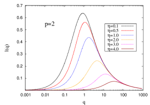
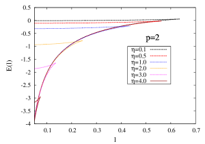
Figure 1: (a) shows the plot of quark-antiquark separation $\ell$ as a function of integration const. $q$ for $p=2$ at different rapidities $\eta$ of the dipole. (b) shows the plot of properly normalized quark-antiquark potential as a function of $\ell$ for $p=2$ at the same set of rapidities.

It is in general not possible to perform the integration on the rhs of (25) and obtain an analytic expression for quark-antiquark potential $E(\ell)$. So, as in [16, 11], we will first plot $\ell(q)$ vs $q$ for certain particular values of $\eta$ from the integral equation (17) and obtain $q$ as a function of $\ell$ and then using these $q$ in the integral equation (25) we plot $E(\ell)$ vs $\ell$ for those values of $\eta$. In [16, 11], these plots were given for $p=3$, we here give the plots for $p=2,\,4$ and 5 in Figures 1, 2 and 3 respectively. Also for comparison with different $p$’s (including $p=3$) we give the plot of both $\ell(q)$ vs $q$ and $E(\ell)$ vs $\ell$ in Figure 4 at $\eta=1$.

We have mentioned before that we are mainly considering the cases with $p<5$. This is because the constant (expressed in terms of the parameters of the gauge theory by (2)) in front of the second expression in (12) is ill defined for $p=5$. But no such problem arises if we keep the parameters $r_{0}$ and $\alpha^{\prime}$ as in the first expression in (12) of the gravity theory. In fact we see from (2) that for $p=5$ we can not express $r_{0}/\alpha^{\prime}$ in terms of the parameters of the gauge theory. This may be an indication that in this case the complete decoupling does not occur. However, we can still plot $\ell(q)$ vs $q$ and $E(\ell)$ vs $\ell$, as we do for $p=5$, keeping the constant in terms of the parameters of the gravity side. Even for $p=6$ case, it is known that the decoupling does not occur and so, we do not plot the functions.

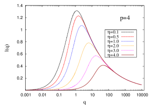
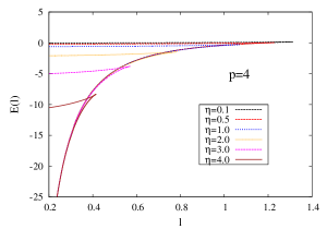
Figure 2: (a) shows the plot of quark-antiquark separation $\ell$ as a function of integration const. $q$ for $p=4$ at different rapidities $\eta$ of the dipole. (b) shows the plot of properly normalized quark-antiquark potential as a function of $\ell$ for $p=4$ at the same set of rapidities.

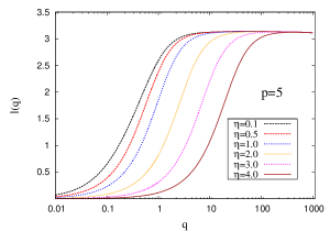
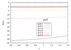
Figure 3: (a) shows the plot of quark-antiquark separation $\ell$ as a function of integration const. $q$ for $p=5$ at different rapidities $\eta$ of the dipole. Here $\ell$ saturates unlike in Figures 1 and 2. (b) shows the plot of properly normalized quark-antiquark potential as a function of $\ell$ for $p=5$ at the same set of rapidities. There is no lower branch unlike in Figures 1 and 2.

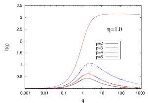
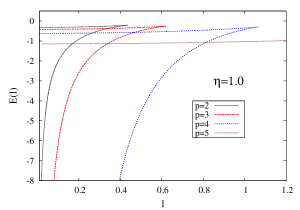
Figure 4: (a) shows the plot of quark-antiquark separation $\ell$ as a function of integration const. $q$ for different values of $p$ for comparison at $\eta=1.0$. (b) shows the plot of quark-antiquark potential as a function of $\ell$ for different values of $p$ for comparison at the same $\eta=1.0$.

The general features of the plot for $p=2,\,4$ remain very similar (although the details, as shown in Figure 4 below, are quite different) to $p=3$ case discussed in [16, 11]. It is clear from (17) that $\ell(q)$ goes to zero as $q$ for small $q$ (for all $p$) and as $q^{-(5-p)/(7-p)}$ for large $q$ (for $p<5$). However, for $p=5$, it goes to a constant for large $q$. These can be seen in Figures 1, 2, 3. Also, for $p<5$, the plots show that it has a maximum $\ell_{\rm max}$ in between. Beyond this there is no solution of (17). From Figures 1, 2 we see that the peak of the $\ell(q)$ curve reduces and shifts towards right, i.e, towards a larger value of $q$ as we increase $\eta$ or the rapidity. From Figure 4(a), we see that at a fixed value of $\eta$, the peak reduces as we increase $p$ and shifts towards left i.e., towards a lower value of $q$. As $\ell(q)$ decreases from $\ell_{\rm max}$, there are two dipoles at a fixed $\ell$ for two different values of $q$. The quark-antiquark potential in general decreases with increasing values of $\eta$ at each $p$ and has two branches corresponding to the two values of $q$. The smaller value of $q$ corresponds to the upper branch and has higher energy, whereas the larger value of $q$ corresponds to the lower branch and has lower energy. So, the dipole with lower $q$ will be metastable and will go to the state with higher $q$ as it is energetically more favorable.

Also, there exists a critical $\eta_{c}$ above which the whole upper branch of the $E(\ell)$ curve is negative. But for $\eta<\eta_{c}$ the $E(\ell)$ curve crosses zero at $\ell=\ell_{c}$, continues to rise till $\ell=\ell_{\rm max}$ and turns back crossing zero again at $\ell=\ell^{\prime}_{c}>\ell_{c}$. Below $\ell_{c}$, the upper branch is metastable. A dipole on the upper branch on slight perturbation will come down to the lower branch. At $\ell=\ell_{c}$, the dipole in the upper branch and the two isolated string configurations (or dissociated quark and antiquark) have the same energy. So, both the states can coexist. However with slight disturbance it will settle down to the dipole in the lower branch. In the regime $\ell_{c}<\ell<\ell^{\prime}_{c}$ the upper branch has positive energy while the lower one has negative energy. So a dipole sitting on the upper branch, when perturbed, may either come down and settle in the lower branch or it may dissociate into a free quark and a free antiquark. At $\ell=\ell^{\prime}_{c}$, the dipole in the lower branch and the two isolated string states (or dissociated quark and antiquark) can coexist and both are stable configurations. In the domain $\ell^{\prime}_{c}<\ell<\ell_{\rm max}$ both the branches have positive energy and so a dipole sitting on either of them will dissociate when slightly disturbed. Beyond $\ell_{\rm max}$ no dipole will be formed at all.

Some of these features were mentioned in [16, 11] for $p=3$, but it continues to hold for $p=2,\,4$ cases as well. For $p=5$, since there is no maximum for $\ell(q)$ plot, there is no lower branch in the $E(\ell)$ vs $\ell$ plot. The plot of quark-antiquark potential $E(\ell)$ for different values of $p$ are given in Figure 4(b) for comparison.

We mentioned before that $\ell(q)$ in (17) can not be integrated in general. However, for large $\eta$ or large $y_{c}$, we can expand $\ell(q)$ and then integrate to write a series expansion in powers of $1/y_{c}$ as,

$$\ell(q) = 2q\int_{y_{c}}^{\infty}\frac{dy}{y^{\frac{7-p}{2}}(y^{7-p}-y_{c}^{7-p})^{\frac{1}{2}}}+q\int_{y_{c}}^{\infty}\frac{dy}{y^{\frac{3(7-p)}{2}}(y^{7-p}-y_{c}^{7-p})^{\frac{1}{2}}}$$ (26)

$$\qquad\qquad+\frac{3q}{4}\int_{y_{c}}^{\infty}\frac{dy}{y^{\frac{5(7-p)}{2}}(y^{7-p}-y_{c}^{7-p})^{\frac{1}{2}}}+\cdots$$

and on integration this yields for $p=2,\,3$ and 4,

$$\ell(q)^{p=2} = \frac{2q\sqrt{\pi}}{5y_{c}^{4}}\left[\frac{\Gamma(\frac{4}{5})}{\Gamma(\frac{13}{10})}+\frac{\Gamma(\frac{9}{5})}{10\Gamma(\frac{23}{10})}\frac{1}{y_{c}^{5}}+\frac{3\Gamma(\frac{14}{5})}{8\Gamma(\frac{33}{10})}\frac{1}{y_{c}^{10}}+\cdots\right]$$ (27)

$$\ell(q)^{p=3} = \frac{2q\sqrt{\pi}}{y_{c}^{3}}\left[\frac{\Gamma(\frac{3}{4})}{\Gamma(\frac{1}{4})}+\frac{\Gamma(\frac{7}{4})}{8\Gamma(\frac{9}{4})}\frac{1}{y_{c}^{4}}+\frac{3\Gamma(\frac{11}{4})}{32\Gamma(\frac{13}{4})}\frac{1}{y_{c}^{8}}+\cdots\right]$$ (28)

$$\ell(q)^{p=4} = \frac{4q\sqrt{\pi}}{y_{c}^{2}}\left[\frac{\Gamma(\frac{2}{3})}{\Gamma(\frac{1}{6})}+\frac{\Gamma(\frac{5}{3})}{12\Gamma(\frac{13}{6})}\frac{1}{y_{c}^{3}}+\frac{\Gamma(\frac{8}{3})}{16\Gamma(\frac{19}{6})}\frac{1}{y_{c}^{6}}+\cdots\right]$$ (29)

By truncating the series upto the second term we can calculate $\ell_{\rm max}$ for the above three cases as,

$$\ell_{\rm max}^{p=2} = \frac{2\,\cdot 3^{3/10}\sqrt{\pi}\Gamma(\frac{4}{5})}{8^{4/5}\sqrt{5}\Gamma(\frac{13}{10})}\left[\frac{1}{\cosh^{\frac{3}{5}}\eta}+\frac{3}{130}\frac{1}{\cosh^{\frac{13}{5}}\eta}+\cdots\right]$$ (30)

$$= 0.54176\left[\frac{1}{\cosh^{\frac{3}{5}}\eta}+\frac{3}{130}\frac{1}{\cosh^{\frac{13}{5}}\eta}+\cdots\right]$$

$$\ell_{\rm max}^{p=3} = \frac{2\sqrt{2\pi}\Gamma(\frac{3}{4})}{3^{3/4}\Gamma(\frac{1}{4})}\left[\frac{1}{\cosh^{\frac{1}{2}}\eta}+\frac{1}{10}\frac{1}{\cosh^{\frac{5}{2}}\eta}+\cdots\right]$$ (31)

$$= 0.74333\left[\frac{1}{\cosh^{\frac{1}{2}}\eta}+\frac{1}{10}\frac{1}{\cosh^{\frac{5}{2}}\eta}+\cdots\right]$$

$$\ell_{\rm max}^{p=4} = \frac{4^{1/3}\sqrt{3\pi}\Gamma(\frac{2}{3})}{\Gamma(\frac{1}{6})}\left[\frac{1}{\cosh^{\frac{1}{3}}\eta}+\frac{1}{14}\frac{1}{\cosh^{\frac{7}{3}}\eta}+\cdots\right]$$ (32)

$$= 1.18553\left[\frac{1}{\cosh^{\frac{1}{3}}\eta}+\frac{1}{14}\frac{1}{\cosh^{\frac{7}{3}}\eta}+\cdots\right]$$

The quantity $L_{\rm max}=(7-p)\ell_{\rm max}/(4\pi T)$ can be thought of as the screening length of the dipole in the medium since this is the maximum value of $L$ beyond which we have two dissociated quark and antiquark or two disjoint world-sheet corresponding to $E(L)=0$. It has been pointed out in [11, 16] for $p=3$ that if we set $\eta=0$ in the above result (31) which was derived for large $\eta$ is not too far off from the actual result at $\eta=0$ and so the screening length decreases with increasing velocity according to the scaling $L^{p=3}_{\rm max}(v)\simeq L^{p=3}_{\rm max}(0)/\cosh^{1/2}\eta=L^{p=3}_{\rm max}(0)/\sqrt{\gamma}$, where $\gamma=1/\sqrt{1-v^{2}}$. By looking at the similarity of the behavior of $\ell(q)$ and $E(\ell)$ for $p=2,\,4$, with $p=3$, we may conclude that similar behavior will also hold true for $p=2,\,4$ cases as well. Then the velocity dependence of the screening lengths in these two cases is of the form,

$$L^{p=2}_{\rm max}(v) \simeq \frac{L^{p=2}_{\rm max}(0)}{\cosh^{\frac{3}{5}}\eta}=\frac{L^{p=2}_{\rm max}(0)}{\gamma^{\frac{3}{5}}}$$ (33)

$$L^{p=4}_{\rm max}(v) \simeq \frac{L^{p=4}_{\rm max}(0)}{\cosh^{\frac{1}{3}}\eta}=\frac{L^{p=4}_{\rm max}(0)}{\gamma^{\frac{1}{3}}}$$ (34)

A general expression for the leading order contribution of the screening lengths for general $p$ has been given in [12]. This concludes our discussion on time-like Wilson loop when $\cosh^{\frac{2}{7-p}}\eta<\Lambda$ and $\eta$ remains finite while $\Lambda\to\infty$.

3 The jet quenching parameter

So far in our discussion we assumed that the rapidity $\eta$ is finite and $\cosh^{\frac{2}{7-p}}\eta<\Lambda$. So, the velocity of the string is in the range $0<v<1$ and the Wilson loop is time-like. Now we will consider case (ii), i.e., $\cosh^{\frac{2}{7-p}}\eta>\Lambda$. In order to extract the jet quenching parameter we take $\eta\to\infty$ or $v\to 1$, so that the Wilson loop is light-like and then take $\Lambda\to\infty$. (We will be brief here since the jet quenching parameter for $(p+1)$-dimensional Yang-Mills theory has already been given in [16, 15]. But here we obtain it by taking $v\to 1$ limit of the time-like Wilson loop at $0<v<1$ as was done there for $p=3$ case.) Note from (12) that since now $\cosh^{\frac{2}{7-p}}\eta>\Lambda$, the action is imaginary and we write the second expression in (12) as,

$$S=i\frac{{\cal T}d_{p}^{\frac{1}{5-p}}\lambda^{\frac{1}{5-p}}(4\pi T)^{\frac{2}{5-p}}}{\pi(7-p)^{\frac{2}{5-p}}}\int_{0}^{\ell/2}d\sigma{\cal L}$$ (35)

where

$${\cal L}=\sqrt{\left(\cosh^{2}\eta-y^{7-p}\right)\left(1+\frac{y^{\prime 2}}{y^{7-p}-1}\right)}$$ (36)

As before since the Lagrangian density (36) does not explicitly depend on $\sigma$, the corresponding Hamiltonian is conserved. So, we have,

$${\cal H}={\cal L}-y^{\prime}\frac{\partial{\cal L}}{\partial y^{\prime}}={\rm const.}\quad\Rightarrow\quad\frac{\cosh^{2}\eta-y^{7-p}}{\sqrt{(\cosh^{2}\eta-y^{7-p})\left(1+\frac{y^{\prime 2}}{y^{7-p}-1}\right)}}=q_{0}$$ (37)

where we have denoted the constant as $q_{0}$. The equation (37) can be solved for $y^{\prime}$ as,

$$y^{\prime}=\frac{1}{q_{0}}\sqrt{(y^{7-p}-1)(y_{m}^{7-p}-y^{7-p})}$$ (38)

where $y_{m}^{7-p}=\cosh^{2}\eta-q_{0}^{2}$. On integration eq.(38) gives us,

$$\ell=2q_{0}\int_{1}^{\Lambda}\frac{dy}{\sqrt{(y_{m}^{7-p}-y^{7-p})(y^{7-p}-1)}}$$ (39)

Substituting the value of $y^{\prime}$ from (38) into the action (35) we get,

$$S(\ell)=i\frac{{\cal T}d_{p}^{\frac{1}{5-p}}\lambda^{\frac{1}{5-p}}(4\pi T)^{\frac{2}{5-p}}}{\pi(7-p)^{\frac{2}{5-p}}}\int_{1}^{\Lambda}dy\frac{\cosh^{2}\eta-y^{7-p}}{\sqrt{(y_{m}^{7-p}-y^{7-p})(y^{7-p}-1)}}$$ (40)

So far we have used only $\cosh^{\frac{2}{7-p}}\eta>\Lambda$. Now for large $\eta$, $\ell$ in (39) can be expanded as follows,

$$\ell=\frac{2q_{0}}{\cosh\eta}\int_{1}^{\Lambda}\frac{dy}{\sqrt{y^{7-p}-1}}+O(\frac{q_{0}^{3}}{\cosh^{3}\eta},\frac{\Lambda^{7-p}}{\cosh^{3}\eta})$$ (41)

Next, as we take $\eta\to\infty$ the second term in (41) drops out and then taking $\Lambda\to\infty$ we get,

$$\ell=\frac{2q_{0}}{\cosh\eta}a_{p},\qquad{\rm with,}\quad a_{p}=\frac{2}{5-p}\sqrt{\pi}\frac{\Gamma\left(1+\frac{5-p}{2(7-p)}\right)}{\Gamma\left(\frac{6-p}{7-p}\right)}$$ (42)

Further, since $L$ is much smaller than the other length dimensions of the problem $\ell=(4\pi LT)/(7-p)\ll 1$ and therefore $q_{0}=(\ell\cosh\eta)/(2a_{p})\ll 1$. In this limit, $S(\ell)$ in (40) can be expanded as,

$$S(\ell)=S^{(0)}+q_{0}^{2}S^{(1)}+O(q_{0}^{4})$$ (43)

where

$$S^{(0)} = i\frac{{\cal T}d_{p}^{\frac{1}{5-p}}\lambda^{\frac{1}{5-p}}(4\pi T)^{\frac{2}{5-p}}}{\pi(7-p)^{\frac{2}{5-p}}}\int_{1}^{\Lambda}dy\frac{\cosh^{2}\eta-y^{7-p}}{\sqrt{y^{7-p}-1}}$$ (44)

$$q_{0}^{2}S^{(1)} = i\frac{{\cal T}d_{p}^{\frac{1}{5-p}}\lambda^{\frac{1}{5-p}}(4\pi T)^{\frac{2}{5-p}}}{\pi(7-p)^{\frac{2}{5-p}}}q_{0}^{2}\int_{1}^{\Lambda}\frac{dy}{\sqrt{(y^{7-p}-1)(\cosh^{2}\eta-y^{7-p})}}$$ (45)

$$\simeq i\frac{({\cal T}\cosh\eta)d_{p}^{\frac{1}{5-p}}\lambda^{\frac{1}{5-p}}L^{2}}{8\pi a_{p}}\left(\frac{4\pi T}{7-p}\right)^{\frac{2(6-p)}{5-p}}$$

Here we have used the relations $q_{0}=(\ell\cosh\eta)/(2a_{p})$ and $\ell=(4\pi LT)/(7-p)$. From physical expectation it has been argued in [16] that as $\ell$ or $q_{0}$ goes to zero, $S^{(0)}$ is the self-energy of the two dissociated quark and antiquark or area of the two disjoint world-sheet. ${\cal T}\cosh\eta$ in (45) can be identified as $L^{-}/\sqrt{2}$, where $L^{-}$ is the length of the Wilson loop in the light-like direction. Also we use the relation

$$\langle W({\cal C})\rangle=e^{2i\left(S({\cal C})-S_{0}\right)}\approx e^{-\frac{1}{4\sqrt{2}}\hat{q}L^{-}L^{2}}$$ (46)

where the factor 2 in the exponent in the second expression is due to the fact that we are dealing with adjoint Wilson loop. The third expression is valid for $L\ll 1$ and also $\hat{q}$ is the jet quenching parameter. Thus from (46) and using (45) we extract the value of the jet quenching parameter as,

$$\hat{q}=-i\frac{8\sqrt{2}\left(S(\ell)-S^{(0)}\right)}{L^{-}L^{2}}=\frac{d_{p}^{\frac{1}{5-p}}\lambda^{\frac{1}{5-p}}}{\pi a_{p}}\left(\frac{4\pi T}{7-p}\right)^{\frac{2(6-p)}{5-p}}$$ (47)

Substituting the explicit value of $a_{p}$ and $d_{p}$ given earlier it takes the form,

$$\hat{q}=\frac{4T^{2}\left[2^{7-2p}\pi^{\frac{9-3p}{2}}\Gamma\left(\frac{7-p}{2}\right)\right]^{\frac{1}{5-p}}(4\pi)^{\frac{7-p}{5-p}}\Gamma\left(\frac{6-p}{7-p}\right)}{\sqrt{\pi}\Gamma\left(\frac{5-p}{14-2p}\right)(7-p)^{\frac{7-p}{5-p}}}\left(T\sqrt{\lambda}\right)^{\frac{2}{5-p}}$$ (48)

It can be checked that by defining an effective dimensionless coupling constant $\lambda_{\rm eff}=\lambda T^{p-3}$ at temperature $T$, as given in [16], the above expression (48) can be recast precisely into the form given there as,

$$\hat{q}=\frac{8\sqrt{\pi}\Gamma\left(\frac{6-p}{7-p}\right)}{\Gamma\left(\frac{5-p}{14-2p}\right)}b_{p}^{\frac{1}{2}}\lambda^{\frac{p-3}{2(5-p)}}_{\rm eff}(T)\sqrt{\lambda_{\rm eff}(T)}\,T^{3}\equiv\sqrt{a(\lambda_{\rm eff})}\,\sqrt{\lambda_{\rm eff}}T^{3}$$ (49)

where $b_{p}^{(5-p)/2}=[2^{16-3p}\pi^{(13-3p)/2}\Gamma((7-p)/2)]/[(7-p)^{7-p}]$ and $a(\lambda_{\rm eff})$ characterizes the number of degrees of freedom at temperature $T$.

4 Conclusion

To conclude, in this paper using the gravity/gauge theory correspondence and the Maldacena prescription we have computed the expectation values of the Wilson loops of $(p+1)$-dimensional strongly coupled Yang-Mills theory. These are non-perturbative objects and can be related to the observables of quark-gluon plasma obtained in heavy ion experiments. We have considered both the time-like and the light-like Wilson loops and used the string probe approach to compute them. From the time-like Wilson loop we obtained quark-antiquark separation (17) and the velocity dependent quark-antiquark potential (25) when the dipole moved through the plasma with an arbitrary velocity $v<1$. As it is hard to write an analytic expressions for them in general we have plotted these functions in Figures 1, 2, 3. We found that the general nature of these functions are very similar to $p=3$ obtained in [11, 16] except for $p=5$. To see how the details vary for different $p$’s we have plotted the quark-antiquark separation and the potential for various values of $p$ at fixed rapidity in Figure 4. We have also obtained the form of screening lengths and their velocity dependence in (33). Although the screening lengths for general $p$ have been given in [12] in the leading order in rapidity or velocity, we have given the next to leading order corrections to them. By taking $v\to 1$ limit, the time-like Wilson loop reduces to the light-like Wilson loop and from there we obtained the jet quenching parameter for the strongly coupled quark-gluon plasma of $(p+1)$-dimensional Yang-Mills theory whose form was given earlier in [15, 16].

References

- [1] J. M. Maldacena, “The Large N limit of superconformal field theories and supergravity,” Adv. Theor. Math. Phys. 2, 231-252 (1998). [hep-th/9711200].
- [2] E. Witten, “Anti-de Sitter space and holography,” Adv. Theor. Math. Phys. 2, 253-291 (1998). [hep-th/9802150].
- [3] S. S. Gubser, I. R. Klebanov, A. M. Polyakov, “Gauge theory correlators from noncritical string theory,” Phys. Lett. B428, 105-114 (1998). [hep-th/9802109].
- [4] O. Aharony, S. S. Gubser, J. M. Maldacena, H. Ooguri, Y. Oz, “Large N field theories, string theory and gravity,” Phys. Rept. 323, 183-386 (2000). [hep-th/9905111].
- [5] J. M. Maldacena, “Wilson loops in large N field theories,” Phys. Rev. Lett. 80, 4859-4862 (1998). [hep-th/9803002].
- [6] S. -J. Rey, J. -T. Yee, “Macroscopic strings as heavy quarks in large N gauge theory and anti-de Sitter supergravity,” Eur. Phys. J. C22, 379-394 (2001). [hep-th/9803001].
- [7] S. -J. Rey, S. Theisen, J. -T. Yee, “Wilson-Polyakov loop at finite temperature in large N gauge theory and anti-de Sitter supergravity,” Nucl. Phys. B527, 171-186 (1998). [hep-th/9803135].
- [8] A. Brandhuber, N. Itzhaki, J. Sonnenschein, S. Yankielowicz, “Wilson loops in the large N limit at finite temperature,” Phys. Lett. B434, 36-40 (1998). [hep-th/9803137].
- [9] K. G. Wilson, “Confinement of Quarks,” Phys. Rev. D10, 2445-2459 (1974).
- [10] A. Kovner, U. A. Wiedemann, “Gluon radiation and parton energy loss,” In *Hwa, R.C. (ed.) et al.: Quark gluon plasma* 192-248. [hep-ph/0304151].
- [11] H. Liu, K. Rajagopal, U. A. Wiedemann, “An AdS/CFT Calculation of Screening in a Hot Wind,” Phys. Rev. Lett. 98, 182301 (2007). [hep-ph/0607062].
- [12] E. Caceres, M. Natsuume, T. Okamura, “Screening length in plasma winds,” JHEP 0610, 011 (2006). [hep-th/0607233].
- [13] M. Chernicoff, J. A. Garcia, A. Guijosa, “The Energy of a Moving Quark-Antiquark Pair in an N=4 SYM Plasma,” JHEP 0609, 068 (2006). [hep-th/0607089].
- [14] S. D. Avramis, K. Sfetsos, D. Zoakos, “On the velocity and chemical-potential dependence of the heavy-quark interaction in N=4 SYM plasmas,” Phys. Rev. D75, 025009 (2007). [hep-th/0609079].
- [15] H. Liu, K. Rajagopal, U. A. Wiedemann, “Calculating the jet quenching parameter from AdS/CFT,” Phys. Rev. Lett. 97, 182301 (2006). [hep-ph/0605178].
- [16] H. Liu, K. Rajagopal, U. A. Wiedemann, “Wilson loops in heavy ion collisions and their calculation in AdS/CFT,” JHEP 0703, 066 (2007). [hep-ph/0612168].
- [17] J. Casalderrey-Solana, H. Liu, D. Mateos, K. Rajagopal, U. A. Wiedemann, “Gauge/String Duality, Hot QCD and Heavy Ion Collisions,” [arXiv:1101.0618 [hep-th]].
- [18] A. Buchel, “On jet quenching parameters in strongly coupled non-conformal gauge theories,” Phys. Rev. D74, 046006 (2006). [hep-th/0605178]; E. Caceres, A. Guijosa, “On Drag Forces and Jet Quenching in Strongly Coupled Plasmas,” JHEP 0612, 068 (2006). [hep-th/0606134]; F. -L. Lin, T. Matsuo, “Jet Quenching Parameter in Medium with Chemical Potential from AdS/CFT,” Phys. Lett. B641, 45-49 (2006). [hep-th/0606136]; S. D. Avramis, K. Sfetsos, “Supergravity and the jet quenching parameter in the presence of R-charge densities,” JHEP 0701, 065 (2007). [hep-th/0606190]; N. Armesto, J. D. Edelstein, J. Mas, “Jet quenching at finite ‘t Hooft coupling and chemical potential from AdS/CFT,” JHEP 0609, 039 (2006). [hep-ph/0606245]; E. Nakano, S. Teraguchi, W. -Y. Wen, “Drag force, jet quenching, and AdS/QCD,” Phys. Rev. D75, 085016 (2007). [hep-ph/0608274]; G. Bertoldi, F. Bigazzi, A. L. Cotrone, J. D. Edelstein, “Holography and unquenched quark-gluon plasmas,” Phys. Rev. D76, 065007 (2007). [hep-th/0702225]; F. Bigazzi, A. L. Cotrone, J. Mas, A. Paredes, A. V. Ramallo, J. Tarrio, “D3-D7 Quark-Gluon Plasmas,” JHEP 0911, 117 (2009). [arXiv:0909.2865 [hep-th]].
- [19] C. P. Herzog, A. Karch, P. Kovtun, C. Kozcaz, L. G. Yaffe, “Energy loss of a heavy quark moving through N=4 supersymmetric Yang-Mills plasma,” JHEP 0607, 013 (2006). [hep-th/0605158]; S. S. Gubser, “Drag force in AdS/CFT,” Phys. Rev. D74, 126005 (2006). [hep-th/0605182]; E. Caceres, A. Guijosa, “Drag force in charged N=4 SYM plasma,” JHEP 0611, 077 (2006). [hep-th/0605235]; J. Casalderrey-Solana, D. Teaney, “Heavy quark diffusion in strongly coupled N=4 Yang-Mills,” Phys. Rev. D74, 085012 (2006). [hep-ph/0605199]; T. Matsuo, D. Tomino, W. -Y. Wen, “Drag force in SYM plasma with B field from AdS/CFT,” JHEP 0610, 055 (2006). [hep-th/0607178]; S. Roy, “Holography and drag force in thermal plasma of non-commutative Yang-Mills theories in diverse dimensions,” Phys. Lett. B682, 93-97 (2009). [arXiv:0907.0333 [hep-th]]; K. L. Panigrahi, S. Roy, “Drag force in a hot non-relativistic, non-commutative Yang-Mills plasma,” JHEP 1004, 003 (2010). [arXiv:1001.2904 [hep-th]].
- [20] G. T. Horowitz, A. Strominger, “Black strings and P-branes,” Nucl. Phys. B360, 197-209 (1991).
- [21] N. Itzhaki, J. M. Maldacena, J. Sonnenschein, S. Yankielowicz, “Supergravity and the large N limit of theories with sixteen supercharges,” Phys. Rev. D58, 046004 (1998). [hep-th/9802042].