Quantum entanglement and teleportation in quantum dot

Abstract

We study the thermal entanglement and quantum teleportation using quantum dot as a resource. We first consider entanglement of the resource, and then focus on the effects of different parameters on the teleportation fidelity under different conditions. The critical temperature of disentanglement is obtained. Based on Bell measurements in two subspaces, we find the anisotropy measurements is optimal to the isotropy arising from the entangled eigenstates of the system in the anisotropy subspace. In addition, it is shown that the anisotropy transmission fidelity is very high and stable for quantum dot as quantum channel when the parameters are adjusted. The possible applications of quantum dot are expected in the quantum teleportation.

I Introduction

Quantum entanglement and quantum teleportation are the fascinating phenomenons based on the nonlocal property of quantum mechanics, and play the important role in quantum computation, quantum information processing and quantum communications. Especially, being one of the growing interests in quantum information theory, quantum teleportation has been extensively studied due to teleport unknown quantum states through the effective quantum channels gbs ; sbo ; idk ; mbf ; ddb . At present, quantum teleportation has received extent investigation both theoretically and experimentally. For example, as a physical resource, entanglement teleportation via thermal entangled states of Heisenberg XX xx , XY xy , XXX xxx ; xxx1 , XXZ xxz ; xxz1 and XYZ xyz chain has been reported, and many optimal schemes based on Bell measurements are proposed for teleportation xxx1 ; sas .

As the artificial atoms, quantum dot devices provide a well-controlled object for studying quantum many-body physics. Ground state-single exciton qubits in quantum dots have been also proposed for quantum computation architecture psp . A teleportation protocol has been successfully implemented with photons in the realization of number state qubits elf . Quantum teleportation based on a double quantum dot kwc ; fdp and the multielectron quantum dots ddb has been studied. In addition, in vertical dots, a quantitatively new type of Kondo effect associated with a singlet-triplet degeneracy has been observed 8 . Furthermore, a generic model of a quantum dot undergoing the singlet-triplet transition allows for a mapping onto the impurity Kondo model mp . So the characteristics of the quantum dot are worth investigating. In this paper, we will concern with the thermal entanglement and teleportation in a quantum dot from algebra method. Our results will provide experiment with theoretical foundations on quantum entanglement and teleportation in quantum dot. From the complicated Hamiltonian of quantum dot, one can obtain a simple nature Hamiltonian through a effective unitary matrix. After that, one study effects of the important physical quantities on the thermal entanglement and teleportation. In the quantum teleportation process, making use of Bell measurements in two subspaces, isotropy subspace and anisotropy subspace, one find that the anisotropy measurements is always optimal to the isotropy measurements.

Our goal is to study thermal entanglement and quantum teleportation in a vertical quantum dot with the magnetic field. We consider a Coulomb-blocked systems and electron-electron interaction to be relatively weak. It is sufficient to consider two extra electrons in a quantum dot at the background of a singlet state of all other $N-2$ electrons, which we will regard as the vacuum. In the case of even number of electrons $N$ in the dot, these are states with $S=0$ and $S=1$. By finding the effective unitary matrix, one obtain the nature Hamiltonian of quantum dot in Section II. In Section III, as the probe of the thermal entanglement, the concurrence $C$ is studied in the quantum dot. In Section IV, we discuss the quality of the quantum teleportation using quantum dot in thermal equilibrium state as a quantum channel. And finally, the conclusions are given.

II The Hamiltonian of a quantum dot

A generic model of a quantum dot can be written from the following Hamiltonian 11 ; mpl ; mpww

$$H_{dot}=\sum_{ns}\epsilon_{n}d_{ns}^{+}d_{ns}-E_{s}{\bf{S}_{tot}}^{2}-E_{z}S^{z}+E_{c}(N-N_{0}),$$ (1)

commuting with the total number of electrons occupying the levels $n=\pm 1$ in the dot, $\hat{N}=\sum_{ns}d_{ns}^{+}d_{ns}$, and with its total spin,

$${\hat{\bf{S}}_{tot}}=\frac{1}{2}\sum_{nss^{{}^{\prime}}}d_{ns}^{+}\mbox{\boldmath${\bf{\sigma}}$}_{ss^{{}^{\prime}}}d_{ns^{{}^{\prime}}}.$$ (2)

is the corresponding total spin of the dot. The operator $d_{ns}^{+}$ create a electron on a single particle level of the dot, labeled by the spin $s$ and a discrete quantum number $n$. The parameters $E_{s}$, $E_{c}$, and $E_{z}=g_{d}\mu_{B}B$ are the exchange, changing, and Zeeman energies respectively 12 and $g_{d}$ is the $g$ factor for the electrons in the dot. The dimensionless gate voltage $N_{0}$ is tuned to an even integer value. Eq.(1) describes the electron-electron interaction at the mean field level. In general, more complicated interaction terms should be present in Hamiltonian. These terms are, however, relatively small for dots with a large number of electrons and furthermore, they do not influence our discussion of the singlet triplet transition below, therefore we shall neglect them. For brevity, we assume that the dot is tuned to the middle of the Coulomb blockade valley and the level spacing $\delta$ is tunable, e.g., by means of a magnetic field $B$: $\delta$=$\delta(B)$. If the level spacing $\delta$ between the last filled and first empty orbital states happen to be close enough to each other, then the system will form triplet states to gain energy from the Hund’s rule coupling by rearranging the level occupancy. In this case the ground state is three-fold degenerate and a Kondo state can be formed. In order to model the singlet-triplet transition in the ground state of the dot, it is sufficient to consider these two states. The four low- energy states of the dot can be labeled as $|S,S^{z}\rangle$ in terms of the total spin $S=0,1$ and its $z$ projection $S^{z}$ mpl ,

$$|1,1\rangle={d_{+1\uparrow}^{+}}{d_{-1\uparrow}^{+}}|0\rangle,$$ (3)

$$|1,0\rangle=\frac{1}{\sqrt{2}}({d_{+1\uparrow}^{+}}{d_{-1\downarrow}^{+}}+{d_{+1\downarrow}^{+}}{d_{-1\uparrow}^{+}})|0\rangle,$$

$$|1,-1\rangle={d_{+1\downarrow}^{+}}{d_{-1\downarrow}^{+}}|0\rangle,$$

$$|0,0\rangle={d_{-1\uparrow}^{+}}{d_{-1\downarrow}^{+}}|0\rangle,$$

where $|0\rangle$ is the ground state of the dot with $N_{0}-2$ electrons. The transition between the states Eq.(3) can be described by the operators

$${\bf{S}}_{nn^{{}^{\prime}}}=\frac{1}{2}\mathcal{P}{\sum_{ss^{{}^{\prime}}}}d_{ns}^{+}\mbox{\boldmath{$\bf{\sigma}$}}_{ss^{{}^{\prime}}}d_{n^{{}^{\prime}}s^{{}^{\prime}}}\mathcal{P},$$ (4)

where $\mathcal{P}$=${\sum_{s,s^{z}}}|S,S^{z}\rangle{\langle}S,S^{z}|$ is the projector onto the ground state manifold (3). Using the one-to-one correspondence, we have the following relation between the states (3) and the states of two fictitious $\frac{1}{2}$-spins $\mathbf{S_{1}}$ and $\mathbf{S_{2}}$ 11 ; mpl

$$|1,1\rangle\Leftrightarrow|\uparrow_{1}\uparrow_{2}>,$$

$$|1,0\rangle\Leftrightarrow\frac{1}{\sqrt{2}}(|\uparrow_{1}\downarrow_{2}>+|\downarrow_{1}\uparrow_{2}>),$$

$$|1,-1\rangle\Leftrightarrow|\downarrow_{1}\downarrow_{2}>,$$

$$|0,0\rangle\Leftrightarrow\frac{1}{\sqrt{2}}(|\uparrow_{1}\downarrow_{2}>-|\downarrow_{1}\uparrow_{2}>).$$ (5)

By comparing matrix elements directly, there are the following equations:

$$\mathcal{P}{\sum_{ss^{{}^{\prime}}}}d_{ns}^{+}\mbox{\boldmath$\bf{\sigma}$}_{ss^{{}^{\prime}}}d_{ns^{{}^{\prime}}}\mathcal{P}={\bf{S}}_{1}+{\bf{S}}_{2},$$ (6)

and

$$\mathcal{P}{\sum_{ss^{{}^{\prime}}}}d_{ns}^{+}d_{ns^{{}^{\prime}}}\mathcal{P}=n[({\bf{S_{1}\cdot\bf{S_{2}}}})-\frac{1}{4}+n].$$ (7)

After tedious calculations, we find

$$U{\bf S}_{1}U^{-1}=\frac{1}{2}{\bf\sigma}\otimes I,\ \ \ U{\bf S}_{2}U^{-1}=\frac{1}{2}I\otimes{\bf\sigma},$$ (8)

where the unitary matrix and its inverse is respectively

$$U=\left(\begin{array}[]{cccc}1&0&0&0\\ 0&\frac{\sqrt{2}}{2}&0&\frac{\sqrt{2}}{2}\\ 0&\frac{\sqrt{2}}{2}&0&-\frac{\sqrt{2}}{2}\\ 0&0&1&0\end{array}\right),\ \ \ U^{-1}=\left(\begin{array}[]{cccc}1&0&0&0\\ 0&\frac{\sqrt{2}}{2}&\frac{\sqrt{2}}{2}&0\\ 0&0&0&1\\ 0&\frac{\sqrt{2}}{2}&-\frac{\sqrt{2}}{2}&0\end{array}\right),$$ (9)

and ${\bf\sigma}$ and $I$ are Pauli and unit matrix respectively. So, in the isolated dot-hamiltonian, some operators do not appears, that is, in some sense they are hidden. They are exposed when tunnelling between dot and leads is switched on. In terms of Eqs. (6)-(7), the reduced Hamiltonian of the dot is written as:

$$\hat{H}=\frac{k_{0}}{4}\hat{\bf{S}}_{1}\cdot\hat{\bf{S}}_{2}-{\gamma}B_{0}\hat{S}^{3}.$$ (10)

Here $\gamma$ is gyromagnetic ratio, and $k_{0}$=$\delta-2E_{s}>0$ is the bare value at $B$=0. $B_{0}$ is the magnetic field of the degenerate point. We assume that Zeeman energy can be neglected due to the smallness of the electron $g$ factor, and therefore at the $B=B_{0}$ point all four states can be considered as degenerate. In following calculation we will set $\hbar=1$ and the Boltzmann constant $k=1$. By calculating, the eigenvalues and eigenvectors of reduced Hamiltonian in Eq. (10) are given by

$$H|\Psi_{1}\rangle=E_{1}|\Psi_{1}\rangle=(\frac{k_{0}}{16}+\gamma B_{0})|00\rangle,$$

$$H|\Psi_{2}\rangle=E_{2}|\Psi_{2}\rangle=(\frac{k_{0}}{16}-\gamma B_{0})|11\rangle,$$

$$H|\Psi_{3}\rangle=E_{3}|\Psi_{3}\rangle=\frac{k_{0}}{16}[\frac{1}{\sqrt{2}}(|01\rangle+|10\rangle)],$$

$$H|\Psi_{4}\rangle=E_{4}|\Psi_{4}\rangle=-\frac{3k_{0}}{16}[\frac{1}{\sqrt{2}}(|01\rangle-|10\rangle)].$$ (11)

Here $|\Psi_{3}\rangle$ and $|\Psi_{4}\rangle$ are two of Bell states, which are the maximally entangled states (concurrence $C=1$). However, $|\Psi_{1}\rangle$ and $|\Psi_{2}\rangle$ are the disentangled states ($C=0$). It is worth that a threefold degenerate state of the dot will appear in the absence of the magnetic field. So the magnetic field just introduces the splitting of energy levels. $|0\rangle$ stands for spin down and $|1\rangle$ stands for spin up. These four states are just the singlet and triplet states in Eq. (II).

III The thermal entanglement in the quantum dot

In order to show the entanglement of the quantum dot system, we can use Wootters concurrence to describe entanglement shw

$$C=max\{\lambda_{1}-\lambda_{2}-\lambda_{3}-\lambda_{4},0\},$$ (12)

where the parameters $\lambda_{i}(i=1,2,3,4)$ with $\lambda_{1}\geq\lambda_{2}\geq\lambda_{3}\geq\lambda_{4}$ are the square roots of the eigenvalues of the operator

$$\varsigma=\rho(\sigma^{y}_{1}\otimes\sigma^{y}_{2})\rho^{*}(\sigma^{y}_{1}\otimes\sigma^{y}_{2}).$$ (13)

Here $\sigma^{y}_{1,2}$ are the Pauli spin matrix of two qubits, and $\rho$ is the density operator of the system at the thermal equilibrium, represented by

$$\rho=\sum^{4}_{i=1}p_{i}|\Psi_{i}\rangle\langle\Psi_{i}|,$$ (14)

where $p_{i}=\exp(-E_{i}/KT)/Z$ are the probability distributions and the partition function $Z=Tr[exp(-H/KT)]$. To simplify cumbersome calculations, we will set the Boltzmann constant $K=1$ in following calculation. The concurrence $C$ ranges from $0$ for a separable state to $1$ for a maximally entangled state. In the standard basis, $\{|11\rangle,|10\rangle,|01\rangle,|00\rangle\}$, the density matrix $\rho(T)$ of the system reads

$$\rho(T)=\frac{1}{Z}\left(\begin{array}[]{cccc}u&0&0&0\\ 0&w&y&0\\ 0&y&w&0\\ 0&0&0&v\\ \end{array}\right),$$ (19)

where the nonzero matrix elements are given by

$$u=exp(-\frac{k_{0}-16\gamma B_{0}}{16T}),$$

$$w=\frac{1}{2}[exp(-\frac{k_{0}}{16T})+exp(\frac{3k_{0}}{16T})],$$

$$y=\frac{1}{2}[exp(-\frac{k_{0}}{16T})-exp(\frac{3k_{0}}{16T})],$$

$$v=exp(-\frac{k_{0}+16\gamma B_{0}}{16T}).$$ (20)

Here $\gamma$ and $B_{0}$ always appear in the form $\gamma B_{0}$ as a whole and thus we can set $\gamma B_{0}=r$ in following calculation. The concurrence has the following form hf

$$C=\frac{2}{Z}max\{|y|-\sqrt{uv},0\},$$ (21)

where $Z=Tr[\text{exp}(-H/T)]=u+v+2w$. The system is entangled when $C>0$, disentangled for $C=0$ and maximally entangled when $C=1$. From Eqs. (III) and (21), it is very easy to obtain the concurrence of this system

$$C=max\{\frac{exp(\frac{3k_{0}}{16T})-3exp(\frac{-k_{0}}{16T})}{Z},0\}.$$ (22)

After calculations, we find that for $k_{0}<0$, the concurrence is always given by $C=0$. And $C$, as a function of $r$, possesses $C(r)=C(-r)$, so we will consider only $r>0$ in our calculations. The influence of parameters on entanglement in quantum dot is discussed in detail as follows.

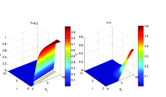
Figure 1: (Color online) Concurrence of the quantum dot vs $k_{0}$ and $r$ for two different $T$.

The concurrences of the quantum dot are ploted in Fig. 1 in terms of the dimensionless quantities $k_{0}$ and $r$, for $T=0.2$ and $T=1$. From Fig. 1 we can see evident differences of the entanglement for the two cases of different temperature. It is the most obvious that the region of entanglement becomes smaller with the rise of temperature. The region of entanglement locates at $r$ smaller, and $k_{0}$ bigger. It is clear that $r$ can restrain the entanglement, however, $k_{0}$ can enhance the entanglement. Moreover, the maximal concurrence of quantum dot becomes smaller at $T=0.2$ than $T=1$. That is to say, the increasing temperature will damage the entanglement of the system.

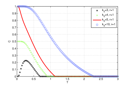
Figure 2: (Color online) Concurrence vs temperature ($T$) for different $k_{0}$ in the case of $r=1$: $k_{0}=4$ (green cross line), $k_{0}=5$ (red solid line), $k_{0}=10$ (blue circle line).

To better illustrate the relation of the concurrence versus temperature, we plot the concurrence as functions of the dimensionless quantities $T$ in the four cases of different $k_{0}$ at fixed $r$ in Fig. 2. This figure show $C$ is a monotonically decreasing function to $T$ with $r\leq\frac{1}{4}k_{0}$, and all the curves eventually approach $C=0$(disentanglement), corresponding to $k_{0}=4,5,10$ and $r=1$. When $r>\frac{1}{4}k_{0}$, the curve will firstly raise from $0$ to a top, then decline, finally decrease $C=0$, corresponding to $k_{0}=3$ and $r=1$. The reason of them will be analyzed in the following. The system lies in the ground state at zero temperature. For $r<\frac{1}{4}k_{0}$, the ground state is $|\Psi_{4}\rangle$, which is the maximally entangled state, so $C=1$ for $T=0$. With increasing the temperature, $|\Psi_{4}\rangle$ will mix with the higher energy levels respectively, namely, $|\Psi_{2}\rangle$, $|\Psi_{3}\rangle$ and $|\Psi_{1}\rangle$, so the concurrence monotonically decreases from $1$ to $0$. However, the ground state become $|\Psi_{2}\rangle$, the disentangled state, in the case of $r>\frac{1}{4}k_{0}$, so $C=0$ for $T=0$. Similar the case, $|\Psi_{2}\rangle$ will mix with $|\Psi_{4}\rangle$, $|\Psi_{3}\rangle$ and $|\Psi_{1}\rangle$. Hence the concurrence firstly increases, then decreases. When $r=\frac{1}{4}k_{0}$, the ground state will be the degenerate state of $|\Psi_{2}\rangle$ and $|\Psi_{4}\rangle$. the probabilities of both state in the ground state are all $50\%$, so $C=0.5$ at $T=0$. These results are all shown in Fig. 2. In addition, the values of the critical $T_{C}$, lead to the system disentanglement $C=0$, can be calculated as

$$T_{C}=\frac{k_{0}}{4ln3}.$$ (23)

It shows the relation $T_{C}$ and $k_{0}$ is linear and monotonic increasing. These result shows that $k_{0}$ can be used as a converter for $T_{C}$, be used to adjust the value of $T_{C}$, namely, change the temperature of turning on or off the entanglement. So $k_{0}$ can be a switch to entanglement, and is tunable, e.g., by means of a external magnetic field $B$ mp ; mpl . For this properties, possible applications are expected in the further.

From the results shown in the above, one may find that $k_{0}$ may enhance the concurrence, but $r$ and $T$ may restrain the entanglement.

IV Quantum teleportation

Quantum teleportation via an arbitrary mixed state was first investigated by G. Bowen and S. Bose gbs . They showed when an arbitrary two-qubit mixed state $\chi$ is used as quantum channel, the depolarizing (or Pauli) channel is given. Recently F. Caruso et al. further generalized it to $N$-qubit fca .

Now we study the quantum teleportation through the quantum dot using the standard teleportation protocol $P_{0}$. Without loss of generality, we consider the input state is an arbitrary pure state of a qubit $|\varphi\rangle_{in}=cos\frac{\theta}{2}|1\rangle+e^{i\phi}sin\frac{\theta}{2}|0\rangle$ ($0\leq\theta\leq\pi,0\leq\phi\leq 2\pi$). So the system of the teleported state and quantum dot in the product state is described by

$$\rho=\rho_{in}\otimes\rho(T),$$ (24)

where $\rho_{in}=|\varphi\rangle_{in}\langle\varphi|$ is the density matrix of the input state. When a joint Bell-basis measurement is performed on the first two spins, the state of the third spin will collapse. Under the projection operators $M_{i}$, $\rho$ yields xxx1

$$\rho_{i}=M_{i}\rho M_{i}^{{\dagger}},$$ (25)

where $M_{i}=E^{i}\otimes I(i=0,1,2,3)$, $E^{0}=|\Psi^{-}\rangle\langle\Psi^{-}|$, $E^{1}=|\Psi^{+}\rangle\langle\Psi^{+}|$, $E^{2}=|\Phi^{-}\rangle\langle\Phi^{-}|$ and $E^{3}=|\Phi^{+}\rangle\langle\Phi^{+}|$, which $|\Psi^{\pm}\rangle=\frac{1}{\sqrt{2}}(|10\rangle\pm|01\rangle)$, $|\Phi^{\pm}\rangle=\frac{1}{\sqrt{2}}(|11\rangle\pm|00\rangle)$. We can see that $E^{0}$ and $E^{1}$ are in the isotropy subspace and $E^{2}$ and $E^{3}$ in the anisotropy subspace. By the tracing over the first two qubits, we can obtain $\rho^{{}^{\prime}}_{i}=\frac{tr_{12}(\rho_{i})}{z}$, which $z=tr(tr_{12}\rho_{i})$. By the tedious calculations, we can obtain the expressions of $\rho^{{}^{\prime}}_{i}$ respectively

$$\rho^{{}^{\prime}}_{1}=\frac{1}{z_{1}}\left(\begin{array}[]{cc}w\cos^{2}\frac{\theta}{2}+u\sin^{2}\frac{\theta}{2}&-\frac{1}{2}y\sin\theta e^{-i\delta}\\ -\frac{1}{2}y\sin\theta e^{i\delta}&v\cos^{2}\frac{\theta}{2}+w\sin^{2}\frac{\theta}{2}\\ \end{array}\right),$$ (28)

$$\rho^{{}^{\prime}}_{2}=\frac{1}{z_{1}}\left(\begin{array}[]{cc}w\cos^{2}\frac{\theta}{2}+u\sin^{2}\frac{\theta}{2}&\frac{1}{2}y\sin\theta e^{-i\delta}\\ \frac{1}{2}y\sin\theta e^{i\delta}&v\cos^{2}\frac{\theta}{2}+w\sin^{2}\frac{\theta}{2}\\ \end{array}\right),$$ (31)

$$\rho^{{}^{\prime}}_{3}=\frac{1}{z_{2}}\left(\begin{array}[]{cc}u\cos^{2}\frac{\theta}{2}+w\sin^{2}\frac{\theta}{2}&-\frac{1}{2}y\sin\theta e^{i\delta}\\ -\frac{1}{2}y\sin\theta e^{-i\delta}&w\cos^{2}\frac{\theta}{2}+v\sin^{2}\frac{\theta}{2}\\ \end{array}\right),$$ (34)

$$\rho^{{}^{\prime}}_{4}=\frac{1}{z_{2}}\left(\begin{array}[]{cc}u\cos^{2}\frac{\theta}{2}+w\sin^{2}\frac{\theta}{2}&\frac{1}{2}y\sin\theta e^{i\delta}\\ \frac{1}{2}y\sin\theta e^{-i\delta}&w\cos^{2}\frac{\theta}{2}+v\sin^{2}\frac{\theta}{2}\\ \end{array}\right),$$ (37)

where $z_{1}=w+u\sin^{2}\frac{\theta}{2}+v\cos^{2}\frac{\theta}{2}$ and $z_{2}=w+v\sin^{2}\frac{\theta}{2}+u\cos^{2}\frac{\theta}{2}$. When the temperature tends to zero, we can note that $\rho^{{}^{\prime}}_{1}$ tends to $\rho_{in}$ arising from $|\Psi_{4}\rangle=|\Psi^{-}\rangle$. So at low temperature, we can obtain the desired teleported state $\rho^{{}^{\prime}}_{1}$ by the $|\Psi^{-}\rangle$ measurement. In the standard protocol, the Pauli rotations $\sigma^{j}(j=z,x,y)$ are respectively applied on $\rho^{{}^{\prime}}_{2}$, $\rho^{{}^{\prime}}_{3}$ and $\rho^{{}^{\prime}}_{4}$. By the Bell-basis measurement in the isotropy and anisotropy subspaces, the output states may be given respectively by

$$\rho^{e}_{out}=\frac{1}{z_{2}}\left(\begin{array}[]{cc}w\cos^{2}\frac{\theta}{2}+v\sin^{2}\frac{\theta}{2}&-\frac{1}{2}y\sin\theta e^{-i\delta}\\ -\frac{1}{2}y\sin\theta e^{i\delta}&u\cos^{2}\frac{\theta}{2}+w\sin^{2}\frac{\theta}{2}\\ \end{array}\right),$$ (41)

$$\rho^{o}_{out}=\rho^{{}^{\prime}}_{1}.$$ (42)

It is worth noting that $\rho^{e}_{out}=\rho^{o}_{out}$ at $r=0$, which is the degenerate point from Eq.(II). The output states corresponding to both different subspaces measurement outcomes have a small difference, which is derived from the magnetic field.

To characterize the quality of the teleported state, the fidelity, as a useful probe, between $|\varphi\rangle_{in}$ and $\rho_{out}$ is defined by

$$F=\;\;_{in}\langle\varphi|\rho_{out}|\varphi\rangle_{in}.$$ (43)

In addition, the average fidelity $F^{a}$ of teleportation can be formulated as

$$F^{a}=\frac{\int^{2\pi}_{0}d\delta\int^{\pi}_{0}F\sin\theta d\theta}{4\pi}.$$ (44)

If quantum dot is used as the quantum channel, making use of Eqs. (43) and (44) we can calculate the expressions of the anisotropy fidelity $F^{o}$, the anisotropy fidelity $F^{e}$ and the average fidelity $F^{a}$.

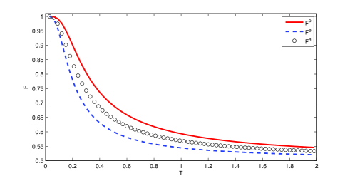
Figure 3: (Color online) The fidelity as a function of temperature $T$ with $k_{0}=2$ and $r=0.2$. $F^{o}$ and $F^{e}$ are plotted for $\theta=\frac{\pi}{3}$.

The fidelity is plotted as a function of temperature $T$ in Fig. 3. The evolution of the fidelity, decrease monotonously, is shown as temperature increases. The evolution curves of $F^{o}$, $F^{e}$ and $F^{a}$ are very similar in shape, but the value of $F^{o}$ is always larger than that of $F^{e}$. The value of $F^{a}$ is in the middle of them. It easily can be seen that three fidelity is equal to one and and quantum teleportation is perfectly achieved at the zero temperature, because $|\Psi_{4}\rangle$ is the ground state and equal to $|\Psi^{-}\rangle$ in the conditions of Fig. 3. However, as $T$ increases, not only the thermal entanglement decay, but also the ground state mix with the excited states, which lead to the fidelity of teleportation decline. Firstly, the fidelity fall rapidly, then changes slowly.

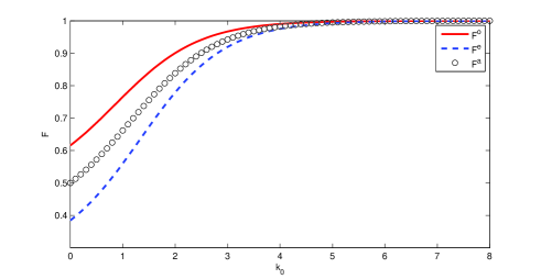
Figure 4: (Color online) The fidelity as a function of $k_{0}$ with $T=0.2$ and $r=0.2$. $F^{o}$ and $F^{e}$ are plotted for $\theta=\frac{\pi}{3}$.

Figure 4 gives the dependence of the fidelity on $k_{0}$ at finite temperature. As $k_{0}$ increases, the upper results show that the entanglement increases. Here the fidelity increase monotonically as $k_{0}$ increases. For the fixed $T=0.2$ and $r=0.2$, the fidelity increases rapidly to one and keep perfectly stable. Therefore, $k_{0}$ is beneficial for the teleportation. Three kinds of the fidelity always are similar in shape and the value of $F^{o}$ is always larger than that of $F^{e}$.

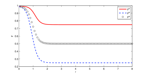
Figure 5: (Color online) The fidelity as a function of $r$ with $T=0.2$ and $k_{0}=4$. $F^{o}$ and $F^{e}$ are plotted for $\theta=\frac{\pi}{3}$.

Figure 5 depicts the effects of $r$ on the fidelity of teleportation. In general, the effect on the quantum teleportation system is found to be similar. They all first decrease rapidly, then tend to stable. It is very obvious that $F^{o}$ is always superior to $F^{e}$. When $r=0$, one can see $F^{o}=F^{e}=F^{a}=1$, which indicates that in this case the quality of the teleportation is perfect. But the introduction of $r$ not only induces them to separate but also causes them to decrease in the standard protocol. In addition, the average fidelity $F^{a}$ tends steadily to $0.5$. These illustrate that quantum dot is a better channel for teleportation. These results show $F^{o}$ is always superior to $F^{e}$, because the eigenstates of the system $|\Psi_{3}\rangle$ and $|\Psi_{4}\rangle$ are just Bell measurements $|\Psi^{+}\rangle$ and $|\Psi^{-}\rangle$ in the anisotropy subspace.

V conclusion

Summarizing, we simplify the Hamiltonian of the quantum dot to the nature Hamiltonian by integrating and finding the unitary matrix. We explored how the important physical quantities affect the thermal entanglement and quantum teleportation. The results show $k_{0}$ can improve the entanglement and the quality of the quantum teleportation. The critical temperature of disentanglement is given. In addition, we obtain the explicit expression of the output state of the teleportation based on Bell measurements, with quantum dot as quantum channel. This allows us to calculate the transmission fidelity of the quantum channel. Based on Bell measurements in two subspaces, we found $F^{o}$ is always optimal to $F^{e}$ due to arising from the eigenstates of the system in the anisotropy subspace. It is shown that the anisotropy transmission fidelity is very high and stable for quantum dot as quantum channel. These possible applications are expected in the quantum teleportation.

VI Acknowledgement

This work is partly supported by the NSF of China (Grant No. 11075101), Shanghai Leading Academic Discipline Project (Project No. S30105), and Shanghai Research Foundation (Grant No. 07d222020). The authors are grateful to Xin-Jian Xu for valuable discussions.

References

- (1) G. Bowen and S. Bose, Phys. Rev. Lett. 87, 267901 (2001).
- (2) S. Bose Phys. Rev. Lett. 91, 207901 (2003).
- (3) I. D. K. Brown, S. Stepney, A. Sudbery, and S. L. Braunstein, J. Phys. A 38, 1119 (2005).
- (4) M. Blasone, F. Dell Anno, S. De Siena, and F. Illuminati, Phys. Rev. A 77, 062304 (2008).
- (5) D. D. B. Rao, S. Ghosh, and P. K. Panigrahi, Phys. Rev. A 78 042328 (2008).
- (6) Y. Yeo, Phys. Rev. A 66, 062312 (2002).
- (7) Y. Yeo, T. Q. Liu, Y. E. Lu, and Q. Z. Yang, J. Phys. A 38, 3235 (2005).
- (8) G. F. Zhang, Phys. Rev. A, 75 034304 (2007).
- (9) Y. Zhou, G. F. Zhang, S. S. Li, and A. Abliz, Europhys. Lett. 86 50004 (2009).
- (10) Y. Zhou, G.F. Zhang, Eur. Phys. J. D, 47 227 (2008).
- (11) J. L. Guo, and H. S. Song, Eur. Phys. J. D, 56 265 (2010).
- (12) F. Kheirandish, S. J. Akhtarshenas, and H. Mohammadi, Phys. Rev. A 77, 042309 (2008).
- (13) S. Albeverio, S.-M. Fei, and W.-L. Yang, Phys. Rev. A 66, 012301 (2002).
- (14) P. Solinas, P. Zanardi, N. Zanghi, and F. Rossi, Phys. Rev. A 67, 052309 (2003).
- (15) E. Lombardi, F. Sciarrino, S. Popescu, and F. De Martini, Phys. Rev. Lett. 88, 070402 (2002); Hai-Wong Lee and J. Kim, Phys. Rev. A 63, 012305 (2001)
- (16) K. W. Choo and L. C. Kwek, Phys. Rev. B 75, 205321 (2007).
- (17) F. de Pasquale, G. Giorgi, and S. Paganelli, Phys. Rev. Lett. 93, 120502 (2004).
- (18) S. Sasaki, S.De Franceschi, J. M. Elzerman, W. G. van der Wiel, M. Eto, S. Tarucha, and L. P. Kouwenhoven, Nature 405, 764 (2000).
- (19) M. Pustilnic, and L. I. Glazman, Phys. Rev. Lett. 85 2993 (2000).
- (20) M. Pustilnic, and L. I. Glazman, Phys. Rev. Lett. 87, 216601 (2001).
- (21) M. Pustilnik and L. I. Glazman, Phys. Rev. B 64, 045328 (2001).
- (22) M. Pustilnik, L. I. Glazman, and W. Hofstetter, Phys. Rev. B 68, 161303 (2003).
- (23) I. L. Kurland, I. L. Aleiner, and B. L. Altshuler, arXiv:cond-mat/0004205v1.
- (24) S. Hill, W. K. Wootters, Phys. Rev. Lett. 78, 5022 (1997); W. K. Wootters, Phys. Rev. Lett. 80, 2245 (1998).
- (25) H. Fu, A. I. Solomon, and X. Wang, J. Phys. A 35, 4293 (2002);
- (26) F. Caruso, V. Giovannetti, and G. M. Palma, Phys. Rev. Lett. 104, 020503 (2010).