Second Order Perturbations During Inflation Beyond Slow-roll

Abstract

We numerically calculate the evolution of second order cosmological perturbations for an inflationary scalar field without resorting to the slow-roll approximation or assuming large scales. In contrast to previous approaches we therefore use the full non-slow-roll source term for the second order Klein-Gordon equation which is valid on all scales. The numerical results are consistent with the ones obtained previously where slow-roll is a good approximation. We investigate the effect of localised features in the scalar field potential which break slow-roll for some portion of the evolution. The numerical package solving the second order Klein-Gordon equation has been released under an open source license and is available for download.

1 Introduction

The arrival of more and better data in the last couple of years has fundamentally changed theoretical cosmology. Until only a few years ago it was sufficient to use linear order theory to analyse the data and calculate first order observables, such as the power spectrum; higher order theory wasn’t required. The new data, in particular the Cosmic Microwave Background (CMB) anisotropy maps as provided by the Wmap and the Planck satellites [1, 2], make it possible to go beyond linear order and derive higher order observables such as the bispectrum from the data. Considerable effort has therefore been spent on extracting observable signatures beyond the power spectrum and to extend cosmological perturbation theory beyond linear order.

So far calculations of higher order observables such as the bispectrum, or its popular parametrisation $f_{\mathrm{NL}}$, have relied heavily on approximations. This meant usually assuming large scales, that is large compared to the “horizon”, and imposing slow-roll [3]. However, these restrictions not only constrain the validity of the results, but also limit the number of models that can be studied, excluding many interesting cases. For example, even in linear theory it is already well known that interesting and observable effects occur when slow-roll is violated at the end of inflation [4].

Second order perturbations play a crucial role in our quest to understand the non-linear physics of the early universe. Previous works by us and collaborators [5, 6] have derived the equations of motion for second order perturbations in the long wavelength approximation, the slow-roll approximation and also the full non-slow-roll case for all scales [7].

Previously in Ref. [8] we numerically solved the evolution of second order perturbations under the assumption that the source term, which consists of convolutions of first order perturbations and their derivatives, is calculated in the slow-roll approximation. We showed that the source term closely follows the form of the first order power spectrum. In this paper we go beyond the slow roll approximation to calculate the full source term equations for a single scalar field. This full treatment is needed in cases where slow-roll is broken. The results of the updated calculation are consistent with those of our previous work for the $\frac{1}{2}m^{2}\varphi^{2}$ potential for which the slow-roll approximation is an exceptionally good one. To go beyond slow-roll in this paper, we study “step” and “bump” potentials, for which slow-roll is broken as $|\eta_{V}|>1$ around the feature ($\eta_{V}$ denoting one of the slow-roll parameters). Step potentials have been widely used to create features in the power spectrum of inflationary perturbations which might more accurately match the observed power spectrum from WMAP [9, 10, 11, 12, 13, 14]. In this paper we will follow the potential forms described by Chen et al. [15, 16]. In addition to being able to calculate the second order field perturbation in this case, the result of the full equations seems to be smoother at very early times when the perturbations are highly oscillatory (due to a larger damping term, which is lost in slow-roll).

The final goal of this continuing work is a numerical calculation of the curvature perturbation at second order for all length scales. This will probe effects both inside and outside the horizon in a way that is not possible using other methods, for example the $\delta N$ formalism [17, 18, 19, 20, 21], which a priori uses large scales only. The applications of such a calculation are many and varied and range from an investigation of the non-Gaussian nature of inflationary perturbations to the exploration of higher order effects such as the sourcing of gravitational waves at second order [22] and vorticity generation [23].

In the current paper we have only considered the effect of a single scalar field. One goal of future work is to extend the numerical code to deal with more than one field. In a multifield system the curvature perturbation is not the only important observable with isocurvature components also playing a significant role. Calculating the field evolution is the only way to gain access to these isocurvature results, in a way that would not be possible if we had concentrated purely on the curvature perturbations. With this goal in mind we have fashioned the numerical calculation in terms of a scalar field instead of the curvature perturbation which might otherwise have been considered a more observationally relevant quantity in the single field case. We have developed the numerical code considerably from that used in Ref. [8]. The change from the slow-roll to full equations adds significant complexity to the calculation but this has been countered by optimising the time sensitive functions and implementing more of them in a compiled language. The numerical code has been released under an open source license (Modified BSD license) and is available for download [24].

In Section 2 we present the Klein-Gordon equation for second order cosmological perturbations. This is the central part of the code described in Section 3. The results we have obtained are in Section 4 and discussion of these and future goals is contained in Section 5. Throughout the text we use $8\pi G$ and label conformal time derivatives with a prime. We assume a flat Friedmann-Robertson-Walker background throughout this paper.

2 Second Order Perturbations

2.1 Klein Gordon Equations

Cosmological perturbations beyond linear order have been studied in depth in recent times and a brief summary can be found in Appendix A or at length in Refs. [25, 26] (see Ref. [27] for an example of earlier work in this area). In particular the Klein-Gordon equations for the background, first order and second order perturbations are given in Eqs. (A.15)-(A). These equations are given in real space, however, and in general the dynamics of the scalar field become clearer in Fourier space. Following Refs. [3] and [7] we will write $\delta\varphi(k^{i})$ for the Fourier component of $\delta\varphi(x^{i})$ such that

$$\delta\varphi(\eta,x^{i})=\frac{1}{(2\pi)^{3}}\int\mathrm{d}^{3}k\delta\varphi(k^{i})\exp(ik_{i}x^{i})\,,$$ (2.1)

where $k^{i}$ is the comoving wavenumber. In Fourier space, the closed form of the first order Klein-Gordon equation (A.16) then transforms into

$$\delta\varphi_{1}(k^{i})^{\prime\prime}+2\mathcal{H}\delta\varphi_{1}(k^{i})^{\prime}+k^{2}\delta\varphi_{1}(k^{i})\\ +a^{2}\left[V_{,\varphi\varphi}+\frac{8\pi G}{\mathcal{H}}\left(2\varphi_{0}^{\prime}V_{,\varphi}+(\varphi_{0}^{\prime})^{2}\frac{8\pi G}{\mathcal{H}}V_{0}\right)\right]\delta\varphi_{1}(k^{i})=0\,,$$ (2.2)

where $\varphi_{0}$ is the background homogeneous scalar field, $\delta\varphi_{1}$ is the first order scalar field perturbation, $a$ is the FRW scale factor, $\mathcal{H}=a^{\prime}/a$ is the conformal Hubble parameter and $V$ is the potential of the scalar field with derivatives w.r.t $\varphi$ denoted by $V_{,\varphi}$ etc. The second order equation (A) requires a careful consideration of terms that are quadratic in the first order perturbation. Terms at second order of the form $\left(\delta\varphi_{1}(x^{i})\right)^{2}$ require the use of the convolution theorem (see for example Ref. [28]). We use convolutions of the form

$$f(x^{i})g(x^{i})\longrightarrow\frac{1}{(2\pi)^{3}}\int\mathrm{d}^{3}q\mathrm{d}^{3}p\,\delta^{3}(k^{i}-p^{i}-q^{i})f(p^{i})g(q^{i})\,.$$ (2.3)

The full closed form, second order Klein-Gordon equation in Fourier space is then given by [7]

$$\delta\varphi_{2}^{\prime\prime}(k^{i}) +2\mathcal{H}\delta\varphi_{2}^{\prime}(k^{i})+k^{2}\delta\varphi_{2}(k^{i})$$

$$+a^{2}\left[V_{,\varphi\varphi}+\frac{8\pi G}{\mathcal{H}}\left(2\varphi_{0}^{\prime}V_{,\varphi}+(\varphi_{0}^{\prime})^{2}\frac{8\pi G}{\mathcal{H}}V_{0}\right)\right]\delta\varphi_{2}(k^{i})$$

$$+S(k^{i})=0\,.$$ (2.4)

The source term $S$ contains all the products of $\delta\varphi_{1}$ in real space which require convolution integrals. Terms which contain gradients of $\delta\varphi_{1}$ include additional factors of $k$ and $q$. The form of $S$ is given by [7]

$$S\left(\delta\varphi_{1}(k^{i}),\delta\varphi_{1}^{\prime}(k^{i})\right)=\frac{1}{(2\pi)^{3}}\int\mathrm{d}^{3}p\,\mathrm{d}^{3}q\,\delta^{3}(k^{i}-p^{i}-q^{i})\Bigg{\{}$$

$$\quad 2\frac{8\pi G}{\mathcal{H}}\left[Q\delta\varphi_{1}^{\prime}(p^{i})\delta\varphi_{1}(q^{i})+\varphi_{0}^{\prime}a^{2}V_{,\varphi\varphi}\delta\varphi_{1}(p^{i})\delta\varphi_{1}(q^{i})\right]$$

$$\quad+\left(\frac{8\pi G}{\mathcal{H}}\right)^{2}\varphi_{0}^{\prime}\left[2a^{2}V_{,\varphi}\varphi_{0}^{\prime}\delta\varphi_{1}(p^{i})\delta\varphi_{1}(q^{i})+\varphi_{0}^{\prime}Q\delta\varphi_{1}(p^{i})\delta\varphi_{1}(q^{i})\right]$$

$$\quad-2\left(\frac{8\pi G}{2\mathcal{H}}\right)^{2}\frac{\varphi_{0}^{\prime}Q}{\mathcal{H}}\left[Q\delta\varphi_{1}(p^{i})\delta\varphi_{1}(q^{i})+\varphi_{0}^{\prime}\delta\varphi_{1}(p^{i})\delta\varphi_{1}^{\prime}(q^{i})\right]$$

. $$\quad+\frac{8\pi G}{2\mathcal{H}}\varphi_{0}^{\prime}\delta\varphi_{1}^{\prime}(p^{i})\delta\varphi_{1}^{\prime}(q^{i})+a^{2}\left[V_{,\varphi\varphi\varphi}+\frac{8\pi G}{\mathcal{H}}\varphi_{0}^{\prime}V_{,\varphi\varphi}\right]\delta\varphi_{1}(p^{i})\delta\varphi_{1}(q^{i})$$

$$\quad+2\left(\frac{8\pi G}{\mathcal{H}}\right)\frac{p_{k}q^{k}}{q^{2}}\delta\varphi_{1}^{\prime}(p^{i})\left(Q\delta\varphi_{1}(q^{i})+\varphi_{0}^{\prime}\delta\varphi_{1}^{\prime}(q^{i})\right)+p^{2}2\frac{8\pi G}{\mathcal{H}}\delta\varphi_{1}(p^{i})\varphi_{0}^{\prime}\delta\varphi_{1}(q^{i})$$

$$\quad+\left(\frac{8\pi G}{2\mathcal{H}}\right)^{2}\frac{\varphi_{0}^{\prime}}{\mathcal{H}}\Bigg{[}\left(p_{l}q^{l}-\frac{p^{i}q_{j}k^{j}k_{i}}{k^{2}}\right)\varphi_{0}^{\prime}\delta\varphi_{1}(p^{i})\varphi_{0}^{\prime}\delta\varphi_{1}(q^{i})\Bigg{]}$$

$$\quad+2\frac{Q}{\mathcal{H}}\left(\frac{8\pi G}{2\mathcal{H}}\right)^{2}\frac{p_{l}q^{l}p_{m}q^{m}+p^{2}q^{2}}{k^{2}q^{2}}\Bigg{[}\varphi_{0}^{\prime}\delta\varphi_{1}(p^{i})\left(Q\delta\varphi_{1}(q^{i})+\varphi_{0}^{\prime}\delta\varphi_{1}^{\prime}(q^{i})\right)\Bigg{]}$$

$$\quad+\frac{8\pi G}{2\mathcal{H}}\Bigg{[}4Q\frac{q^{2}+p_{l}q^{l}}{k^{2}}\left(\delta\varphi_{1}^{\prime}(p^{i})\delta\varphi_{1}(q^{i})\right)-\varphi_{0}^{\prime}p_{l}q^{l}\delta\varphi_{1}(p^{i})\delta\varphi_{1}(q^{i})\Bigg{]}$$

$$\quad+\left(\frac{8\pi G}{2\mathcal{H}}\right)^{2}\frac{\varphi_{0}^{\prime}}{\mathcal{H}}\Bigg{[}\frac{p_{l}q^{l}p_{m}q^{m}}{p^{2}q^{2}}\left(Q\delta\varphi_{1}(p^{i})+\varphi_{0}^{\prime}\delta\varphi_{1}^{\prime}(p^{i})\right)\left(Q\delta\varphi_{1}(q^{i})+\varphi_{0}^{\prime}\delta\varphi_{1}^{\prime}(q^{i})\right)\Bigg{]}$$

$$\quad+\frac{\varphi_{0}^{\prime}}{\mathcal{H}}\Bigg{[}8\pi G\left(\frac{p_{l}q^{l}+p^{2}}{k^{2}}q^{2}\delta\varphi_{1}(p^{i})\delta\varphi_{1}(q^{i})-\frac{q^{2}+p_{l}q^{l}}{k^{2}}\delta\varphi_{1}^{\prime}(p^{i})\delta\varphi_{1}^{\prime}(q^{i})\right)$$

$$\quad+\left(\frac{8\pi G}{2\mathcal{H}}\right)^{2}\frac{k^{j}k_{i}}{k^{2}}\Bigg{(}2\frac{p^{i}p_{j}}{p^{2}}\left(Q\delta\varphi_{1}(p^{i})+\varphi_{0}^{\prime}\delta\varphi_{1}^{\prime}(p^{i})\right)Q\delta\varphi_{1}(q^{i})\Bigg{)}\Bigg{]}\Bigg{\}}\,,$$ (2.5)

where we have defined the parameter $Q=a^{2}(8\pi GV_{0}\varphi_{0}^{\prime}/\mathcal{H}+V_{,\varphi})$ for convenience. Calculating Eq. (2.1) is the main task of the numerical simulation described in Section 3.

2.2 Equations for Numerical Calculation

In the previous section the governing equations of the second order system were given in terms of conformal time. A more appropriate time variable for the numerical simulation is the number of e-foldings, $\mathcal{N}=\log(a/a_{\mathrm{init}})$. This is measured from $a_{\mathrm{init}}$, the value of $a$ at the beginning of the simulation. We take the value of the scale factor today, $a_{0}$, as $a_{0}=1$ and calculate $a$ at the end of inflation by connecting it with $a_{0}$ (see discussion in Ref. [29] or for example Eq. (3.19) in Ref. [3]). We also assume that reheating was instantaneous at the end of inflation. We will use a dagger (^†) to denote differentiation with respect to $\mathcal{N}$. Derivatives with respect to conformal time, $\eta$, and coordinate time, $t$, are then given by

$$\frac{\partial}{\partial\eta} =\frac{\mathrm{d}\mathcal{N}}{\mathrm{d}\eta}\frac{\partial}{\partial\mathcal{N}}=\mathcal{H}\frac{\partial}{\partial\mathcal{N}}\,,$$ (2.6)

$$\frac{\partial}{\partial t} =\frac{\mathrm{d}\eta}{\mathrm{d}t}\frac{\mathrm{d}\mathcal{N}}{\mathrm{d}\eta}\frac{\partial}{\partial\mathcal{N}}=H\frac{\partial}{\partial\mathcal{N}}\,,$$ (2.7)

respectively, where $H=\mathrm{d}\ln a/\mathrm{d}t$ and $\mathcal{H}=aH$. The background and first order equations, written in terms of the new time variable $\mathcal{N}$, are

$$\varphi_{0}^{\dagger\dagger}+\left(3+\frac{H^{\dagger}}{H}\right)\varphi_{0}^{\dagger}+\frac{V_{,\varphi}}{H^{2}}=0\,,$$ (2.8)

and

$$\delta\varphi_{1}^{\dagger\dagger}(k^{i})+\left(3+\frac{H^{\dagger}}{H}\right)\delta\varphi_{1}^{\dagger}(k^{i})+\Bigg{[}\left(\frac{k}{aH}\right)^{2}+\frac{V_{,\varphi\varphi}}{H^{2}}+\frac{8\pi G}{H^{2}}2\varphi_{0}^{\dagger}V_{,\varphi}\\ +\left.\left(\frac{8\pi G}{H}\right)^{2}\left(\varphi_{0}^{\dagger}\right)^{2}V_{0}\right]\delta\varphi_{1}(k^{i})=0\,.$$ (2.9)

The three-dimensional convolution integral $\int\mathrm{d}q^{3}$ can be rewritten in spherical coordinates $q,\theta,\omega$ where $q=|q^{i}|$. There is no $\omega$ dependence in the source term integral but $|k^{i}-q^{i}|$ and the factors of $k^{i}$ and $q^{i}$ are dependent on $\theta$ and this dependence is made explicit below. Eqs. (2.1) and (2.1) must be written in terms of $\mathcal{N}$, with the $\theta$ dependent terms grouped together, in order to set up the numerical system completely at second order. In the slow-roll case there were only four different $\theta$ dependent terms, here labelled $\mathcal{A}$–$\mathcal{D}$ following Ref. [8]:

$$\mathcal{A}(k^{i},q^{i}) =\int_{0}^{\pi}\sin(\theta)\delta\varphi_{1}(k^{i}-q^{i})\mathrm{d}\theta\,,$$

$$\mathcal{B}(k^{i},q^{i}) =\int_{0}^{\pi}\cos(\theta)\sin(\theta)\delta\varphi_{1}(k^{i}-q^{i})\mathrm{d}\theta\,,$$

$$\mathcal{C}(k^{i},q^{i}) =\int_{0}^{\pi}\sin(\theta)\delta\varphi_{1}^{\dagger}(k^{i}-q^{i})\mathrm{d}\theta\,,$$

$$\mathcal{D}(k^{i},q^{i}) =\int_{0}^{\pi}\cos(\theta)\sin(\theta)\delta\varphi_{1}^{\dagger}(k^{i}-q^{i})\mathrm{d}\theta\,.$$ (2.10)

The non-slow-roll source term in Eq. (2.2) that we are now considering requires the use of three further $\theta$ integrals in addition to those in Eq. (2.2), which are

$$\mathcal{E}(k^{i},q^{i}) =\int_{0}^{\pi}\cos^{2}(\theta)\sin(\theta)\delta\varphi_{1}(k^{i}-q^{i})\mathrm{d}\theta\,,$$

$$\mathcal{F}(k^{i},q^{i}) =\int_{0}^{\pi}\frac{\sin^{3}(\theta)}{|k^{i}-q^{i}|^{2}}\delta\varphi_{1}(k^{i}-q^{i})\mathrm{d}\theta\,,$$

$$\mathcal{G}(k^{i},q^{i}) =\int_{0}^{\pi}\frac{\sin^{3}(\theta)}{|k^{i}-q^{i}|^{2}}\delta\varphi_{1}^{\dagger}(k^{i}-q^{i})\mathrm{d}\theta\,.$$ (2.11)

It is worth noting that the term $\sin^{3}(\theta)/|k^{i}-q^{i}|^{2}$ tends to zero in the limit where $k=q$ and $\theta\rightarrow 0$. The second order Klein-Gordon equation in e-folding time is

$$\delta\varphi_{2}^{\dagger\dagger}(k^{i})+\left(3+\frac{H^{\dagger}}{H}\right)\delta\varphi_{2}^{\dagger}(k^{i})+\left(\frac{k}{aH}\right)^{2}\delta\varphi_{2}(k^{i})\\ +\frac{1}{H^{2}}\left[V_{,\varphi\varphi}+8\pi G\left(2\varphi_{0}^{\dagger}V_{,\varphi}+8\pi G\left(\varphi_{0}^{\dagger}\right)^{2}V_{0}\right)\right]\delta\varphi_{2}(k^{i})+S(k^{i})=0\,,$$ (2.12)

where the full source equation is given by

$$S(k^{i})= \frac{1}{(2\pi)^{2}}\int\mathrm{d}qq^{2}\Bigg{\{}\frac{1}{\left(H\right)^{2}}\left[V_{,\varphi\varphi\varphi}+3(8\pi G)\varphi_{0}^{\dagger}V_{,\varphi\varphi}\right]\delta\varphi_{1}(q^{i})\mathcal{A}(k^{i},q^{i})$$

$$+\frac{(8\pi G)^{2}\varphi_{0}^{\dagger}}{(aH)^{2}}\left[2a^{2}\varphi_{0}^{\dagger}V_{,\varphi}+Q\left(\varphi_{0}^{\dagger}-\frac{Q}{2(aH)^{2}}\right)\right]\delta\varphi_{1}(q^{i})\mathcal{A}(k^{i},q^{i})$$

$$-\frac{(8\pi G)^{2}}{(aH)^{2}}\frac{(\varphi_{0}^{\dagger})^{2}Q}{2}\delta\varphi_{1}^{\dagger}(q^{i})\mathcal{A}(k^{i},q^{i})$$

$$+\frac{2(8\pi G)Q}{(aH)^{2}}\delta\varphi_{1}(q^{i})\mathcal{C}(k^{i},q^{i})+\frac{8\pi G\varphi_{0}^{\dagger}}{2}\delta\varphi_{1}^{\dagger}(q^{i})\mathcal{C}(k^{i},q^{i})$$

$$+\frac{8\pi G}{(aH)^{2}}\Bigg{\{}\varphi_{0}^{\dagger}\Bigg{[}\left(2k^{2}+\left(\frac{7}{2}-\frac{8\pi G}{4}(\varphi_{0}^{\dagger})^{2}\right)q^{2}+\frac{3}{4}\frac{8\pi G}{(aH)^{2}}Q^{2}\right)\delta\varphi_{1}(q^{i})$$

$$\qquad+(8\pi G)Q\varphi_{0}^{\dagger}\left(\frac{3}{4}+\frac{q^{2}}{k^{2}}\right)\delta\varphi_{1}^{\dagger}(q^{i})\Bigg{]}\mathcal{A}(k^{i},q^{i})$$

$$+\Bigg{[}\left(2Q\frac{q}{k}\left(1-\frac{8\pi G}{(aH)^{2}}Q\varphi_{0}^{\dagger}\right)-\frac{9}{2}\varphi_{0}^{\dagger}kq-\varphi_{0}^{\dagger}\frac{q^{3}}{k}\right)\delta\varphi_{1}(q^{i})$$

$$\qquad-2Q(8\pi G)(\varphi_{0}^{\dagger})^{2}\frac{q}{k}\delta\varphi_{1}^{\dagger}(q^{i})\Bigg{]}\mathcal{B}(k^{i},q^{i})$$

$$+\Bigg{[}\left(-2+(8\pi G)(\varphi_{0}^{\dagger})^{2}\left(\frac{1}{4}+\frac{1}{2aH}\right)\right)Q\delta\varphi_{1}(q^{i})$$

$$\qquad+\left(\frac{8\pi G}{4}(\varphi_{0}^{\dagger})^{2}-2\right)\varphi_{0}^{\dagger}(aH)^{2}\delta\varphi_{1}^{\dagger}(q^{i})\Bigg{]}\mathcal{C}(k^{i},q^{i})$$

$$+\Bigg{[}2Q\frac{k}{q}\delta\varphi_{1}(q^{i})+\left(2\frac{k}{q}-\frac{q}{k}\right)\varphi_{0}^{\dagger}(aH)^{2}\delta\varphi_{1}^{\dagger}(q^{i})\Bigg{]}\mathcal{D}(k^{i},q^{i})$$

$$+(8\pi G)\varphi_{0}^{\dagger}\Bigg{[}\left(\frac{1}{4}(\varphi_{0}^{\dagger})^{2}q^{2}+\frac{Q^{2}}{2(aH)^{2}}\right)\delta\varphi_{1}(q^{i})+\frac{Q}{2}\varphi_{0}^{\dagger}\delta\varphi_{1}^{\dagger}(q^{i})\Bigg{]}\mathcal{E}(k^{i},q^{i})$$

$$+(8\pi G)^{2}\varphi_{0}^{\dagger}Q\Bigg{[}-\frac{Q}{2(aH)^{2}}\left(\frac{k^{2}}{2}+q^{2}\right)\delta\varphi_{1}(q^{i})-\frac{1}{4}\varphi_{0}^{\dagger}k^{2}\delta\varphi_{1}^{\dagger}(q^{i})\Bigg{]}\mathcal{F}(k^{i},q^{i})$$

$$+(8\pi G)^{2}(\varphi_{0}^{\dagger})^{2}\Bigg{[}-\frac{Q}{2}\left(\frac{k^{2}}{2}+\frac{q^{2}}{aH}\right)\delta\varphi_{1}(q^{i})-\frac{(aH)^{2}}{4}\varphi_{0}^{\dagger}k^{2}\delta\varphi_{1}^{\dagger}(q^{i})\Bigg{]}\mathcal{G}(k^{i},q^{i})\Bigg{\}}\Bigg{\}}\,.$$ (2.13)

For comparison, the slow-roll expression for the source term is [8]

$$S(k^{i})=\frac{1}{(2\pi)^{2}}\int\mathrm{d}q\ \Bigg{\{}\frac{V_{,\varphi\varphi\varphi}}{H^{2}}q^{2}\delta\varphi_{1}(q^{i})\mathcal{A}(k^{i},q^{i})$$

$$+\,\frac{8\pi G}{(aH)^{2}}\varphi_{0}^{\dagger}\Bigg{[}\left(3a^{2}V_{,\varphi\varphi}q^{2}+\frac{7}{2}q^{4}+2k^{2}q^{2}\right)\mathcal{A}(k^{i},q^{i})$$

$$-\left(\frac{9}{2}+\frac{q^{2}}{k^{2}}\right)kq^{3}\mathcal{B}(k^{i},q^{i})\Bigg{]}\delta\varphi_{1}(q^{i})$$

$$+\,8\pi G\varphi_{0}^{\dagger}\Bigg{[}-\frac{3}{2}q^{2}\mathcal{C}(k^{i},q^{i})+\left(2-\frac{q^{2}}{k^{2}}\right)kq\mathcal{D}(k^{i},q^{i})\Bigg{]}\delta\varphi_{1}^{\dagger}(q^{i})\Bigg{\}}\,.$$ (2.14)

The increased length of calculation in going from the slow-roll source term in Eq. (2.2) to the full version in Eq. (2.2) can be clearly seen. The numerical complexity is not significantly greater, however, once the three terms in Eq. (2.2) have been calculated. In the next section the implementation of the numerical scheme to calculate the source term in Eq. (2.2) and solve the second order Klein-Gordon equation is discussed.

3 Code Implementation

We described in Ref. [8] a numerical system which calculated the slow-roll source term as given in Eq. (2.2). We have improved the system and the full source term calculation has been implemented. This code has now been released under an open source license [24]. The basic structure of the system is still the same as outlined in Ref. [8] and follows the form laid down by Ref. [30, 31, 32]. Firstly the background fields are evolved to pinpoint the end of inflation when $\epsilon_{H}=-H^{\dagger}/H=1$. The first order Klein-Gordon equation (2.9) is solved using a fourth order Runge-Kutta scheme with the initial conditions specified by the Bunch-Davies vacuum Eq. (3.1). Following this first order stage the source term is calculated at all necessary timesteps. In the last stage of the numerical calculation, the source term result is used to evolve the second order perturbation modes using Eq. (2.12).

The major advance reported in this paper is the use of the full (non-slow-roll) source equation in the third step above. With this advance, seven different terms need to be calculated at each time step. These vary in $k,q$ and $\theta$ and integrals over $q$ and $\theta$ are performed, again at each time step, for each $k$ value. In order to perform these integrals we implement cutoffs at large and small values of $k$. These cutoffs and the integration calculations in general are described in detail in Refs. [8, 29] and we do not discuss them further here. The seven different terms are functional forms of $\theta$ given in Eqs. (2.2) and (2.2). As the first order results are tabulated at specific $k$ values, it is necessary to interpolate the results for $k$ values between these points. The increased complexity of the source equation clearly increases the number of calculations at each time step and hence the overall execution time. The original slow-roll calculation was numerically intensive so the effect of almost doubling the number of calculations could have been dramatic. In fact, optimisation of the code and the translation of some parts into compiled modules has made the increase in complexity manageable. By selecting only particular modes of interest, for example the WMAP pivot scale $k_{\mathrm{WMAP}}=0.002\mathrm{Mpc}^{-1}=5.25\times 10^{-60}M_{\mathrm{PL}}$, the source term calculation can be significantly shortened.

In order to solve the ODEs given in Eqs. (2.8), (2.9) and (2.12) initial values of $\varphi_{0},\delta\varphi_{1},\delta\varphi_{2}$ and their first derivatives must be specified. For the background field initial values of $\varphi_{0}$ and $\varphi_{0}^{\dagger}$ are chosen so that the inflationary period lasts approximately 60 e-foldings after the scales of interest in the CMB exit the horizon. In the case of the quadratic potential this requires choosing super-Planckian initial field values, for example $\varphi_{0,\mathrm{init}}=18M_{\mathrm{PL}}$.

The first order perturbation initial conditions are chosen by assuming that sufficiently far inside the horizon the perturbation modes are in the Bunch-Davies vacuum state. To implement this early time condition in the numerical system we follow Salopek et al. [30] who initialise the first order modes at a time when $k/aH$ for the mode equals some arbitrary factor. In keeping with Ref. [30] we choose this factor to be $50$. The first order initial values are then calculated as

$$\delta\varphi_{1}|_{\mathrm{init}} =\frac{\sqrt{8\pi G}}{a}\frac{e^{-ik\eta}}{\sqrt{2k}}\,,$$ (3.1)

$$\delta\varphi_{1}^{\dagger}|_{\mathrm{init}} =-\frac{\sqrt{8\pi G}}{a}\frac{e^{-ik\eta}}{\sqrt{2k}}\left(1+i\frac{k}{aH}\right)\,,$$ (3.2)

where $\eta$ is the conformal time again.

The situation of the second order initial conditions is different. At the initial times when the Bunch-Davies conditions are suitable the perturbations are expected to be highly Gaussian. In this paper we are interested in the production of second order effects by the evolution of the first order modes and we make no assumptions about the existence of second order perturbations before the simulation begins. Therefore, we set the initial condition for each second order perturbation mode to be $\delta\varphi_{2}=0$, and $\delta\varphi_{2}^{\dagger}=0$ at the time when the corresponding first order perturbation is initialised.

A numerical solution for the second order perturbation equation will contain a homogeneous solution and a particular solution. As stated above we have chosen the initial values for the second order field to be zero. On their own these initial conditions do not remove this homogeneous solution from the result for $\delta\varphi_{2}$ in general. In order to do this, and keep only the particular solution to the equation, it is necessary to ensure that the homogeneous solution is the trivial $(0,0)$ solution throughout the evolution.

In order to only report the particular solution of the second order differential equation Eq. (2.12) we have added a ramping term to the source term $S$. This ramp interpolates between $0$ and $1$ for about an e-folding of time around the time of the initialisation of the modes. By starting the solution of $\delta\varphi_{2},\delta\varphi_{2}^{\dagger}$ at $0,0$ and setting the source term to $0$ at this time through the use of the ramp, the solution for $\delta\varphi_{2}$ will consist only of the inhomogeneous part. The homogeneous solution of Eq. (2.12) i.e., the solution without the source term present, is the same form as the solution for $\delta\varphi_{1}$ as can been seen by comparing Eqs. (2.12) and (2.9). Figure 1 shows the effect that incorporating the ramp has on the source term at early times for the $k_{\mathrm{WMAP}}$ mode. The value of $\delta\varphi_{2}(k_{\mathrm{WMAP}})$ is initialised to be equal to zero at 64.3 e-foldings before the end of inflation, when the ramp value is still zero. The ramp is added to the source term for each mode at the respective initialisation time and all the results below were generated using a ramped source term.

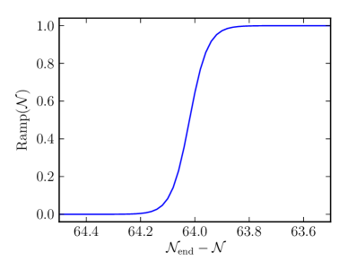
(a) The ramp function used to remove the homogeneous solution for $\delta\varphi_{2}$, here shown around the initialisation time for the scale $k_{\mathrm{WMAP}}$.

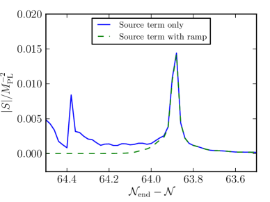
(b) The addition of the ramp term to $S$ changes its value at the initialisation time from the original value (blue solid line) to the ramped value (green dashed line), here shown for scale $k_{\mathrm{WMAP}}$.

Figure 1: The ramping function used with the source term results.

4 Results

4.1 Comparison with Slow-Roll Results

The full second order code has been run with a number of different potentials. Firstly in order to check the consistency of the full equation, the standard slow-roll quadratic potential was used. Figure 2a shows that the results of the full system are very similar to the slow-roll results, as expected for this potential. The additional terms in the source equation Eq. (2.2) subdue some of the oscillatory noise evident in the slow-roll solution at early times when the mode is inside the horizon.

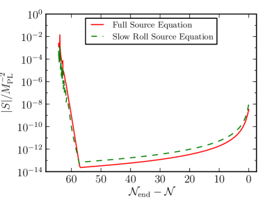
(a) The source term results at all time steps

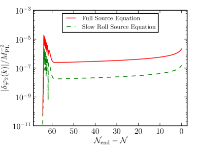
(b) The second order results around the feature

Figure 2: A comparison of the results from the full equations (red solid line) and the slow-roll source term (green dashed line) for scale $k_{\mathrm{WMAP}}$.

The second order result is similar in both cases, however there is an appreciable increase in the amplitude of the second order modes when the full equations are used. This is likely to be a result of the reduced oscillations mentioned above. The second order values are plotted in Figure 2b.

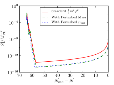
(a) The source term results for the perturbed models

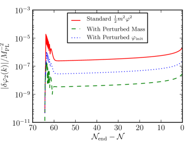
(b) The second order perturbations for the perturbed models

Figure 3: The source term and second order results for models with slightly perturbed mass (green dashed line) and $\varphi_{\mathrm{init}}$ (blue dotted line) compared to the standard quadratic model (red solid line) for scale $k_{\mathrm{WMAP}}$.

The results for background and first order perturbations are robust under small deviations in the initial conditions or the mass parameter in the potential. However, the source term and second order results are not so robust, with any slight variation in the initial value of $\varphi_{0}$ or the mass parameter translating to sizable changes in the magnitude of the results. For example, a small change in the initial field value of $\Delta\varphi_{0,\mathrm{init}}=0.01M_{\mathrm{PL}}$ or in the mass of the inflaton of $\Delta m=1\times 10^{-11}M_{\mathrm{PL}}$ leads to large differences in the source term and second order results and Figure 3 shows the effects of these changes.

4.2 Step and Bump Potentials

Beyond the standard quadratic model, a more interesting potential to consider is one with a feature at a particular scalar field value [9]. Following Chen et al. [15, 16] we have used both a step and a bump potential. The step potential is a modified $\frac{1}{2}m^{2}\varphi^{2}$ potential of the form

$$V_{\rm{s}}(\varphi)=\frac{1}{2}m^{2}\varphi^{2}\left[1+c\left(\tanh\left(\frac{\varphi-\varphi_{\rm{s}}}{d}\right)-1\right)\right]\,,$$ (4.1)

and the bump potential is given by

$$V_{\rm{b}}(\varphi)=\frac{1}{2}m^{2}\varphi^{2}\left[1+c\operatorname{sech}\left(\frac{\varphi-\varphi_{\rm{b}}}{d}\right)\right]\,,$$ (4.2)

where the parameters $c,d,\varphi_{\rm{s}}$ and $\varphi_{\rm{b}}$ control the height, width and central point of the feature respectively. The step potential used here has an extra $(-1)$ term compared to the one used in Ref. [15]. This extra term ensures that $V_{\rm{s}}\rightarrow\frac{1}{2}m^{2}\varphi^{2}$ at early times instead of beginning with a greater amplitude than the standard quadratic potential and only equalling the quadratic value exactly at the feature point. The evolution of the Hubble parameter $H$ is different for both the bump and step potentials compared to the quadratic potential. This changes the value of $a$ at the end of inflation and therefore the value $a_{\mathrm{init}}$ used at the start of the run. In order to compare models with similar initial conditions the following results are for runs where $a_{\mathrm{init}}$ has been made equal in each case. In physical terms this amounts to small redefinitions of the value of $a$ today away from unity, or the consideration of slightly different physical scales today. Due to the strong dependence on initial conditions as shown above, comparison of numerical results is better facilitated by this fixing of $a_{\mathrm{init}}$ than comparing models with different values of $a_{\mathrm{init}}$.

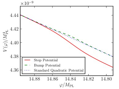
(a) The potential $V(\varphi)$ for the step, bump and standard quadratic potentials around the feature.

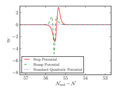
(b) The slow-roll parameter $\eta_{V}$ for the step, bump and quadratic potentials.

Figure 4: The potential and $\eta_{V}$ slow-roll parameter for the step (red solid line), bump (green dashed line) and quadratic (blue dotted line) potentials.

	Step	Bump
$c$	0.0018	0.0005
$d$	0.022	0.01
$\varphi_{\rm{s,b}}$	14.84 $M_{\mathrm{PL}}$	14.84 $M_{\mathrm{PL}}$

Table 1: The values of the parameters in the step and bump potentials.

Figure 4a shows the step and bump potentials at the relevant $\varphi$ values. The features are quite shallow for this choice of parameters but can be tuned to be stronger. The values used in the code are given in Table 1. With these values the slow-roll approximation is temporarily violated as $|\eta|$ gets large around the feature as shown in Figure 4b. We have run the step potential model with a “full” step, corresponding to $c=0.0018$, a “half” step with $c=0.0009$ and finally with $c$ set equal to zero. As a “sanity check” the $c=0$ run gives back the same results as the standard quadratic potential with no feature. The bump potential model has also been run with a “full” bump for which $c=0.0005$, a “half” bump with $c=0.00025$ and a “zero” bump.

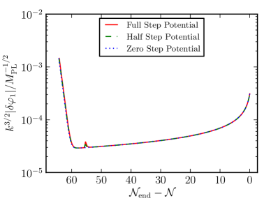
(a) The first order results at all time steps

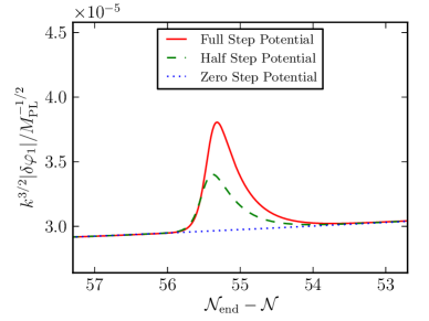
(b) The first order results around the feature

Figure 5: The first order results for the full (red solid line), half (green dashed line) and zero (blue dotted line) step potentials for scale $k_{\mathrm{WMAP}}$.

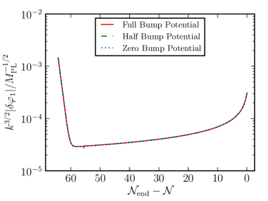
(a) The first order results at all time steps

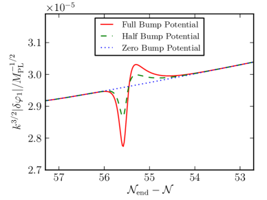
(b) The first order results around the feature

Figure 6: The first order results for the full (red solid line), half (green dashed line) and zero (blue dotted line) bump potentials for scale $k_{\mathrm{WMAP}}$.

The first order spectrum for the three cases for the step potential is plotted in Figure 5 and the cases for the bump potential in Figure 6. At first order the effect of the feature in both potentials is localised around a particular $\varphi$ value and therefore $\mathcal{N}$ value. The half step and bump deviations are smaller than the full ones, however the ratio of the amplitude changes are not symmetric around the central point of the feature. In the source term calculation the presence of a feature makes a great difference in the result. Figures 7 and 8 compare the results for the step and bump potentials again with a full, half and zero feature. For the step potential the magnitude of the source term deviates from the standard quadratic result quite far in advance of the feature. Interestingly the change in magnitude around the feature is almost equal in the full and half cases and is certainly not proportional to the parameter $c$ in the way the first order results are. The magnitude of the source term is reduced compared to the quadratic result and this reduction continues beyond the feature. This reduction occurs before the feature when the step potential should be well approximated by the quadratic one. The higher order derivatives will be different however and in particular $V_{,\varphi\varphi\varphi}$ for the step potential is given by

$$V_{,\varphi\varphi\varphi}=\frac{cm^{2}}{2d^{3}}\operatorname{sech}^{4}\left[\frac{\varphi_{0}-\varphi_{\rm{s}}}{d}\right] \left(3d^{2}-4\varphi_{0}^{2}+\left(3d^{2}+2\varphi_{0}^{2}\right)\cosh\left[\frac{2(\varphi_{0}-\varphi_{\rm{s}})}{d}\right]\right.$$ (4.3)

$$\left.-\,6d\varphi_{0}\sinh\left[\frac{2(\varphi_{0}-\varphi_{\rm{s}})}{d}\right]\right)\,,$$

where $\varphi_{\rm{s}}$ is the value of the field at the feature. Unlike the third derivative of the quadratic potential this is not zero everywhere. The effect on the source term can be understood by examining Eq. (2.2) and observing that the first term is proportional to $V_{,\varphi\varphi\varphi}$. In addition, the second term in the equation is proportional to $V_{,\varphi\varphi}$ and will not be constant as in the quadratic case. In contrast, the results for the bump potential are not affected beyond the small region around the feature, as shown in Figure 8. Again the change in magnitude does not seem to be proportional to the parameter $c$. Before and after the feature the result is indistinguishable from the quadratic case even though higher order derivatives of the potential are different to the values for the quadratic potential.

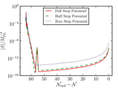
(a) The source term results at all time steps

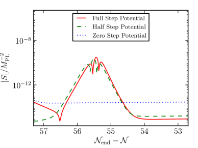
(b) The source term results around the feature

Figure 7: The source term results for the full (red solid line), half (green dashed line) and zero (blue dotted line) step potentials for scale $k_{\mathrm{WMAP}}$.

(a) The source term results at all time steps

(b) The source term results around the feature

Figure 8: The source term results for the full (red solid line), half (green dashed line) and zero (blue dotted line) bump potentials for scale $k_{\mathrm{WMAP}}$.

At second order the differences in the models make themselves even more apparent. Figure 9 shows the second order solution for $k_{\mathrm{WMAP}}$ again for the full, half and zero step potentials. The amplitude of the step has a marked effect on the amplitude of the second order modes. The differences in the source term before the feature are carried over to the second order result. The magnitude of the second order result is much lower for the full step potential than the the quadratic result. When the amplitude of the step is halved the change in the magnitude is also reduced. The difference between the full and quadratic results is at least an order of magnitude and the detailed cause of this difference is a subject for further investigation. The results for the bump potential are shown in Figure 10. Here the effect of the feature is only evident around the bump, again carrying over the result from the source term values.

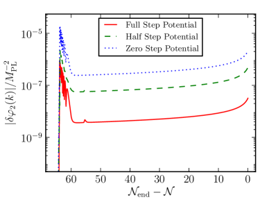
(a) The second order results at all time steps

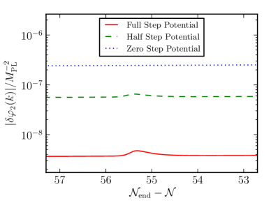
(b) The second order results around the feature

Figure 9: The second order results for the full (red solid line), half (green dashed line) and zero (blue dotted line) step potentials for scale $k_{\mathrm{WMAP}}$.

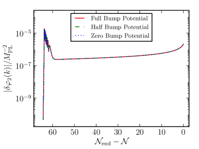
(a) The second order results at all time steps

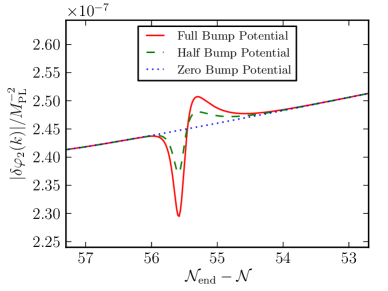
(b) The second order results around the feature

Figure 10: The second order results for the full (red solid line), half (green dashed line) and zero (blue dotted line) bump potentials for scale $k_{\mathrm{WMAP}}$.

4.3 Sub- and Super-Horizon Features

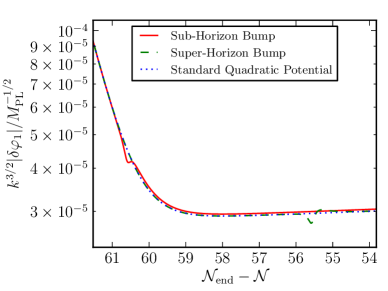
(a) The first order results around the feature.

(b) The source term results around the feature.

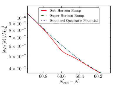
(c) The second order results around the feature.

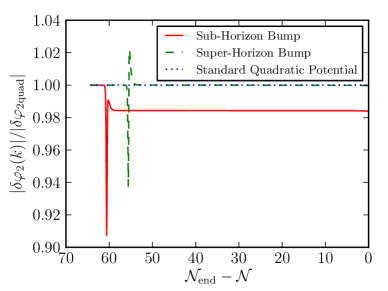
(d) The ratio of the second order results for the sub- and super-horizon bump compared to the standard quadratic result.

Figure 11: The first order and source term results for the bump potential when the bump is inside the horizon when $\varphi_{\rm{b}}=15.5M_{\mathrm{PL}}$ (red solid line) or outside the horizon when $\varphi_{\rm{b}}=14.8M_{\mathrm{PL}}$ (green dashed line). The standard quadratic potential results are also shown as the blue dotted line and all the results are for the scale $k_{\mathrm{WMAP}}$.

For different $k$ modes the feature occurs when the mode is either inside or outside the horizon. When the mode has already crossed the horizon the result is as in Figure 5. Modes which are inside the horizon when they encounter the feature in the potential are not affected in the same way. Of course the location of the bump can also be changed by varying the $\varphi_{\rm{b}}$ parameter in the potential. In Figure 11 the first order power spectrum and source term results are plotted for a potential where the bump feature is located inside the horizon and $\varphi_{\rm{b}}=15.5M_{\mathrm{PL}}$ and compared with the standard quadratic potential and the normal bump potential where $\varphi_{\rm{b}}=14.8M_{\mathrm{PL}}$. When the bump is sub-horizon (the red solid line in Figure 11) the first order results are slightly perturbed from the standard result, reaching a slightly altered magnitude after horizon crossing. This does not happen for the super-horizon bump (green dashed line) which asymptotes back to the quadratic result after the feature.

The source term results also differ depending on the location of the bump. When the bump is sub-horizon the change in the magnitude of the source term is much more suppressed compared to when the bump is outside the horizon. In the second case the oscillations of nearly all the modes have already been dampened by the time the feature is encountered. The convolution integral over the modes is then much more affected by the change in the first order perturbations around the feature. In contrast when the bump is sub-horizon, at least for the $k_{\mathrm{WMAP}}$ scale, most of the other scales considered in the integral are still oscillating and the net effect is a small change in the magnitude of the source term. At second order the results are similar to first order. The sub-horizon bump slightly changes the magnitude away from the quadratic result, in this case reducing it. This change is kept beyond the horizon in contrast to the super-horizon case where the result asymptotes smoothly back to the quadratic one beyond the feature. Figure 11d shows the ratio of the sub- and super-horizon bump second order results to the standard quadratic result. Following the sub-horizon bump the difference between the results is of the order of 2% whereas for the super-horizon bump the results are indistinguishable from the quadratic results after the feature region.  

In this section we have outlined the main results of our new numerical calculation. We have shown that the source term results using the full non-slow-roll equation (2.2) are more damped than the corresponding slow-roll results. We have demonstrated the new code by using feature potentials with a step and a bump added to the standard quadratic potential. Depending on the position of the feature and the form of the addition to the potential the effects of the feature can be seen in the source term and second order results beyond the feature itself. Whether the feature is sub- or super-horizon for a particular mode also affects the subsequent evolution.

5 Discussion and Conclusion

We describe in this paper the numerical solution of the full Klein-Gordon equation for a single scalar field at second order in cosmological perturbation theory. We use gauge-invariant variables in the flat gauge without imposing the slow-roll approximation or using the large scale limit. This is an extension of previous work, that relied on the slow-roll approximation to calculate the source term [8]. We have made this extended code publicly available (it can be downloaded from the website [24]). To validate and test the code, we studied several single field potentials, including step and bump extensions of the simple chaotic inflation potential, which violate one of the slow-roll conditions.

We have shown that feature potentials affect the source and second order results and at least for the step potential these effects are apparent throughout the evolution of the modes and not just in a narrow region around the feature. This is consistent with the higher order derivatives of the potentials being non-zero, or at least having different values when computed without a feature. Is this a problem for feature potentials? At one level the feature potentials we have used are theoretical toy models which are not motivated by high energy physics. At first order in perturbation theory the $\tanh$ and $\cosh$ additions to the quadratic potential work to localise the deviation to a specific region. This is clearly not the case at second order for the step potential. To replicate this behaviour at second order, a restricted version of the step or bump potentials could be used. However, one main benefit of using $\tanh$ or $\cosh$ is that they smoothly asymptote to the original potential away from the feature. Any attempted patching together of featureless potential and feature in a specific region would have to be carefully constructed to avoid discontinuities in the derivatives of the potential. In contrast the results for the bump potential are only affected in a narrow region around the feature. It is interesting to note, that a step-potential of the form (4.1) has recently been used to study the generation of magnetic fields in the early universe [33].

Somewhat surprising was the effect the small sub-horizon bump had on the evolution of the second order field fluctuation $\delta\varphi_{2}$ on large scales, see Figure 11. Sub-horizon effects like this can only be studied by codes like the one described here, but would not be calculable by super-horizon codes, such as the recently proposed one in Refs. [34, 35]. However, it is not clear yet whether this change in $\delta\varphi_{2}$ would translate into observational consequences, such as a change in $f_{\mathrm{NL}}$. We are cautiously optimistic that it might have an observable effect, but postpone a detailed calculation to future work. In this future work we plan to study more complicated and also more interesting potentials than in Section 4, and also hope to extend the code to allow the evolution of more than one field. In addition, to our knowledge there is currently no expression that exists in closed form for $\zeta_{2}$ or $\mathcal{R}_{2}$ which is valid on all scales without imposing slow-roll. Constructing such an expression should be possible and would allow for direct calculation of the evolution of $\zeta_{2}$ and we look forward to making progress on this issue. A recent work discussing the numerical calculation of $f_{\mathrm{NL}}$ used lattice field theory simulations [36]. Whether in future this method will prove more efficient than the one discussed here will depend on detailed comparative analyses which are beyond the scope of the present article. Other recent work by Takamizu et al. [37] matched a perturbative solution for the curvature of a single field model inside the horizon to a non-linear solution outside the horizon which uses a gradient expansion. The authors claim this goes beyond the limitations of the $\delta N$ formalism and can also deal with temporary violations of slow-roll. It would be interesting in future work to compare the results of our approach with those of Takamizu et al. especially in the region where the matching of the solutions takes place. Gong, Noh and Hwang have also looked at higher order perturbations [38]. Their work concentrates on evolving the convolution kernels of the curvature perturbation but only for large scales with slow roll parameters equated to zero. The “Generalized Slow Roll” approximation can also be used to investigate models which break slow roll transiently around a feature [10, 39, 40]. Adshead et al. [40] have demonstrated calculations of the bispectrum of a single field model and observe good agreement with analytic results. However, this approach is limited to superhorizon scales only and can only be applied when there is a single degree of freedom. Another natural application and extension of our code is to apply it to other problems that have evolution equations of a similar form. As pointed out in the introduction, two immediate applications might be the numerical study of the generation of gravitational waves at second order [22] (see Ref. [41] for earlier numerical work) and the generation of vorticity [23]. In both cases the source term of the second order quantities is given by a convolution integral quadratic in first order quantities.

Finally, the numerical calculation of the convolution integral requires cutoffs to be implemented at both large and small scales. We have explained the cutoffs we use explicitly in Refs. [8, 29] and refer the interested reader to the discussions contained therein. It will be interesting to implement in future work different cut-off schemes, as outlined for example in Refs. [42, 43]. Our current choice of cut-offs is pragmatic, however there may be physical considerations for adopting a different cut-off scheme, which would impact on the higher order perturbations and therefore affect the non-linear observables.

Appendix A Appendix

The methods adopted for the study of first order perturbations can be extended at second order to find gauge invariant quantities. Recall that scalar quantities such as the inflaton field, $\varphi$, can be split into an homogeneous background, $\varphi_{0}$, and inhomogeneous perturbations. Up to second order $\varphi$ becomes

$$\varphi(\eta,x^{\mu})=\varphi_{0}(\eta)+\delta\varphi_{1}(\eta,x^{i})+\frac{1}{2}\delta\varphi_{2}(\eta,x^{i})\,.$$ (A.1)

The metric tensor $g_{\mu\nu}$ must also be perturbed up to second order. Here we consider only the scalar metric perturbations [26]:

$$g_{00} =-a^{2}\left(1+2\phi_{1}+\phi_{2}\right)\,,$$

$$g_{0i} =a^{2}\left(B_{1}+\frac{1}{2}B_{2}\right)_{,i}\,,$$

$$g_{ij} =a^{2}\left[\left(1-2\psi_{1}-\psi_{2}\right)\delta_{ij}+2E_{1,ij}+E_{2,ij}\right]\,,$$ (A.2)

where $\delta_{ij}$ is the flat background metric, $\phi_{1}$ and $\phi_{2}$ are the lapse functions at first and second order, $\psi_{1}$ and $\psi_{2}$ are the curvature perturbations, and $B_{1}$, $B_{2}$, $E_{1}$ and $E_{2}$ are the scalar perturbations describing the shear. As well as the first order transformation vector, there is a second order transformation vector and they are both given by

$$\xi_{1}^{\mu}=(\alpha_{1},\beta_{1,}^{~{}~{}i})\,,\quad\xi_{2}^{\mu}=(\alpha_{2},\beta_{2,}^{~{}~{}i})\,,$$ (A.3)

where the spatial vector part of the transformation has been ignored.

The transformation of a second order scalar quantity (such as $\delta\varphi_{2}$) is given by [44, 26]:

$$\widetilde{\delta\varphi_{2}}=\delta\varphi_{2}+\varphi_{0}^{\prime}\alpha_{2}+\alpha_{1}\left(\varphi_{0}^{\prime\prime}\alpha_{1}+\varphi_{0}^{\prime}\alpha_{1}^{\prime}+2\delta\varphi_{1}^{\prime}\right)+\left(2\delta\varphi_{1}+\varphi_{0}^{\prime}\alpha_{1}\right)_{,i}\beta_{1,}^{~{}~{}i}\,,$$ (A.4)

where a tilde ($\widetilde{~{}}$) denotes a transformed quantity. The metric curvature perturbation transformation at first order is straightforward, $\widetilde{\psi_{1}}=\psi_{1}-\mathcal{H}\alpha_{1}$, but at second order it becomes more complicated [25, 26]:

$$\widetilde{\psi_{2}}=\psi_{2}-\mathcal{H}\alpha_{2}-\frac{1}{4}\mathcal{X}^{k}_{~{}k}+\frac{1}{4}\nabla^{-2}\mathcal{X}^{ij}_{~{}~{}ij}\,,$$ (A.5)

where $\mathcal{X}_{ij}$ is given by

$$\mathcal{X}_{ij}\equiv 2\Big{[}\left(\mathcal{H}^{2}+\frac{a^{\prime\prime}}{a}\right)\alpha_{1}^{2}+\mathcal{H}\left(\alpha_{1}\alpha_{1}^{\prime}+\alpha_{1,k}\xi_{1}^{~{}k}\right)\Big{]}\delta_{ij}$$

$$+4\Big{[}\alpha_{1}\left(C_{1ij}^{\prime}+2\mathcal{H}C_{1ij}\right)+C_{1ij,k}\xi_{1}^{~{}k}+C_{1ik}\xi_{1~{}~{},j}^{~{}k}+C_{1kj}\xi_{1~{}~{},i}^{~{}k}\Big{]}$$

$$+2\left(B_{1i}\alpha_{1,j}+B_{1j}\alpha_{1,i}\right)+4\mathcal{H}\alpha_{1}\left(\xi_{1i,j}+\xi_{1j,i}\right)-2\alpha_{1,i}\alpha_{1,j}+2\xi_{1k,i}\xi_{1~{}~{},j}^{~{}k}$$

$$+\alpha_{1}\left(\xi_{1i,j}^{\prime}+\xi_{1j,i}^{\prime}\right)+\left(\xi_{1i,jk}+\xi_{1j,ik}\right)\xi_{1}^{~{}k}+\xi_{1i,k}\xi_{1~{}~{},j}^{~{}k}+\xi_{1j,k}\xi_{1~{}~{},i}^{~{}k}$$

$$+\xi_{1i}^{\prime}\alpha_{1,j}+\xi_{1j}^{\prime}\alpha_{1,i}\,,$$ (A.6)

and $B_{1i}$ and $C_{1ij}$ are defined as

$$B_{1i}=B_{1,i}\,,\quad C_{1ij}=-\psi_{1}\delta_{ij}+E_{1,ij}\,.$$ (A.7)

Working in the uniform curvature gauge, where spatial 3-hypersurfaces are flat, implies that

$$\widetilde{\psi}_{1}=\widetilde{\psi}_{2}=\widetilde{E}_{1}=\widetilde{E}_{2}=0\,.$$ (A.8)

These relations can be used at first and then at second order to define gauge invariant variables. The first order transformation variables in the flat gauge satisfy $\alpha_{1}=\psi_{1}/\mathcal{H}$ and $\beta_{1}=-E_{1}$. At second order, for the transformation of scalar quantities, as in Eq. (A.4), we require only $\alpha_{2}$. This is found by using Eq. (A.5) to have the form

$$\alpha_{2}=\frac{\psi_{2}}{\mathcal{H}}+\frac{1}{4\mathcal{H}}\left[\nabla^{-2}\mathcal{X}^{ij}_{~{}~{},ij}-\mathcal{X}^{k}_{k}\right]\,,$$ (A.9)

where the first order gauge variables have been substituted into $\mathcal{X}_{ij}$.

The Sasaki-Mukhanov variable, i.e., the field perturbation on uniform curvature hypersurfaces [45, 46], is given at first order by

$$\widetilde{\delta\varphi_{1}}=\delta\varphi_{1}+\frac{\varphi_{0}^{\prime}}{\mathcal{H}}\psi_{1}\,.$$ (A.10)

At second order the Sasaki-Mukhanov variable becomes more complicated [5, 44]:

$$\widetilde{\delta\varphi_{2}}= \delta\varphi_{2}+\frac{\varphi_{0}^{\prime}}{\mathcal{H}}\psi_{2}+\frac{\varphi_{0}^{\prime}}{4\mathcal{H}}\left(\nabla^{-2}\mathcal{X}^{ij}_{~{}~{},ij}-\mathcal{X}^{k}_{k}\right)$$

$$+\frac{\psi_{1}}{\mathcal{H}^{2}}\Big{[}\varphi_{0}^{\prime\prime}{\psi_{1}}+\varphi_{0}^{\prime}\left(\psi_{1}^{\prime}-\frac{\mathcal{H}^{\prime}}{\mathcal{H}}\psi_{1}\right)+2\mathcal{H}\delta\varphi_{1}^{\prime}\Big{]}+\left(2\delta\varphi_{1}+\frac{\varphi_{0}^{\prime}}{\mathcal{H}}\psi_{1}\right)_{,k}\xi_{1\mathrm{flat}}^{k}\,,$$ (A.11)

where $\xi_{1\mathrm{flat}}=-E_{1,i}$. From now on we will drop the tildes and only refer to variables calculated in the flat gauge. The potential of the scalar field can also be separated into homogeneous and perturbed sectors:

$$V(\varphi) =V_{0}+\delta V_{1}+\frac{1}{2}\delta V_{2}\,,\quad$$ (A.12)

$$\delta V_{1} =V_{,\varphi}\delta\varphi_{1}\,,\quad$$ (A.13)

$$\delta V_{2} =V_{,\varphi\varphi}\delta\varphi_{1}^{2}+V_{,\varphi}\delta\varphi_{2}\,.$$ (A.14)

The Klein-Gordon equations are found by requiring the perturbed energy-momentum tensor $T_{\mu\nu}$ to obey the energy conservation equation $\nabla_{\mu}T^{\mu\nu}=0$ (see for example Ref. [5]). For the background field, $\varphi_{0}$, the Klein-Gordon equation is

$$\varphi_{0}^{\prime\prime}+2\mathcal{H}\varphi_{0}^{\prime}+a^{2}V_{,\varphi}=0\,.$$ (A.15)

The first order equation is

$$\delta\varphi_{1}^{\prime\prime}+2\mathcal{H}\delta\varphi_{1}^{\prime}+2a^{2}V_{,\varphi}\phi_{1}-\nabla^{2}\delta\varphi_{1}-\varphi_{0}^{\prime}\nabla^{2}B_{1}-\varphi_{0}^{\prime}\phi^{\prime}_{1}+a^{2}V_{,\varphi\varphi}\delta\varphi_{1}=0\,,$$ (A.16)

and the second order one is given by

$$\delta\varphi_{2}^{\prime\prime} +2\mathcal{H}\delta\varphi_{2}^{\prime}-\nabla^{2}\delta\varphi_{2}+a^{2}V_{,\varphi\varphi}\delta\varphi_{2}+a^{2}V_{,\varphi\varphi\varphi}(\delta\varphi_{1})^{2}+2a^{2}V_{,\varphi}\phi_{2}-\varphi_{0}^{\prime}\left(\nabla^{2}B_{2}+\phi_{2}^{\prime}\right)$$

$$+4\varphi_{0}^{\prime}B_{1,k}\phi_{1,}^{~{}k}+2\left(2\mathcal{H}\varphi_{0}^{\prime}+a^{2}V_{,\varphi}\right)B_{1,k}B_{1,}^{~{}k}+4\phi_{1}\left(a^{2}V_{,\varphi\varphi}\delta\varphi_{1}-\nabla^{2}\delta\varphi_{1}\right)$$

$$+4\varphi_{0}^{\prime}\phi_{1}\phi_{1}^{\prime}-2\delta\varphi_{1}^{\prime}\left(\nabla^{2}B_{1}+\phi_{1}^{\prime}\right)-4{\delta\varphi_{1}^{\prime}}_{,k}B_{1,}^{~{}k}$$

$$=0\,,$$ (A.17)

where all the variables are now in the flat gauge.

In order to write the Klein-Gordon equations in closed form, the Einstein field equations are also required at first and second order. These are not reproduced here, but are presented for example in Section II B of Ref. [7].

References

- [1] NASA/WMAP Team, “WMAP mission website.” http://wmap.gsfc.nasa.gov.
- [2] ESA/Planck Team, “Planck mission website.” http://www.esa.int/planck.
- [3] A. R. Liddle and D. H. Lyth, Cosmological Inflation and Large-Scale Structure. Cambridge University Press, April, 2000.
- [4] S. M. Leach, M. Sasaki, D. Wands, and A. R. Liddle, “Enhancement of superhorizon scale inflationary curvature perturbations,” Phys. Rev. D64 (2001) 023512, arXiv:astro-ph/0101406.
- [5] K. A. Malik, “Gauge-invariant perturbations at second order: Multiple scalar fields on large scales,” JCAP 0511 (2005) 005, arXiv:astro-ph/0506532.
- [6] K. A. Malik, D. Seery, and K. N. Ananda, “Different approaches to the second order Klein-Gordon equation,” Class. Quant. Grav. 25 (2008) 175008, arXiv:0712.1787 [astro-ph].
- [7] K. A. Malik, “A not so short note on the Klein-Gordon equation at second order,” JCAP 0703 (2007) 004, arXiv:astro-ph/0610864.
- [8] I. Huston and K. A. Malik, “Numerical calculation of second order perturbations,” JCAP 0909 (2009) 019, arXiv:0907.2917 [astro-ph.CO].
- [9] J. A. Adams, B. Cresswell, and R. Easther, “Inflationary perturbations from a potential with a step,” Phys. Rev. D64 (2001) 123514, arXiv:astro-ph/0102236.
- [10] E. D. Stewart, “The spectrum of density perturbations produced during inflation to leading order in a general slow-roll approximation,” Phys. Rev. D65 (2002) 103508, arXiv:astro-ph/0110322.
- [11] J. Choe, J.-O. Gong, and E. D. Stewart, “Second order general slow-roll power spectrum,” JCAP 0407 (2004) 012, arXiv:hep-ph/0405155.
- [12] M. Joy, A. Shafieloo, V. Sahni, and A. A. Starobinsky, “Is a step in the primordial spectral index favored by CMB data ?,” JCAP 0906 (2009) 028, arXiv:0807.3334 [astro-ph].
- [13] J. Hamann, A. Shafieloo, and T. Souradeep, “Features in the primordial power spectrum? A frequentist analysis,” JCAP 1004 (2010) 010, arXiv:0912.2728 [astro-ph.CO].
- [14] D. K. Hazra, M. Aich, R. K. Jain, L. Sriramkumar, and T. Souradeep, “Primordial features due to a step in the inflaton potential,” JCAP 1010 (2010) 008, arXiv:1005.2175 [astro-ph.CO].
- [15] X. Chen, R. Easther, and E. A. Lim, “Generation and Characterization of Large Non-Gaussianities in Single Field Inflation,” JCAP 0804 (2008) 010, arXiv:0801.3295 [astro-ph].
- [16] X. Chen, R. Easther, and E. A. Lim, “Large non-Gaussianities in single field inflation,” JCAP 0706 (2007) 023, arXiv:astro-ph/0611645.
- [17] A. A. Starobinsky, “Dynamics of Phase Transition in the New Inflationary Universe Scenario and Generation of Perturbations,” Phys. Lett. B117 (1982) 175–178.
- [18] A. A. Starobinsky, “Multicomponent de Sitter (Inflationary) Stages and the Generation of Perturbations,” JETP Lett. 42 (1985) 152–155.
- [19] D. S. Salopek and J. R. Bond, “Nonlinear evolution of long wavelength metric fluctuations in inflationary models,” Phys. Rev. D42 (1990) 3936–3962.
- [20] M. Sasaki and E. D. Stewart, “A General analytic formula for the spectral index of the density perturbations produced during inflation,” Prog. Theor. Phys. 95 (1996) 71–78, arXiv:astro-ph/9507001.
- [21] D. H. Lyth, K. A. Malik, and M. Sasaki, “A general proof of the conservation of the curvature perturbation,” JCAP 0505 (2005) 004, arXiv:astro-ph/0411220.
- [22] K. N. Ananda, C. Clarkson, and D. Wands, “The cosmological gravitational wave background from primordial density perturbations,” Phys. Rev. D75 (2007) 123518, arXiv:gr-qc/0612013.
- [23] A. J. Christopherson, K. A. Malik, and D. R. Matravers, “Vorticity generation at second order,” Phys. Rev. D79 (2009) 123523, arXiv:0904.0940 [astro-ph.CO].
- [24] I. Huston, “Pyflation: Cosmological perturbations for Python.” http://pyflation.ianhuston.net, 2011–.
- [25] K. A. Malik and D. R. Matravers, “A Concise Introduction to Perturbation Theory in Cosmology,” Class. Quant. Grav. 25 (2008) 193001, arXiv:0804.3276 [astro-ph].
- [26] K. A. Malik and D. Wands, “Cosmological perturbations,” Phys. Rept. 475 (2009) 1–51, arXiv:0809.4944 [astro-ph].
- [27] H. Noh and J.-c. Hwang, “Second-order perturbations of the Friedmann world model,” Phys. Rev. D69 (2004) 104011.
- [28] A. Vretblad, Fourier Analysis and Its Applications (Graduate Texts in Mathematics). Springer, 2005.
- [29] I. Huston, “Constraining Inflationary Scenarios with Braneworld Models and Second Order Cosmological Perturbations,” arXiv:1006.5321 [astro-ph.CO].
- [30] D. S. Salopek, J. R. Bond, and J. M. Bardeen, “Designing Density Fluctuation Spectra in Inflation,” Phys. Rev. D40 (1989) 1753.
- [31] C. Ringeval, “The exact numerical treatment of inflationary models,” Lect. Notes Phys. 738 (2008) 243–273, arXiv:astro-ph/0703486.
- [32] J. Martin and C. Ringeval, “Inflation after WMAP3: Confronting the slow-roll and exact power spectra to CMB data,” JCAP 0608 (2006) 009, arXiv:astro-ph/0605367.
- [33] R. Durrer, L. Hollenstein, and R. K. Jain, “Can slow roll inflation induce relevant helical magnetic fields?,” arXiv:1005.5322 [astro-ph.CO].
- [34] D. J. Mulryne, D. Seery, and D. Wesley, “Moment transport equations for non-Gaussianity,” JCAP 1001 (2010) 024, arXiv:0909.2256 [astro-ph.CO].
- [35] D. J. Mulryne, D. Seery, and D. Wesley, “Moment transport equations for the primordial curvature perturbation,” arXiv:1008.3159 [astro-ph.CO].
- [36] N. Barnaby, “On Features and Nongaussianity from Inflationary Particle Production,” Phys.Rev. D82 (2010) 106009, arXiv:1006.4615 [astro-ph.CO].
- [37] Y.-i. Takamizu, S. Mukohyama, M. Sasaki, and Y. Tanaka, “Non-Gaussianity of superhorizon curvature perturbations beyond N formalism,” JCAP 1006 (2010) 019, arXiv:1004.1870 [astro-ph.CO].
- [38] J.-O. Gong, H. Noh, and J.-c. Hwang, “Non-linear corrections to inflationary power spectrum,” JCAP 1104 (2011) 004, arXiv:1011.2572 [astro-ph.CO].
- [39] C. Dvorkin and W. Hu, “Generalized Slow Roll for Large Power Spectrum Features,” Phys. Rev. D81 (2010) 023518, arXiv:0910.2237 [astro-ph.CO].
- [40] P. Adshead, W. Hu, C. Dvorkin, and H. V. Peiris, “Fast Computation of Bispectrum Features with Generalized Slow Roll,” arXiv:1102.3435 [astro-ph.CO].
- [41] D. Baumann, P. J. Steinhardt, K. Takahashi, and K. Ichiki, “Gravitational Wave Spectrum Induced by Primordial Scalar Perturbations,” Phys.Rev. D76 (2007) 084019, arXiv:hep-th/0703290 [hep-th].
- [42] G. Marozzi, M. Rinaldi, and R. Durrer, “On infrared and ultraviolet divergences of cosmological perturbations,” arXiv:1102.2206 [astro-ph.CO].
- [43] D. Seery, “Infrared effects in inflationary correlation functions,” Class.Quant.Grav. 27 (2010) 124005, arXiv:1005.1649 [astro-ph.CO].
- [44] K. A. Malik and D. Wands, “Evolution of second order cosmological perturbations,” Class. Quant. Grav. 21 (2004) L65–L72, arXiv:astro-ph/0307055.
- [45] M. Sasaki, “Large Scale Quantum Fluctuations in the Inflationary Universe,” Prog. Theor. Phys. 76 (1986) 1036.
- [46] V. F. Mukhanov, “Quantum Theory of Gauge Invariant Cosmological Perturbations,” Sov. Phys. JETP 67 (1988) 1297–1302.