Bistable non-volatile elastic membrane memcapacitor exhibiting chaotic behavior

Abstract

We suggest a realization of a bistable non-volatile memory capacitor (memcapacitor). Its design utilizes a strained elastic membrane as a plate of a parallel-plate capacitor. The applied stress generates low and high capacitance configurations of the system. We demonstrate that a voltage pulse of an appropriate amplitude can be used to reliably switch the memcapacitor into the desired capacitance state. Moreover, charged-voltage and capacitance-voltage curves of such a system demonstrate hysteresis and transition into a chaotic regime in a certain range of ac voltage amplitudes and frequencies. Membrane memcapacitor connected to a voltage source comprises a single element nonautonomous chaotic circuit.

I Introduction

Currently, there is a strong interest in resistive, capacitive and inductive elements with memory Di Ventra et al. (2009). The memory feature extends functionality of such elements and leads to novel circuit applications Pershin et al. (2009); Snider (2008). The main recent progress in this area is in the field of memory resistive (memristive) systems Chua (1971); Chua and Kang (1976); Strukov et al. (2008) that can be potentially used in both digital Strukov and Williams (2009) and analog Pershin et al. (2009); Jo et al. (2010); Pershin and Di Ventra (2010a); Snider (2008); Pershin and Di Ventra (2010b) applications.

This article concerns less studied memcapacitive systems. By definition Di Ventra et al. (2009), a voltage-controlled memcapacitive system is given by the equations

$$q(t) = C\left(x,V_{C},t\right)V_{C}(t)$$ (1)

$$\dot{x} = f\left(x,V_{C},t\right)$$ (2)

where $q(t)$ is the charge on the capacitor at time $t$, $V_{C}(t)$ is the applied voltage, $C$ is the memcapacitance, $x$ is a set of $n$ state variables describing the internal state of the system, and $f$ is a continuous $n$-dimensional vector function. It is important that the memcapacitance $C$ depends on the state of the system and can vary in time. Several systems showing memcapacitive behavior has been identified including vanadium dioxide metamaterials Driscoll et al. (2009), ionic systems Lai et al. (2009); Krems et al. (2010) and superlattice memcapacitors Martinez-Rincon et al. (2010).

In this paper we suggest a different memcapacitor realization. Our main idea is to replace a plate of a parallel-plate capacitor by a strained elastic membrane as we demonstrate schematically in Fig. 1. The applied stress bends the membrane up or down, allowing for two equilibrium positions. When the membrane is in the position closer to the bottom plate, the capacitance of the device is higher (for simplicity, this configuration is called ”1”). When the membrane is bent up, the system has a lower capacitance denoted by ”0”. Both states are perfectly stables, providing a better non-volatile information storage capability than the known designs of memcapacitors Driscoll et al. (2009); Lai et al. (2009); Krems et al. (2010); Martinez-Rincon et al. (2010); Pershin and Di Ventra (2011). We show below that the information can be written into the memcapacitor state by applying a single voltage pulse. An interesting feature of such a device is a chaotic behavior regime achievable within a certain range of parameters.

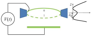
Figure 1: Schematic of a bistable non-volatile elastic membrane memcapacitor connected to a voltage source $V(t)$. The top plate of a regular parallel-plate capacitor is replaced by a flexible strained membrane. Because of two equilibrium positions of the membrane (represented by a double-well potential sketched on the right hand side of the figure), stable high and low capacitance configurations are possible in such a system.

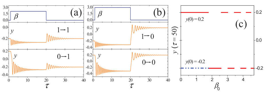
Figure 2: Dynamics of membrane memcapacitor subjected to a single voltage pulse. It is shown in (a) ((b)) that a $\beta_{0}=2.1$ ($\beta_{0}=2.8$) pulse drives the system into the final high (low) capacitance state independently of the initial state of the membrane. The final state (at the indicated time) is shown as a function of the pulse amplitude $\beta_{0}=\left[2\pi/\left(\omega_{0}\,d\right)\right]\sqrt{C_{0}/\left(2\,m\right)}\,V_{0}$ in (c). The red (blue double-dot-dash) curve represents the final position of the membrane when the initial state is ”0” (”1”). Below $\beta_{0}=1.77$ the final state depends on the initial one. Above $\beta_{0}=1.77$ both curves overlap and the final state is independent on the initial state of membrane. The parameters used in these simulations are $y_{0}=0.2$ and $\Gamma=0.7$.

II Model

Let us consider an air gap capacitor composed by a fixed plate and a flexible strained membrane (bottom and top plates in Fig. 1). For the sake of simplicity, we describe the membrane by a single variable $z$ (the effective displacement of the membrane from its middle (non strained) position) and calculate the capacitance using a parallel plates capacitor model. The effect of the stress can be described by a double well potential of the form $U(z)\propto\left(z^{2}-z_{0}^{2}\right)^{2}$, where $\pm z_{0}$ are the equilibrium positions of the membrane. In addition, there is an attractive electrostatic interaction between the charges on the fixed plate and membrane. The electric force acting on the membrane is given by the product of the charge on it, $q$, times the electric field produced by the charge on the fixed plate, $-q/\left(2\,\epsilon_{0}\,S\right)$, where $\epsilon_{0}$ is the electric constant and $S$ is the area of the fixed plate.

Introducing a dimensionless variable $y=z/d$, where $d$ is the separation between the bottom plate and middle position of the membrane, we write the relation between the charge $q(t)$ and voltage $V(t)$ and the membrane’s equation of motion as

$$q(t)=\frac{C_{0}}{1+y(t)}V(t)\equiv C(y(t))V(t),$$ (3)

$$\frac{\textnormal{d}}{\textnormal{d}\tau}\left[\begin{array}[]{c}y\\ \\ \dot{y}\end{array}\right]=\left[\begin{array}[]{c}\dot{y}\\ -4\pi^{2}\,y\,\left(\frac{y^{2}}{y^{2}_{0}}-1\right)-\Gamma\,\dot{y}-\frac{\beta^{2}(\tau)}{(1+y)^{2}}\end{array}\right]$$ (4)

where $C_{0}=\epsilon_{0}\,S/d$, $y_{0}=z_{0}/d$, $\Gamma=2\pi\,\gamma/\omega_{0}$, $\gamma$ is the damping constant, $\omega_{0}$ is the natural angular frequency of the system, $\beta(t)=\left[2\pi/\left(\omega_{0}\,d\right)\right]\sqrt{C_{0}/\left(2\,m\right)}\,V(t)$, $m$ is the mass of the membrane and the time derivatives in Eq. (4) are taken with respect to the dimensionless time $\tau=t\,\omega_{0}/\left(2\pi\right)$. Eqs. (3) and (4) have the general form given by Eqs. (1) and (2) and, therefore, the membrane memcapacitor is a second-order voltage-controlled memcapacitive system.

III Initialization of memcapacitor state and hysteresis loops

A single voltage pulse of an appropriate duration and amplitude can be used for the purpose of the memcapacitor state initialization. Specifically, we demonstrate below that depending on the pulse amplitude, the memcapacitor can be controllably set into the state ”0” or ”1”. The initialization of the memcapacitor state can not rely on the electrostatic interaction alone because this interaction in the capacitor is always attractive. Therefore, in order to obtain the state ”0”, a higher amplitude pulse should be applied such that the restoring elastic force, when the voltage pulse ends, allows overcoming the potential barrier shown in Fig. 1.

Figs. 2(a) and 2(b) show simulation results of the memcapacitor dynamics obtained as a numerical solution of Eq. (4) for two different values of the applied pulse amplitude. When a lower amplitude $\beta_{0}=2.1$ pulse is applied to the system for a long enough time, the membrane first finds an equilibrium position at this value of voltage. This position is independent on the initial state of the membrane in the switching regime ($\beta_{0}>1.77$ in our simulations, see Figs. 2(a) and 2(c) for details). Then, when the voltage drops to zero, the membrane oscillates around $-y_{0}$ and eventually the equilibrium position ”1” is reached.

When a higher amplitude pulse ($\beta_{0}=2.8$) is applied (see Fig. 2(b)), the membrane is attracted down stronger before being released. As a result, when the pulse ends, the membrane goes up and stays in the low capacitance configuration ”0”. With a further increase of the pulse amplitude, the final state of the membrane can be again ”1” and then ”0”, etc. Such periodic situation is clearly seen in Fig. 2(c). Note that in the switching regime ($\beta_{0}>1.77$) the final state of the membrane does not depend on its initial state.

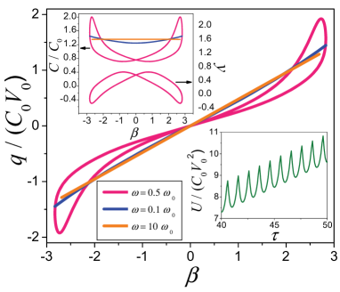
Figure 3: $q-V$ and $C-V$ (top curves in the top inset) curves for a membrane memcapacitor calculated when a sinusoidal voltage is applied. The bottom curve in the top inset represents $y(\beta)$ at $\omega=0.5\omega_{0}$. Parameters used in this simulation are the same as in Fig. 2 and $\beta=\beta_{0}\sin(\omega t)$ with $\beta_{0}=2.8$. The graphs demonstrate a periodic steady-state regime beyond an initial equilibration interval $(\tau\gtrsim 30)$. Limits to linear (orange) and non-linear (blue) behaviors are obtained at high and low frequencies. Hysteresis loops are seen at intermediate frequencies. The bottom inset is the energy dissipated by the system, given by $U=\int{V\,dq}$, calculated at $\omega=0.5\omega_{0}$.

When the membrane memcapacitor is subjected to ac voltage, its dynamics can be periodic or chaotic depending on the frequency and amplitude of the ac voltage. In this section we consider only the periodic case. The chaotic behavior is discussed in Sec. IV. A numerical solution of Eqs. (3,4) with $\beta(t)=\beta_{0}\sin(\omega t)$ is plotted in Fig. 3 for three different values of the applied voltage frequency. The hysteresis curves demonstrate typical behavior of memory elements Di Ventra et al. (2009): non-linear dependencies at lower frequencies, pinched hysteresis loops at intermediate frequencies and linear behavior at higher frequencies.

The hysteresis observed in Fig. 3 at $\omega=0.5\omega_{0}$ is basically related to the well-known phase shift between periodic applied force and position of a driven mechanical system. Basically, this effect originates from the membrane’s inertia as well as from the fact that a finite time is required to dissipate instantaneous energy stored, e.g., in the elastic degree of freedom of the membrane. Since the electrostatic interaction between capacitor’s plates is always attractive, the $C-V$ curve is symmetric with respect to $\beta=0$ and the membrane experiences a driving force of the doubled frequency of ac voltage. The pinched behavior additionally proofs that the system is a memory capacitive device. The bottom inset in Fig. 3 shows the energy dissipated by the device for 10 cycles in the steady regime. Because of the damping term in Eq. (4), the membrane memcapacitor is a dissipative system.

IV Chaotic Behavior

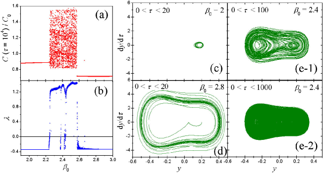
Figure 4: Chaotic behavior of the membrane memcapacitor subjected to ac-voltage ($\beta=\beta_{0}\sin(\omega t)$). The value of capacitance (a) at $\tau=10^{4}$ and the Largest Lyapunov exponent (b) are plotted as a function of the amplitude $\beta_{0}$. The remaining plots (c)-(e) demonstrate trajectories in the phase space ($\dot{y}$ vs. $y$) of the system at three different values of the amplitude $\beta_{0}$. Plots (c) and (d) show a periodic steady-state behavior, and (e) represents the ergodic behavior at $\beta_{0}=2.4$. Calculation parameters are the same as in Fig. 2 and $\omega=0.5\,\omega_{0}$.

Most experts would agree defining chaos as the aperiodic, long-term behavior of a bounded, deterministic system that exhibits sensitive dependence on initial conditions and system parameters Sprott (2003). In this section, we demonstrate that the membrane memcapacitor described by equation (4) can exhibit chaotic behavior. In particular, chaotic regime is observed in numerical simulations for a specific range of amplitudes and frequencies of the applied sinusoidal voltage $V=V_{0}\sin(\omega t)$.

Specifically, in order to explore chaotic properties of the system, let us investigate how the state of the memcapacitor (at a long selected moment of time) depends on one parameter of the system, such as the ac-voltage amplitude $V_{0}$. For this purpose, we ran multiple simulation of the system dynamics at different values of $\beta_{0}$ and monitor the value of capacitance $C$ at a certain moment of time. Fig. 4(a) shows the value of capacitance evaluated at $\tau=10^{4}$ as a function of the amplitude $\beta_{0}$. This plot demonstrates that at small ($\beta_{0}<2.25$) and high ($\beta_{0}>2.58$) voltages, the system reaches practically the same value of capacitance (at a given time) if the voltage amplitude is slightly changed. However, at intermediate voltages ($2.25<\beta_{0}<2.58$) predictability in the value of the capacitance is lost, which is an indicator of chaotic behavior.

The Largest Lyapunov Exponent (LLE) $\lambda$ is a quantitative measure of chaos Sprott (2003). It is defined for a long time behavior of a single trajectory and is sensitive to the initial conditions of the system. If LLE is positive ($\lambda>0$) the trajectory is chaotic and $\lambda$ is a measure of the average rate at which predictability is lost. On the other hand, if $\lambda\leq 0$ the evolution is not chaotic. We use a standard approach to calculate the LLE Benettin et al. (1980a, b). Fig. 4(b) shows the result of our calculation of LLE as a function of the applied voltage amplitude $\beta_{0}$. The chaotic behavior (positive values of $\lambda$) is clearly observed in the interval $2.25<\beta_{0}<2.58$.

The system trajectories in the phase space ($\dot{y}$ vs. $y$) at low, high and intermediate voltage amplitudes are shown in Fig. 4(c)-(e) correspondingly. If the voltage amplitude is such that $\beta$ is below approximately $2.25$ (Fig. 4(c)), the membrane moves periodically either in the low or high capacitance region. If the voltage amplitude is high ($\beta$ is above $2.58$), a different kind of periodic steady-state solution is observed (see Fig. 4(d)). In this case, the voltage is high enough for the membrane to pass through the barrier between the potential wells generating oscillations of the membrane between the high and low capacitance regions. At both low and high voltage amplitudes, the system dynamics is not chaotic. Finally, at intermediate voltage amplitudes ($2.25<\beta_{0}<2.58$), the system does not reach any steady solution. Figs. 4(e-1) and 4(e-2) show the system trajectories up to two different simulation times ($\tau=100$ and $\tau=1000$). It is evident that the system is ergodic, what is another important manifestation of chaos. In fact, it is not quite surprising that Eq. (4) produces chaotic trajectories. Generally, Eq. (4) can be seen as a modification of the Duffing oscillator equation, whose chaotic properties are well-known Sprott (2003).

V Conclusions

The membrane memcapacitor is a modification of a parallel-plate capacitor, in which one of the plates is replaced by a strained membrane having two equilibrium positions. This feature defines two states (”0” and ”1”) that can be used in memory applications. The system is identified as a second-order voltage-controlled memcapacitive system. Pinched hysteresis loops for both capacitance and charge as a function of voltage were obtained. In addition, a chaotic behavior was demonstrated in a certain range of applied voltage amplitudes.

Several system parameters were used in our numerical simulations. From engineering standpoint, the most important parameter is $z_{0}$ (defining the equilibrium positions of the membrane). The choice of $z_{0}$ should provide well defined states ”0” and ”1”. Moreover, a contact between the plates should be avoided at any time. Our calculations indicate that both conditions are satisfied at $z_{0}=0.2d$. Smaller (larger) values of $z_{0}$ (at fixed values of all other parameters) will decrease (increase) the local potential maxima at $z=0$ and thus facilitate (complicate) the mechanical switching between low- and high-capacitance states. Moreover, a variation of $z_{0}$ will modify the range of parameters in which the system exhibits the chaotical behavior. Basically, it is expected that at smaller (larger) values of $z_{0}$ chaos will be observed at smaller (large) applied voltage amplitudes. Similarly, the window of non-chaotic behavior will be modified, although the main frequency features of hysteresis loops will remain unchanged. The chaotic behavior will disappeared in the limit $z_{0}\rightarrow 0$ .

It is important to note that our calculations show that chaos is possible in an ac-driven single-element electronic circuit. Previously suggested chaotic circuits Matsumoto et al. (1984); Chua (1992); Madan (1993); Muthuswamy and Kokate (2009), involving those with memristors Muthuswamy and Kokate (2009), involve several circuit elements. Moreover, the membrane memcapacitor is a passive device in contrast with the active Chua’s diode Madan (1993) and active memristorsMuthuswamy and Kokate (2009) used in existing chaotic circuits. Finally, we are not aware about any other capacitive devices exhibiting chaos. The membrane memcapacitor can possibly be fabricated using standard MEMS or NEMS (nano-electro-mechanical system) fabrication techniques.

References

- Di Ventra et al. (2009) M. Di Ventra, Y. V. Pershin, and L. O. Chua, Proc. IEEE 97, 1717 (2009).
- Pershin et al. (2009) Y. V. Pershin, S. La Fontaine, and M. Di Ventra, Phys. Rev. E 80, 021926 (2009).
- Snider (2008) G. S. Snider, SciDAC Review 10, 58 (2008).
- Chua (1971) L. O. Chua, IEEE Trans. Circuit Theory 18, 507 (1971).
- Chua and Kang (1976) L. O. Chua and S. M. Kang, Proc. IEEE 64, 209 (1976).
- Strukov et al. (2008) D. B. Strukov, G. S. Snider, D. R. Stewart, and R. S. Williams, Nature 453, 80 (2008).
- Strukov and Williams (2009) D. B. Strukov and R. S. Williams, Proc. Nat. Ac. Sci. 106, 20155 (2009).
- Jo et al. (2010) S. H. Jo, T. Chang, I. Ebong, B. B. Bhadviya, P. Mazumder, and W. Lu, Nano Lett. 10, 1297 (2010).
- Pershin and Di Ventra (2010a) Y. V. Pershin and M. Di Ventra, Neural Networks 23, 881 (2010a).
- Pershin and Di Ventra (2010b) Y. V. Pershin and M. Di Ventra, IEEE Trans. Circ. Syst. I 57, 1857 (2010b).
- Driscoll et al. (2009) T. Driscoll, H.-T. Kim, B.-G. Chae, B.-J. Kim, Y.-W. Lee, N. M. Jokerst, S. Palit, D. R. Smith, M. Di Ventra, and D. N. Basov, Science 325, 1518 (2009).
- Lai et al. (2009) Q. Lai, L. Zhang, Z. Li, W. F. Stickle, R. S. Williams, and Y. Chen, Appl. Phys. Lett. 95, 213503 (2009).
- Krems et al. (2010) M. Krems, Y. V. Pershin, and M. Di Ventra, Nano Lett. 10, 2674 (2010).
- Martinez-Rincon et al. (2010) J. Martinez-Rincon, M. Di Ventra, and Y. V. Pershin, Phys. Rev. B 81, 195430 (2010).
- Pershin and Di Ventra (2011) Y. V. Pershin and M. Di Ventra, Advances in Physics 60, 145 (2011).
- Sprott (2003) J. C. Sprott, Chaos and Time-Series Analysis (Oxford University Press, 2003).
- Benettin et al. (1980a) G. Benettin, L. Galgani, A. Giorgilli, and J.-M. Strelcyn, Meccanica 15, 9 (1980a).
- Benettin et al. (1980b) G. Benettin, L. Galgani, A. Giorgilli, and J.-M. Strelcyn, Meccanica 15, 21 (1980b).
- Matsumoto et al. (1984) T. Matsumoto, L. O. Chua, and S. Tanaka, Phys. Rev. A 30, 1155 (1984).
- Chua (1992) L. O. Chua, Archiv f. Elektronik u. bertragungstechnik 46, 250 (1992).
- Madan (1993) R. N. Madan, Chua’s circuit: a paradigm for chaos (World Scientific Publishing Company, 1993).
- Muthuswamy and Kokate (2009) B. Muthuswamy and P. P. Kokate, IETE Techn. Rev. 26, 417 (2009).