Inside Trading, Public Disclosure and Imperfect Competition

Abstract

In this paper, we present a multi-period trading model in the style of Kyle (1985)’s inside trading model, by assuming that there are at least two insiders in the market with long-lived private information, under the requirement that each insider publicly discloses his stock trades after the fact. Based on this model, we study the influences of “public disclosure” and “competition among insiders” on the trading behaviors of insiders. We find that the “competition among insiders” leads to higher effective price and lower insiders’ profits, and the “public disclosure” makes each insider play a mixed strategy in every round except the last one. An interesting find is that as the total number of auctions goes to infinity, the market depth and the trading intensity at the first auction are all constants with the requirement of “public disclosure”, while the market depth at the first auction goes to zero and the trading intensity of the first period goes to infinity without the requirement of “public disclosure”. Moreover, we give the exact speed of the revelation of the private information, and show that all information is revealed immediately and the market depth goes to infinity immediately as trading happens infinitely frequently.

Keywords. Incomplete competition; Asymmetric information; Insider trading; Price discovery; Public disclosure.

JEL subject classifications: G14; G12

In the field of mathematical finance, lots of famous models are based on the assumption that all traders in the market have the same information and the same expectation. However, many financial and commodity markets can be characterized by a number of insiders, each with the same or different information. How will an insider trade in the market? How valuable is the private information to an insider? Moreover, how efficient are financial markets at incorporating information? These interesting questions have generated a large body of research, both theoretical and empirical.

In his pioneering and insightful paper, Kyle (1985) proposes a model pricing a risky asset in the presence of new private information, and obtains a unique linear equilibrium by assuming that the ex-ante asset value is normally distributed and the price is a linear function of the aggregated market order. The monopolistic insider, in order to maximize his conditional profit, will trade in a recursive manner in discrete model, while in continuous time case when the time interval goes to zero, the private information is incorporated into market price at a constant speed, and the market depth is constant over time. Based on Kyle (1985)’s model, Holden and Subrahmanyam (1992) give a model in which there are more than two informed traders in the market, and find that informed traders will trade aggressively and the market depth becomes extremely large almost immediately. The only difference between the two papers is that, Holden and Subrahmanyam (1992) assumes that at least two insiders have the same information, and Kyle (1985) assumes that there is only one monopoly insider in the market. The intuition lies in that, there is a trade-off of two effects between information for one agent and that for others in multiple agents decision games. Better information may improve an agent’s decision, but this may also cause other agents’ decisions to strategically shift, and which in turn has an impact on the original agent’s decisions. So, in Holden and Subrahmanyam (1992)’s model, each trader tries to beat the others to the market, with the result that their information is revealed almost immediately. Comparing these two papers we can get the conclusion that, the number of insiders has a big influence on the market structure.

Now, Kyle (1985)’s model has been widely used to analyze microstructure of financial market and the value of information, and has elicited a large body of literature. For example, Foster and Viswanathan (1996) also consider a market with multiple competing insiders, but with the assumption that each informed trader’s initial information is a noisy estimate of the long-term value of the asset, and the different signals received by informed traders can have a variety of correlation structures. Back (1992) formalizes and extends Kyle (1985)’s model by showing the existence of a unique equilibrium beyond the Gaussian-linear framework. Remarkable, when the asset value has a log-normal distribution, the price process becomes a geometric Brownian motion, as usually assumed in finance. Admati and Pfleiderer (1988) analyze a strategic dynamic market order model. Their model is essentially a dynamic repetition of a generalized version of the static model in Kyle (1985). However, their focus is on intraday price and volume patterns. They attempt to explain the U-shape of the trading volume and price changes, that is, the abnormal high trading volume and return variability at the beginning and at the end of a trading day. When there exists public information, Luo (2001) extends Kyle (1985)’s model by showing that, the monopoly insider put a negative weight on the public information in formulating his optimal strategy. Recently, Caldentey and Stacchetti (2010) study the extended Kyle (1985)’s model by assuming that an insider continuously observes a signal that trackes the evolution of asset’s fundamental value and the value of the asset is publicly revealed at a random time. Moreover, Chau and Vayanos (2008), Fishman and Hagerty (1992) and Rochet and Vila (1994) etc. have used the variants of Kyle’s model to analyze and to explain real financial phenomena.

In addition to the literature mentioned above, Huddart Hughes and Levine (2001) present an insider’s equilibrium trading strategy in a multi-period rational expectations framework based on Kyle (1985), given the requirement that the insider must publicly disclose his stock trades after the fact. Just as Hudart, Hughes and Levine (2001) say, under US securities laws, insiders, such as officers directors and beneficial owners of five percent or more of equity securities associated with a firm, must report to the Securities and Exchange Commission (SEC) trades they make in the stock of that firm. These reports are filed after the trade is completed, and are publicly available immediately upon receipt by the SEC. So it is necessary and interesting to study the effect of “public disclosure” to the dynamic and continuous trading strategy of informed traders. In their paper, they provide a solution to a discrete time analog of Kyle (1985)’s rational expectations trading model, where an insider endowed with long-lived private information must disclose the quantity he trades at the end of each round of trading. They also find that the insider garbles the information conveyed by his trade by playing a mixed strategy in every round except the last one. Nevertheless, the public disclosure of the insider’s trades accelerates not only the price discovery process but also the trading intensity of the insider comparing with Kyle (1985)’s model.

Inspired by Holden and Subrahmanyam (1992) and Huddart Hughes and Levine (2001), we consider a model in which there are at least two informed traders in the market, with the requirement that insiders publicly disclose their stock trades after the fact. In this paper, we consider the existence and the uniqueness of insiders’ equilibrium trading strategy in a multi-period rational expectation framework and give the analysis of the equilibrium. In equilibrium, the “trade public disclosure” and “competition among insiders” have great effects on each insider’s trading intensity, the market depth and the effectiveness of the price. Comparing with Holden and Subrahmanyan (1992)’s model, each insider plays a mixed strategy in every round except the last one, because of the existence of “public disclosure”, which also leads to the accelerated price discovery and higher market depths. Furthermore, in the sequential auction equilibrium, market depths become infinite and all private information is revealed immediately when the time interval between auctions approaches zero. The speed of the revelation is faster than that of Holden and Subrahmanyan (1992), and we give the exact speed of the revelation. Although market depth becomes infinite immediately, the initial market depth in our model is a constant, as the total number of auction goes to infinity. This is very different from that of Holden and Subrahmanyan (1992), where as the number of trading rounds per unit time becomes larger, the market depth in the initial period becomes larger. In Holden and Subrahmanyan (1992), the adverse selection is high in the earlier periods because the information content of the order flow is high, and negligible in the later periods because market makers have very little to fear from traders that have already exploited most of their informational advantage. As the number of auctions is increased, trading becomes more concentrated at earlier auctions and hence there is greater adverse selection at these auctions. But under the requirement of “public disclosure”, market makers know that insiders may disclose their trading and may choose a mixed strategy to dissimulate their information, the adverse selection is the same at the initial auction even if the number of auctions increases.

Related to Huddart Hughes and Levine (2001), “competition among insiders” leads to more effectiveness of the price and lower profits of insiders. In particular, in the two-period trading, the market depth of the first auction in our model is smaller than Hudart, Hughes and Levine (2001)’s when the number of insiders is less than $5$, however, the opposite conclusion holds if the number of insiders is more than $5$. That is to say, whether market makers set the marginal cost of the first period trades lower or higher depends on the number of insiders. If the number of insiders is big enough (bigger than $5$), the adverse selection becomes small.

Moreover, we give the near-continuous trading results by starting with discrete time and then taking the limit, rather than formulating the model directly in continuous time. When the intervals between auctions becomes uniformly small, we give the expression of the error variance of the price and the depth of the market depth at any positive time. We find that the speed of insiders’ information incorporated into the price is a linear function of the time $t$ when there is one insider in the market. However, if there are more than two insiders, then all information is revealed immediately and the market depth goes to infinity immediately as the number of auctions goes to infinite where the market is strong-form efficient. An interesting find is that as the total number of auction goes to infinity, the market depth and the trading intensity at the first auction are all constants while Holden and Subrahmanyam (1992) find that the market depth at the first auction goes to zero and the trading intensity of the first period goes to infinity. The intuition for the contrast is that “public disclosure” enable less adverse selection in the market.

Furthermore, from Section $2.2$ to Section $2.4$ in Gong and Zhou (2010), we know that there exists an inconsistency between “constant pricing rule” in the definition of “linear equilibrium” and the implication of “market efficiency” in Kyle (1985). In order to modify the inconsistency, Gong and Zhou (2010) consider three different models according to the insider’s attitudes regarding to risk, in which the basic assumptions of the model $2$ are the same as that of Kyle (1985). The analysis of model $2$ and Theorem $4$ in Gong and Zhou (2010) imply that the equilibrium results of model $2$ are the same as that of Kyle (1985), as trading happens infinitely frequently. Therefore, using the same method to modify the inconsistency as Gong and Zhou (2010) do, it is possible that we can get the similar results as our paper when the trading happens infinitely frequently. But through preliminary research, we know that the mixed strategy in game theory may be involved in the modified model, which leads to very complex calculations. We will consider this problem in other papers, and the purpose of this paper is to give the extension of Holden and Subrahmanyam (1992) and Hudart, Hughes and Levine (2001) using the framework of Kyle (1985) so as to compare with the modified model.

The rest of this paper is structured as follows. Section $1$ presents the analysis of insiders’ strategy and gives the two-period equilibrium of Holden and Subrahmanyam (1992)’s model and that of our model with public disclosure requirement. Section $2$ determines the unique linear Nash equilibrium in multi-period rational expectations framework and gives the analysis of the equilibrium. Section $3$ considers the properties of the equilibrium when the trading is carried out continuously. In particular, the exact convergence rate of error variance is given in Section $3$. Section $4$ concludes the paper and Section $5$ is the Appendix, which contains the proof of the theorem and some necessary propositions.

1 Analysis

1.1 Two-period Holden and Subrahmanyam (1992)’s Model

In order to analysis the equilibrium strategy that every insider chooses in our model we use the same structure as Hudart, Hughes and Levine (2001), in which the equilibrium strategy of a monopolist insider is given. Our starting point is a two-period discrete-time model based on Holden and Subrahmanyam (1992), with several informed traders who obtain a signal about the value of a risky asset. Consider a standard Holden and Subrahmanyam (1992) two-period model, in which there is one risky asset with a liquidation value, $v$, that is normally distributed with prior mean $p_{0}$ and prior variance $\Sigma_{0}$. Let $M$ denote the number of informed traders, who are indexed by $i=1,\cdots M$. Index the periods by $n\in\{1,2\}$. Let $x_{n}$ and $x_{in}$ denote the total order by all informed traders and the individual order by the $i$th informed trader at the $n$th auction, respectively. Let $\pi_{i1}$ and $\pi_{i2}$ denote the portion of insider $i$’s total profits directly attributable to his period $1$ and period $2$ trade, respectively. Each informed trader learns $v$ at the start of the first period and places an order to buy or sell $x_{in}$ shares of the risky asset at the start of period $n(n\in\{1,2\})$. Market makers receive these orders along with those of liquidity traders whose exogenously-generated demands, $\mu_{n}$, are normally distributed with mean $0$ and variance $\sigma_{\mu}^{2}$. Assume $v$, $\mu_{1}$ and $\mu_{2}$ are mutually independent. At each auction, market makers observe only the total order flow $y_{n}=x_{n}+\mu_{n}$, but not each of them, and set the price $p_{n}$, the price at the $n$th auction. We assume that there is no discount across the two periods, that is, the interest rate is normalized to zero.

Equilibrium is defined by the market efficiency condition that $p_{n}$ equals to the expected value of $v$ conditional on the information available to the market makers at the $n$th auction, by a profit maximization condition that each informed trader selects the optimal strategy conditional on his conjectures and his information at each auction, and by a condition that all conjectures are correct.

Let the insider $i$’s trading strategy and market makers’ pricing rule be sets of real-valued functions $X_{i}=\{X_{i1},X_{i2}\}$ and $P=\{P_{1},P_{2}\}$ such that, given an initial price $p_{0}$,

$$x_{i1}=X_{i1}(p_{0},v),~{}~{}~{}~{}x_{i2}=X_{i2}(P_{1},v),~{}~{}~{}~{}p_{1}=P_{1}(y_{1}),~{}~{}~{}~{}p_{2}=P_{2}(y_{1},y_{2}).$$

It is apparent that $\pi_{in}(x_{in},p_{n})=x_{in}(v-p_{n})$. A sub-game perfect equilibrium is defined by $X_{i}$ and $P$ such that, for all $n\in\{1,2\}$, $i=1,\cdots,M$, and for any other strategy $\hat{X}_{i}=\{\hat{X}_{i1},\hat{X}_{i2}\}$;

$$E[\pi_{i1}(x_{i1},p_{1})+\pi_{i2}(x_{i2},p_{2})|p_{0},v]\geq E[\pi_{i1}(\hat{x}_{i1},p_{1})+\pi_{i2}(\hat{x}_{i2},p_{2})|p_{0},v],$$

$$E[\pi_{i2}(x_{i2},p_{2})|p_{0},p_{1},v]\geq E[\pi_{i2}(\hat{x}_{i2},p_{2})|p_{0},p_{1},v];$$

and

$$p_{1}=E(v|y_{1});~{}~{}~{}~{}~{}p_{2}=E(v|y_{1},y_{2}).$$

Define $\Sigma_{1}=Var(v|y_{1})$ and $\Sigma_{2}=Var(v|y_{1},y_{2})$, which are measures of the informativeness of prices. The proposition below is based on a special case of Proposition $1$ in Holden and Subrahmanyam (1992).

Proposition 1.1.

Given no public disclosure of insider trades, a two-period subgame perfect linear equilibrium exists in which

$$x_{in}=\beta_{n}(v-p_{n-1}),~{}~{}~{}~{}n\in\{1,2\},$$

$$p_{n}=p_{n-1}+\lambda_{n}y_{n},~{}~{}~{}~{}n\in\{1,2\},$$

$$\lambda_{1}=\frac{\sqrt{M(M+1)^{2}[(M+1)^{2}-2k]\Sigma_{0}}}{[(M+1)^{3}-2kM]\sigma_{\mu}},~{}~{}~{}~{}\lambda_{2}=\frac{1}{\sigma_{\mu}}\sqrt{\frac{M\Sigma_{0}}{(M+1)^{3}-2kM}},$$

$$\beta_{1}=\frac{(M+1)^{2}-2k}{\lambda_{1}[(M+1)^{3}-2kM]},~{}~{}~{}~{}~{}\beta_{2}=\frac{1}{\lambda_{2}(M+1)},$$

$$\Sigma_{1}=\frac{(M+1)^{2}\Sigma_{0}}{(M+1)^{3}-2kM},~{}~{}~{}~{}\Sigma_{2}=\frac{1}{M+1}\Sigma_{1}=\frac{(M+1)\Sigma_{0}}{(M+1)^{3}-2kM},$$

where $k\doteq\frac{\lambda_{1}}{\lambda_{2}}$, satisfies the equation

$$2Mk^{3}-(M+1)^{3}k^{2}-2(M+1)^{2}k+(M+1)^{4}=0,$$

and $0<k<\frac{(M+1)^{2}}{2}$.

Proof.

See the Appendix. ∎

Note that the above proposition provides a benchmark against which to compare an equilibrium for the case where insiders’ trades in the first period are publicly disclosed.

1.2 Two-period model with public disclosure of insider trades

Using the same method by Hudart, Hughes and Levine (2001), we can know that no invertible trading strategy can be part of an equilibrium in this case, and we show that an equilibrium exists, in which insiders’ first-period trade consists of an information-based linear component, $\beta_{i1}$, and a noise component, $z_{1}$, where $z_{1}$ is normally distributed with mean $0$ and variance $\sigma_{z_{1}}^{2}$, and independently with $v$ and $\mu_{1}$. For market makers, public disclosure of $x_{1}$ allows them to update their beliefs from those formed on a basis of the first period order flow. In particular, let $p_{1}^{*}=p_{0}+\gamma_{1}x_{1}$ be the expected value of $v$ given $x_{1}$ and $y_{1}$. Thus, $E(v|x_{1},y_{1},p_{1})=E(v|x_{1})$. In turn, $p_{1}^{*}$ replaces $p_{1}$ in the second period price $p_{2}=p_{1}^{*}+\lambda_{2}y_{2}$. This pricing rule is accepted by insiders because the cost of the information that can bring profit to them is zero. Using the symmetry of strategy for each insider, it is straightforward to show that, given linear pricing rule by market makers, the only possible equilibrium among insiders is one in which they choose the same strategy. Accordingly, we can take one insider to analysis. Here,we take the insider $i$.

Applying the principal of backward induction, we can write the insider $i$’s second period optimization problem for given $x_{11},x_{21},\cdots,x_{M1}$ and $p_{1}^{*}$ as $x_{i2}\in\arg\max_{x}E[x(v-p_{2})|x_{11},x_{21},\cdots,x_{M1},p_{1}^{*},v]$, where

$$E[x(v-p_{2})|x_{11},x_{21},\cdots,x_{M1},p_{1}^{*},v]$$ (1.1)

$$= [v-p_{1}^{*}-\lambda_{2}x-\lambda_{2}E(\sum_{j\neq i}x_{j2}|x_{11},x_{21},\cdots,x_{M1},p_{1}^{*},v)]x.$$

Solve the above maximization problem yields the maximizing value of $x$, which we denote as $x_{i2}$,

$$x_{i2}=\frac{1}{2\lambda_{2}}(v-p_{1}^{*})-\frac{1}{2}E(\sum_{j\neq i}x_{j2}|x_{11},x_{21},\cdots,x_{M1},p_{1}^{*},v).$$ (1.2)

By the theory of solving linear equations, we know $x_{12}=x_{22}=x_{32}=\cdots=x_{M2}$. So

$$x_{i2}=\frac{1}{(M+1)\lambda_{2}}(v-p_{1}^{*}),$$ (1.3)

and

$$E[\pi_{i2}(p_{1}^{*},v)|x_{11},x_{21},\cdots,x_{M1},p_{1}^{*},v]=\frac{1}{(M+1)^{2}\lambda_{2}}(v-p_{1}^{*})^{2}.$$ (1.4)

The second order condition is $\lambda_{2}>0$.

Stepping back to the insider $i$’s first period optimization problem, we have

$$x_{i1}\in\arg\max_{x}E[x(v-p_{1})+\pi_{i2}(p_{1}^{*},v)|v],$$

where

$$E[x(v-p_{1})+\pi_{i2}(p_{1}^{*},v)|v]=x[v-p_{0}-\lambda_{1}x-\lambda_{1}E(\sum_{j\neq i}x_{j1}|v)]$$ (1.5)

$$+\frac{1}{(M+1)^{2}\lambda_{2}}(v-p_{0}-\gamma_{1}x-\gamma_{1}E(\sum_{j\neq i}x_{j1}|v))^{2},$$

the first order condition implies

$$v-p_{0}-2\lambda_{1}x_{i1}-\lambda_{1}E(\sum_{j\neq i}x_{j1}|v)$$ (1.6)

$$+\frac{-2\gamma_{1}}{(M+1)^{2}\lambda_{2}}(v-p_{0}-\gamma_{1}x_{11}-\gamma_{1}E(\sum_{j\neq i}x_{j1}|v))=0.$$

Also by the theory of solving linear equations, we have $x_{11}=x_{21}=x_{31}=\cdots=x_{M1}$, and

$${}\left(1-\frac{2\gamma_{1}}{(M+1)^{2}\lambda_{2}}\right)(v-p_{0})+\left(\frac{2M\gamma_{1}^{2}}{(M+1)^{2}\lambda_{2}}-(M+1)\lambda_{1}\right)x_{i1}=0.$$ (1.7)

The second order condition is

$$\frac{2M\gamma_{1}^{2}}{(M+1)^{2}\lambda_{2}}-(M+1)\lambda_{1}\leq 0.$$

If our proposed mixed trading strategy, $x_{i1}=\beta_{i1}(v-p_{0})+z_{i1},$ $z_{i1}\sim N(0,\sigma_{z_{1}}^{2}),$ is to hold in equilibrium, by (1.7) we can get that $\lambda_{1}$,$\lambda_{2}$, and $\gamma_{1}$ satisfy $\lambda_{1}>0,\lambda_{2}>0$, and

$${}1-\frac{2\gamma_{1}}{(M+1)^{2}\lambda_{2}}=0,$$ (1.8)

$${}\frac{2M\gamma_{1}^{2}}{(M+1)^{2}\lambda_{2}}-(M+1)\lambda_{1}=0.$$ (1.9)

Combining (1.8) and (1.9) we have

$${}\lambda_{2}=\frac{2\gamma_{1}}{(M+1)^{2}},$$ (1.10)

$${}\lambda_{1}=\frac{M\gamma_{1}}{M+1}.$$ (1.11)

The market efficient condition implies

$${}p_{1}=E(v|y_{1})=p_{0}+\lambda_{1}y_{1},~{}~{}p_{1}^{*}=E(v|x_{1})=p_{0}+\gamma_{1}x_{1},~{}~{}p_{2}=E(v|y_{2},p_{1}^{*})=p_{1}^{*}+\lambda_{2}y_{2},$$ (1.12)

where $y_{1}=\sum_{j=1}^{M}x_{i1}+\mu_{1}$, $x_{1}=\sum_{j=1}^{M}x_{i1}$, $y_{2}=\sum_{j=1}^{M}x_{i2}+\mu_{2}.$ By the projection theorem for normal random variables, we get

$${}\lambda_{1}=\frac{Cov(v,y_{1})}{Var(y_{1})}=\frac{\sum_{j=1}^{M}\beta_{i1}\Sigma_{0}}{(\sum_{j=1}^{M}\beta_{i1})^{2}\Sigma_{0}+M\sigma_{z_{1}}^{2}+\sigma_{\mu}^{2}},$$ (1.13)

$${}\gamma_{1}=\frac{Cov(v,x_{1})}{Var(x_{1})}=\frac{\sum_{j=1}^{M}\beta_{i1}\Sigma_{0}}{(\sum_{j=1}^{M}\beta_{i1})^{2}\Sigma_{0}+M\sigma_{z_{1}}^{2}}.$$ (1.14)

In order to get the expression of $\lambda_{2}$, consider

$$p_{2}-p_{1}^{*}=E(v-p_{1}^{*}|y_{2})=E(v-p_{1}^{*}|\sum_{j=1}^{M}\beta_{i2}(v-p_{1}^{*})+\mu_{2}),$$

Using the projection theorem for normal random variables again, we have

$$\lambda_{2}=\frac{\sum_{j=1}^{M}\beta_{i2}\Sigma_{1}}{(\sum_{j=1}^{M}\beta_{12})^{2}\Sigma_{1}+\sigma_{\mu}^{2}},$$ (1.15)

where

$$\Sigma_{1} =Var(v|x_{1})=\Sigma_{0}-\gamma_{1}^{2}((\sum_{j=1}^{M}\beta_{i1})^{2}\Sigma_{0}+M\sigma_{z_{1}}^{2}).$$ (1.16)

$(\ref{eq3.12})$, $(\ref{eq3.14})$ and $(\ref{eq3.15})$ imply

$$M(\beta_{11}^{2}\Sigma_{0}+\sigma_{z_{1}}^{2})=\sigma_{\mu}^{2},~{}~{}~{}~{}\lambda_{1}=\frac{M\beta_{11}\Sigma_{0}}{(1+M)\sigma_{\mu}^{2}}.$$ (1.17)

By $(\ref{eq3.11})$, $(\ref{eq3.17})$ and $(\ref{eq3.18})$ we get

$$\Sigma_{1}=\Sigma_{0}-\frac{(M+1)^{4}}{4}\lambda_{2}^{2}M\sigma_{\mu}^{2},$$ (1.18)

and $(\ref{eq3.4})$ implies

$$\beta_{12}=\frac{1}{(M+1)\lambda_{2}}.$$ (1.19)

Substituting this value for $\beta_{2}$ into $(\ref{eq3.16})$ yields

$$\lambda_{2}=\frac{\sqrt{M\Sigma_{1}}}{(M+1)\sigma_{\mu}}.$$

In turn, $(\ref{eq3.19})$ reduces to

$$\Sigma_{1}=\Sigma_{0}-\frac{M^{2}(M+1)^{2}}{4}\Sigma_{1}.$$ (1.20)

So it is easy to get that $\Sigma_{1}=\frac{4}{4+M^{2}(M+1)^{2}}\Sigma_{0}$.

According to the above analysis, we get the following proposition.

Proposition 1.2.

There exists a unique linear equilibrium in the two-period setting with public disclosure of insider trades, in which there are constants $\beta_{i1}$, $\beta_{i2}$, $\lambda_{1}$, $\lambda_{2}$, $\gamma_{1}$ and $\Sigma_{1}$, characterized by the following:

$$x_{i1}=\beta_{i1}(v-p_{0})+z_{1},~{}~{}~{}~{}x_{i2}=\beta_{i2}(v-p_{1}^{*}),$$

$$p_{1}=p_{0}+\lambda_{1}y_{1},~{}~{}~{}p_{2}=p_{1}^{*}+\lambda_{2}y_{2},~{}~{}~{}p_{1}^{*}=p_{0}+\gamma_{1}x_{1},$$

$$\Sigma_{1}=Var(v|y_{1},p_{1})=Var(v|x_{1}),$$

for all informed traders $i=1,\cdots,M$. The constants $\beta_{i1}$, $\beta_{i2}$, $\lambda_{1}$, $\lambda_{2}$, $\gamma_{1}$ and $\Sigma_{1}$, satisfy:

$$\lambda_{1}=\frac{M}{\sigma_{\mu}}\sqrt{\frac{M\Sigma_{0}}{4+M^{2}(M+1)^{2}}},~{}~{}~{}\lambda_{2}=\frac{2}{(M+1)\sigma_{\mu}}\sqrt{\frac{M\Sigma_{0}}{4+M^{2}(M+1)^{2}}},$$

$$\gamma_{1}=\frac{(M+1)\lambda_{1}}{M}=\frac{(M+1)}{\sigma_{\mu}}\sqrt{\frac{M\Sigma_{0}}{4+M^{2}(M+1)^{2}}},$$

$$\beta_{i1}=(M+1)\sigma_{\mu}\sqrt{\frac{M}{[4+M^{2}(M+1)^{2}]\Sigma_{0}}},~{}~{}~{}\beta_{i2}=\frac{\sigma_{\mu}}{2}\sqrt{\frac{4+M^{2}(M+1)^{2}}{M\Sigma_{0}}},$$

$$\sigma_{z_{1}}^{2}=\sigma_{\mu}^{2}-M\beta_{i1}^{2}\Sigma_{0}=\frac{4\sigma_{\mu}^{2}}{[4+M^{2}(M+1)^{2}]},$$

$$\Sigma_{1}=\frac{4\Sigma_{0}}{4+M^{2}(M+1)^{2}},$$

$$E[\pi_{i1}]=E[x_{i1}(v-p_{1})]=\frac{[4+M^{3}(M+1)^{2}]\sqrt{M\Sigma_{0}}\sigma_{\mu}}{[4+M^{2}(M+1)^{2}]^{\frac{3}{2}}},$$

$$E[\pi_{i2}]=\frac{1}{(M+1)^{2}\lambda_{2}}\Sigma_{1}=\frac{2\sqrt{\Sigma_{0}}\sigma_{\mu}}{(M+1)\sqrt{M[[4+M^{2}(M+1)^{2}]}}.$$

Analysis of the equilibrium: When $M=1$, the above proposition is consistent with Proposition $2$ in Hudart, Hughes and Levine (2001). Proposition 1.2 implies that $\lambda_{1}=\frac{M(M+1)}{2}\lambda_{2}$, so $\lambda_{1}>\lambda_{2}$ when there are more than two insiders in the market, that is to say the depth of the market of the first period becomes smaller than that of the second period as the number of insiders increases. That is because the adverse selection is high in first period as the number of insiders increases. Proposition 1.2 also implies $\beta_{i1}<\beta_{i2}$, $i=1,2\cdots,M$ which means that the trading intensity of the first period is lower than the second period. This is consistent with the absence of a concern for the effect of trading in the last period on future expected profits. Moreover, insiders set $Var(X_{1})=M^{2}\beta_{i1}^{2}\Sigma_{0}+M^{2}\sigma_{z_{1}}^{2}=M\sigma_{\mu}^{2}$ ($i=1,2\cdots,M$) to disguise their trading by liquidity traders.

The same exogenous parameters imply different values for the endogenous parameters depending not only on whether insiders must disclose their traders after the fact but also on the number of insiders. To distinguish the values, we add an upper bar to the endogenous parameters in the case of Hudart, Hughes and Levine (2001), and a tilde to the endogenous parameters in the case of Holden and Subrahmanyam (1992). The next proposition compares the endogenous parameters across the case of one insider and at least two insiders.

Proposition 1.3.

In the two-period setting, the endogenous parameters across the case of our model and Hudart, Hughes and Levine (2001)’s model satisfy:

$$\lambda_{1}>\bar{\lambda}_{1},~{}~{}~{}~{}(2\leq M\leq 5)$$

$$\lambda_{1}<\bar{\lambda}_{1},~{}~{}~{}~{}(M>5)$$

and for all $M$, and $i=1,2\cdots,M$

$$\lambda_{2}<\bar{\lambda}_{2},~{}~{}~{}~{}\beta_{i1}<\bar{\beta}_{1},$$

$$\beta_{i2}>\bar{\beta}_{2},~{}~{}~{}~{}\Sigma_{1}<\bar{\Sigma}_{1},$$

$$E(\pi_{i1})<E(\bar{\pi}_{1}),~{}~{}~{}~{}E(\pi_{i2})<E(\bar{\pi}_{2}).$$

Proof.

See the Appendix. ∎

The following proposition compares the endogenous parameters across the case of disclosure and no disclosure. For convenience, we only analysis the case of $M=2$.

Proposition 1.4.

In the two-period setting, the endogenous parameters across the case of our model and Holden and Subrahmanyam (1992)’s model satisfy:

$$\lambda_{1}<\tilde{\lambda}_{1},~{}~{}\lambda_{2}<\tilde{\lambda}_{2},$$

$$\beta_{i1}>\tilde{\beta}_{1},~{}~{}\beta_{i2}>\tilde{\beta}_{2},$$

$$\Sigma_{1}<\tilde{\Sigma}_{1},$$

for all $i=1,2.$

Proof.

See the Appendix. ∎

Proposition 1.3 implies that, in the first auction, the market depth of our model is smaller than Hudart, Hughes and Levine (2001)’s when the number of insiders is less than $5$, and the case is inverse if the number of insiders is more than $5$. That is to say, whether market makers set the marginal cost of the first period trades lower or higher depends on the number of insiders. If the number of insiders is bigger enough (bigger than $5$), the adverse selection becomes low. Proposition 1.3 also implies that $\beta_{i1}<\bar{\beta_{1}}$, i.e., every insider trades less intensely than Hudart, Hughes and Levine (2001)’s model because of competition. It is just the competition that makes all the insiders want to reveal their private information in the first trading period, resulting in a more price informative, i.e. $\Sigma_{1}<\bar{\Sigma}_{1}$. According to Proposition 1.4 we know that, if there are two insiders in the model, then market makers set the market depth of first period trades higher with public disclosure than without, i.e. $1/\lambda_{1}>1/\tilde{\lambda}_{1}$, under the rational conjecture that some of insiders’ trades are randomly generated in the former case. Every insider trades more intensely with public disclosure than without in the first period, i.e. $\beta_{i1}>\tilde{\beta}_{1}$. The measure of the informativeness of prices is smaller with public disclosure than without, i.e. $\Sigma_{1}<\tilde{\Sigma}_{1}$. It means that the price reflects more information than without because of “public disclosure”.

Now we analysis the second period strategy. Because more information is incorporated into the price in the first period, every insider trades more intensely than that of Hudart, Hughes and Levine (2001)’s and Holden and Subrahmanyam (1992)’s in the second period, i.e. $\beta_{i2}>\bar{\beta_{2}}$, and $\beta_{i2}>\tilde{\beta_{2}}$. Not surprisingly, the depth of the market is bigger than that of Hudart, Hughes and Levine (2001)’s and Holden and Subrahmanyam (1992)’s, i.e. ${1}/{\lambda_{2}}>{1}/{\bar{\lambda}_{2}}$, ${1}/{\lambda_{2}}>{1}/{\tilde{\lambda}_{2}}$. So, we conclude that, “competition among insiders” along with “public disclosure” have a great influence on the behavior of each insider and the market structure.

2 A sequential auction equilibrium

In this section we generalize the model of two-period trading by examining a model in which a number of trading rounds with public disclosure taking place sequentially. The resulting dynamic model is structured so that the equilibrium price at each auction reflects the information contained in the past and current order flow. Moreover, all insiders maximize their expected profits in the equilibrium, taking into account their effect on price in both the current auction and in the future auction.

A security is traded in $N$ sequential and its value at the end of trading is denoted by $v$ which is assumed to be normally distributed with mean prior $p_{0}$ and prior variance $\Sigma_{0}$. Let $M$ denote the number of insiders, who are indexed by $i=1,\cdots,M.$ Each insider observes the liquidation value in advance. We assume that the quantity traded by noise traders at the $n$th auction is $\mu_{n}$, which is normally distributed with mean $0$ and variance $\sigma_{\mu}^{2}$, and $\mu_{1},\cdots,\mu_{N},v$ are mutually independent. At the $n$th auction, trading is structure in two steps as follows: In step one, insiders and noise traders choose their trader quantity. When doing so, every insider observes $v$ but not $u_{n}$. In step two, market makers determine the price $p_{n}$ to clear the market, based on their information. Since, every insider is required to publicly disclose his stock trades after the $n$th auction realized, he choose the mixed trading strategy $x_{in}=\beta_{in}(v-p_{n-1}^{*})+z_{n}$ to dissimulate his private information, where $z_{n}$ is a sequence of independent random variables, normally distributed with mean $0$ and variance $\sigma_{z_{n}}^{2}$ (note that $\sigma_{z_{N}}^{2}$=0).

Let $x_{n}$ and $x_{in}$ denote the total order by all insiders and the individual order by the $i$th insider at the $n$th auction respectively. And let $\pi_{in}$ denote the total expected profit of the $i$th ionsider from positions acquired at all future auction $n,\cdots,N$. Each risk neutral insider determines his optimal trading strategy by a process of backward induction, in order to maximize his expected profits given his conjectures about the trading strategies of the other insiders. In the rational expectation equilibrium, the conjectures of each identical insider, must be correct conditional on each trader’s information at each auction.

We now state a proposition which provides the difference equation system characterizing our equilibrium.

Proposition 2.1.

In the economy with $M$ ($M\geq 1$) insiders , there exists a unique sub-game perfect equilibrium and this equilibrium is a sequential equilibrium. In this equilibrium there are constants $\beta_{in},\lambda_{n},\alpha_{n},\delta_{n}$ and $\Sigma_{n}$, characterized by the following:

$$x_{in}=\beta_{in}(v-p_{n-1}^{*})+z_{n},$$ (2.21)

$$p_{n}=p_{n-1}^{*}+\lambda_{n}y_{n},$$ (2.22)

$$p_{n}^{*}=p_{n-1}^{*}+\gamma_{n}x_{n},$$ (2.23)

$$\Sigma_{n}=var(v|y_{1},\cdots,y_{n}),$$ (2.24)

$$E\{\pi_{in}|p_{1}^{*},\cdots,p_{n-1}^{*},p_{1},\cdots,p_{n-1},v\}=\alpha_{n-1}(v-p_{n-1}^{*})^{2}+\delta_{n-1},$$ (2.25)

for all auctions $n=1,\cdots,N$ and for all informed traders $i=1,\cdots,M$.

Given $p_{0}^{*}=p_{0}$, $\Sigma_{0}$, the constants $\beta_{in},\lambda_{n},\alpha_{n},\delta_{n}$ and $\Sigma_{n}$ are the unique solution to the following difference equation system

$$\alpha_{n-1}=\beta_{in}(1-\lambda_{n}M\beta_{in})+\alpha_{n}(1-\gamma_{n}M\beta_{in})^{2},$$ (2.26)

$$\delta_{n-1}=\frac{M-1}{2(M+1)}M\gamma_{n}\sigma_{z_{n}}^{2}+\delta_{n},$$ (2.27)

$$\beta_{in}=\frac{(M+1)\lambda_{n}\sigma_{\mu}^{2}}{M\Sigma_{n-1}},$$ (2.28)

$$\lambda_{n}=\frac{M}{2(M+1)\alpha_{n}},$$ (2.29)

$$\Sigma_{n}=\Sigma_{n-1}-\frac{(M+1)^{2}}{M}\lambda_{n}^{2}\sigma_{\mu}^{2},$$ (2.30)

$$\gamma_{n}=\frac{M+1}{M}\lambda_{n},$$ (2.31)

$$\sigma_{z_{n}}^{2}=\sigma_{\mu}^{2}-\frac{\lambda_{n}^{2}\sigma_{\mu}^{4}(M+1)^{2}}{M\Sigma_{n-1}},$$ (2.32)

for $n=1,\cdots,N-1$. When $n=N$, we have

$$\delta_{N-1}=0,~{}~{}~{}~{}\alpha_{N-1}=\frac{1}{(M+1)^{2}\lambda_{N}},~{}~{}~{}~{}\beta_{iN}=\frac{1}{(M+1)\lambda_{N}},~{}~{}~{}~{}\lambda_{N}=\frac{\sqrt{M\Sigma_{N-1}}}{(M+1)\sigma_{\mu}},$$ (2.33)

and $\delta_{N}=\alpha_{N}=\Sigma_{N}=\sigma_{z_{N}}^{2}=0.$

Proof.

See the Appendix. ∎

Analysis of the equilibrium: In order to compare the imperfectly competitive case to the monopolist case, and the public disclosure case to without public disclosure case, we give a series of numerical simulations using Proposition 2.1 in our paper and Proposition $2$ in Holden and Subrahmanyam (1992).

We first compare the interesting parameters $\Sigma_{n}$ and $\lambda_{n}$ in our model with those of Hudart, Hughes and Levine (2001)’s model. As in Kyle (1985), the parameters $\Sigma_{n}$ and $\lambda_{n}$ are inverse measures of price efficiency and market depth, respectively.

Figure $1$ plots the dynamic behavior of the liquidity parameter $\lambda_{n}$ by holding constants $\Sigma_{0}=1$, $\sigma_{\mu}^{2}=1$, $N=10$ fixed and varying the number of insiders for the cases of $M=1$, $M=2$, $M=10$ or $M=50$. It indicates that when $M=1$, i.e., there is a single insider trader in the market, the liquidity parameter $\lambda_{n}$ is constant, which is just the result of Hudart, Hughes and Levine (2001)’s model. When the number of insiders is more than two, the liquidity parameter $\lambda_{n}$ declines nearly to zero very rapidly through time. As the number of insiders increases, the speed with which they drop increases dramatically. Note also in Figure $1$ the small $\lambda_{n}$ in the initial periods when the number of insiders is large. The adverse selection (measured by $\lambda_{n}$) is high in the early periods since the information content of the order flow is high, and negligible in the later periods because market makers have very little to fear from traders that have already exploited most of their informational advantage. As the number of insiders is increased, trading volume becomes less at earlier auctions because of “competition among insiders” and hence there is smaller adverse selection at these auctions. This pattern is consistent with the speed with which information is revealed, measured by $\Sigma_{n}$, which is plotted in Figure $2$.

Figure 1: Liquidity parameter $\lambda_{n}$ over time for different values of $M$, the number of informed traders. The number of auctions is fixed at $N=10$ and the liquidity parameter at each auction is plotted for different value of $M$, $M=1$, $M=2$, $M=10$ or $M=50$.

Figure $2$ plots the dynamic behavior of the error variance of price $\Sigma_{n}$ by holding constants $\Sigma_{0}=1$, $\sigma_{\mu}^{2}=1$, $N=20$ fixed and varying the number of insiders for the cases of $M=1$, $M=2$, $M=3$ or $M=4$. It indicates that $\Sigma_{n}$ declines at a linear rate when $M=1$, which is consistent with the conclusion of Hudart, Hughes and Levine (2001). As the liquidity parameter $\lambda_{n}$, $\Sigma_{n}$ also declines nearly to zero very rapidly through time. As the number of insiders increases, the speed with which they drop increases dramatically. In fact, when there are $3$ insiders in the market, less than $5$ percent of the information remains to be revealed by the $1$th auction. This is because the imperfectly competitive informed traders cannot collude to exploit their rents slowly. The larger of the number of insiders is, the more fierce of the competition among them.

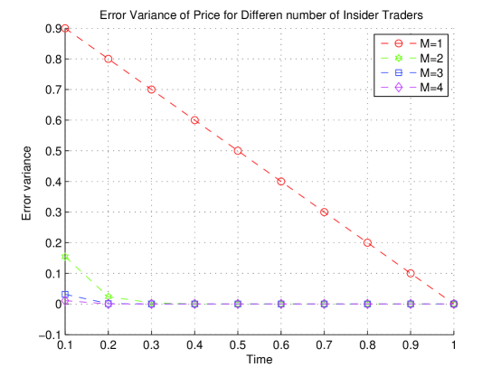
Figure 2: The number of auctions is fixed at $N=10$ and the error variance of price, $\Sigma_{n}$, is plotted for different values of $M$, $M=1$, $M=2$, $M=3$ or $M=4$.

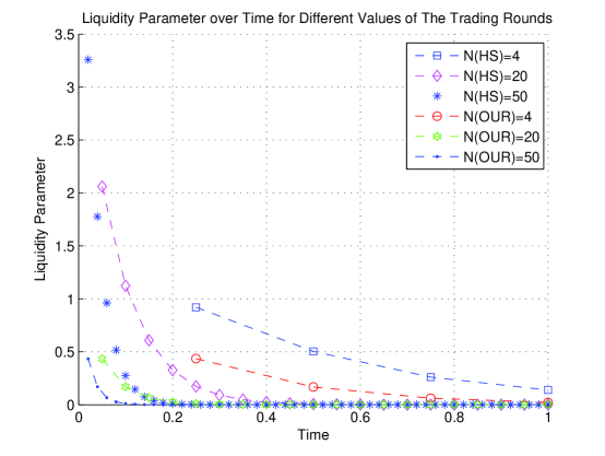
Figure 3: This figure contrasts the liquidity parameter $\lambda_{n}$, (i) when the insider must disclose each trade ex-post and (ii) when no such disclosures are made. The number of insiders is fixed at $M=2$ and the liquidity parameter at each auction is plotted for different value of $N$, $N=4$, $N=20$, $N=50$. $N(HS)$ in the figure means the $N$ in Holden and Subrahmanyam(1992) and $N(our)$ means the $N$ in our model.

Figure 4: This figure contrasts the error variance of price, $\Sigma_{n}$, in our model and in Holden and Subrahmanyam (1992)’s model, over time for different values of $N$, the number of trading rounds. The number of insiders is fixed at $M=2$ and the error variance of price at each auction is plotted for different value of $N$, $N=4$, $N=20$, $N=50$. $N(HS)$ in the figure means the $N$ in Holden and Subrahmanyam (1992) and $N(our)$ means the $N$ in our model.

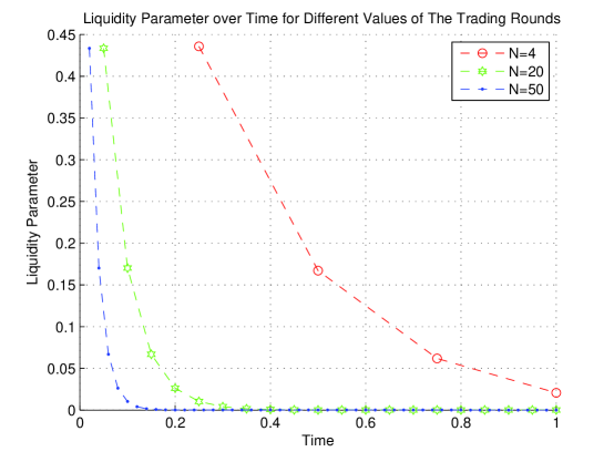
Figure 5: Liquidity parameter $\lambda_{n}$ over time for different values of $N$, the number of trading rounds. The number of insiders is fixed at $M=2$ and the liquidity parameter at each auction is plotted for different value of $N$, $N=4$, $N=20$, $N=40$.

Figure 6: The number of insiders is fixed at $M=2$ and the error variance of price, $\Sigma_{n}$, is plotted for different values of $N$, the number of auctions.

Figure $3$ and $4$ plot $\lambda_{n}$ and $\Sigma_{n}$ in our model and in Holden and Subrahmanyam (1992)’s, respectively, by holding constants $\Sigma_{0}=1$, $\sigma_{\mu}^{2}=1$, $M=2$ fixed and varying numbers of auctions, $N=4$, $N=20$, or $N=50.$ In order to see the behavior of $\lambda_{n}$ and $\Sigma_{n}$ in our model clearly, Figure $5$ and Figure $6$ again plot the liquidity parameter and the error variance for varying numbers of trading rounds, $N=4$, $N=20$, $N=50$, respectively.

Figure $3$ and Figure $4$ illustrate the contrast in the equilibria (i) when the insider must disclose each trade ex-post, and (ii) when no such disclosure are made. Figure $3$ illustrates that when the number of trading rounds fixed, the liquidity parameter $\lambda_{n}$ with public disclosure of insider trades is smaller than that without public disclosure. That is to say the adverse selection is low because of “public disclosure”. Also, as the number of trading rounds per unit time becomes larger, the $\lambda_{n}$ of Holden and Subrahmanyam (1992) in the initial periods become larger, but it is not the case in our model, which is potted clearly in Figure $5$. In Holden and Subrahmanyam (1992) the adverse selection (measured by $\lambda_{n}$) is high in the earlier periods because the information content of the order flow is high, and negligible in the later periods because market makers have very little to fear from traders that have already exploited most of their informational advantage. As the number of auctions is increased, trading becomes more concentrated at earlier auctions and hence there is greater adverse selection at these auctions. But under the requirement of “public disclosure”, market makers know that insiders may disclose their trading and may choose a mixed strategy to dissimulate their information, the adverse selection is the same at the initial auction even if the number of auctions increases.

Figure $4$ illustrates that as the number of trading rounds per unit time becomes very large, $\Sigma_{n}$ declines nearly to zero very rapidly both in the case of “public disclosure” and the case “without public disclosure”. And as the number of auctions increases, the speed with which they drop increases dramatically. But when the number of trading rounds fixed, the drop speed is faster under the requirement of “public disclosure”. That is to say, the “public disclosure” and aggressive competition among insiders lead to most of the private information to be incorporated into the price in the early auctions.

3 A convergence result–Near continuous trading

In this section, we will study the properties of the discrete model of sequential trading when the interval between auctions is vanishingly small, and analyze the behavior of the equilibrium when the market approaches continuous trading. Our main results, given in Theorem 3.1, concern the behavior of the equilibrium when the market approaches continuous trading. Unlike Back (1992) and Back, Cao, and Willard (2000) e.t.c formulating the continuous time model directly, we use the discrete models to approach continuous model, that is, use the discrete results Proposition 2.1 and then take the limit.

We assume there is $N$ auctions in the interval $[0,1]$, and the interval between auctions is the same.

In order to get the continuous result we first give the following key proposition, the proof of which is given in the appendix.

Proposition 3.1.

For any fixed $N$, the sequence $\{a_{n}\}$ described by the equation $(\ref{eq5.41})$ satisfy

$${}\frac{a_{n-1}^{2}}{a_{n}^{2}}\leq 1$$ (3.34)

where $1\leq n\leq N$.

The following theory is one of our main results:

Theorem 3.1.

As the interval between auctions in the discrete model becomes uniformly small, (i.e.$N\rightarrow+\infty$), the parameters characterized by the unique sequential auction equilibrium in Proposition 2.1 is convergent. More precisely, for any $t\in(0,1)$ , choose $N_{1}<N_{2}<\cdots<N_{j}<\cdots\rightarrow+\infty$, and satisfy $2+(1-t)N_{j}\leq(1-t)N_{j+1}<N_{j}-1,j=1,2,\cdots.$ For every $N_{j}$, let $n(N_{j})=[tN_{j}]$, $j=1,\cdots,$ where $[x]$ denote the integer part of $x$. When $j\rightarrow+\infty$, we have $\Sigma_{n(N_{j})}^{(N_{j})}\rightarrow\Sigma_{t}$, $\lambda_{n(N_{j})}^{(N_{j})}\rightarrow\lambda_{t}$, $\beta_{in(N_{j})}^{(N_{j})}\rightarrow\beta_{it}$,${\sigma_{z_{n(N_{j})}}^{(N_{j})}}^{2}\rightarrow\sigma_{z_{t}}^{2}$ and

(i)When $M=1$, $\Sigma_{t}$, $\lambda_{t}$, $\beta_{it}$ , $\sigma_{z_{t}}^{2}$ satisfy

$$\Sigma_{t}=(1-t)\Sigma_{0},~{}~{}~{}~{}\lambda_{t}=0,$$

$$\beta_{it}=0~{}~{}(i=1),~{}~{}~{}~{}~{}\sigma_{z_{t}}^{2}=\sigma_{\mu}^{2}.$$

(ii) When $M\geq 2$, $\Sigma_{n(N_{j})}^{(N_{j})}$ satisfies

$$\exp\left\{[tN_{j}]\log\left(1-\frac{A}{M}\right)+o(N_{j})\right\}\leq\frac{\Sigma_{n(N_{j})}^{(N_{j})}}{\Sigma_{0}}\leq\exp\left\{[tN_{j}]\log\left(1-\frac{A}{M}\right)\right\}$$ (3.35)

i.e. $\frac{\Sigma_{n(N_{j})}^{N_{j}}}{\Sigma_{0}}\approx\exp\left\{[tN_{j}]\log\left(1-\frac{A}{M}\right)\right\}$, and

$$\lim_{N_{j}\rightarrow+\infty}\lambda_{1}^{(N_{j})}=\frac{\sqrt{\Sigma_{0}}A}{(M+1)\sigma_{\mu}},$$ (3.36)

$$\lim_{N_{j}\rightarrow+\infty}\beta_{1}^{(N_{j})}=\frac{A\sigma_{\mu}}{M\sqrt{\Sigma_{0}}},$$ (3.37)

furthermore, $\Sigma_{t}$, $\lambda_{t}$, $\beta_{it}$ , $\sigma_{z_{t}}^{2}$ satisfy

$$\Sigma_{t}=0,~{}~{}~{}~{}~{}\lambda_{t}=0,$$

$$\beta_{it}=+\infty,~{}~{}~{}\sigma_{z_{t}}^{2}=\frac{\sigma_{\mu}^{2}}{M}(1-\frac{A}{M}),$$

where $A$ is the unique root of $f(x)\doteq(M-1)^{2}x^{3}-4(M+1)(M-1)^{2}x^{2}+(M^{2}-1)(6M^{2}-4)x+(M+1)^{2}(4M^{2}-3M^{3})=0$ in $(0,M)$.

Proof.

See the Appendix. ∎

Theorem 3.1 implies that, when $M=1$, the speed of insiders’ information incorporated into the price is a linear function of the time $t$. This is a limiting result of Hudart, Hughes and Levine (2001). When $M\geq 2$ , the speed of the insiders’ information is not incorporated into the price is approximate a exponential function of the time $[tN_{j}]$. When $j\rightarrow+\infty$, $\Sigma_{t}=0$, $\lambda_{t}=0$ for all $t\in(0,1),$ that is to say, as the number of auctions goes to infinity, all information is revealed immediately and the market depth goes to infinity immediately. These results described in Theorem 3.1 are consistent with the results numerical illustrated in section $2$.

But another class of limits (i.e. $\lim_{N_{j}\rightarrow+\infty}\lambda_{1}^{(N_{j})}=\frac{\sqrt{\Sigma_{0}}A}{(M+1)\sigma_{\mu}}$ and $\lim_{N_{j}\rightarrow+\infty}\beta_{1}^{(N_{j})}=\frac{A\sigma_{\mu}}{M\sqrt{\Sigma_{0}}}$) show that, as the total number of auction goes to infinity, the market depth at the first auction is a constant, and the trading intensity is also a constant. However, Holden and Subrahmanyam (1992) find that the market depth at the first auction goes to zero and trading intensity $\beta_{1}$ goes to infinity. The intuition for the contrast is that “public disclosure” enable higher adverse selection in the market.

4 Conclusion

In this paper, we consider a model in which there are at least two informed traders in the market, with the requirement that insiders publicly disclose their stock trades after the fact but not verification by others. In equilibrium, the “public disclosure” and “competition among insiders”assumptions have great effects on each insider’s trading intensity, the market depth and the effectiveness of the price.

We have shown that the contrast between our results and those of Hudart, Hughes and Levine (2001) and the contrast between our results and those of Holden and Subrahmanyan (1992) are far from trivial. In particular, in our model, as the interval between auctions approaches zero, the market approaches the perfectly competitive outcome of full information revelation and infinite market depth almost immediately, in contrast to the case of a monopolist considered by Hudart, Hughes and Levine (2001), wherein market depth is constant at all times and information is revealed at a linear speed. Moreover, in the two-period trading, the market depth of the first auction in our model is smaller than Hudart, Hughes and Levine (2001)’s when the number of insiders is less than $5$, and the opposite conclusion holds if the number of insiders is more than $5$. That is to say, whether market makers set the marginal cost of the first period traders lower or higher depends on the number of insiders. If the number of insiders is big enough (bigger than $5$), the adverse selection becomes small. Comparing with Holden and Subrahmanyan(1992)’s model, each insider plays a mixed strategy in every round except the last one, because of the existence of “public disclosure”, leading to the accelerated price discovery and higher market depths. Furthermore, in the sequential auction equilibrium, market depths become infinite and all private information is revealed immediately when the time interval between auctions approaches zero. The speed of the revelation is faster than that of Holden and Subrahmanyan (1992), and we give the exact speed of the revelation in Theorem 3.1.

Moreover, we give the near-continuous trading results by starting with discrete time and then taking the limit, rather than formulating the model directly in continuous time. We find that the speed of insiders’ information incorporated into the price is a linear function of the time $t$ ($t\in(0,1)$) when there is one insider in the market. However, if there are more than two insiders, the speed of the insiders’ information is not incorporated into the price is approximate a exponential function of the time $[tN]$, where $t\in(0,1)$ is the time and $N$ is the total number of auctions in $(0,1).$ That is to say, when there are more than two insiders in the market all information is revealed immediately and the market depth goes to infinity immediately as the number of auctions goes to infinite where the market is strong-form efficient. An interesting find is that as the total number of auction goes to infinity, the market depth and the trading intensity at the first auction are all constants while Holden and Subrahmanyam (1992) find that the market depth at the first auction goes to zero and the trading intensity of the first period goes to infinity. The intuition for the contrast is that “public disclosure” enable less adverse selection in the market.

Our results have two important implications. Firstly, under the requirement of “public disclosure”, the market can be close to strong-form efficiency even when the presence of just two noncooperative privately informed traders is assumed. Secondly, despite being close to efficiency, the market depth at the first auction is a constant. These implications are in sharp contrast to previous literature.

Our model not only shows that insiders are able to profit from long-lived private information even though they must disclose their trades at the end of each trading, but also can be applied to lots of intra-day phenomena, such as adverse selection problem and so on.

5 Appendix

We first recall a well-known regression result which will be used.

Lemma 5.1.

Let $X_{1}$ and $X_{2}$ be two normal random vectors, $\left(\begin{array}[]{c}X_{1}\\ X_{2}\end{array}\right)\sim N(\mu,\Sigma)$ with $\mu=\left(\begin{array}[]{c}\mu_{1}\\ \mu_{2}\end{array}\right)$, $\Sigma=\left(\begin{array}[]{cc}\Sigma_{11}&\Sigma_{12}\\ \Sigma_{21}&\Sigma_{22}\end{array}\right)$. Then the random variable $X_{1}$ conditional on $X_{2}$ has a normal distribution. More precisely ,

$$E[X_{1}|X_{2}]=\mu_{1}+\Sigma_{12}\Sigma_{22}^{-1}(X_{2}-\mu_{2}),~{}~{}~{}~{}Var(X_{1}|X_{2})=\Sigma_{11}-\Sigma_{12}\Sigma_{22}^{-1}\Sigma_{21}.$$

Proof of Proposition 1.1: Let $N$ in Proposition $1$ of Holden and Subrahmanyam (1992) equal $2$ and $\Delta t_{n}$ $(n=1,\cdots,N.)$ equal $1$, we have the following relationships :

$${}\alpha_{1}=\frac{1-\alpha_{2}\lambda_{2}}{\lambda_{2}[M(1-2\alpha_{2}\lambda_{2})+1]^{2}},$$ (5.38)

$${}\alpha_{2}=0,$$ (5.39)

$${}\beta_{1}=\frac{1-2\alpha_{1}\lambda_{1}}{\lambda_{1}[M(1-2\alpha_{1}\lambda_{1})+1]},$$ (5.40)

$${}\beta_{2}=\frac{1}{\lambda_{2}(M+1)},$$ (5.41)

$${}\lambda_{1}=\frac{M\beta_{1}\Sigma_{1}}{\sigma_{\mu}^{2}},$$ (5.42)

$${}\lambda_{2}=\frac{1}{\sigma_{\mu}}\left(\frac{M\Sigma_{2}}{M+1}\right)^{\frac{1}{2}},$$ (5.43)

$${}\Sigma_{2}=(1-M\beta_{2}\lambda_{2})\Sigma_{1},$$ (5.44)

$${}\Sigma_{1}=(1-M\beta_{1}\lambda_{1})\Sigma_{0}.$$ (5.45)

Let $k\doteq\frac{\lambda_{1}}{\lambda_{2}}$, from (5.38) and (5.39) we get

$${}\alpha_{1}=\frac{1}{\lambda_{2}(M+1)^{2}}.$$ (5.46)

Combining (5.40) and (5.46), we get the expression of $\beta_{1}$

$$\beta_{1}=\frac{1-\frac{2k}{(M+1)^{2}}}{\lambda_{1}[M(1-\frac{2k}{(M+1)^{2}})+1]}=\frac{(M+1)^{2}-2k}{\lambda_{1}[(M+1)^{3}-2kM]}.$$

The expression of $\beta_{1}$ and (5.45) imply

$${}\Sigma_{1}=\left(1-\frac{M(M+1)^{2}-2kM}{(M+1)^{3}-2kM}\right)\Sigma_{0}=\frac{(M+1)^{2}\Sigma_{0}}{(M+1)^{3}-2kM}.$$ (5.47)

(5.41),(5.44) and (5.47) give:

$${}\Sigma_{2}=\frac{1}{M+1}\Sigma_{1}=\frac{(M+1)\Sigma_{0}}{(M+1)^{3}-2kM}.$$ (5.48)

(5.42) and (5.47) imply:

$${}\lambda_{1}^{2}=\frac{M(M+1)^{2}[(M+1)^{2}-2k]\Sigma_{0}}{[(M+1)^{3}-2kM]^{2}\sigma_{\mu}^{2}}.$$ (5.49)

Combining (5.43) and (5.48)

$${}\lambda_{2}^{2}=\frac{1}{\sigma_{\mu}^{2}}\frac{M\Sigma_{0}}{(M+1)^{3}-2kM.}$$ (5.50)

From the above two equations it is easy to get

$$k^{2}\doteq\frac{\lambda_{1}^{2}}{\lambda_{2}^{2}}=\frac{(M+1)^{2}[(M+1)^{2}-2k]}{(M+1)^{3}-2kM}.$$ (5.51)

The polynomial $2Mk^{3}-(M+1)^{3}k^{2}-2(M+1)^{2}k+(M+1)^{4}=0$ has three roots, but from the second order condition of Proposition $1$ in Holden and Subrahmanyam (1992), $\lambda_{1}>0$, $\lambda_{2}>0$. It is easy to show that the polynomial only has one root satisfying conditions $\lambda_{1}>0$ and $\lambda_{2}>0$.

Proof of Proposition 1.3:   From Proposition $2$ of Hudart, Hughes and Levine (2001), we get

$$\bar{\lambda}_{1}=\bar{\lambda}_{2}=\frac{1}{2\sigma_{\mu}}\sqrt{\frac{\Sigma_{0}}{2}},$$

$$\bar{\beta}_{1}=\frac{\sigma_{\mu}}{\sqrt{2\Sigma_{0}}},~{}~{}~{}\bar{\beta}_{2}=\frac{\sqrt{2}\sigma_{\mu}}{\sqrt{\Sigma_{0}}}$$

$$\bar{\Sigma}_{1}=\frac{1}{2}\Sigma_{0}.$$

So ,

$$\frac{\lambda_{1}}{\bar{\lambda}_{1}}=\sqrt{\frac{8M^{3}}{4+M^{2}(M+1)^{2}}}=\left\{\begin{array}[]{c}>1,\ \ \ 2\leq M\leq 5\\ <1,\ \ \ M>5\end{array}\right.,$$

$$\frac{\lambda_{2}}{\bar{\lambda}_{2}}=\frac{4}{(M+1)^{2}}\sqrt{\frac{2M}{[4+M^{2}(M+1)^{2}]}}<1,$$

$$\frac{\beta_{i1}}{\bar{\beta}_{1}}=(M+1)\sqrt{\frac{2M}{4+M^{2}(M+1)^{2}}}<1,$$

$$\frac{\beta_{i2}}{\bar{\beta}_{2}}=\sqrt{\frac{4+M^{2}(M+1)^{2}}{8M}}>1,$$

$$\frac{\Sigma_{1}}{\bar{\Sigma}_{1}}=\frac{8}{4+M^{2}(M+1)^{2}}<1.$$

Proof of Proposition 1.4: Let the $M$ in Proposition 1.1 equal $2$, we have

$$\tilde{\lambda}_{1}=\frac{\sqrt{2\Sigma_{0}(1-\frac{2k}{9})}}{\sigma_{\mu}(3-\frac{4k}{9})},~{}~{}~{}\tilde{\lambda}_{2}=\frac{1}{3\sigma_{\mu}}\sqrt{\frac{2\Sigma_{0}}{3-\frac{4k}{9}}},$$

$$\tilde{\beta}_{1}=\frac{1-\frac{2k}{9}}{\tilde{\lambda}_{1}(3-\frac{4k}{9})}=\sigma_{\mu}\sqrt{\frac{1-\frac{2k}{9}}{2\Sigma_{0}}},~{}~{}~{}\tilde{\beta}_{2}=\frac{1}{3\tilde{\lambda}_{2}}=\sigma_{\mu}\sqrt{\frac{3-\frac{4k}{9}}{2\Sigma_{0}}},$$

$$\tilde{\Sigma}_{1}=\frac{\Sigma_{0}}{3-\frac{4k}{9}},$$

and the $k\doteq\frac{\lambda_{1}}{\lambda_{2}}$ satisfies: $4k^{3}-27k^{2}-18k+81=0$, so $k=6.9790,-1.8218$, or $1.5927.$ By the second order condition we have $\lambda_{1}>0$, so $k$ must satisfy $0<k<4.5$. So $k=1.5927$. Let the $M$ in Proposition 1.2 equal $2$, we have

$$\lambda_{1}=\frac{\sqrt{\Sigma_{0}}}{3\sigma_{\mu}\sqrt{5}},~{}~{}~{}\lambda_{2}=\frac{\sqrt{\Sigma_{0}}}{3\sigma_{\mu}\sqrt{5}},$$

$$\beta_{i1}=\frac{3\sigma_{\mu}\sqrt{5}}{10\sqrt{\Sigma_{0}}},~{}~{}~{}\beta_{i2}=\frac{\sigma_{\mu}\sqrt{5}}{\sqrt{\Sigma_{0}}},$$

$$\Sigma_{1}=\frac{1}{10}\Sigma_{0}.$$

So, it is easy to get

$$\frac{\lambda_{1}}{\tilde{\lambda}_{1}}=\frac{\sqrt{\Sigma_{0}}}{\sigma_{\mu}\sqrt{5}}\times\frac{\sigma_{\mu}(3-\frac{4k}{9})}{\sqrt{2\Sigma_{0}(1-\frac{2k}{9})}}\approx\frac{2.39}{\sqrt{6.5}}<1,$$

$$\frac{\lambda_{2}}{\tilde{\lambda}_{2}}=\frac{\sqrt{\Sigma_{0}}}{3\sigma_{\mu}\sqrt{5}}\times\frac{3\sigma_{\mu}(3-\frac{4k}{9})}{\sqrt{2\Sigma_{0}}}\approx\frac{\sqrt{2.3}}{\sqrt{10}}<1,$$

$$\frac{\beta_{i1}}{\tilde{\beta}_{1}}=\frac{3\sigma_{\mu}\sqrt{5}}{10\sqrt{\Sigma_{0}}}\times\frac{\sqrt{2\Sigma_{0}}}{\sigma_{\mu}\sqrt{1-\frac{2k}{9}}}\approx\frac{3}{\sqrt{7.4}}>1,$$

$$\frac{\beta_{i2}}{\tilde{\beta}_{2}}=\frac{\sigma_{\mu}\sqrt{5}}{\sqrt{\Sigma_{0}}}\times\frac{\sqrt{2\Sigma_{0}}}{\sigma_{\mu}\sqrt{3-\frac{4k}{9}}}\approx\frac{\sqrt{10}}{\sqrt{2.3}}>1.$$

Proof of Proposition 2.1: Applying the principal of backward induction, we can write the insider $i$’s last period ($N$th period) optimization problem for given $x_{i1},\cdots,x_{i,N-1},p_{1}^{*},\cdots,p_{N-1}^{*}$ as $x_{iN}\in arg\max_{x}E[x(v-p_{N})|x_{j1},\cdots,x_{j,N-1},1\leq j\leq M,p_{1}^{*},\cdots,p_{N-1}^{*},v]$, where

$$E[x(v-p_{N})|x_{j1},\cdots,x_{j,N-1},1\leq j\leq M,p_{1}^{*},\cdots,p_{N-1}^{*},v]$$

$$= E[x(v-p_{N-1}^{*}-\lambda_{N}x-\lambda_{N}(M-1)\bar{x}_{iN})|x_{j1},\cdots,x_{j,N-1},1\leq j\leq M,p_{1}^{*},\cdots,p_{N-1}^{*},v]$$

$$= x[v-p_{N-1}^{*}-\lambda_{N}x-\lambda_{N}(M-1)\bar{x}_{iN}],$$

in the above $\bar{x}_{iN}$ represents the particular informed trader’s conjecture of the average of the other informed traders’ strategies, i.e. $\bar{x}_{iN}=\frac{1}{M-1}E[\sum_{j\neq i}x_{jN}|x_{j1},\cdots,x_{j,N-1},1\leq j\leq M,p_{1}^{*},\cdots,p_{N-1}^{*},v]$. By the first order condition we can have

$$v-p_{N-1}^{*}-2\lambda_{N}x_{iN}-\lambda_{N}(M-1)E[\sum_{j\neq i}x_{jN}|x_{j1},\cdots,x_{j,N-1},1\leq j\leq M,p_{1}^{*},\cdots,p_{N-1}^{*},v]=0.$$

By the theory of solving linear equations, we know $x_{1N}=x_{2N}=\cdots=x_{MN}$, $\bar{x}_{iN}=x_{iN}$, and $x_{iN}=\frac{1}{(M+1)\lambda_{N}}(v-p_{N-1}^{*})$. So,

$$\beta_{iN}=\frac{1}{(M+1)\lambda_{N}},$$

and

$$E(\pi_{iN}|x_{i1},\cdots,x_{i,N-1},p_{1}^{*},\cdots,p_{N-1}^{*},v)$$

$$= \max_{x}E[x(v-p_{N})|x_{i1},\cdots,x_{i,N-1},p_{1}^{*},\cdots,p_{N-1}^{*},v]$$

$$= x_{iN}(v-p_{N-1}^{*}-\lambda_{N}Mx_{iN})$$

$$= \frac{1}{(M+1)\lambda_{N}}(v-p_{N-1}^{*})[v-p_{N-1}^{*}-\frac{M}{(M+1)}(v-p_{N-1}^{*})]$$

$$= \frac{1}{(M+1)^{2}\lambda_{N}}(v-p_{N-1}^{*})^{2},$$

which implies $\alpha_{N-1}=\frac{1}{(M+1)^{2}\lambda_{N}},\delta_{N-1}=0$. By the market efficient condition we can have $\lambda_{N}=\frac{\beta_{iN}\Sigma_{N-1}}{\beta_{iN}^{2}\Sigma_{N-1}+\sigma_{\mu}^{2}}$, i.e., $\lambda_{N}=\frac{\sqrt{M\Sigma_{N-1}}}{(M+1)\sigma_{\mu}}$.

Now make the inductive hypothesis that for constants $\alpha_{n}$ and $\delta_{n}$

$${}E(\pi_{i,n+1}|p_{1}^{*},\cdots,p_{n}^{*},p_{1},\cdots,p_{n},v)=\alpha_{n}(v-p_{n}^{*})^{2}+\delta_{n}.$$ (5.52)

Since $\pi_{in}$ is given recursively by $\pi_{in}=(v-p_{n})x_{in}+\pi_{i,n+1}$, we obtain

$$E(\pi_{i,n}|p_{1}^{*},\cdots,p_{n-1}^{*},p_{1},\cdots,p_{n-1},v)$$ (5.53)

$$= \max_{x}E\{(v-p_{n})x+\alpha_{n}(v-p_{n}^{*})^{2}+\delta_{n}|p_{1}^{*},\cdots,p_{n-1}^{*},p_{1},\cdots,p_{n-1},v\}.$$

In a linear equilibrium, $p_{n}$ and $p_{n}^{*}$ are given by

$${}p_{n}=p_{n-1}^{*}+\lambda_{n}y_{n},$$ (5.54)

$$p_{n}^{*}=p_{n-1}^{*}+\gamma_{n}x_{n}.$$ (5.55)

Now, $x_{n}$ can be written as $x_{in}+(M-1)\bar{x}_{in}$, where $\bar{x}_{in}$ represents the particular informed trader’s conjecture of the average of the other informed traders’ strategies, so we have

$$E(\pi_{i,n}|p_{1}^{*},\cdots,p_{n-1}^{*},p_{1},\cdots,p_{n-1},v)$$ (5.56)

$$= \max_{x}E\{(v-p_{n-1}^{*}-\lambda_{n}y_{n})x+\alpha_{n}(v-p_{n-1}^{*}-\gamma_{n}x_{n})^{2}+\delta_{n}|p_{1}^{*},\cdots,p_{n-1}^{*},p_{1},\cdots,p_{n-1},v\}$$

$$= \max_{x}\{(v-p_{n-1}^{*}-\lambda_{n}x-\lambda_{n}(M-1)\bar{x}_{in})x+\alpha_{n}(v-p_{n-1}^{*}-\gamma_{n}x-\gamma_{n}(M-1)\bar{x}_{in})^{2}$$

$$+\delta_{n}\}.$$

By the first order condition, we can get

$${}v-p_{n-1}^{*}-2\lambda_{n}x_{in}-\lambda_{n}(M-1)\bar{x}_{in}-2\gamma_{n}\alpha_{n}[v-p_{n-1}^{*}-\gamma_{n}x_{in}-\gamma_{n}(M-1)\bar{x}_{in}]=0,$$ (5.57)

and the second order condition is

$${}\lambda_{n}\geq\frac{2\gamma_{n}^{2}\alpha_{n}M}{(M+1)}.$$ (5.58)

Using the strategy symmetry for each insider again, we have $\bar{x}_{in}=x_{in}$. $(\ref{eq5.19})$ can be rewritten as

$${}(1-2\gamma_{n}\alpha_{n})(v-p_{n-1}^{*})+[2\gamma_{n}^{2}\alpha_{n}M-(M+1)\lambda_{n}]x_{in}=0.$$ (5.59)

Since the insider must be willing to play a mixed strategy, $x_{in}=\beta_{in}(v-p_{n-1}^{*})+z_{n}$, and $z_{n}$ is independent with $v-p_{n-1}^{*}$, we have the following two equations by substituting the expression of $x_{in}$ into $(\ref{eq5.21})$,

$${}1-2\gamma_{n}\alpha_{n}=0,$$ (5.60)

$${}2\gamma_{n}^{2}\alpha_{n}M-(M+1)\lambda_{n}=0.$$ (5.61)

Using $x_{in}=\beta_{in}(v-p_{n-1}^{*})+z_{n}$ again, we get

$$E(\pi_{i,n}|p_{1}^{*},\cdots,p_{n-1}^{*},p_{1},\cdots,p_{n-1},v)$$ (5.62)

$$= E\{[v-p_{n-1}^{*}-\lambda_{n}M\beta_{in}(v-p_{n-1}^{*})-\lambda_{n}Mz_{n}-\lambda_{n}\mu_{n}][\beta_{in}(v-p_{n-1}^{*})+z_{n}]$$

$$+\alpha_{n}[v-p_{n-1}^{*}-\gamma_{n}M\beta_{in}(v-p_{n-1}^{*})-\gamma_{n}Mz_{n}]^{2}+\delta_{n}|p_{1}^{*},\cdots,p_{n-1}^{*},p_{1},\cdots,p_{n-1},v\}$$

$$= [\beta_{in}(1-\lambda_{n}M\beta_{in})+\alpha_{n}(1-\gamma_{n}M\beta_{in})^{2}](v-p_{n-1}^{*})^{2}+\alpha_{n}\gamma_{n}^{2}M^{2}\sigma_{z_{n}}^{2}-\lambda_{n}M\sigma_{z_{n}}^{2}+\delta_{n},$$

so,

$${}\alpha_{n-1}=\beta_{in}(1-\lambda_{n}M\beta_{in})+\alpha_{n}(1-\gamma_{n}M\beta_{in})^{2},$$ (5.63)

$$\delta_{n-1}=\alpha_{n}\gamma_{n}^{2}M^{2}\sigma_{z_{n}}^{2}-\lambda_{n}M\sigma_{z_{n}}^{2}+\delta_{n}.$$

By (5.60) and (5.61) we get

$$\delta_{n-1}= \frac{M-1}{2(M+1)}M^{2}\gamma_{n}\sigma_{z_{n}^{2}}+\delta_{n},$$ (5.64)

(5.63) and (5.64) are just (2.26) and (2.27).

Now by the market efficient condition we get

$$p_{n}-p_{n-1}^{*}= E(v-p_{n-1}^{*}|y_{1},\cdots,y_{n},p_{1}^{*},\cdots,p_{n-1}^{*},p_{1},\cdots,p_{n-1})$$ (5.65)

$$= E[v-p_{n-1}^{*}|M\beta_{in}(v-p_{n-1}^{*})+Mz_{n}+\mu_{n}].$$

By Lemma 5.1 we have

$${}\lambda_{n}=\frac{M\beta_{in}\Sigma_{n-1}}{M^{2}\beta_{in}^{2}\Sigma_{n-1}+M^{2}\sigma_{z_{n}}^{2}+\sigma_{\mu}^{2}}.$$ (5.66)

Using the same method, we get the expression of $\gamma_{n}$ as

$${}\gamma_{n}=\frac{M\beta_{in}\Sigma_{n-1}}{M^{2}\beta_{in}^{2}\Sigma_{n-1}+M^{2}\sigma_{z_{n}}^{2}}.$$ (5.67)

From the equation (5.60) and (5.61) it is easy to get that $\lambda_{n}=\frac{M\gamma_{n}}{M+1}$. Combining the equation (5.66) and (5.67), we have

$${}M^{2}\beta_{in}^{2}\Sigma_{n-1}+M^{2}\sigma_{z_{n}}^{2}=M\sigma_{\mu}^{2}.$$ (5.68)

Now we consider $\Sigma_{n}$, the measure of the informativeness of price,

$$\Sigma_{n}= Var(v|x_{1},\cdots,x_{n},p_{1},\cdots,p_{n-1},p_{1}^{*},\cdots,p_{n-1}^{*})$$ (5.69)

$$= Var(v-p_{n-1}^{*}|M\beta_{in}(v-p_{n-1}^{*})+Mz_{n}),$$

using Lemma 5.1 again, we have

$$\Sigma_{n}= \Sigma_{n-1}-\frac{M^{2}\beta_{in}^{2}\Sigma_{n-1}^{2}}{M^{2}\beta_{in}^{2}\Sigma_{n-1}+M^{2}\sigma_{z_{n}}^{2}}$$ (5.70)

$$= \Sigma_{n-1}-\frac{(M+1)^{2}}{M}\lambda_{n}^{2}\sigma_{\mu}^{2}.$$

The equation $\alpha_{n}=\frac{1}{2\gamma_{n}}=\frac{M}{2(M+1)\lambda_{n}}$ implies

$${}\lambda_{n}=\frac{M}{2(M+1)\alpha_{n}}.$$ (5.71)

Now we only need to prove the expressions of $\beta_{in}$ and $\sigma_{z_{n}}^{2}$.

(5.66) and (5.68) yield $\lambda_{n}=\frac{M\beta_{in}\Sigma{n-1}}{(M+1)\sigma_{\mu}^{2}}$, thus

$${}\beta_{in}=\frac{\lambda_{n}(M+1)\sigma_{\mu}^{2}}{M\Sigma_{n-1}}.$$ (5.72)

Combining (5.68) and (5.72), we get the expression of $\sigma_{z_{n}}^{2}$ as

$${}\sigma_{z_{n}}^{2}=\frac{1}{M}\left(\sigma_{\mu}^{2}-\frac{\lambda_{n}^{2}(M+1)^{2}\sigma_{\mu}^{4}}{M\Sigma_{n-1}}\right).$$ (5.73)

Next we prove that the difference equation system consisted by equation (5.63), (5.64), (5.70), (5.71), (5.72) and (5.73) has a unique solution. We suppose that $\lambda_{n}=\frac{\sqrt{\Sigma_{n-1}}}{(M+1)\sigma_{\mu}}a_{n}$, where $a_{n}$ is a function of $n$. In turn, (5.70) reduces to

$${}\Sigma_{n}=\left(1-\frac{a_{n}^{2}}{M}\right)\Sigma_{n-1}.$$ (5.74)

From this equation, we have $0<a_{n}<\sqrt{M}$ ($n=1,\cdots,N-1$), and $a_{N}=\sqrt{M}$. Then , it is easy to get

$${}\alpha_{n}=\frac{M}{2(M+1)\lambda_{n}}=\frac{M\sigma_{\mu}}{2\sqrt{\Sigma_{n-1}a_{n}}},$$ (5.75)

$${}\beta_{in}=\frac{a_{n}\sigma_{\mu}}{M\sqrt{\Sigma_{n-1}}}.$$ (5.76)

Then $(\ref{eq5.25})$ yields

$${}\frac{M}{2a_{n-1}\sqrt{\Sigma_{n-2}}}=\frac{2(M+1)(1-M)a_{n}^{2}+(M-1)a_{n}^{4}+M^{2}(M+1)}{2M(M+1)a_{n}\sqrt{\Sigma_{n-1}}}.$$ (5.77)

Substituting $\Sigma_{n-1}=\left(1-\frac{a_{n-1}^{2}}{M}\right)\Sigma_{n-2}$ into the above equation we get

$${}\frac{\sqrt{M(M-a_{n-1}^{2})}}{2a_{n-1}}=\frac{(1-M)a_{n}}{M}+\frac{(M-1)a_{n}^{3}}{2M(M+1)}+\frac{M}{2a_{n}}.$$ (5.78)

Because $0<a_{n}<\sqrt{M}$($n=1,\cdots,N-1$), $a_{N}=\sqrt{M}$, the above equation is equivalent to the following equation

$${}a_{n-1}=\left(\frac{M^{4}(M+1)^{2}a_{n}^{2}}{M^{3}(M+1)^{2}a_{n}^{2}+[2(M+1)(1-M)a_{n}^{2}+(M-1)a_{n}^{4}+M^{2}(M+1)]^{2}}\right)^{\frac{1}{2}}.$$ (5.79)

From this equation we can know that every $a_{n}$ exists and is unique for given $a_{N}=\sqrt{M}$. Therefore, the difference equation system has a unique solution.

Proof of Proposition 3.1: By equation $(\ref{eq5.41})$, we have

$${}\frac{a_{n-1}^{2}}{a_{n}^{2}}=\frac{M^{4}(M+1)^{2}}{M^{3}(M+1)^{2}a_{n}^{2}+[2(M+1)(1-M)a_{n}^{2}+(M-1)a_{n}^{4}+M^{2}(M+1)]^{2}}.$$ (5.80)

Because

$$M^{3}(M+1)^{2}a_{n}^{2}+[2(M+1)(1-M)a_{n}^{2}+(M-1)a_{n}^{4}+M^{2}(M+1)]^{2}$$ (5.81)

$$= M^{4}(M+1)^{2}+(M+1)^{2}(4M^{2}-3M^{3})a_{n}^{2}+2M^{2}(M^{2}-1)a_{n}^{4}$$

$$+[2(M+1)(1-M)a_{n}^{2}+(M-1)a_{n}^{4}]^{2}.$$

Let $b_{n}=a_{n}^{2}$, we have

$${}\frac{a_{n-1}^{2}}{a_{n}^{2}}=\frac{M^{4}(M+1)^{2}}{M^{4}(M+1)^{2}+F(b_{n})},$$ (5.82)

where $F(x)$ satisfies

$${}F(x)= x\left\{(M+1)^{2}(4M^{2}-3M^{3})+2M^{2}(M^{2}-1)x+x[2(M+1)(1-M)+(M-1)ax]^{2}\right\}$$ (5.83)

$$= x\left\{(M-1)^{2}x^{3}-4(M+1)(M-1)^{2}x^{2}+(M^{2}-1)(6M^{2}-4)x+(M+1)^{2}(4M^{2}-3M^{3})\right\}.$$

It is easy to get that $F(M)=4M^{2}$.

Now, for any fixed $N$, we prove $\frac{a_{n-1}^{2}}{a_{n}^{2}}\leq 1$. Let

$${}f(x)\doteq(M-1)^{2}x^{3}-4(M+1)(M-1)^{2}x^{2}+(M^{2}-1)(6M^{2}-4)x+(M+1)^{2}(4M^{2}-3M^{3}),$$ (5.84)

so

$${}f^{\prime}(x)=3(M-1)^{2}x^{2}-8(M+1)(M-1)^{2}x+(M^{2}-1)(6M^{2}-4).$$ (5.85)

Let $f^{\prime}(x)=0$, since the $\Delta$ of the above quadratic equation is

$${}\Delta= 64(M+1)^{2}(M-1)^{4}-12(M-1)^{2}(M^{2}-1)(6M^{2}-4)$$ (5.86)

$$=8(M-1)^{2}(M^{2}-1)(-M^{2}-2)<0,$$

so for any $x$, $f(x)$ is increasing. On the other hand, $f(0)=(M+1)^{2}(4M^{2}-3M^{3})<0$, $f(M)=4M>0$, so $f(x)$ have a unique solution in $(0,M)$, we denote the solution is $A$.

If for any $n,1\leq n\leq N-1$, $a_{n}^{2}\in[A,M)$, by

$${}\frac{a_{n-1}^{2}}{a_{n}^{2}}=\frac{M^{4}(M+1)^{2}}{M^{4}(M+1)^{2}+a_{n}^{2}f(a_{n}^{2})},$$ (5.87)

and $f(a_{n}^{2})>0$, we have $\frac{a_{n-1}^{2}}{a_{n}^{2}}\leq 1$, then the proposition is proved.

So we only need to prove that for any $n,1\leq n\leq N-1$, $a_{n}^{2}\in[A,M)$. In order to prove this conclusion, we fist give the following proposition.

Proposition 5.1.

The real root of $f(x)=0$, denoted by $A$, satisfies

$$A\in\left(M-\frac{4M}{(M-1)(M^{3}+3M^{2}+4M-4)},M-\frac{4M}{M^{2}(M+1)^{2}+4}\right).$$ (5.88)

Proof.

: From $a_{N}=\sqrt{M}$ and equation $(\ref{eq5.41})$, we have

$${}a_{N-1}=\sqrt{\frac{M^{3}(M+1)^{2}}{M^{2}(M+1)^{2}+4}}.$$ (5.89)

In order to get the range of $A$, we first compute $f(M-\varepsilon)$, where $0<\varepsilon<M$.

$${}f(M-\varepsilon)= (M-1)^{2}(M-\varepsilon)^{3}-4(M+1)(M-1)^{2}(M-\varepsilon)^{2}+$$ (5.90)

$$(M^{2}-1)(6M^{2}-4)(M-\varepsilon)+(M+1)^{2}(4M^{2}-3M^{3})$$

$$= -(M-1)^{2}\varepsilon^{3}-(M-1)^{2}(M+4)\varepsilon^{2}-$$

$$(M-1)(M^{3}+3M^{2}+4M-4)\varepsilon+4M,$$

so from the above equation we have

$${}f\left(M-\frac{4M}{(M-1)(M^{3}+3M^{2}+4M-4)}\right)<0,$$ (5.91)

i.e.

$${}A>M-\frac{4M}{(M-1)(M^{3}+3M^{2}+4M-4)}.$$ (5.92)

On the other hand, $(\ref{eq6.10})$ implies

$$f\left(M-\frac{4M}{M^{2}(M+1)^{2}+4}\right)$$ (5.93)

$$= \frac{1}{[M^{2}(M+1)^{2}+4]^{3}}\{-64M^{3}(M-1)^{2}-16M^{2}(M-1)^{2}(M+4)[M^{2}(M+1)^{2}+4]$$

$$+32M^{2}[M^{2}(M+1)^{2}+4]^{2}\}$$

$$= \frac{32M^{2}}{[M^{2}(M+1)^{2}+4]}-\frac{16M^{2}(M-1)^{2}(M+4)}{[M^{2}(M+1)^{2}+4]^{2}}-\frac{64M^{3}(M-1)^{2}}{[M^{2}(M+1)^{2}+4]^{3}},$$

and

$$\frac{M^{3}(M+1)^{2}}{M^{2}(M+1)^{2}+4}f\left(M-\frac{4M}{M^{2}(M+1)^{2}+4}\right)$$ (5.94)

$$= \frac{1}{[M^{2}(M+1)^{2}+4]^{4}}[M^{7}(M+1)^{3}(2M^{3}+M^{2}+2M-1)+$$

$$4M^{5}(4M^{4}+6M^{3}+4M^{2}+6M-4)]>0,$$

so we have

$${}A<M-\frac{4M}{M^{2}(M+1)^{2}+4}.$$ (5.95)

∎

Next we use Proposition 5.1 to prove that $A\leq a_{n}^{2}<M$ implies $A\leq a_{n-1}^{2}<M$. We use the backward induction, using $(\ref{eq6.8})$,

$${}a_{n-1}^{2}=\frac{M^{4}(M+1)^{2}a_{n}^{2}}{M^{4}(M+1)^{2}+a_{n}^{2}f(a_{n}^{2})},$$ (5.96)

i.e.

$${}A\leq\frac{M^{4}(M+1)^{2}a_{n}^{2}}{M^{4}(M+1)^{2}+a_{n}^{2}f(a_{n}^{2})}<M.$$ (5.97)

By the left of the above inequality, we have

$${}M^{4}(M+1)^{2}A+a_{n}^{2}f(a_{n}^{2})A-M^{4}(M+1)^{2}a_{n}^{2}\leq 0.$$ (5.98)

Let

$${}g(x)\doteq M^{4}(M+1)^{2}A+xf(x)A-M^{4}(M+1)^{2}x$$ (5.99)

$$= M^{4}(M+1)^{2}A+AF(x)-M^{4}(M+1)^{2}x.$$

It is easy to get that $g(0)=M^{4}(M+1)^{2}A>0$, $g(A)=0$. By Proposition 3.1, we get

$${}g(M)= M^{4}(M+1)^{2}A+Mf(M)A-M^{4}(M+1)^{2}M$$ (5.100)

$$= A[M^{4}(M+1)^{2}+4M^{2}]-M^{4}(M+1)^{2}M<0.$$

So if we can prove that $g(x)$ is decreasing in $[0,M)$, we can get the conclusion that

$${}A\leq a_{n}^{2}<M\Leftrightarrow(\ref{eq6.19}).$$ (5.101)

Next we prove $g(x)$ is decreasing in $[0,M)$. Since

$${}g^{\prime}(x)=AF^{\prime}(x)-M^{4}(M+1)^{2},$$ (5.102)

from equation $(\ref{eq6.4})$, we have

$${}F^{\prime}(x)= 4(M-1)^{2}x^{3}-12(M+1)(M-1)^{2}x^{2}+2(M^{2}-1)(6M^{2}-4)x+$$ (5.103)

$$(M+1)^{2}(4M^{2}-3M^{3}),$$

$${}F^{\prime\prime}(x)=12(M-1)^{2}x^{2}-24(M+1)(M-1)^{2}x+2(M^{2}-1)(6M^{2}-4).$$ (5.104)

Let $F^{\prime\prime}(x)=0$, since the $\Delta$ of the quadratic equation is

$${}\Delta= 24\times 24(M+1)^{2}(M-1)^{4}-96(M-1)^{2}(M^{2}-1)(6M^{2}-4)$$ (5.105)

$$= 96(M-1)^{2}[6(M+1)^{2}(M-1)^{2}-(M^{2}-1)(6M^{2}-4)]$$

$$= -192(M-1)^{2}(M^{2}-1)<0.$$

So for all $x\in[0,M)$, $F^{\prime\prime}(x)>0$, i.e. $F^{\prime}(x)$ is a strictly increasing function in $[0,M)$. By equation $(\ref{eq6.24})$ we have,

$${}F^{\prime}(M)= 4(M-1)^{2}M^{3}-12(M+1)(M-1)^{2}M^{2}+2(M^{2}-1)(6M^{2}-4)M+$$ (5.106)

$$(M+1)^{2}(4M^{2}-3M^{3})$$

$$= M^{5}+2M^{4}+M^{3}-8M^{2}+8M.$$

So

$${}g^{\prime}(x)= AF^{\prime}(x)-M^{4}(M+1)^{2}$$ (5.107)

$$< AF^{\prime}(M)-M^{4}(M+1)^{2}$$

$$< M^{6}+2M^{5}+M^{4}-8M^{3}+8M^{2}-M^{6}-2M^{5}-M^{4}$$

$$= -8M^{3}+8M^{2}<0.$$

That means $g(x)$ is decreasing in $[0,M)$. Then we prove Proposition 3.1.

Proof of Theorem 3.1: Given $t\in(0,1)$, choose $N_{1}<N_{2}<\cdots<N_{j}<\cdots\rightarrow+\infty$ satisfy $2+(1-t)N_{j}\leq(1-t)N_{j+1}<N_{j}-1$, $j=1,2,\cdots$. For every $N_{j}$, let $n(N_{j})=[tN_{j}]$, $j=1,2,\cdots.$ By $N_{j+1}>N_{j}$ and $(1-t)(N_{j+1}-N_{j})\geq 2$, it is easy to get that $n(N_{j+1})>n(N_{j})$, $n(N_{j+1})>N_{j+1}-N_{j}$. For the market having $N_{j}$ auctions, we denote $a_{m}^{(N_{j})}(m=1,2,\cdots,N_{j})$ the sequence defined by $(\ref{eq5.41})$. So $a_{N_{j}}^{(N_{j})}=a_{N_{j+1}}^{(N_{j+1})}=\sqrt{M}$. By $(\ref{eq5.41})$, it is easy to get:

$$a_{N_{j}-l}^{(N_{j})}=a_{N_{j+1}-l}^{(N_{j+1})},~{}~{}~{}~{}l=0,1,\cdots,N_{j}.$$

So

$$a_{k}^{(N_{j+1})}=a_{k-(N_{j+1}-N_{j})}^{(N_{j})},~{}~{}~{}~{}(\forall k=N_{j+1}-N_{j},\cdots,N_{j+1}),$$

and

$$a_{n(N_{j+1})}^{(N_{j+1})}=a_{n(N_{j+1})-(N_{j+1}-N_{j})}^{(N_{j})}.$$

Moreover, $(1-t)N_{j+1}<N_{j}-1$ implies $n(N_{j})\geq n(N_{j+1})-(N_{j+1}-N_{j}).$ So, according to Proposition 5.1 in Section $5$ and Proposition 3.1 we know that, $A\leq a_{n(N_{j+1})}^{(N_{j+1})}\leq a_{n(N_{j})}^{(N_{j})}.$ Hence, when $j\rightarrow\infty$ the limit of $a_{n(N_{j})}^{(N_{j})}$ exists, and denote it by $a$. Furthermore,by $a_{n(N_{j})}^{(N_{j})}\leq a_{n(N_{j})-1}^{(N_{j})}=a_{n(N_{j})-(N_{j}-N_{j-1})}^{(N_{j-1})}\leq a_{n(N_{j-1})}^{(N_{j-1})}$, we know that $a_{n(N_{j})-1}^{(N_{j})}$ also converges to $a$ as $j\rightarrow+\infty.$ By $(\ref{eq6.8})$, $a^{2}$ is just the real root of $f(x)=0$ in $[A,M)$, i.e. $a^{2}=A,$ where $f(x)$ is defined by (5.84).

(i) When $M=1$, $(\ref{eq5.41})$ is reduce to $a_{n-1}=\sqrt{\frac{a_{n}^{2}}{a_{n}^{2}+1}}$ and $a_{N}=1$. It is easy to get, for any fixed $N_{j}$, and $n=1,\cdots,N_{j}$, $a_{n}^{2}=\frac{1}{N_{j}-n+1}$. By $(\ref{eq5.36})$,

$$\Sigma_{n}=\frac{N_{j}-n}{N_{j}-n+1}\Sigma_{n-1}=\frac{N_{j}-n}{N_{j}}\Sigma_{0}$$

i.e. $\Sigma_{n}-\Sigma_{n-1}=-\frac{\Sigma_{0}}{N_{j}}.$ It is just the results of Proposition $4$ in Hudart, Hughes and Levine (2001). Since

$$\Sigma_{n(N_{j})}^{(N_{j})}=\frac{N_{j}-n(N_{j})}{N_{j}}\Sigma_{0}=\frac{N_{j}-[tN_{j}]}{N_{j}}\Sigma_{0},$$

$\Sigma_{n(N_{j})}^{(N_{j})}$ converges to $\Sigma_{t}$ when $j\rightarrow\infty,$ where $\Sigma_{t}=(1-t)\Sigma_{0}.$ By $\lambda_{n}=\frac{\sqrt{\Sigma_{n-1}}a_{n}}{(M+1)\sigma_{\mu}},$ we get $\lambda_{n(N_{j})}^{(N_{j})}=\sqrt{\frac{\Sigma_{0}}{N_{j}}}\rightarrow 0,$ when $j\rightarrow+\infty$. So, $\lambda_{t}=0.$ Combing $\Sigma_{n(N_{j})-1}^{(N_{j})}=\frac{N_{j}-n(N_{j})+1}{N_{j}}\Sigma_{0}=\frac{N_{j}-[tN_{j}]+1}{N_{j}}\Sigma_{0}$ and $(\ref{eq5.34})$, we get $\beta_{it}=0.$

(ii) When $M\geq 2,$ we will first prove that $\Sigma_{n(N_{k})}^{(N_{k})}$ and $\Sigma_{n(N_{k})-1}^{(N_{k})}$ converge to the same limit, and we denote it as $\Sigma_{t}.$ Since when $k\rightarrow+\infty$ , $a_{n(N_{k})}^{(N_{k})}\rightarrow\sqrt{A}$ and $\Sigma_{n(N_{k})}^{(N_{k})}$ satisfy

$${}\Sigma_{n(N_{k})}^{(N_{k})}=\left(1-\frac{{a_{n(N_{k})}^{(N_{k})}}^{2}}{M}\right)\Sigma_{n(N_{k})-1}^{(N_{k})},$$ (5.108)

we have

$${}\Sigma_{n(N_{k})}^{(N_{k})} =\prod_{i=1}^{n(N_{k})}\left(1-\frac{{a_{i}^{(N_{k})}}^{2}}{M}\right)\Sigma_{0}$$ (5.109)

$$\leq\left(1-\frac{{a_{1}^{(N_{k})}}^{2}}{M}\right)^{[tN_{k}]}\Sigma_{0}$$

$$\leq\left(1-\frac{A}{M}\right)^{[tN_{k}]}\Sigma_{0}.$$

In the same way, by ${a_{n(N_{k})}^{(N_{k})}}^{2}\to A<M$, we have

$${}\Sigma_{n(N_{k})}^{(N_{k})} =\prod_{i=1}^{n(N_{k})}\left(1-\frac{{a_{i}^{(N_{k})}}^{2}}{M}\right)\Sigma_{0}$$ (5.110)

$$\geq\left(1-\frac{{a_{n(N_{k})}^{(N_{k})}}^{2}}{M}\right)^{[tN_{k}]}\Sigma_{0}$$

$$\geq\left(1-\frac{A}{M}+o(1)\right)^{[tN_{k}]}\Sigma_{0}\to 0.$$

Combing (5.109) and (5.110) we have the (3.35), and when $j\rightarrow+\infty,$ $\Sigma_{n(N_{k})}^{(N_{k})}\rightarrow\Sigma_{t}=0$. Combing with (5.108), we have, when $j\rightarrow+\infty$, $\Sigma_{n(N_{j})-1}^{(N_{j})}$ also converges to $\Sigma_{t}.$

By

$$\lambda_{n(N_{j})}^{(N_{j})}=\frac{\sqrt{\Sigma_{n(N_{j})-1}^{(N_{j})}}}{2\sigma_{\mu}}a_{n(N_{j})}^{(N_{j})}$$

we get that $\lambda_{t}=0$, $\alpha_{t}=\frac{M}{2(M+1)\lambda_{t}}=+\infty.$ And it is easy to get $\delta_{t}=\gamma_{t}=0$, $\beta_{it}=+\infty$ $\sigma_{z_{t}}^{2}=\frac{\sigma_{\mu}^{2}}{M}(1-\frac{A}{M}).$ Then Theorem 3.1 is proved.

References

• 1 Admati, A.R., Pfleiderer, P., 1988. A theory of intraday patterns: volume and price variability. Review of Financial Studies 1, 3-40.
• 2 Back, K., 1992. Insider trading in continuous time. Review of Financial Studies 5(3), 387-410.
• 3 Back, K., Cao,C.H., and Willard, G.A., 2000. Imperfect competition among informed traders. The Journal of Finance. Vol.LV., NO.5, 2117-2155.
• 4 Caldentey, R., Stacchetti, E., 2010. Insider Trading With A Random Deadline. Econometrica, 78, 245–283.
• 5 Chau, M., Vayanos, D., 2008. Strong-Form Efficiency with Monopolistic Insiders. The Review of Financial Studies. Vol. 21, No. 5, 2275-2306.
• 6 Fishman, M.J., Hagerty, K.M., 1992. Insider trading and efficiency of stock prices. The RAND Journal of Economics 23, 106-122.
• 7 Foster, F. D., Viswanathan, S., 1996. Strategic trading when agents forecast the forecasts of others. Journal of Finance 51, 1437-1478.
• 8 Gong, F., Zhou, D., 2010. Insider Trading in the Market with Rational Expected Price. arXiv:1012.2160v1 [q-fin.TR].
• 9 Holden, C.W., Subrahmanyam, A., 1992. Long-lived private information and imperfect competition. Journal of Finance 47, 247-270.
• 10 Huddart,S., Hughes, J. S. and Levine C.B., 2001. Public Disclosure and Dissimulation of insider traders. Econometrica, Vol.69, No.3, 665-681.
• 11 Kyle, A.S., 1985. Continuous auctions and insider trading. Econometrica 53, 1315-1335.
• 12 Luo, S., 2001. The impact of public information on insider trading. Economics Letters 70, 59-68.
• 13 Rochet, J.C., Vila, J.L., 1994. Insider trading without normality. Review of Economic Studies 61, 131-152.