Recent Neutrino Data and Type III Seesaw
with Discrete Symmetry

Abstract

In light of the recent neutrino experiment results from Daya Bay and RENO Collaborations, we study phenomenology of neutrino mixing angles in the Type III seesaw model with an discrete $A_{4}\times Z_{2}$ symmetry, whose spontaneously breaking scale is much higher than the electroweak scale. At tree level, the tri-bimaximal (TBM) form of the lepton mixing matrix can be obtained from leptonic Yukawa interactions in a natural way. We introduce all possible effective dimension-5 operators, invariant under the Standard Model gauge group and $A_{4}\times Z_{2}$, and explicitly show that they induce a deviation of the lepton mixing from the TBM mixing matrix, which can explain a large mixing angle $\theta_{13}$ together with small deviations of the solar and atmospheric mixing angles from the TBM. Two possible scenarios are investigated, by taking into account either negligible or sizable contributions from the light charged lepton sector to the lepton mixing matrix. Especially it is found in the latter scenario that all the neutrino experimental data, including the recent best-fit value of $\theta_{13}=8.68^{\circ}$, can be accommodated. The leptonic $CP$ violation characterized by the Jarlskog invariant $J_{CP}$ has a non-vanishing value, indicating a signal of maximal $CP$ violation.

I Introduction

Recent analyses on the knowledge of neutrino oscillation parameters make desirable a neutrino texture going beyond the mere fitting procedure valle ; Reactor ; Machado:2011ar , indicating that neutrinos are massive and leptons of different families mix with each other in the charged weak interaction. The recent measurements of the leptonic mixing angle $\theta_{13}$ by Daya Bay and RENO Collaborations Reactor indicate that the tri-bimaximal mixing (TBM) Harrison:2002er , giving $\sin^{2}\theta_{12}=1/3$, $\sin^{2}\theta_{23}=1/2$ and $\sin\theta_{13}=0$, should be modified. This result is in good agreement with the previous data from T2K, MINOS and Double Chooz Collaborations Reactor , and Daya Bay and RENO progresses have led us to accomplish the measurements of three mixing angles, $\theta_{12},\theta_{23}$ and $\theta_{13}$ from three kinds of neutrino oscillation experiments. A combined analysis of the data coming from T2K, MINOS, Double Chooz and Daya Bay experiments shows Machado:2011ar that

$$\sin^{2}2\theta_{13}=0.089\pm 0.016(0.047)~{},$$ (1)

or equivalently,

$$\theta_{13}=8.68^{\circ+0.77^{\circ}~{}(+2.14^{\circ})}_{~{}-0.84^{\circ}~{}(-2.76^{\circ})}$$ (2)

at $1\sigma~{}(3\sigma)$ levels and that the hypothesis $\theta_{13}=0$ is now rejected at a significance level higher than $6\sigma$. Although neutrinos have gradually revealed their properties in various experiments since the historic Super-Kamiokande confirmation of neutrino oscillations Fukuda:1998mi , properties related to the leptonic CP violation are completely unknown yet. In addition, the large values of the solar mixing angle $\theta_{\rm sol}\simeq\theta_{12}$ and the atmospheric mixing angle $\theta_{\rm atm}\simeq\theta_{23}$ may be telling us about some new symmetries of leptons not presenting in the quark sector and may provide a clue of the nature in quark-lepton physics beyond the standard model (SM).

The $\mu-\tau$ symmetry, which is the most popular discrete symmetry, has made some success in describing the masses and mixing pattern in the lepton sector mutau . Furthermore, Ma and Rajasekaran Ma:2001dn have introduced for the first time the $A_{4}$ flavor symmetry to avoid the mass degeneracy between $\mu$ and $\tau$ under the $\mu-\tau$ symmetry. In a well-motivated extension of the SM with the $A_{4}$ symmetry He:2006dk , the TBM pattern of the lepton mixing matrix comes out in a natural way. Models with the $A_{4}$ symmetry combined with grand unification Altarelli:2008bg , supersymmetry Bazzocchi:2007na and extra dimensions Altarelli:2005yp ; Altarelli:2006kg have been also investigated extensively in the literature.

On the other hand, among many possibilities proposed to understand the tiny masses of neutrinos, the most popular are the seesaw scenarios in which the light neutrino masses become small due to sufficiently large masses of newly introduced particles. There are three different types of the seesaw models:

$\bullet$ Type I seesaw with three heavy right-handed Majorana neutrinos type1_seesaw ,

$\bullet$ Type II seesaw where an electroweak Higgs triplet is used to directly provide the left-handed neutrinos with small Majorana masses type2_seesaw ,

$\bullet$ Type III seesaw introducing $SU(2)_{L}$ fermion triplets with zero hypercharge type3_seesaw .

The Type I and Type II seesaw models with the $A_{4}$ flavor symmetry (and an auxiliary symmetry) have been extensively studied in the literature He:2006dk ; other . In this work, we carry out a systematic study of neutrino phenomenology in the Type III seesaw model with the $A_{4}$ symmetry, which is spontaneously broken at a scale much higher than the electroweak scale. The fermion triplet in the Type III seesaw model transforms under the SM gauge group $SU(3)_{C}\times SU(2)_{L}\times U(1)_{Y}$ as (1,3,0). We assume that there are three copies of such fermion triplets. Among many interesting features model of the model are the possibility of having low seesaw scale of order a TeV to realize leptogenesis leptogenesisIII and detectable effects at LHC production through gauge interactions of the heavy triplet leptons or through relatively large mixing of the light and heavy neutrinos, and the possibility of having new tree level FCNC interactions in the lepton sector fcnc .

By combining the $A_{4}$ flavor symmetry with the seesaw mechanism embedded in the Type III model, we show that the TBM pattern of the lepton mixing matrix as well as the tiny neutrino masses can be understood at tree level in our framework. We further investigate the possibility that all the neutrino experimental data can be accommodated in our framework through the effects from higher dimensional operators. For this goal we introduce all possible effective dimension-5 operators, invariant under $SU(2)_{\rm L}\times U(1)_{\rm Y}\times A_{4}\times Z_{2}$, both in the neutrino and in the charged lepton sector. These dimension-5 operators generate the necessary off-diagonal elements of each mixing matrix induced, respectively, from the neutrino and charged lepton sectors. Subsequently a deviation of the lepton mixing matrix from the TBM form is induced so that the non-zero mixing angle $\theta_{13}$ Parattu:2010cy and small deviations from TBM of solar and atmospheric mixing angles can be explained through phase effects Ahn:2011yj .

II Type III seesaw with $A_{4}\times Z_{2}$ symmetry $-$ Tri-bimaximal mixing

In the Type I seesaw model, the seesaw mechanism is realized by introducing heavy right-handed Majorana neutrinos ($N_{R}$) that are singlets under the SM gauge groups type1_seesaw . In the Type III seesaw, the heavy Majorana neutrinos in the Type I seesaw are replaced by SU(2)_L triplets of heavy right-handed leptons having zero hypercharge type3_seesaw . The component fields of the right-handed triplet $\Sigma$ and the corresponding left-handed one $\tilde{\Sigma}^{c}$ are

$$\Sigma={\left(\begin{array}[]{cc}N_{R}/\sqrt{2}&E^{+}_{R}\\ E^{-}_{R}&-N_{R}/\sqrt{2}\end{array}\right)}~{},~{}~{}~{}\tilde{\Sigma}^{c}={\left(\begin{array}[]{cc}(N_{R})^{c}/\sqrt{2}&(E^{-}_{R})^{c}\\ (E^{+}_{R})^{c}&-(N_{R})^{c}/\sqrt{2}\end{array}\right)}~{},$$ (7)

where $\tilde{\Sigma}^{c}\equiv(i\tau_{2})\Sigma^{c}(i\tau_{2})$ with the charge conjugate $\Sigma^{c}=C\bar{\Sigma}^{T}$ and $\tau_{2}$ the Pauli matrix Bandyopadhyay:2009xa .

Unless flavor symmetries are assumed, particle masses and mixings are generally undetermined in gauge theory. To understand the present neutrino oscillation data, we consider $A_{4}$ flavor symmetry together with an auxiliary symmetry $Z_{2}$ for leptons. Then the symmetry group for the lepton sector is $SU(2)_{L}\times U(1)_{Y}\times A_{4}\times Z_{2}$. To impose the $A_{4}$ flavor symmetry on our models properly, the Higgs field sector is extended by introducing two types of new scalar fields, $\chi$ and $\eta$, besides the usual SM Higgs field $\Phi$. The $\chi$ is a $SU(2)_{L}$ singlet and electrically neutral, but the $\eta$ is a $SU(2)_{L}$ doublet such as $\Phi$:

$$\Phi={\left(\begin{array}[]{c}\varphi^{+}\\ \varphi^{0}\end{array}\right)}~{},~{}~{}~{}\chi^{0}~{},~{}~{}~{}\eta={\left(\begin{array}[]{c}\eta^{+}\\ \eta^{0}\end{array}\right)}~{}.$$ (12)

The field assignments under $SU(2)_{L}\times U(1)_{Y}\times A_{4}\times Z_{2}$ in our models are shown in Table 1, where $L_{L}=(\nu_{L},\ell^{-}_{L})^{T}$  is the SM lepton doublet. Here we recall that $A_{4}$ is the symmetry group of the tetrahedron, or equivalently, the finite group of the even permutation of four objects. It has four irreducible representations: one three-dimensional representation $({\bf 3})$ and three inequivalent one-dimensional representations $({\bf 1},~{}{\bf 1}^{\prime},~{}{\bf 1}^{\prime\prime})$. Their multiplication rules are  ${\bf 3}\otimes{\bf 3}={\bf 3}_{s}\oplus{\bf 3}_{a}\oplus{\bf 1}\oplus{\bf 1}^{\prime}\oplus{\bf 1}^{\prime\prime}$,  ${\bf 1}^{\prime}\otimes{\bf 1}^{\prime\prime}={\bf 1}$, ${\bf 1}^{\prime}\otimes{\bf 1}^{\prime}={\bf 1}^{\prime\prime}$  and  ${\bf 1}^{\prime\prime}\otimes{\bf 1}^{\prime\prime}={\bf 1}^{\prime}$. By denoting two $A_{4}$ triplets as $a=(a_{1},a_{2},a_{3})$ and $b=(b_{1},b_{2},b_{3})$, one obtains

$$(a\otimes b)_{{\bf 3}_{\rm s}} = (a_{2}b_{3}+a_{3}b_{2},a_{3}b_{1}+a_{1}b_{3},a_{1}b_{2}+a_{2}b_{1})~{},$$

$$(a\otimes b)_{{\bf 3}_{\rm a}} = (a_{2}b_{3}-a_{3}b_{2},a_{3}b_{1}-a_{1}b_{3},a_{1}b_{2}-a_{2}b_{1})~{},$$

$$(a\otimes b)_{{\bf 1}} = a_{1}b_{1}+a_{2}b_{2}+a_{3}b_{3}~{},$$

$$(a\otimes b)_{{\bf 1}^{\prime}} = a_{1}b_{1}+\omega a_{2}b_{2}+\omega^{2}a_{3}b_{3}~{},$$

$$(a\otimes b)_{{\bf 1}^{\prime\prime}} = a_{1}b_{1}+\omega^{2}a_{2}b_{2}+\omega a_{3}b_{3}~{},$$ (13)

where $\omega=e^{i2\pi/3}$ is a complex cubic-root of unity.

Table 1: Representations of the fields under $SU(2)_{L}\times U(1)_{Y}\times A_{4}\times Z_{2}$.

Field	$L_{L}$	$l_{R},l^{\prime}_{R},l^{\prime\prime}_{R}$	$\Sigma$	$\Phi$	$\eta$	$\chi$
$A_{4}$	$\mathbf{3}$	$\mathbf{1}$, $\mathbf{1^{\prime}}$, $\mathbf{1^{\prime\prime}}$	$\mathbf{3}$	$\mathbf{3}$	$\mathbf{1}$	$\mathbf{3}$
$Z_{2}$	$+$	$+$	$-$	$+$	$-$	$+$
$SU(2)_{L}\times U(1)_{Y}$	$(2,-1)$	$(1,-2)$	$(3,0)$	$(2,1)$	$(2,1)$	$(1,0)$

The $SU(2)_{L}\times U(1)_{Y}\times A_{4}\times Z_{2}$ invariant Yukawa Lagrangian for the lepton sector can be expressed as

$$-{\cal L}_{\rm Yuk} = y_{\Sigma}(\overline{L_{L}}\Sigma)_{{\bf 1}}~{}\tilde{\eta}+\frac{1}{2}M~{}{\rm Tr}[(\overline{\tilde{\Sigma}^{c}}\Sigma)_{{\bf 1}}]+\frac{1}{2}\lambda^{s}_{\chi}~{}{\rm Tr}[(\overline{\tilde{\Sigma}^{c}}\Sigma)_{{\bf 3}_{s}}]\cdot\chi+\frac{1}{2}\lambda^{a}_{\chi}~{}{\rm Tr}[(\overline{\tilde{\Sigma}^{c}}\Sigma)_{{\bf 3}_{a}}]\cdot\chi$$ (14)

$$+y_{e}(\overline{L_{L}}\Phi)_{{\bf 1}}\ell_{R}+y_{\mu}(\overline{L_{L}}\Phi)_{{\bf 1}^{\prime}}\ell^{\prime\prime}_{R}+y_{\tau}(\overline{L_{L}}\Phi)_{{\bf 1}^{\prime\prime}}\ell^{\prime}_{R}~{}+{\rm H.c.}~{},$$

where  $\tilde{\eta}\equiv i\tau_{2}~{}\eta^{\ast}$. In the above Lagrangian, the SM charged lepton sector has three independent Yukawa terms with the couplings  $y_{e},~{}y_{\mu}$  and  $y_{\tau}$,  respectively, all involving the $A_{4}$ triplet Higgs field  $\Phi$. The neutrino Dirac term arises from  $(\overline{L_{L}}\Sigma)_{{\bf 1}}~{}\tilde{\eta}$,  which involves only one Yukawa coupling  $y_{\Sigma}$  and the $A_{4}$ singlet  $\tilde{\eta}$.  The right-handed Majorana neutrino terms are associated with a bare mass $M$ and an SM gauge singlet scalar field $\chi$ which is a $A_{4}$ triplet. We will see later that the ${\bf 3_{a}}$ term  ${\rm Tr}[(\overline{\tilde{\Sigma}^{c}}\Sigma)_{{\bf 3}_{a}}]\cdot\chi$  turns out to give no contributions. By imposing the additional symmetry $Z_{2}$ as shown in Table 1, the $SU(2)_{L}\times U(1)_{Y}\times A_{4}$ invariant Yukawa term  $\overline{L_{L}}\Sigma~{}\Phi$  is forbidden from the Lagrangian.

We assume that the vacuum expectation values (VEVs) of the $A_{4}$ triplet $\Phi$ can be equally aligned, $i.e.$, $\langle\varphi^{0}\rangle=(v,v,v)$. The mass matrix $m_{\ell}$ of the SM charged leptons is derived from the terms associated with the three Yukawa couplings  $y_{e},~{}y_{\mu},~{}y_{\tau}$  as

$$m_{\ell}=U_{\omega}{\left(\begin{array}[]{ccc}\sqrt{3}y_{e}\upsilon&0&0\\ 0&\sqrt{3}y_{\mu}\upsilon&0\\ 0&0&\sqrt{3}y_{\tau}\upsilon\end{array}\right)}~{},~{}~{}~{}~{}~{}~{}~{}~{}~{}~{}{\rm with}~{}~{}U_{\omega}=\frac{1}{\sqrt{3}}{\left(\begin{array}[]{ccc}1&1&1\\ 1&\omega&\omega^{2}\\ 1&\omega^{2}&\omega\end{array}\right)}~{}.$$ (21)

The above form of  $m_{\ell}$  indicates that the left- and the right-diagonalization matrices, $U_{L}^{\ell}$ and $U_{R}^{\ell}$, for the SM charged lepton sector are identical to $U_{\omega}$ and the $3\times 3$ identity matrix $I$, respectively: $i.e.$, the diagonal mass matrix $\hat{m}_{\ell}$ of the SM charged leptons is given by

$$\hat{m}_{\ell}=(U_{L}^{\ell})^{\dagger}~{}m_{\ell}~{}U_{R}^{\ell}=U_{\omega}^{{\dagger}}~{}m_{\ell}=\sqrt{3}v~{}{\rm diag}(y_{e},y_{\mu},y_{\tau})\equiv{\rm diag}(m_{e},m_{\mu},m_{\tau})~{}.$$ (22)

Throughout this work, we shall denote a diagonal matrix by putting a “hat ( $\hat{}$ )” on it, such as the above $\hat{m}_{\ell}$.

The Yukawa terms  $y_{\Sigma}(\overline{L_{L}}\Sigma)_{{\bf 1}}~{}\tilde{\eta}+{\rm H.c.}$  leads to the neutrino Dirac mass and the corresponding charged lepton mass terms

$${v_{\eta}\over\sqrt{2}}~{}\overline{\nu_{L}}~{}\hat{Y}_{\Sigma}~{}N_{R}+v_{\eta}~{}\overline{\ell_{L}}~{}\hat{Y}_{\Sigma}~{}E_{R}^{-}~{}+{\rm H.c.}~{},$$ (23)

after the $A_{4}$ singlet field  $\eta$  acquires the VEV  $\langle\eta^{0}\rangle\equiv v_{\eta}$,  which is assumed to be the electroweak scale: $v_{\eta}\sim v$.  The Dirac mass matrix is given by

$$m_{D}={v_{\eta}\over\sqrt{2}}~{}\hat{Y}_{\Sigma}=m_{\nu}^{D}~{}I~{},$$ (24)

where  $m_{\nu}^{D}\equiv v_{\eta}y_{\Sigma}/\sqrt{2}$  and the Yukawa coupling matrix  $\hat{Y}_{\Sigma}\equiv y_{\Sigma}~{}I$.

The terms involving $M$ and $\chi$ give the mass terms of the right-handed Majorana neutrino $N_{R}$ and the heavy charged lepton $E_{R}^{-}$. Taking the $A_{4}$ symmetry breaking scale to be above the electroweak scale, $i.e.$, $\langle\chi_{i}\rangle>v$, one obtains the mass terms

$${1\over 2}~{}\overline{(N_{R})^{c}}~{}M_{N}~{}N_{R}+\overline{(E_{R}^{+})^{c}}~{}M_{E}~{}E_{R}^{-}~{}+{\rm H.c.}~{},$$ (25)

where the Majorana neutrino mass matrix $M_{N}$ and the heavy charged lepton mass matrix $M_{E}$ are given by

$$M_{N}=M_{E}={\left(\begin{array}[]{ccc}M&\lambda^{s}_{\chi}\upsilon_{\chi_{3}}&\lambda^{s}_{\chi}\upsilon_{\chi_{2}}\\ \lambda^{s}_{\chi}\upsilon_{\chi_{3}}&M&\lambda^{s}_{\chi}\upsilon_{\chi_{1}}\\ \lambda^{s}_{\chi}\upsilon_{\chi_{2}}&\lambda^{s}_{\chi}\upsilon_{\chi_{1}}&M\end{array}\right)}~{},~{}$$ (29)

where $\langle\chi_{i}\rangle\equiv v_{\chi_{i}}~{}(i=1,2,3)$. Both $M_{N}$ and $M_{E}$ are symmetric matrices. We note that there is no contribution to $M_{N}$ and $M_{E}$ from the ${\bf 3_{a}}$ term with the coupling $\lambda_{\chi}^{a}$ in the Lagrangian. If the vacuum alignment of the $A_{4}$ triplet field $\chi$ is chosen to be

$$v_{\chi_{1}}\equiv v_{\chi}\neq 0~{},~{}~{}~{}~{}~{}v_{\chi_{2}}=v_{\chi_{3}}=0~{},$$ (30)

the matrices  $M_{N}$  and  $M_{E}$  become

$$M_{N}=M_{E}=M{\left(\begin{array}[]{ccc}1&0&0\\ 0&1&\kappa~{}e^{i\xi}\\ 0&\kappa~{}e^{i\xi}&1\end{array}\right)}~{},$$ (34)

where  $\kappa\equiv\left|\lambda_{\chi}v_{\chi}/M\right|$  and the relative phase difference  $\xi$  is real. The choice of VEV directions in Eq. (30) and  $\langle\varphi^{0}\rangle$  require a stable alignment of the fields  $\chi$ and $\Phi$, which is displayed in the Appendix.

For convenience, we change the basis for the SM charged lepton and heavy neutrino parts to be diagonal as following:

$$L_{L}~{}\to~{}L^{\rm d}_{L}\equiv(\nu^{\rm d}_{L}~{},~{}\ell^{\rm d}_{L})^{T}=U^{{\dagger}}_{\omega}~{}L_{L}\equiv(U^{{\dagger}}_{\omega}~{}\nu_{L}~{},~{}U^{{\dagger}}_{\omega}~{}\ell_{L})^{T}~{},~{}~{}~{}~{}\ell_{R}~{}\to~{}\ell^{\rm d}_{R}=U_{R}^{\ell{\dagger}}~{}\ell_{R}=\ell_{R}~{},$$

$$N_{R}~{}\to~{}N^{\rm d}_{R}=(U_{R}^{N})^{\dagger}N_{R}~{},~{}~{}~{}~{}E_{R}^{-}~{}\to~{}E_{R}^{\rm d-}=(U_{R}^{E})^{\dagger}E_{R}^{-}~{},$$ (35)

where the diagonalization matrices  $U_{R}^{E}=U_{R}^{N}$  since  $M_{N}=M_{E}$.  Note that these states with the superscript “d” ($\nu^{\rm d}_{L},~{}\ell^{\rm d}_{L,R}$, etc) are not yet final mass eigenstates, as can be seen below. Then, in this basis the Yukawa interactions given in Eq. (14) together with the charged gauge interactions can be written in the form of the Type III seesaw Lagrangian

$$-{\cal L} = \overline{E^{\rm d}}~{}\hat{M}_{E}~{}E^{\rm d}+\Big{\{}~{}\frac{1}{2}~{}\overline{(N^{\rm d}_{R})^{c}}~{}\hat{M}_{N}~{}N^{\rm d}_{R}+\overline{\ell^{\rm d}_{L}}~{}\hat{m}_{\ell}~{}\ell^{\rm d}_{R}+\overline{\nu^{\rm d}_{L}}~{}m^{\prime}_{D}~{}N^{\rm d}_{R}+\sqrt{2}~{}\overline{\ell^{\rm d}_{L}}~{}m^{\prime}_{D}~{}E^{\rm d}_{R}$$ (36)

$$-g\Big{[}~{}\overline{E^{\rm d}_{L}}~{}\gamma^{\mu}(N^{\rm d}_{R})^{c}~{}W_{\mu}^{-}+\overline{E^{\rm d}_{R}}~{}\gamma^{\mu}N^{\rm d}_{R}~{}W_{\mu}^{-}\Big{]}-\frac{g}{\sqrt{2}}~{}\overline{\ell^{\rm d}_{L}}\gamma^{\mu}\nu^{\rm d}_{L}~{}W_{\mu}^{-}+~{}{\rm H.c.}~{}\Big{\}}~{},$$

where the diagonal matrices  $\hat{M}_{E}$  and  $\hat{M}_{N}$  are given by

$$\hat{M}_{E}=\hat{M}_{N}=(U_{R}^{N})^{T}~{}M_{N}~{}U_{R}^{N}=M~{}{\rm diag}(a,1,b)\equiv{\rm diag}(M_{1},M_{2},M_{3})~{},$$ (37)

with  $a=\sqrt{1+\kappa^{2}+2\kappa\cos\xi}$  and  $b=\sqrt{1+\kappa^{2}-2\kappa\cos\xi}$.  The diagonal elements for the heavy neutral and charged lepton mass matrices are $M_{1}=Ma$, $M_{2}=M$ and $M_{3}=Mb$, which are real and positive. For  $\kappa\neq 0$,  the diagonalization matrix $U_{R}^{N}$ is

$$U_{R}^{N}=\frac{1}{\sqrt{2}}{\left(\begin{array}[]{ccc}0&\sqrt{2}&0\\ 1&0&-1\\ 1&0&1\end{array}\right)}{\left(\begin{array}[]{ccc}e^{i\frac{\alpha}{2}}&0&0\\ 0&1&0\\ 0&0&e^{i\frac{\beta}{2}}\end{array}\right)}~{},$$ (44)

with the phases

$$\alpha=\tan^{-1}\Big{(}\frac{-\kappa\sin\xi}{1+\kappa\cos\xi}\Big{)}~{}~{}~{}{\rm and}~{}~{}~{}\beta=\tan^{-1}\Big{(}\frac{-\kappa\sin\xi}{\kappa\cos\xi-1}\Big{)}~{}.$$ (45)

In Eq. (36), we have defined  $E^{\rm d}=E^{\rm d}_{R}+E^{\rm d}_{L}\equiv E^{\rm d-}_{R}+(E^{\rm d+}_{R})^{c}$,  where  $E^{\rm d}_{R,L}=P_{R,L}E^{\rm d}$  with  $P_{R,L}=(1\pm\gamma_{5})/2$,  by using that  $\hat{M}_{E}$  is a real diagonal matrix. The Dirac mass matrix  $m^{\prime}_{D}$ in Eq. (36) is given by

$$m^{\prime}_{D}=\frac{v_{\eta}}{\sqrt{2}}U_{\omega}^{\dagger}~{}\hat{Y}_{\Sigma}~{}U_{R}^{N}=\frac{v_{\eta}y_{\Sigma}}{\sqrt{2}}{\left(\begin{array}[]{ccc}\frac{2}{\sqrt{6}}&\frac{1}{\sqrt{3}}&0\\ -\frac{1}{\sqrt{6}}&\frac{1}{\sqrt{3}}&-\frac{1}{\sqrt{2}}\\ -\frac{1}{\sqrt{6}}&\frac{1}{\sqrt{3}}&\frac{1}{\sqrt{2}}\end{array}\right)}{\left(\begin{array}[]{ccc}e^{i\frac{\alpha}{2}}&0&0\\ 0&1&0\\ 0&0&e^{i\frac{\beta-\pi}{2}}\end{array}\right)}~{},$$ (52)

where $y_{\Sigma}$ is complex in general. We note that the matrix product $U_{\omega}^{\dagger}~{}U_{R}^{N}$ has the form of the so-called tri-bimaximal mixing matrix $U_{\rm TB}$ :

$$U_{\rm TB}=e^{i(\delta+\frac{\pi}{2})}{\left(\begin{array}[]{ccc}\frac{2}{\sqrt{6}}&\frac{1}{\sqrt{3}}&0\\ -\frac{1}{\sqrt{6}}&\frac{1}{\sqrt{3}}&-\frac{1}{\sqrt{2}}\\ -\frac{1}{\sqrt{6}}&\frac{1}{\sqrt{3}}&\frac{1}{\sqrt{2}}\end{array}\right)}{\left(\begin{array}[]{ccc}e^{i\frac{\alpha}{2}}&0&0\\ 0&1&0\\ 0&0&e^{i\frac{\beta-\pi}{2}}\end{array}\right)}~{},$$ (59)

where  $\delta$  is an arbitrary phase. Here we have explicitly shown the possible Majorana phases $\alpha$ and $(\beta-\pi)$, and the arbitrary phase $(\delta+\frac{\pi}{2})$  in $U_{\rm TB}$.

Due to the existence of the mixing terms between $\nu^{\rm d}_{L}$ and $N^{\rm d}_{R}$ and between $\ell^{\rm d}_{L}$ and $E^{\rm d}_{R}$, these states with the superscript “d” are not yet final mass eigenstates. From Eq. (36), the lepton mass terms can be easily identified, such as the neutrino mass terms having the Type I seesaw form

$$-{\cal L}_{\nu}=\frac{1}{2}~{}\overline{{\cal N}_{L}}~{}{\cal M}_{\nu}~{}{\cal N}^{~{}c}_{L}+{\rm H.c.}~{},~{}~{}~{}~{}~{}{\cal N}_{L}={\left(\begin{array}[]{c}\nu^{\rm d}_{L}\\ (N^{\rm d}_{R})^{c}\end{array}\right)}~{},~{}~{}~{}{\cal M}_{\nu}=\left(\begin{array}[]{cc}0&m^{\prime}_{D}\\ m_{D}^{\prime~{}T}&\hat{M}_{N}\end{array}\right)~{},$$ (64)

and the charged lepton mass terms

$$-{\cal L}_{\ell}=\overline{{\cal K}_{L}}~{}{\cal M}_{\ell}~{}{\cal K}_{R}+{\rm H.c.}~{},~{}~{}~{}~{}~{}{\cal K}_{L,R}={\left(\begin{array}[]{c}\ell^{\rm d}_{L,R}\\ E^{\rm d}_{L,R}\end{array}\right)}~{},~{}~{}~{}{\cal M}_{\ell}=\left(\begin{array}[]{cc}\hat{m}_{\ell}&\sqrt{2}~{}m^{\prime}_{D}\\ 0&\hat{M}_{E}\end{array}\right)~{}.$$ (69)

Indeed, the full $6\times 6$ mass matrices ${\cal M}_{\nu}$ and ${\cal M}_{\ell}$ are non-diagonal and can be diagonalized by transforming the lepton fields from the states with the superscript “d” in Eq. (36) to mass eigenstates which will be denoted by putting the superscript “m” as below:

$${\cal N}_{L}~{}\to~{}{\cal N}^{\rm m}_{L}=U^{\dagger}~{}{\cal N}_{L}~{},~{}~{}~{}~{}~{}~{}~{}~{}~{}~{}~{}~{}~{}~{}~{}{\cal K}_{L,R}~{}\to~{}{\cal K}^{\rm m}_{L,R}=X_{L,R}^{\dagger}~{}{\cal K}_{L,R}~{},$$ (70)

where the lepton fields in the mass eigenstates are

$${\cal N}^{\rm m}_{L}={\left(\begin{array}[]{c}\nu^{\rm m}_{L}\\ (N^{\rm m}_{R})^{c}\end{array}\right)}~{},~{}~{}~{}~{}~{}~{}~{}~{}~{}~{}{\cal K}^{\rm m}_{L,R}={\left(\begin{array}[]{c}\ell^{\rm m}_{L,R}\\ E^{\rm m}_{L,R}\end{array}\right)}~{},~{}~{}~{}$$ (75)

and the unitary matrices $U$ and $X_{L,R}$ can be written as

$$U={\left(\begin{array}[]{cc}U_{\nu\nu}&U_{\nu N}\\ U_{N\nu}&U_{NN}\end{array}\right)}~{},~{}~{}~{}X_{L}={\left(\begin{array}[]{cc}X_{L\ell\ell}&X_{L\ell E}\\ X_{LE\ell}&X_{LEE}\end{array}\right)}~{},~{}~{}~{}X_{R}={\left(\begin{array}[]{cc}X_{R\ell\ell}&X_{R\ell E}\\ X_{RE\ell}&X_{REE}\end{array}\right)}~{}.$$ (82)

Under the assumption  $M\gg v_{\eta},v$,  up to order  $(|y_{\Sigma}|v_{\eta}/M)^{2}$,  we obtain

$$U_{\nu\nu} = \big{(}1-U_{\nu N}U^{{\dagger}}_{\nu N}/2\big{)}~{}U_{0}~{},~{}~{}~{}~{}~{}~{}~{}~{}~{}~{}~{}~{}~{}~{}~{}~{}~{}~{}U_{\nu N}=m_{D}\hat{M}^{-1T}$$

$$U_{N\nu} = -U^{{\dagger}}_{\nu N}~{}U_{0}~{},~{}~{}~{}~{}~{}~{}~{}~{}~{}~{}~{}~{}~{}~{}~{}~{}~{}~{}~{}~{}~{}~{}~{}~{}~{}~{}~{}~{}~{}~{}~{}U_{NN}=1-U^{{\dagger}}_{\nu N}U_{\nu N}/2$$

$$X_{L\ell\ell} = \big{(}1-m_{D}\hat{M}^{-1}\hat{M}^{-1{\dagger}}m^{{\dagger}}_{D}\big{)}~{}V_{L}^{\ell}~{},~{}~{}~{}~{}~{}~{}~{}~{}X_{L\ell E}=\sqrt{2}~{}m_{D}\hat{M}^{-1}~{}V_{L}^{E}$$

$$X_{LE\ell} = -\sqrt{2}~{}\hat{M}^{-1{\dagger}}m^{{\dagger}}_{D}~{}V_{L}^{\ell}~{},~{}~{}~{}~{}~{}~{}~{}~{}~{}~{}~{}~{}~{}~{}~{}~{}~{}~{}X_{LEE}=\big{(}1-2~{}\hat{M}^{-1{\dagger}}m^{{\dagger}}_{D}m_{D}\hat{M}^{-1}\big{)}~{}V_{L}^{E}~{},$$

$$X_{R\ell\ell} = V_{R}^{\ell}~{},~{}~{}~{}~{}~{}~{}~{}~{}~{}~{}~{}~{}~{}~{}~{}~{}~{}~{}~{}~{}~{}~{}~{}~{}~{}~{}~{}~{}~{}~{}~{}~{}~{}~{}~{}~{}~{}~{}~{}X_{R\ell E}=\sqrt{2}~{}\hat{M}^{-1}\hat{M}^{-1{\dagger}}m^{{\dagger}}_{D}\hat{m}_{\ell}~{}V_{R}^{E}$$

$$X_{RE\ell} = \sqrt{2}~{}\hat{m}^{{\dagger}}_{\ell}m_{D}\hat{M}^{-1}\hat{M}^{-1{\dagger}}~{}V_{R}^{\ell}~{},~{}~{}~{}~{}~{}~{}~{}~{}~{}~{}X_{REE}=V_{R}^{E}~{},$$ (83)

where $\hat{M}\equiv\hat{M}_{N}=\hat{M}_{E}$. $V_{L}^{\ell},~{}V_{R}^{\ell},~{}V_{L}^{E}$ and $V_{R}^{E}$ are the diagonalization matrices of the hermitian matrices $\tilde{m}_{\ell}~{}\tilde{m}^{{\dagger}}_{\ell}$, $\tilde{m}^{{\dagger}}_{\ell}~{}\tilde{m}_{\ell}$, $\tilde{M}_{E}~{}\tilde{M}^{{\dagger}}_{E}$ and $\tilde{M}^{{\dagger}}_{E}~{}\tilde{M}_{E}$, respectively, which are expressed in Eq. (183) of Appendix A. For both light and heavy charged leptons, the next leading order terms in Eq. (183) are negligibly small, compared with the leading order terms, since  $|M|\gg v_{\eta}$. Especially, for the light charged leptons, the corrections to  $\hat{m}_{\ell}~{}\hat{m}^{{\dagger}}_{\ell}$  and  $\hat{m}^{{\dagger}}_{\ell}~{}\hat{m}_{\ell}$  first appear at order  $(|y_{\Sigma}|v_{\eta}/M)^{2}$.

Up to order  $|y_{\Sigma}|v_{\eta}/M$,  the unitary matrix  $U_{0}$  in Eq. (83) is the diagonalization matrix of the $3\times 3$ light neutrino mass matrix  $m_{\nu}^{\rm mod}$:

$$U_{0}^{T}~{}m_{\nu}^{\rm mod}~{}U_{0}=\hat{m}_{\nu}^{\rm mod}~{},$$ (84)

where

$$m_{\nu}^{\rm mod}=-m^{\prime}_{D}~{}\hat{M}^{-1}~{}m^{\prime~{}T}_{D}~{},~{}~{}~{}~{}~{}\hat{m}_{\nu}^{\rm mod}={\rm diag}(m_{1},m_{2},m_{3})~{},$$ (85)

with real and positive  $m_{i}$  $(i=1,2,3)$.  Due to Eq. (52), Eq. (84) holds if

$$U_{0}^{*}=U_{\omega}^{\dagger}~{}U_{R}^{N}~{}e^{i(\frac{\pi}{2}+\delta)}=U_{\rm TB}$$ (86)

and

$$\hat{m}_{\nu}^{\rm mod}=\frac{|y_{\Sigma}|^{2}~{}v_{\eta}^{2}}{2}~{}\hat{M}^{-1}~{},$$ (87)

where  $y_{\Sigma}\equiv|y_{\Sigma}|~{}e^{i\delta}$  and the tri-bimaximal mixing matrix  $U_{\rm TB}$  is given in Eq. (59). In other words, the diagonalization matrix  $U_{0}$  naturally becomes the tri-bimaximal mixing matrix  $U_{\rm TB}^{*}$.  Therefore, with the relation (86), Eq. (84) can be rewritten as

$$m_{\nu}^{\rm mod}=U_{\rm TB}~{}\hat{m}_{\nu}^{\rm mod}~{}U_{\rm TB}^{T}~{},$$ (88)

where the diagonal matrix  $\hat{m}_{\nu}^{\rm mod}$  is

$$\hat{m}_{\nu}^{\rm mod}=m_{0}~{}{\rm diag}\Big{(}~{}\frac{1}{a},~{}1,~{}\frac{1}{b}~{}\Big{)}~{},~{}~{}~{}~{}~{}{\rm with}~{}~{}m_{0}=\frac{|y_{\Sigma}|^{2}~{}v_{\eta}^{2}}{2M}~{},$$ (89)

Here $a$ and $b$ have been defined in Eq. (37).

It should be emphasized that being started from the Type III seesaw Lagrangian (14) having $A_{4}\times Z_{2}$ symmetry, the tribimaximal mixing matrix $U_{\rm TB}$ is obtained in a natural way as the diagonalization matrix of the light neutrino mass matrix, which is the Pontecorvo-Maki-Nakagawa-Sakata (PMNS) matrix $U_{\rm PMNS}$ in the SM. This feature is actually the same as in Type I seesaw case with $A_{4}$ flavor symmetry.

The above fact that the PMNS matrix naturally becomes the tribimaximal matrix  $U_{\rm TB}$  in this model can be also shown directly from the charged gauge interactions as follows. In the mass eigenstate basis the charged gauge interactions can be written as

$${\cal L}_{C} = \frac{g}{\sqrt{2}}~{}W^{-}_{\mu}~{}\Big{[}\big{(}\overline{\ell^{\rm m}_{L}}~{}X^{{\dagger}}_{L\ell\ell}+\overline{E^{\rm m}_{L}}~{}X^{{\dagger}}_{L\ell E}\big{)}~{}\gamma^{\mu}~{}\big{(}U_{\nu\nu}~{}\nu^{\rm m}_{L}+U_{\nu N}~{}(N^{\rm m}_{R})^{c}\big{)}$$ (90)

$$~{}+\sqrt{2}~{}\big{(}\overline{\ell^{\rm m}_{L}}~{}X^{{\dagger}}_{LE\ell}+\overline{E^{\rm m}_{L}}~{}X^{{\dagger}}_{LEE}\big{)}~{}\gamma^{\mu}~{}\big{(}U_{N\nu}~{}\nu^{\rm m}_{L}+U_{NN}(N^{\rm m}_{R})^{c}\big{)}$$

$$~{}+\sqrt{2}~{}\big{(}\overline{\ell^{\rm m}_{R}}~{}X^{{\dagger}}_{RE\ell}+\overline{E^{\rm m}_{R}}~{}X^{{\dagger}}_{REE})~{}\gamma^{\mu}~{}\big{(}U^{\ast}_{N\nu}~{}(\nu^{\rm m}_{L})^{c}+U^{\ast}_{NN}~{}N^{\rm m}_{R})\Big{]}+{\rm H.c.}~{},$$

which indicates the light lepton charged current

$$\frac{g}{\sqrt{2}}~{}W^{-}_{\mu}~{}\overline{\ell^{\rm m}_{L}}~{}\gamma^{\mu}~{}U_{\rm PMNS}~{}\nu^{\rm m}_{L}+{\rm H.c.}$$ (91)

with the PMNS matrix

$$U_{\rm PMNS}=X^{{\dagger}}_{L\ell\ell}~{}U_{\nu\nu}+\sqrt{2}~{}X^{{\dagger}}_{LE\ell}~{}U_{N\nu}~{}\simeq X^{{\dagger}}_{L\ell\ell}~{}U_{\nu\nu}~{}.$$ (92)

The approximation in (92) is obvious from Eq. (83). Since  $U_{\nu\nu}\simeq U_{0}$  and  $X_{L\ell\ell}\simeq V_{L}^{\ell}$  from Eq. (83), and  $V_{L}^{\ell}\simeq I$  due to  $\tilde{m}_{\ell}~{}\tilde{m}^{{\dagger}}_{\ell}\simeq\hat{m}_{\ell}~{}\hat{m}^{{\dagger}}_{\ell}$  from Eq. (183), the PMNS matrix becomes

$$U_{\rm PMNS}\simeq V_{L}^{\ell{\dagger}}~{}U_{0}\simeq U_{\rm TB}^{*}~{}.$$ (93)

Table 2: Current best-fit values of $\theta_{12},\theta_{23},\Delta m^{2}_{\rm sol}$ and $\Delta m^{2}_{\rm atm}$ together with the $1\sigma$ and $3\sigma$ allowed ranges of the neutrino oscillation parameters valle , and $\theta_{13}$ with a combined analysis of the data coming from T2K, MINOS, Double Chooz and Daya Bay experiments Reactor ; Machado:2011ar .

	$\Delta m^{2}_{\rm sol}/10^{-5}\mathrm{\ eV}^{2}$	$\sin^{2}\theta_{12}$	$\sin^{2}2\theta_{13}$	$\sin^{2}\theta_{23}$	$\Delta m^{2}_{\rm atm}/10^{-3}\mathrm{\ eV}^{2}$
Best-fit	7.59	0.312	0.089	0.52	2.50($-2.40$)
$1\sigma$	$7.41-7.79$	$0.295-0.329$	$0.073-0.105$	$0.45-0.58$(0.46-0.58)	$2.34-2.59$-($2.48-2.31$)
$3\sigma$	$7.09-8.19$	$0.27-0.36$	$0.042-0.136$	$0.39-0.64$	$2.14-2.76$$-(2.13-2.67)$

Because of the observed hierarchy  $|\Delta m^{2}_{\rm atm}|\equiv|\Delta m^{2}_{31}|\gg\Delta m^{2}_{\rm sol}\equiv\Delta m^{2}_{21}>0$  (as shown in Table  2) and the requirement of MSW resonance for solar neutrinos, from Eq. (89) there are two possible neutrino mass hierarchies depending on the sign of  $\cos\xi$  (by definition, $\kappa>0$) : (i)  $m_{1}<m_{2}<m_{3}$  (normal hierarchy) corresponding to  $\cos\xi>0$  and (ii)  $m_{3}<m_{1}<m_{2}$  (inverted hierarchy) corresponding to  $\cos\xi<0$. From Eq. (89) the solar and atmospheric mass-squared differences are given by

$$\Delta m^{2}_{\rm sol} \equiv m^{2}_{2}-m^{2}_{1}=\frac{m^{2}_{0}~{}\kappa(\kappa+2\cos\xi)}{1+\kappa^{2}+2\kappa\cos\xi}~{},$$

$$\Delta m^{2}_{\rm atm} \equiv m^{2}_{3}-m^{2}_{1}=\frac{4m^{2}_{0}~{}\kappa\cos\xi}{(1+\kappa^{2}-2\kappa\cos\xi)(1+\kappa^{2}+2\kappa\cos\xi)}~{},$$ (94)

which are constrained by the neutrino oscillation experimental results. Since the neutrino oscillation data indicate that $\Delta m^{2}_{\rm Sol}$ is positive, we obtain the condition $\kappa>-2\cos\xi$. Also, from the data giving the value of the ratio of the mass-squared difference  $R~{}\equiv~{}\Delta m^{2}_{\rm Sol}/\Delta m^{2}_{\rm Atm}\sim 3\times 10^{-2}$, we find the other conditions  $1+\kappa^{2}\approx 2\kappa\cos\xi$  or  $\kappa\approx-2\cos\xi$.  For the first case (corresponding to  $M_{1,2}\gg M_{3}$)  which implies  $\cos\xi>0$,  the normal hierarchy  $m_{3}\gg m_{2}>m_{1}$  is obtained. By using the best-fit values of the neutrino oscillation data for $R$,  we find  $\kappa\approx 0.75$  or  $1.24$  for  $\cos\xi\to 1$. For the second case (corresponding to  $M_{3}>M_{2}\gtrsim M_{1}$)  which implies  $\cos\xi<0$,  we find the inverted hierarchy  $m_{2}\gtrsim m_{1}>m_{3}$. From the best-fit values of the data for $R$,  we have  $\kappa\approx 2.01$  for  $\cos\xi\to-1$.

III Higher dimensional operators $-$ Deviation from Tri-bimaximal mixing

The recent global fit analyses indicate that the mixing angle $\theta_{13}$ is non-zero at $1\sigma$ level. In order to accommodate this fact in our framework, we introduce higher dimensional operators which are also invariant under $SU(2)_{L}\times U(1)_{Y}\times A_{4}\times Z_{2}$, as before. We assume that there is a cutoff scale $\Lambda$ above which there exists unknown physics. Then below the scale $\Lambda$, the higher dimensional operators express the effects from the unknown physics.

The effective dimension-five operators in the lepton sector, which are driven by the $\chi$-VEV alignment and invariant under $SU(2)_{L}\times U(1)_{Y}\times A_{4}\times Z_{2}$, can be expressed as

$$-{\cal L}_{\rm Yuk}^{~{}d=5} = \frac{y^{s}_{\chi}}{\Lambda}~{}[(\overline{L_{L}}~{}\Sigma)_{{\bf 3}_{s}}\cdot\chi]_{\bf 1}~{}\tilde{\eta}+\frac{y^{a}_{\chi}}{\Lambda}~{}[(\overline{L_{L}}~{}\Sigma)_{{\bf 3}_{a}}\cdot\chi]_{\bf 1}~{}\tilde{\eta}$$

$$+ \frac{y^{s}_{e}}{\Lambda}~{}[(\overline{L_{L}}~{}\Phi)_{{\bf 3}_{s}}\cdot\chi]_{\bf 1}~{}l_{R}+\frac{y^{s}_{\mu}}{\Lambda}~{}[(\overline{L_{L}}~{}\Phi)_{{\bf 3}_{s}}\cdot\chi]_{{\bf 1}^{\prime}}~{}l^{\prime\prime}_{R}+\frac{y^{s}_{\tau}}{\Lambda}~{}[(\overline{L_{L}}~{}\Phi)_{{\bf 3}_{s}}\cdot\chi]_{{\bf 1}^{\prime\prime}}~{}l^{\prime}_{R}$$

$$+ \frac{y^{a}_{e}}{\Lambda}~{}[(\overline{L_{L}}~{}\Phi)_{{\bf 3}_{a}}\cdot\chi]_{\bf 1}~{}l_{R}+\frac{y^{a}_{\mu}}{\Lambda}~{}[(\overline{L_{L}}~{}\Phi)_{{\bf 3}_{a}}\cdot\chi]_{{\bf 1}^{\prime}}~{}l^{\prime\prime}_{R}+\frac{y^{a}_{\tau}}{\Lambda}~{}[(\overline{L_{L}}~{}\Phi)_{{\bf 3}_{a}}\cdot\chi]_{{\bf 1}^{\prime\prime}}~{}l^{\prime}_{R}+{\rm H.c.}~{}$$

Due to the above operators driven by the $\chi$ scalar field with VEV alignments in Eq. (30), the Dirac mass matrix in Eq. (24) and the SM charged lepton mass matrix in Eq. (21) are modified, while the heavy lepton masse matrices $M_{N}$ and $M_{E}$ are not affected.

After the electroweak symmetry breaking $\langle\eta^{0}\rangle=v_{\eta}$, the terms with the couplings $y^{s,a}_{\chi}$ produce the off-diagonal elements of the Dirac mass matrix which can be expressed as

$${\left(\begin{array}[]{ccc}\overline{\nu_{L1}}&\overline{\nu_{L2}}&\overline{\nu_{L3}}\end{array}\right)}~{}\frac{v_{\eta}}{\sqrt{2}}~{}\Delta Y_{\Sigma}{\left(\begin{array}[]{c}N_{R1}\\ N_{R2}\\ N_{R3}\end{array}\right)}+{\rm H.c.},$$ (100)

and

$${\left(\begin{array}[]{ccc}\overline{\ell_{L1}}&\overline{\ell_{L2}}&\overline{\ell_{L3}}\end{array}\right)}~{}v_{\eta}~{}\Delta Y_{\Sigma}{\left(\begin{array}[]{c}E_{R1}\\ E_{R2}\\ E_{R3}\end{array}\right)}+{\rm H.c.},$$ (105)

where the deviation from the diagonal Yukawa matrix given in Eq. (24), $\Delta Y_{\Sigma}$, is given by

$$\Delta Y_{\Sigma}={\left(\begin{array}[]{ccc}0&0&0\\ 0&0&(y^{s}_{\chi}+y^{a}_{\chi})\frac{\upsilon_{\chi}}{\Lambda}\\ 0&(y^{s}_{\chi}-y^{a}_{\chi})\frac{\upsilon_{\chi}}{\Lambda}&0\end{array}\right)}=y_{\Sigma}{\left(\begin{array}[]{ccc}0&0&0\\ 0&0&y_{1}e^{i\rho_{1}}\\ 0&y_{2}e^{i\rho_{2}}&0\end{array}\right)}~{},$$ (112)

with $y_{1,2}=(|y^{s}_{\chi}\pm y^{a}_{\chi}|/|y_{\Sigma}|)(\upsilon_{\chi}/\Lambda)$ and $\rho_{1,2}={\rm arg}[(y^{s}_{\chi}\pm y^{a}_{\chi})/y_{\Sigma}]$.

Similarly, the terms with the couplings  $y^{s,a}_{e}$, $y^{s,a}_{\mu}$, $y^{s,a}_{\tau}$  generate corrections to the SM charged lepton mass matrix:

$${\left(\begin{array}[]{ccc}\overline{\ell_{L1}}&\overline{\ell_{L2}}&\overline{\ell_{L3}}\end{array}\right)}~{}v~{}\Delta m_{\ell}{\left(\begin{array}[]{c}l_{R}\\ l^{\prime\prime}_{R}\\ l^{\prime}_{R}\end{array}\right)}+{\rm H.c.}~{},$$ (117)

where the deviation from $m_{\ell}$ given in Eq. (21), $\Delta m_{\ell}$, is given by

$$\Delta m_{\ell}={\left(\begin{array}[]{ccc}0&0&0\\ (y^{s}_{e}+y^{a}_{e})\frac{\upsilon_{\chi}}{\Lambda}&(y^{s}_{\mu}+y^{a}_{\mu})\frac{\upsilon_{\chi}}{\Lambda}&(y^{s}_{\tau}+y^{a}_{\tau})\frac{\upsilon_{\chi}}{\Lambda}\\ (y^{s}_{e}-y^{a}_{e})\frac{\upsilon_{\chi}}{\Lambda}&(y^{s}_{\mu}-y^{a}_{\mu})\frac{\upsilon_{\chi}}{\Lambda}&(y^{s}_{\tau}-y^{a}_{\tau})\frac{\upsilon_{\chi}}{\Lambda}\end{array}\right)}~{}.$$ (121)

Combined with the previous mass matrix $m_{\ell}$, the modified SM charged lepton mass matrix $m_{\ell}^{\rm mod}$ now becomes

$$m_{\ell}^{\rm mod} = m_{\ell}+\Delta m_{\ell}$$ (125)

$$= U_{\omega}\sqrt{3}{\left(\begin{array}[]{ccc}m_{11}&m_{12}&m_{13}\\ m_{21}&m_{22}&m_{23}\\ m_{31}&m_{32}&m_{33}\end{array}\right)}\equiv U_{\omega}\tilde{U}_{L}^{\ell}~{}{\rm diag}(m_{e},m_{\mu},m_{\tau})~{}(\tilde{U}_{R}^{\ell})^{{\dagger}}~{},$$

where

$$m_{11} = v(y_{e}+2f_{1}/3)~{},~{}~{}~{}m_{12}=2vf_{2}/3~{},~{}~{}~{}~{}~{}~{}~{}~{}~{}~{}~{}~{}~{}~{}~{}~{}~{}~{}~{}m_{13}=2vf_{3}/3~{},$$

$$m_{21} = v(g_{1}-f_{1})/3~{},~{}~{}~{}~{}m_{22}=v[y_{\mu}+(g_{2}-f_{2})/3]~{},~{}~{}~{}~{}m_{23}=v(g_{3}-f_{3})/3~{},$$ (126)

$$m_{31} = -v(g_{1}+f_{1})/3~{},~{}~{}m_{32}=-v(g_{2}+f_{2})/3~{},~{}~{}~{}~{}~{}~{}~{}~{}~{}m_{33}=v[y_{\tau}-(g_{3}+f_{3})/3]~{},$$

with  $f_{1}=\upsilon_{\chi}y^{s}_{e}/\Lambda$,  $f_{2}=\upsilon_{\chi}y^{s}_{\mu}/\Lambda$,  $f_{3}=\upsilon_{\chi}y^{s}_{\tau}/\Lambda$,  $g_{1}=-i\sqrt{3}\upsilon_{\chi}y^{a}_{e}/\Lambda$,  $g_{2}=-i\sqrt{3}\upsilon_{\chi}y^{a}_{\mu}/\Lambda$,  $g_{3}=-i\sqrt{3}\upsilon_{\chi}y^{a}_{\tau}/\Lambda$. All $f_{i}$ and $g_{i}$ are in general complex. The matrix $U_{\omega}$ is given in Eq. (21). Note that the diagonalization martix $\tilde{U}_{R}^{\ell}$ is not an identity matrix any more, which is different from Eq. (22). For the most natural case that the light charged lepton Yukawa couplings are hierarchical such as $y_{\tau}\gg y_{\mu}\gg y_{e}$ and the corrected off-diagonal terms are smaller than the diagonal ones in magnitude, we will make the following reasonable assumption

$$y_{\tau}\gg|f_{3}|,|g_{3}|\sim y_{\mu}\gg|f_{2}|,|g_{2}|\sim y_{e}\gg|f_{1}|,|g_{1}|~{},$$ (127)

or equivalently,

$$|m_{33}|\gg|m_{22}|\sim|m_{23}|\sim|m_{13}|\gg|m_{11}|\sim|m_{12}|\sim|m_{32}|\gg|m_{21}|\sim|m_{31}|~{}.$$ (128)

Under the above assumption, $\tilde{U}_{L}^{\ell}$ and $\tilde{U}_{R}^{\ell}$ can be obtained by diagonalizing the matrices $U^{{\dagger}}_{\omega}m_{\ell}^{\rm mod}m^{{\rm mod}{\dagger}}_{\ell}U_{\omega}$ and $m^{{\rm mod}{\dagger}}_{\ell}m_{\ell}^{\rm mod}$, respectively. Notice that the mixing matrix $\tilde{U}_{L}^{\ell}$ becomes the part of the PMNS mixing matrix. Owing to the strong hierarchy in Eq. (128), $\tilde{U}_{L}^{\ell}$ can be approximated as

$$\tilde{U}_{L}^{\ell}\simeq{\left(\begin{array}[]{ccc}1&|\frac{m_{12}}{m_{22}}|e^{i\phi_{3}}&|\frac{m_{13}}{m_{33}}|e^{i\phi_{2}}\\ -|\frac{m_{12}}{m_{22}}|e^{-i\phi_{3}}&1&|\frac{m_{23}}{m_{33}}|e^{i\phi_{1}}\\ -|\frac{m_{13}}{m_{33}}|e^{-i\phi_{2}}&-|\frac{m_{23}}{m_{33}}|e^{-i\phi_{1}}&1\end{array}\right)}~{},$$ (132)

where the phases $\phi_{i}~{}(i=1,2,3)$ are approximated as

$$\phi_{1}\simeq\frac{1}{2}\arg(m_{23}m^{\ast}_{33})~{},~{}~{}~{}~{}~{}\phi_{2}\simeq\frac{1}{2}\arg(m_{13}m^{\ast}_{33})~{},~{}~{}~{}~{}~{}\phi_{3}\simeq\frac{1}{2}\arg(m_{12}m^{\ast}_{22})~{}.$$ (133)

For convenience, let us change the basis for the SM charged lepton and heavy lepton (both neutral and charged) parts to be diagonal:

$$L_{L}\to(\tilde{U}^{\ell}_{L})^{{\dagger}}U^{{\dagger}}_{\omega}~{}L_{L}~{},~{}~{}~{}~{}~{}\ell_{R}\to(\tilde{U}^{\ell}_{R})^{{\dagger}}~{}\ell_{R}~{},$$

$$N_{R}\to(U^{N}_{R})^{{\dagger}}~{}N_{R}~{},~{}~{}~{}~{}~{}~{}E_{R}\to(U^{E}_{R})^{{\dagger}}~{}E_{R}~{},~{}~{}~{}~{}~{}E_{L}\to(U^{E}_{R})^{T}~{}E_{L}~{},$$ (134)

where $E_{R}\equiv E_{R}^{-}$ and $E_{L}\equiv(E_{R}^{+})^{c}$, and the diagonalization matrices  $U_{R}^{E}=U_{R}^{N}$  due to  $M_{N}=M_{E}$  as in Eq. (29).  Then the Yukawa and the charged gauge interactions have the same form as of Eq. (36) with

$$\hat{M}_{E} = \hat{M}_{N}=(U_{R}^{N})^{T}~{}M_{N}~{}U_{R}^{N}~{},~{}~{}~{}~{}~{}\hat{m}_{\ell}^{\rm mod}=(\tilde{U}_{L}^{\ell})^{{\dagger}}U^{{\dagger}}_{\omega}~{}m_{\ell}^{\rm mod}~{}\tilde{U}_{R}^{\ell}~{},$$

$$m_{D}^{\prime{\rm mod}} = \frac{v_{\eta}}{\sqrt{2}}~{}(\tilde{U}_{L}^{\ell})^{{\dagger}}U^{{\dagger}}_{\omega}~{}\hat{Y}_{\Sigma}~{}U_{R}^{N}~{},$$ (135)

where $\hat{M}_{E}$, $\hat{M}_{N}$ and $\hat{m}_{\ell}^{\rm mod}$ are diagonal matrices, but in general $m_{D}^{\prime{\rm mod}}$ is non-diagonal. Because of the non-vanishing $m_{D}^{\prime{\rm mod}}$, the full $6\times 6$ mass matrices ${\cal M}_{\nu}$ and ${\cal M}_{\ell}$, as defined in Eqs. (64) and (69), are non-diagonal with the Dirac mass matrix $m_{D}^{\prime{\rm mod}}$. The $3\times 3$ light neutrino mass matrix $m_{\nu}^{\rm mod}$ has the same form as of the Type I seesaw:

$$m_{\nu}^{\rm mod} = -m_{D}^{\prime{\rm mod}}~{}\hat{M}_{N}^{-1}~{}m^{\prime{\rm mod}~{}T}_{D}$$ (136)

$$= -\frac{v_{\eta}^{2}}{2}~{}[(\tilde{U}_{L}^{\ell})^{{\dagger}}U^{{\dagger}}_{\omega}~{}\hat{Y}_{\Sigma}~{}U_{R}^{N}]~{}\hat{M}_{N}^{-1}~{}[(U_{R}^{N})^{T}~{}\hat{Y}_{\Sigma}^{T}~{}U^{*}_{\omega}(\tilde{U}_{L}^{\ell})^{*}]~{},$$

which clearly shows that $m_{\nu}^{\rm mod}$ can not be diagonalized by the tri-bimaximal mixing matrix $U_{\rm TB}=U_{\omega}^{\dagger}~{}U_{R}^{N}~{}e^{i(\frac{\pi}{2}+\delta)}$,  unlike the case shown in Eq. (88). In other words, any matrix diagonalizing $m_{\nu}^{\rm mod}$ should include a certain deviation from $U_{\rm TB}$. The origin of the deviation from  $U_{\rm TB}$  is the corrections both to the Yukawa coupling matrix as shown in Eqs. (100) and (105), and to the SM charged lepton mass matrix as shown in Eq. (117). In fact, the same feature can be obtained also in the Type I seesaw case with $A_{4}$ flavor symmetry, by introducing the dimension-five operators similar to those shown in Eq. (III). In the next section, we will investigate a new possibility that the above feature can be obtained through pure Type III seesaw effects, which do not appear in the Type I seesaw case.

In order to explicitly show the deviation from the tri-bimaximal form, for simplicity, we assume that the phase $\xi=0$, defined in Eq. (34), which leads to the vanishing phases from heavy lepton parts: $i.e.$, $\alpha=0$ and $\beta=0$ in Eq. (45). This assumption is equivalent to $\cos\xi=1$ which corresponds to the normal hierarchy case for the light neutrino masses in the previous section. First, let us diagonalize  $[U_{\omega}(\tilde{U}_{L}^{\ell})~{}m_{\nu}^{\rm mod}~{}(\tilde{U}_{L}^{\ell})^{T}U^{T}_{\omega}]$,  instead of  $m_{\nu}^{\rm mod}$,  by using a unitary matrix $V$:

$$V^{{\dagger}}~{}[U_{\omega}(\tilde{U}_{L}^{\ell})~{}m_{\nu}^{\rm mod}~{}(\tilde{U}_{L}^{\ell})^{T}U^{T}_{\omega}]~{}V^{*} = -\frac{v_{\eta}^{2}}{2}~{}V^{{\dagger}}~{}[\hat{Y}_{\Sigma}~{}U_{R}^{N}~{}\hat{M}_{N}^{-1}~{}(U_{R}^{N})^{T}~{}\hat{Y}_{\Sigma}^{T}]~{}V^{*}$$ (137)

$$= {\rm diag}(m_{1}^{\rm mod},~{}m_{2}^{\rm mod},~{}m_{3}^{\rm mod})$$

$$= \frac{y^{2}_{\Sigma}v^{2}_{\eta}}{2M}~{}V^{\dagger}{\left(\begin{array}[]{ccc}1&0&0\\ 0&A&G\\ 0&G&B\end{array}\right)}V^{*}~{},$$ (141)

where $m_{i}^{\rm mod}~{}(i=1,2,3)$ are the mass eigenvalues of the light neutrinos, and

$$A = \frac{a(1-e^{i\rho_{1}}y_{1})^{2}+b(1+e^{i\rho_{1}}y_{1})^{2}}{2ab}~{},$$

$$B = \frac{a(1-e^{i\rho_{2}}y_{2})^{2}+b(1+e^{i\rho_{2}}y_{2})^{2}}{2ab}~{},$$

$$G = \frac{(1+e^{i\rho_{1}}y_{1})(1+e^{i\rho_{2}}y_{2})}{2a}-\frac{(1-e^{i\rho_{1}}y_{1})(1-e^{i\rho_{2}}y_{2})}{2b}~{}.$$ (142)

Note that from the above expressions the PMNS matrix is given by

$$U_{\rm PMNS}=(\tilde{U}_{L}^{\ell})^{{\dagger}}U^{{\dagger}}_{\omega}~{}V~{}.$$ (143)

The diagonalization matrix $V$ is obtained as

$$V=e^{i\pi/2}~{}{\left(\begin{array}[]{ccc}1&0&0\\ 0&e^{i\varphi_{1}}&0\\ 0&0&e^{i\varphi_{2}}\end{array}\right)}{\left(\begin{array}[]{ccc}0&1&0\\ \cos\theta&0&-\sin\theta\\ \sin\theta&0&\cos\theta\end{array}\right)}{\left(\begin{array}[]{ccc}e^{i\xi_{1}}&0&0\\ 0&e^{i\xi_{2}}&0\\ 0&0&e^{i\xi_{3}}\end{array}\right)}~{},$$ (153)

where the phases $\xi_{i}$ can be absorbed into the neutrino mass eigenstate fields, and the mixing angle $\theta$ and the phase $\varphi_{21}$ are defined by

$$\tan 2\theta=\frac{2|AG^{\ast}+GB^{\ast}|}{|A|^{2}-|B|^{2}}~{},$$

$$\varphi_{21}\equiv\varphi_{2}-\varphi_{1}=\arg(GA^{\ast}+BG^{\ast})~{}.$$ (154)

It indicates that the angle $\theta$ and phase $\varphi_{21}$ go to $-\pi/4$ and $\pi$, respectively, in the limit that $y_{1,2}$ vanish: $i.e.$,  $\theta=-\pi/4+\delta$  with  $|\delta|\ll 1$  for  $y_{1,2}\ll 1$.  We will discuss below how the angle $\theta$ and phase $\varphi_{21}$ are correlated with the light neutrino mixing angles and mass eigenvalues. The light neutrino mass eigenvalues are given as

$$(m^{\rm mod}_{1})^{2} = m^{2}_{0}~{}\Big{(}|A|^{2}\cos^{2}\theta+|B|^{2}\sin^{2}\theta+|G|^{2}+|AG^{\ast}+GB^{\ast}|\sin 2\theta\Big{)}$$

$$(m^{\rm mod}_{2})^{2} = m^{2}_{0}$$

$$(m^{\rm mod}_{3})^{2} = m^{2}_{0}~{}\Big{(}|A|^{2}\sin^{2}\theta+|B|^{2}\cos^{2}\theta+|G|^{2}-|AG^{\ast}+GB^{\ast}|\sin 2\theta\Big{)}~{}.$$ (155)

Here the normal and inverted mass hierarchy cases correspond to $\theta=-\pi/4+\delta$ and $\theta=\pi/4+\delta$, respectively. The solar and atmospheric mass-squared differences are expressed as

$$\Delta m^{2}_{\rm sol} = m^{2}_{0}~{}\Big{(}1-|G|^{2}-|A|^{2}\cos^{2}\theta-|B|^{2}\sin^{2}\theta+|AG^{\ast}+GB^{\ast}|\sin 2\theta\Big{)}~{},$$

$$\Delta m^{2}_{\rm atm} = -2m^{2}_{0}~{}\frac{|AG^{\ast}+GB^{\ast}|}{\sin 2\theta}~{},$$ (156)

which are constrained by the neutrino oscillation experimental results given by Table 2. Note that in the limit of $\theta\rightarrow-\pi/4$ and $\varphi_{21}\rightarrow\pi$ (equivalently $y_{1,2}\rightarrow 0$), as expected, Eq. (156) turns back to Eq. (94) for $\xi=0$ which corresponds to the normal mass hierarchy case.

In the followings, we will show that the non-zero $\theta_{13}$ can be generated in our $A_{4}$ symmetric model which leads to a certain deviation from the TBM through seesaw mechanism due to the presence of the dimension-five operators driven by the $A_{4}$ triplet $\chi$ field. In addition, we will show that the corrections through the SM charged lepton part can fit the $1\sigma$ experimental data.

III.1 With negligible corrections from the SM charged lepton sector:  $\tilde{U}_{L}^{\ell}=I$

In the case of $\tilde{U}_{L}^{\ell}=I$, from Eqs. (21) and (153), the lepton mixing matrix $U_{\rm PMNS}$ can be written as

$$U_{\rm PMNS}=U^{{\dagger}}_{\omega}V=e^{i\pi/2}\frac{1}{\sqrt{3}}~{}{\left(\begin{array}[]{ccc}ce^{i\varphi_{1}}+se^{i\varphi_{2}}&~{}~{}1{}{}&ce^{i\varphi_{2}}-se^{i\varphi_{1}}\\ -ce^{i(\varphi_{1}+\frac{\pi}{3})}-se^{i(\varphi_{2}-\frac{\pi}{3})}&~{}~{}1{}{}&se^{i(\varphi_{1}+\frac{\pi}{3})}-ce^{i(\varphi_{2}-\frac{\pi}{3})}\\ -ce^{i(\varphi_{1}-\frac{\pi}{3})}-se^{i(\varphi_{2}+\frac{\pi}{3})}&~{}~{}1{}{}&se^{i(\varphi_{1}-\frac{\pi}{3})}-ce^{i(\varphi_{2}+\frac{\pi}{3})}\end{array}\right)}~{},$$ (160)

where $s\equiv\sin\theta$ and $c\equiv\cos\theta$. The common phase $e^{i\pi/2}$ has no physical meaning so that it can be neglected. It is clear that in the limit of $y_{1,2}=0$ (equivalently,  $\theta=-\pi/4$ and $\varphi_{21}=\pi$ for the normal mass hierarchy case) the exact TBM is restored in Eq. (160). By transformations $e\rightarrow ee^{i\alpha_{1}}$, $\mu\rightarrow\mu e^{i\beta_{1}}$, $\tau\rightarrow\tau e^{i\beta_{2}}$ and $\nu_{2}\rightarrow\nu_{2}e^{i(\alpha_{1}-\alpha_{2})}$, Eq. (160) can be rewritten as

$$U_{\rm PMNS}={\left(\begin{array}[]{ccc}|U_{e1}|&|U_{e2}|&U_{e3}e^{-i\alpha_{1}}\\ U_{\mu 1}e^{-i\beta_{1}}&U_{\mu 2}e^{i(\alpha_{1}-\alpha_{2}-\beta_{1})}&|U_{\mu 3}|\\ U_{\tau 1}e^{-i\beta_{2}}&U_{\tau 2}e^{i(\alpha_{1}-\alpha_{2}-\beta_{2})}&|U_{\tau 3}|\end{array}\right)}~{},$$ (164)

where $\alpha_{i}=\arg(U_{ei})$  ($i=1,2,3$),  $\beta_{1}=\arg(U_{\mu 3})$ and $\beta_{2}=\arg(U_{\tau 3})$, and $U_{\zeta j}$ is an element of the PMNS matrix, with $\zeta=e,\mu,\tau$ corresponding to the lepton flavors and $j=1,2,3$ corresponding to the light neutrino mass eigenstates. Each elements of $U_{\rm PMNS}$ in Eq. (164) can be related to the conventional parameters of the PMNS matrix pdg . Then, the reactor angle $\theta_{13}$ is written as

$$\sin\theta_{13} = |U_{e3}|=\frac{1}{\sqrt{3}}\sqrt{1-\sin 2\theta\cos\varphi_{21}}~{}.$$ (165)

Using the $3\sigma~{}(1\sigma)$ experimental bounds on $|U_{e3}|$, we obtain the bounds on $\sin 2\theta\cos\varphi_{21}$:  $0.89\lesssim\sin 2\theta\cos\varphi_{21}\leq 0.94$  $(0.92\lesssim\sin 2\theta\cos\varphi_{21}\leq 0.97)$. As will be shown below, these bounds are more stringent than that from $\theta_{12}$.

Figure 1: Plot of $\sin\theta_{12}$ in Eq. (167) versus $\sin\theta_{13}$. Here the horizontal dashed lines represent $1\sigma$ experimental bounds on $\sin\theta_{12}$ shown in Table 2. The red band shows $1\sigma$ experimental bound in Eq. (2)

The solar and atmospheric neutrino mixings are governed by

$$\sin^{2}\theta_{12} = \frac{|U_{e2}|^{2}}{1-|U_{e3}|^{2}}=\frac{1}{2+\sin 2\theta\cos\varphi_{21}}~{},$$

$$\sin^{2}\theta_{23} = \frac{|U_{\mu 3}|^{2}}{1-|U_{e3}|^{2}}=\frac{1-\sin 2\theta\cos(2\pi/3-\varphi_{21})}{2+\sin 2\theta\cos\varphi_{21}}~{}.$$ (166)

The above relations indicate that $\sin^{2}\theta_{12}=1/3$ and $\sin^{2}\theta_{23}=1/2$ in the limit of $\theta=\pi/4$ and $\varphi_{21}=0$, and a deviation from those values of the mixing angles are strongly constrained by $\theta$ and $\varphi_{21}$. Using the $3\sigma$ experimental bound on the solar mixing angle, we obtain the constraint: $0.78\lesssim\sin 2\theta\cos\varphi_{21}\leq 1$. Combining this constraint with the expression in Eq. (166) leads to $\sin^{2}\theta_{12}\geq 1/3$, which is disfavored by the $1\sigma$ experimental upper bound: $\sin^{2}\theta_{12}=0.331<1/3$. On the other hand, from Eqs. (165) and (166) we obtain a correlation between the solar mixing angle $\theta_{12}$ and the reactor mixing one $\theta_{13}$:

$$\sin\theta_{12}=\frac{1}{\sqrt{3}}\frac{1}{\sqrt{1-\sin^{2}\theta_{13}}}\geq\frac{1}{\sqrt{3}}~{}.$$ (167)

Fig. 1 displays this correlation between $\theta_{12}$ and $\theta_{13}$, and shows the lower bound of the solar mixing angle $\sin\theta_{12}\geq 1/\sqrt{3}$.

In the next section, in comparison with the above results, we shall discuss the phenomenological consequences of the case that contributions from the SM charged lepton sector are sizable. In the case that the $1\sigma$ experimental bound is taken seriously into account, this discussion shall be also interesting.

III.2 With sizable corrections from the SM charged lepton sector

The diagonalization matrix $\tilde{U}_{L}^{\ell}$ of the SM charged lepton mass matrix can modify the PMNS matrix to be consistent with $1\sigma$ experimental data shown in Table 2, by generating sizable effects. The modified lepton mixing matrix can be written as

$$U_{\rm PMNS} = (\tilde{U}^{\ell}_{L})^{{\dagger}}U^{{\dagger}}_{\omega}V$$ (171)

$$= {\left(\begin{array}[]{ccc}U^{v}_{11}-U^{\ell}_{12}U^{v}_{21}-U^{\ell}_{13}U^{v}_{31}{}&~{}\frac{1}{\sqrt{3}}-\frac{1}{\sqrt{3}}(U^{\ell}_{12}+U^{\ell}_{13}){}&~{}U^{v}_{13}-U^{\ell}_{12}U^{v}_{23}-U^{\ell}_{13}U^{v}_{33}\\ U^{v}_{21}+U^{\ell\ast}_{12}U^{v}_{11}-U^{\ell}_{23}U^{v}_{31}&\frac{1}{\sqrt{3}}-\frac{1}{\sqrt{3}}(U^{\ell}_{23}-U^{\ell\ast}_{12})&U^{v}_{23}-U^{\ell}_{23}U^{v}_{33}+U^{\ell\ast}_{12}U^{v}_{13}\\ U^{v}_{31}+U^{\ell\ast}_{13}U^{v}_{11}+U^{\ell\ast}_{23}U^{v}_{21}&\frac{1}{\sqrt{3}}+\frac{1}{\sqrt{3}}(U^{\ell\ast}_{13}+U^{\ell\ast}_{23})&U^{v}_{33}+U^{\ell\ast}_{13}U^{v}_{13}+U^{\ell\ast}_{23}U^{v}_{23}\end{array}\right)}~{},$$

where $U^{v}_{ij}$ is an element of the matrix $U^{{\dagger}}_{\omega}V$ given in Eq. (160), and $U^{\ell}_{ij}$ is an element of $\tilde{U}_{L}^{\ell}$ given in Eq. (132). With the same manipulation as in Eq. (164), the reactor angle $\theta_{13}$ and solar mixing angle $\theta_{12}$ can be expressed as

$$\sin\theta_{13} = |U^{v}_{13}+U^{\ell}_{12}U^{v}_{23}+U^{\ell}_{13}U^{v}_{33}|~{}\simeq\frac{1}{\sqrt{3}}\sqrt{1-\sin 2\theta\cos\varphi_{21}+\epsilon\lambda}~{},$$

$$\sin^{2}\theta_{12} = \frac{1}{3}\frac{|1-U^{\ell}_{12}-U^{\ell}_{13}|^{2}}{1-|U^{v}_{13}-U^{\ell}_{12}U^{v}_{23}-U^{\ell}_{13}U^{v}_{33}|^{2}}\simeq\frac{1-2\epsilon\cos\phi_{3}}{2+\sin 2\theta\cos\varphi_{21}-\epsilon\lambda}~{},$$ (172)

where

$$\lambda=\cos\phi_{3}+\sqrt{3}\sin\phi_{3}\cos 2\theta-\sin 2\theta~{}[\cos(\varphi_{21}-\phi_{3}-\pi/3)+\cos(\varphi_{21}+\phi_{3}-\pi/3)]~{},$$ (173)

and we have assumed

$$\epsilon\equiv|U^{\ell}_{12}|\gg|U^{\ell}_{13}|\approx|U^{\ell}_{23}|~{}.$$ (174)

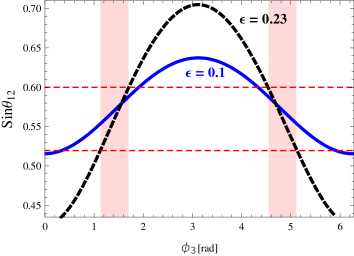
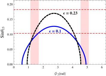
Figure 2: Plots of $\sin\theta_{12}$ and $\sin\theta_{13}$ as a function of $\phi_{3}$ [rad]. The (blue) solid and (black) dashed lines correspond to $\epsilon=0.1$ and $\epsilon=0.23$, respectively, for $\theta=-43^{\circ}$ and $\varphi_{21}=183^{\circ}$. The red bands are allowed regions for $\phi_{3}$ which is constrained by $\sin\theta_{12}$. Here the horizontal dashed lines represent $3\sigma$ experimental bounds in Table 2.

By comparing Eq. (172) with (165) and (166), it is clearly seen that the amount of the modification effects to $\theta_{12}$ and $\theta_{13}$ depends on the parameters $\epsilon$ and $\lambda$. For example, Fig. 2 shows how the solar mixing angle $\theta_{12}$ and reactor mixing angle $\theta_{13}$ depend on the parameters $\phi_{3}$ and $\epsilon$ for fixed values of $\theta$ and $\varphi_{21}$: the (blue) solid and (black) dashed lines correspond to $\epsilon=0.1$ and $\epsilon=0.23$ , respectively, for $\theta=-43^{\circ}$ and $\varphi_{21}=183^{\circ}$ which are chosen to be values a little deviated from $\theta=-45^{\circ}$ and $\varphi_{21}=180^{\circ}$ equivalent to $y_{1,2}=0$. As can be seen in the left plot on $\theta_{12}$ of Fig. 2, for $\epsilon=0.23$, there are two allowed regions on the phase $\phi_{3}$, that is, $1.1\lesssim\phi_{3}{\rm[rad]}\lesssim 1.7$ and $4.6\lesssim\phi_{3}{\rm[rad]}\lesssim 5.1$. The right plot on $\theta_{13}$ of Fig. 2 shows that the measured value of $\theta_{13}$ favors only one region, $1.1\lesssim\phi_{3}{\rm[rad]}\lesssim 1.7$.

Similar to Eq. (167), from Eq. (172) we find a correlation modified by the SM charged lepton sector between the solar mixing angle $\theta_{12}$ and the reactor mixing one $\theta_{13}$:

$$\sin\theta_{12}=\sqrt{\frac{1-2\epsilon\cos\phi_{3}}{3(1-\sin^{2}\theta_{13})}}~{}.$$ (175)

In comparison with Eq. (167), the solar mixing angle in Eq. (175) can be sizably changed by the parameters $\epsilon$ and $\phi_{3}$. Fig. 3 shows a correlation between $\theta_{12}$ and $\theta_{13}$ for $\epsilon=0.23$, where the solid lines correspond to $\phi_{3}=2.5,~{}1.7,~{}1.1,~{}0.4$ [rad] from the bottom, respectively. For a fixed value $\epsilon=0.23$, there is a region of $\phi_{3}$, i.e. $1.1\lesssim\phi_{3}{\rm[rad]}\lesssim 1.7$, satisfying the experimental data of $\theta_{12}$ and $\theta_{13}$ at $3\sigma$. Comparing Fig. 3 to Fig. 1, we see that the value of $\sin\theta_{12}$ can vary to a large extent, depending on $\phi_{3}$ which arises from the SM charged lepton effects.

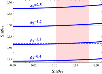
Figure 3: Plot of $\sin\theta_{12}$ versus $\sin\theta_{13}$ with the varying phase $\phi_{3}$ [rad] for $\epsilon=0.23$. Here the horizontal dashed lines and red band represent $3\sigma$ experimental bounds of $\theta_{12}$ and $\theta_{13}$, respectively, in Table 2.

Also, the atmospheric mixing angle can be modified as

$$\sin^{2}\theta_{23} = \frac{|U^{v}_{23}-U^{\ell}_{23}U^{v}_{33}+U^{\ell\ast}_{12}U^{v}_{13}|^{2}}{1-|U^{v}_{13}-U^{\ell}_{12}U^{v}_{23}-U^{\ell}_{13}U^{v}_{33}|^{2}}\simeq\frac{1-\sin 2\theta\cos(2\pi/3-\varphi_{21})-\epsilon\lambda}{2+\sin 2\theta\cos\varphi_{21}-\epsilon\lambda}~{},$$ (176)

where we have used Eq. (174). Again, the amount of the modification effects to $\theta_{12}$ and $\theta_{23}$ depends on the parameters $\epsilon$ and $\lambda$. It is very interesting to note that for $\sin 2\theta\approx-1$ and $\cos\phi_{3}\simeq-1$, we have  $\lambda\approx 0$, in which case the angle $\theta_{23}$ is not much modified from that in Eq. (166), but only $\theta_{12}$ can be modified sizably by the SM charged lepton part. For an illustration, we show plots of $\sin\theta_{12}$ in the left plot of Fig. 2 and $\sin\theta_{23}$ in the left plot of Fig. 4 as a function of $\phi_{3}$[rad], respectively: in both plots, the (blue) solid and (black) dashed lines correspond to $\epsilon=0.1$ and $\epsilon=0.23$, respectively, for $\theta=-43^{\circ}$ and $\varphi_{21}=183^{\circ}$. Here the horizontal dotted lines represent $3\sigma$ experimental bounds in Table 2. And the red bands come from the constraint of experimental data of $\theta_{12}$. We see that the value of $\sin\theta_{12}$ is sensitive to $\phi_{3}$ and $\epsilon$, while the value of $\sin\theta_{23}$ varies relatively small. In particular, from Figs. 2 and 4, one can see the deviations of $\sin\theta_{12}$, $\sin\theta_{23}$ and $\sin\theta_{13}$ from their TBM values of $1/\sqrt{3}$, $1/\sqrt{2}$ and 0, respectively, depending on $\phi_{3}$ and $\epsilon$. It is also obvious from these two figures that there are allowed values of $\phi_{3}$ and $\epsilon$ to satisfy the $3\sigma$ experimental bounds on $\sin\theta_{12}$, $\sin\theta_{23}$ and $\sin\theta_{13}$: e.g., $\phi_{3}\sim 1.5$ [rad] for both $\epsilon=0.1$ and 0.23.

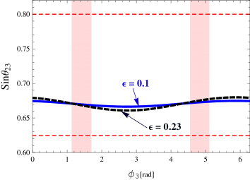
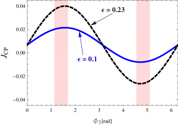
Figure 4: Plots of $\sin\theta_{23}$ (left) and $J_{CP}$ (right) as a function of $\phi_{3}$ [rad]. In both plots, the (blue) solid and (black) dashed lines correspond to $\epsilon=0.1$ and $\epsilon=0.23$, respectively, for $\theta=-43^{\circ}$ and $\varphi_{21}=183^{\circ}$. Here the horizontal dashed lines represent $3\sigma$ experimental bounds of $\theta_{23}$ in Table 2. The red bands come from the constraint of the experimental data $\theta_{12}$.

Interestingly enough, CP violating phases arise from the dimension-five operators driven by the $\chi$ field and they are directly related to the low energy Dirac CP phase which can be measured, in principle, in long baseline neutrino oscillation experiments Freund:1999gy . By using the conventional parametrization of the PMNS matrix pdg and Eq. (171) one can deduce a expression for Dirac CP phase $\delta_{CP}$ which can be written as

$$\delta_{CP} = -\arg\left(\frac{\frac{U^{\ast}_{e1}U_{e3}U_{\tau 1}U^{\ast}_{\tau 3}}{c_{12}c^{2}_{13}c_{23}s_{13}}+c_{12}c_{23}s_{13}}{s_{12}s_{23}}\right)~{}.$$ (177)

Equivalently, the strength of the low energy CP violation measurable through neutrino oscillation defined by Jarlskog invariant, $J_{CP}={\rm Im}[U_{e1}U_{\mu 2}U^{\ast}_{e2}U^{\ast}_{\mu 1}]$, could be expressed roughly in terms of our parameters

$$J_{CP} \simeq \frac{\sqrt{3}}{18}\left(\cos 2\theta+\epsilon\sin 2\theta(\sqrt{3}\cos\varphi_{21}-\sin\varphi_{21})\sin\phi_{3}\right)~{}.$$ (178)

The right plot of Fig. 4 shows the behavior of the $J_{CP}$ as a function of $\phi_{3}$. As pointed out in Fig. 2, the measured value of $\theta_{13}$ favors the region $1.1\lesssim\phi_{3}{\rm[rad]}\lesssim 1.7$, which in turn means that $J_{CP}$ has a non-vanishing value, indicating a signal of maximal $CP$ violation.

It is worth noting that the features discussed above can be similarly obtained also in the Type I seesaw case with the $A_{4}\times Z_{2}$ symmetry. In the Type III seesaw case, because of their origin from the same $SU(2)_{L}$ triplet, the heavy neutral ($N$) and charged ($E$) leptons appear in the Lagrangian usually on the same footing, as shown in the previous and this section. It is thus unlikely in the Type III seesaw with the $A_{4}\times Z_{2}$ symmetry to find sizable effects from only either $N$ or $E$ to the charged lepton mass terms or the neutrino Dirac mass terms. However, the presence of the heavy charged lepton ($E$) in the Type III case leads to unique physical consequences differentiating from those of the Type I case, such as decays of $E$ (through the gauge interactions given in Eq. (90)) and new tree level FCNC processes, which can be tested in future experiments.

IV Conclusion

The seesaw mechanism is a promising way to explain the tiny masses of neutrinos, but it cannot provide a solution for the puzzling pattern of mixing among different lepton flavors. An interesting approach for understanding the pattern of the mixing matrix in the lepton sector is to invoke certain family symmetries which constrain the flavor structure of couplings of Yukawa interactions.

Motivated by the recent neutrino data from Daya Bay and RENO Collaborations, we have studied the phenomenology of neutrino mixing angles in the Type III seesaw model with $A_{4}$ flavor symmetry. Stating with the leptonic Yukawa interactions having a $SU(2)_{L}\times U(1)_{Y}\times A_{4}\times Z_{2}$ symmetry which is spontaneously broken at a scale much higher than the EW scale, we have shown that at tree level the TBM form of the lepton mixing PMNS matrix can be obtained in a natural way. From the current neutrino experimental data, either normal or inverted hierarchical case of neutrino masses is allowed, depending on the sign of a particular parameter in our analysis.

By introducing higher dimensional operators, we have explicitly shown that the lepton mixing matrix generally has a deviation from the TBM form such that it can explain the non-zero mixing angle $\theta_{13}$ indicated by recent experimental data. With negligible corrections from the charged lepton sector to the lepton mixing matrix, our result is consistent with all the neutrino experimental bounds, such as $\Delta m_{\rm sol}^{2}$, $\Delta m_{\rm atm}^{2}$, $\sin^{2}\theta_{12}$, $\sin^{2}\theta_{23}$ and $|U_{e3}|$ at $3\sigma$ level, but our prediction for the possible value of $\sin^{2}\theta_{12}$ is disfavored by the data at $1\sigma$ level. In the presence of effective dimension-5 operators driven by $SU(2)_{L}\times U(1)_{Y}$ singlet scalar fields we have found that sizable contributions from the charged lepton part modify the lepton mixing matrix with which all the neutrino data can be accommodated through phase effects. We have shown that although two regions on the phase $\phi_{3}$, $1.1\lesssim\phi_{3}{\rm[rad]}\lesssim 1.7$ and $4.6\lesssim\phi_{3}{\rm[rad]}\lesssim 5.1$, are allowed by the experimental data of $\theta_{12}$, the measured value of $\theta_{13}$ favors the former. In particular, the recently measured best-fit value of $\theta_{13}=8.68^{\circ}$ can be understood in our framework in a consistent way with the constraints from the other mixing angles $\theta_{12}$ and $\theta_{23}$. Furthermore, we have found that the leptonic $CP$ violation characterized by the Jarlskog invariant has a non-vanishing value, indicating a signal of maximal $CP$ violation $J_{CP}\simeq 0.04$, which could be tested in the future experiments such as the upcoming long baseline neutrino oscillation ones.

Appendix A

A.1 Comments on Eq. (29)

The term ${\rm Tr}[(\overline{\tilde{\Sigma}^{c}}\Sigma)_{{\bf 3}_{a}}]$ would lead to the terms $[\overline{(N_{R})^{c}}~{}N_{R}]_{{\bf 3}_{a}}$ and $[\overline{(E_{R}^{+})^{c}}~{}E_{R}^{-}]_{{\bf 3}_{a}}$ $+[\overline{(E_{R}^{-})^{c}}~{}E_{R}^{+}]_{{\bf 3}_{a}}$. But, the right-handed Majorana neutrino term $[\overline{(N_{R})^{c}}~{}N_{R}]_{{\bf 3}_{a}}$ identically vanishes due to the property of a Majorana particle. In contrast, for the heavy charged leptons, after $A_{4}$ symmetry breaking, the ${\bf 3_{a}}$ term leads to $\overline{(E_{R}^{+})^{c}}~{}M_{E}^{a}~{}E_{R}^{-}+~{}\overline{(E_{R}^{-})^{c}}~{}M_{E}^{a}~{}E_{R}^{+}=\overline{(E_{R}^{+})^{c}}~{}(M_{E}^{a}+M_{E}^{aT})~{}E_{R}^{-}=0$, where

$$M_{E}^{a}={\left(\begin{array}[]{ccc}0&\lambda^{a}_{\chi}\upsilon_{\chi_{3}}&\lambda^{a}_{\chi}\upsilon_{\chi_{2}}\\ -\lambda^{a}_{\chi}\upsilon_{\chi_{3}}&0&\lambda^{a}_{\chi}\upsilon_{\chi_{1}}\\ -\lambda^{a}_{\chi}\upsilon_{\chi_{2}}&-\lambda^{a}_{\chi}\upsilon_{\chi_{1}}&0\end{array}\right)}=-M_{E}^{aT}~{}.$$ (182)

A.2 Comments on Eq. (83)

The hermitian matrices  $\tilde{m}_{\ell}~{}\tilde{m}^{{\dagger}}_{\ell}$ ,  $\tilde{m}^{{\dagger}}_{\ell}~{}\tilde{m}_{\ell}$ ,  $\tilde{M}_{E}~{}\tilde{M}^{{\dagger}}_{E}$  and  $\tilde{M}^{{\dagger}}_{E}~{}\tilde{M}_{E}$,  respectively, which are given by Bandyopadhyay:2009xa

$$\tilde{m}_{\ell}~{}\tilde{m}^{{\dagger}}_{\ell} = \hat{m}_{\ell}~{}\hat{m}^{{\dagger}}_{\ell}-\Big{(}m^{\prime}_{D}~{}\hat{M}^{-1}~{}\hat{M}^{-1\ast}~{}m^{\prime~{}{\dagger}}_{D}~{}\hat{m}_{\ell}~{}\hat{m}^{{\dagger}}_{\ell}+{\rm H.c.}\Big{)}~{},$$

$$\tilde{m}^{{\dagger}}_{\ell}~{}\tilde{m}_{\ell} = \hat{m}^{{\dagger}}_{\ell}~{}\hat{m}_{\ell}-4~{}\hat{m}^{{\dagger}}_{\ell}~{}m^{\prime}_{D}~{}\hat{M}^{-1}~{}\hat{M}^{-1{\dagger}}~{}m^{\prime~{}{\dagger}}_{D}~{}\hat{m}_{\ell}~{},$$

$$\tilde{M}_{E}\tilde{M}^{{\dagger}}_{E} = \hat{M}~{}\hat{M}^{{\dagger}}+\Big{(}\hat{M}~{}m^{\prime~{}{\dagger}}_{D}~{}m^{\prime}_{D}~{}\hat{M}^{-1}+{\rm H.c.}\Big{)}+2\hat{M}^{-1{\dagger}}~{}m^{\prime~{}{\dagger}}_{D}~{}\hat{m}_{\ell}~{}\hat{m}^{{\dagger}}_{\ell}~{}m^{\prime}_{D}~{}\hat{M}^{-1}$$

$$+\hat{M}^{-1{\dagger}}~{}m^{\prime~{}{\dagger}}_{D}~{}m^{\prime}_{D}~{}m^{\prime~{}{\dagger}}_{D}~{}m^{\prime}_{D}~{}\hat{M}^{-1}+...$$

$$\tilde{M}^{{\dagger}}_{E}\tilde{M}_{E} = ~{}\hat{M}^{{\dagger}}~{}\hat{M}+2m^{\prime~{}{\dagger}}_{D}~{}m^{\prime}_{D}+\Big{(}2~{}\hat{M}^{-1}~{}\hat{M}^{-1{\dagger}}~{}m^{\prime~{}{\dagger}}_{D}~{}\hat{m}_{\ell}~{}\hat{m}^{{\dagger}}_{\ell}~{}m^{\prime}_{D}+{\rm H.c.}\Big{)}+...$$ (183)

Appendix B Higgs Potential and vacuum alignments discussed in Section II

We are going to briefly discuss these vacuum alignments discussed in Sec. II, because it is nontrivial to ensure that the different vacuum alignments of $\langle\varphi^{0}\rangle=(\upsilon,\upsilon,\upsilon)$, $\langle\eta^{0}\rangle=v_{\eta}~{}(\sim v)$ and $\langle\chi\rangle=(\upsilon_{\chi},0,0)$ in Eq. (30) are preserved. There is a generic way to prohibit the problematic interaction terms by physically separating $\chi$ and $(\Phi,\eta)$. Here we solve the vacuum alignment problem by extending the model with a spacial extra dimension $y$ Altarelli:2005yp . We assume that each field lives on the 4D brane either at $y=0$ or at $y=L$, as shown in Fig. 5. The heavy neutrino masses arise from local operators at $y=0$, while the charged fermion masses and the neutrino Yukawa interactions are realized by non-local effects involving both branes. A detailed explanation of this possibility is beyond the scope of this paper.

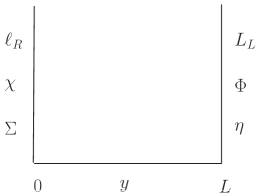
Figure 5: The fifth dimension and locations of scalar and fermion fields.

Then, the most general renormalizable scalar potentials of $\Phi,\eta$ and $\chi$, invariant under $SU(2)_{L}\times U(1)_{Y}\times A_{4}\times Z_{2}$, are given by

$$V_{y=L} = \mu^{2}_{\Phi}(\Phi^{{\dagger}}\Phi)_{\mathbf{1}}+\lambda^{\Phi}_{1}(\Phi^{{\dagger}}\Phi)_{\mathbf{1}}(\Phi^{{\dagger}}\Phi)_{\mathbf{1}}+\lambda^{\Phi}_{2}(\Phi^{{\dagger}}\Phi)_{\mathbf{1^{\prime}}}(\Phi^{{\dagger}}\Phi)_{\mathbf{1^{\prime\prime}}}+\lambda^{\Phi}_{3}(\Phi^{{\dagger}}\Phi)_{\mathbf{3}_{s}}(\Phi^{{\dagger}}\Phi)_{\mathbf{3}_{s}}$$ (184)

$$+ \lambda^{\Phi}_{4}(\Phi^{{\dagger}}\Phi)_{\mathbf{3}_{a}}(\Phi^{{\dagger}}\Phi)_{\mathbf{3}_{a}}+i\lambda^{\Phi}_{5}(\Phi^{{\dagger}}\Phi)_{\mathbf{3}_{s}}(\Phi^{{\dagger}}\Phi)_{\mathbf{3}_{a}}+\mu^{2}_{\eta}(\eta^{{\dagger}}\eta)+\lambda^{\eta}(\eta^{{\dagger}}\eta)^{2}$$

$$+ \lambda^{\Phi\eta}_{1}(\Phi^{{\dagger}}\Phi)_{\mathbf{1}}(\eta^{{\dagger}}\eta)+\lambda^{\Phi\eta}_{2}(\Phi^{{\dagger}}\eta)(\eta^{{\dagger}}\Phi)+\lambda^{\Phi\eta}_{3}(\Phi^{{\dagger}}\eta)(\Phi^{{\dagger}}\eta)+\lambda^{\Phi\eta\ast}_{3}(\eta^{{\dagger}}\Phi)(\eta^{{\dagger}}\Phi)~{},$$

$$V_{y=0} = \mu^{2}_{\chi}(\chi\chi)_{\mathbf{1}}+\lambda^{\chi}_{1}(\chi\chi)_{\mathbf{1}}(\chi\chi)_{\mathbf{1}}+\lambda^{\chi}_{2}(\chi\chi)_{\mathbf{1}^{\prime}}(\chi\chi)_{\mathbf{1}^{\prime\prime}}+\lambda^{\chi}_{3}(\chi\chi)_{\mathbf{3}}(\chi\chi)_{\mathbf{3}}+\xi^{\chi}(\chi\chi\chi)_{\mathbf{1}}~{},$$ (185)

where $\mu_{\Phi},\mu_{\eta},\mu_{\chi}$ and $\xi^{\chi}$ are of the mass dimension 1, while $\lambda^{\Phi}_{1,...,5}$, $\lambda^{\eta}$, $\lambda^{\chi}_{1,...,3}$ and $\lambda^{\Phi\eta}_{1,...,3}$ are all dimensionless. From Eqs. (184) and (185), it is easy to check that the vacuum stabilities of global minima are guaranteed.

The minimum condition of the potential $V_{y=0}$ is

$$\left.\frac{\partial V_{y=0}}{\partial\chi_{1}}\right|_{\langle\chi_{1}\rangle=v_{\chi}}=2v_{\chi}\Big{[}\mu^{2}_{\chi}+2(\lambda_{1}^{\chi}+\lambda_{2}^{\chi})v^{2}_{\chi}\Big{]}=0~{},$$ (186)

and $\left.\frac{\partial V_{y=0}}{\partial\chi_{2,3}}\right|_{\langle\chi_{2,3}\rangle=0}=0$ are automatically satisfied. On the other hand, the minimum conditions for the potential on the brane $y=L$ are

$$\left.\frac{\partial V_{y=L}}{\partial\varphi^{0}_{i}}\right|_{\langle\varphi^{0}_{i}\rangle,\langle\eta\rangle} = 2v\Big{[}\mu^{2}_{\Phi}+2(3\lambda_{1}^{\Phi}+2\lambda_{3}^{\Phi})v^{2}+(\lambda^{\Phi\eta}_{1}+\lambda^{\Phi\eta}_{2}+\lambda^{\Phi\eta}_{3}+\lambda^{\Phi\eta\ast}_{3})v^{2}_{\eta}\Big{]}=0~{},$$

$$\left.\frac{\partial V_{y=L}}{\partial\eta}\right|_{\langle\varphi^{0}_{i}\rangle,\langle\eta\rangle} = 2v_{\eta}\Big{[}\mu^{2}_{\eta}+2\lambda^{\eta}v^{2}_{\eta}+(\lambda^{\Phi\eta}_{1}+\lambda^{\Phi\eta}_{2}+\lambda^{\Phi\eta}_{3}+\lambda^{\Phi\eta\ast}_{3})v^{2}\Big{]}=0~{},$$ (187)

where $\langle\varphi^{0}_{i}\rangle=v~{}(i=1,2,3)$ and $\langle\eta\rangle=v_{\eta}$ are used. We obtain three independent equations for the three unknowns $v$, $v_{\eta}$ and $v_{\chi}$. Thus the configurations needed in our scenario can be realized at tree level. The stability of these vacuum alignments under higher order corrections is not explored in this work.

References

(1)
T. Schwetz, M. Tortola and J. W. F. Valle,
New J. Phys. 13, 109401 (2011)
[arXiv:1108.1376 [hep-ph]];
see also M. C. Gonzalez-Garcia, M. Maltoni and J. Salvado,
JHEP 1004, 056 (2010)
[arXiv:1001.4524v3 [hep-ph]]
;
G. L. Fogli, E. Lisi, A. Marrone, A. Palazzo and A. M. Rotunno,
arXiv:1106.6028 [hep-ph].
(2)
F. P. An et al. [DAYA-BAY Collaboration], [arXiv:1203.1669 [hep-ex]];
J. K. Ahn et al. [RENO Collaboration],
arXiv:1204.0626 [hep-ex]; K. Abe et al. [T2K Collaboration],
Phys. Rev. Lett. 107, 041801 (2011) [arXiv:1106.2822 [hep-ex]];
P. Adamson et al. [MINOS Collaboration],
Phys. Rev. Lett. 107, 181802 (2011) [arXiv:1108.0015 [hep-ex]];
H. De Kerret et al. [Double Chooz Collaboration], talk presented at the Sixth International Workshop on Low Energy Neutrino Physics, November 9-11, 2011 (Seoul, Korea).
(3)
P. A. N. Machado, H. Minakata, H. Nunokawa and R. Z. Funchal,
arXiv:1111.3330 [hep-ph].
(4)
P. F. Harrison, D. H. Perkins and W. G. Scott,
Phys. Lett. B 530, 167 (2002)
[arXiv:hep-ph/0202074].
(5)
Y. Fukuda et al. [Super-Kamiokande Collaboration],
Phys. Rev. Lett. 81, 1562 (1998)
[arXiv:hep-ex/9807003].
(6)
T. Fukuyama and H. Nishiura,
arXiv:hep-ph/9702253;
R. N. Mohapatra and S. Nussinov,
Phys. Rev. D 60, 013002 (1999)
[arXiv:hep-ph/9809415];
E. Ma and M. Raidal,
Phys. Rev. Lett. 87, 011802 (2001)
[Erratum-ibid. 87, 159901 (2001)]
[arXiv:hep-ph/0102255];
C. S. Lam,
Phys. Lett. B 507, 214 (2001)
[arXiv:hep-ph/0104116];
T. Kitabayashi and M. Yasue,
Phys. Rev. D 67, 015006 (2003)
[arXiv:hep-ph/0209294];
A. Ghosal,
arXiv:hep-ph/0304090;
W. Grimus and L. Lavoura,
Phys. Lett. B 572, 189 (2003)
[arXiv:hep-ph/0305046];
J. Phys. G 30, 73 (2004)
[arXiv:hep-ph/0309050];
Y. Koide,
Phys. Rev. D 69, 093001 (2004)
[arXiv:hep-ph/0312207];
Y. H. Ahn, S. K. Kang, C. S. Kim and J. Lee,
Phys. Rev. D 73, 093005 (2006)
[arXiv:hep-ph/0602160];
ibid. D 75, 013012 (2007)
[arXiv:hep-ph/0610007].
(7)
E. Ma and G. Rajasekaran, Phys. Rev. D 64, 113012 (2001) [arXiv:hep-ph/0106291].
(8)
X. G. He, Y. Y. Keum and R. R. Volkas, JHEP 0604, 039 (2006) [arXiv:hep-ph/0601001].
(9)
G. Altarelli, F. Feruglio and C. Hagedorn,
JHEP 0803, 052 (2008)
[arXiv:0802.0090 [hep-ph]];
I. K. Cooper, S. F. King and C. Luhn,
Phys. Lett. B 690, 396 (2010)
[arXiv:1004.3243 [hep-ph]].
(10)
F. Bazzocchi, S. Kaneko and S. Morisi,
JHEP 0803, 063 (2008)
[arXiv:0707.3032 [hep-ph]].
(11)
G. Altarelli and F. Feruglio,
Nucl. Phys. B 720, 64 (2005)
[arXiv:hep-ph/0504165].
(12)
G. Altarelli, F. Feruglio and Y. Lin,
Nucl. Phys. B 775, 31 (2007)
[arXiv:hep-ph/0610165].
(13)
P. Minkowski,
Phys. Lett. B 67, 421 (1977);
T. Yanagida,
in Workshop on Unified Theories, KEK report 79-18 p.95 (1979);
M. Gell-Mann, P. Ramond and R. Slansky,
in Supergravity (North Holland, Amsterdam, 1979)
eds. P. van Nieuwenhuizen, D. Freedman, p.315;
S. L. Glashow,
NATO Adv. Study Inst. Ser. B Phys. 59, 687 (1980);
R. Barbieri, D. V. Nanopoulos, G. Morchio and F. Strocchi,
Phys. Lett. B 90, 91 (1980);
R. N. Mohapatra and G. Senjanovic,
Phys. Rev. Lett. 44, 912 (1980);
G. Lazarides, Q. Shafi and C. Wetterich,
Nucl. Phys. B 181, 287 (1981).
(14)
W. Konetschny and W. Kummer,
Phys. Lett. B 70, 433 (1977);
T. P. Cheng and L. F. Li,
Phys. Rev. D 22, 2860 (1980);
J. Schechter and J. W. F. Valle,
Phys. Rev. D 22, 2227 (1980);
G. Lazarides, Q. Shafi and C. Wetterich,
Nucl. Phys. B 181, 287 (1981);
R. N. Mohapatra and G. Senjanovic,
Phys. Rev. D 23, 165 (1981).
(15)
R. Foot, H. Lew, X. G. He and G. C. Joshi,
Z. Phys. C 44, 441 (1989).
(16)
S. Baek and M. C. Oh,
Phys. Lett. B 690, 29 (2010)
[arXiv:0812.2704 [hep-ph]];
Y. H. Ahn and C. S. Chen,
Phys. Rev. D 81, 105013 (2010)
[arXiv:1001.2869 [hep-ph]];
Y. H. Ahn,
arXiv:1006.2953 [hep-ph];
T. Fukuyama, H. Sugiyama and K. Tsumura,
Phys. Rev. D 82, 036004 (2010)
[arXiv:1005.5338 [hep-ph]].
(17)
E. Ma,
Mod. Phys. Lett. A 17, 535 (2002)
[arXiv:hep-ph/0112232];
Phys. Rev. D 66, 037301 (2002)
[arXiv:hep-ph/0204013];
E. Ma and D. P. Roy,
Nucl. Phys. B 644, 290 (2002)
[arXiv:hep-ph/0206150];
S. M. Barr and I. Dorsner,
Phys. Rev. D 72, 015011 (2005)
[arXiv:hep-ph/0503186];
B. Bajc and G. Senjanovic,
JHEP 0708, 014 (2007)
[arXiv:hep-ph/0612029];
I. Dorsner and P. Fileviez Perez,
JHEP 0706, 029 (2007)
[arXiv:hep-ph/0612216];
P. Fileviez Perez,
Phys. Lett. B 654, 189 (2007)
[arXiv:hep-ph/0702287];
C. Biggio,
Phys. Lett. B 668, 378 (2008)
[arXiv:0806.2558 [hep-ph]];
W. Chao,
arXiv:0806.0889 [hep-ph];
R. N. Mohapatra, N. Okada and H. B. Yu,
Phys. Rev. D 78, 075011 (2008)
[arXiv:0807.4524 [hep-ph]];
M. Hirsch, S. Morisi and J. W. F. Valle,
arXiv:0810.0121 [hep-ph];
R. Adhikari, J. Erler and E. Ma,
arXiv:0810.5547 [hep-ph];
E. Ma,
arXiv:0810.5574 [hep-ph];
J. Chakrabortty, A. Dighe, S. Goswami and S. Ray,
arXiv:0812.2776 [hep-ph];
Y. Liao, J. Y. Liu and G. Z. Ning,
Phys. Rev. D 79, 073003 (2009)
[arXiv:0902.1434 [hep-ph]].
(18)
T. Hambye, Y. Lin, A. Notari, M. Papucci and A. Strumia,
Nucl. Phys. B 695, 169 (2004)
[arXiv:hep-ph/0312203];
A. Strumia,
Nucl. Phys. B 809, 308 (2009)
[arXiv:0806.1630 [hep-ph]];
D. Aristizabal Sierra, J. F. Kamenik and M. Nemevsek,
JHEP 1010, 036 (2010)
[arXiv:1007.1907 [hep-ph]].
(19)
B. Bajc, M. Nemevsek and G. Senjanovic,
Phys. Rev. D 76, 055011 (2007)
[arXiv:hep-ph/0703080];
R. Franceschini, T. Hambye and A. Strumia,
Phys. Rev. D 78, 033002 (2008)
[arXiv:0805.1613 [hep-ph]];
F. del Aguila and J. A. Aguilar-Saavedra,
arXiv:0809.2096 [hep-ph].
Shao-Long Chen and Xiao-Gang He,
arXiv:0901.1264 [hep-ph];
X. G. He, S. Oh, J. Tandean and C. C. Wen,
Phys. Rev. D 80, 073012 (2009)
[arXiv:0907.1607 [hep-ph]].
(20)
A. Abada, C. Biggio, F. Bonnet, M. B. Gavela and T. Hambye,
JHEP 0712, 061 (2007)
[arXiv:0707.4058 [hep-ph]];
Phys. Rev. D 78, 033007 (2008)
[arXiv:0803.0481 [hep-ph]];
E. Fernandez-Martinez, M. B. Gavela, J. Lopez-Pavon and O. Yasuda,
Phys. Lett. B 649, 427 (2007)
[arXiv:hep-ph/0703098];
X. G. He and S. Oh,
JHEP 0909, 027 (2009)
[arXiv:0902.4082 [hep-ph]].
(21)
K. M. Parattu and A. Wingerter,
arXiv:1012.2842 [hep-ph].
(22)
Y. H. Ahn, H. -Y. Cheng and S. Oh,
Phys. Rev. D 83, 076012 (2011) [arXiv:1102.0879 [hep-ph]];
Y. H. Ahn, H. -Y. Cheng and S. Oh,
arXiv:1105.4460 [hep-ph];
Y. H. Ahn, H. -Y. Cheng and S. Oh,
Phys. Rev. D 84, 113007 (2011) [arXiv:1107.4549 [hep-ph]].
(23)
K. Nakamura et al. (Particle Data Group), J. Phys. G 37, 075021 (2010).
(24)
M. Freund, M. Lindner, S. T. Petcov and A. Romanino, Nucl. Phys. B 578, 27 (2000)
[arXiv:hep-ph/9912457];
M. Lindner, Nucl. Phys. Proc. Suppl. 118, 199 (2003) [arXiv:hep-ph/0210377].
(25)
P. Bandyopadhyay, S. Choubey and M. Mitra,
JHEP 0910, 012 (2009)
[arXiv:0906.5330 [hep-ph]].