Fluid phase separation inside a static periodic field: an effectively
two-dimensional critical phenomenon

Abstract

When a fluid with a bulk liquid-vapor critical point is placed inside a static external field with spatial periodic oscillations in one direction, the bulk critical point splits into two new critical points and a triple point. This phenomenon is called laser-induced condensation [Mol. Phys. 101, 1651 (2003)], and it occurs when the wavelength of the field is sufficiently large. The critical points mark the end of two coexistence regions, namely between (1) a vapor and stacked-fluid phase, and (2) a stacked-fluid and liquid phase. The stacked-fluid or “zebra” phase is characterized by large density oscillations along the field direction. We study the above phenomenon for a mixture of colloids and polymers using density functional theory and computer simulation. The theory predicts that the vapor-zebra and liquid-zebra surface tensions are extremely small. Most strikingly, however, is the theoretical finding that at their respective critical points, both tensions vanish, but not according to any critical power law. The solution to this apparent paradox is provided by the simulations. These show that the field divides the system into effectively two-dimensional slabs, stacked on top of each other along the field direction. Inside each slab, the system behaves as if it were two-dimensional, while in the field direction the system resembles a one-dimensional Ising chain.

I Introduction

Binary mixtures of sterically-stabilized colloids and non-adsorbing globular polymers are valuable model systems. In particular, the addition of polymers causes an effective depletion attraction between the colloids. This can induce liquid-vapor type transitions in these systems, in much the same way as in an atomic fluid. Indeed, liquid-vapor demixing in colloid-polymer mixtures has been routinely studied in the past, using theory, computer simulation, and experiment Brader2003 ; Lekkerkerker1992 ; Poon2002 ; Tuinier2008 ; Bolhuis2002 ; Dzubiella2001 . More phenomena for which colloid-polymer mixtures are ideal model systems include equilibrium clustering Stradner2004 , “attractive” glasses Pham2002 ; Zaccarelli2004 , gelation Laurati2009 , numerous interfacial phenomena Vliegenthart1997 ; Hoog1999 ; Chen2000 ; Chen2001 including capillary waves Aarts2004 ; Vink2005 , and wetting Aarts2003 ; Wijting2003 ; Wijting2003a ; Indekeu2010 .

Presumably the simplest model of a colloid-polymer mixture is the one proposed by Asakura and Oosawa (AO) Asakura1954 ; Asakura1958 ; Vrij1976 . Despite its simplicity, this model captures the essential physics Poon2002 ; Bolhuis2002 , yet remains simple enough to allow for both theoretical investigations (based, for instance, on liquid state and density functional theory Schmidt2000 ; Schmidt2002 ), and computer simulations Vink2004 ; Dijkstra2002 . In agreement with experiments, the AO model features a bulk liquid-vapor critical point Lekkerkerker1992 , a freezing transition Zykova-Timan2010 , and also confinement effects at a single wall Wessels2004 ; Wessels2004a , or between two parallel walls Binder2008 ; DeVirgiliis2008 ; DeVirgiliis2007 ; Vink2006a ; Fortini2006 ; Schmidt2003 can be studied using this model. The AO model has also been used to study wetting Brader2000 ; Evans2001 ; Brader2002 , as well as phase separation in porous media Wessels2003 ; Wessels2005 ; Vink2006 ; Pellicane2008 ; Vink2008 ; Vink2009 . Also of interest is the phase behavior of the AO model inside an external field, such as gravity Schmidt2004 ; Jamie2010 , or a spatially-varying periodic field Gotze2003 .

In Ref. Gotze2003, , a colloid-polymer mixture described by the AO model was subjected to a standing-wave external field, wavelength $\lambda$, propagating in one direction (the $z$-direction in what follows). The field is thus effectively one-dimensional. This can be realized in experiments by placing a colloidal suspension inside a standing laser field Freire1994 . While the influence of such a field on the freezing transition has been extensively studied, and is known to induce laser-induced freezing Chaudhuri2005 ; Franzrahe2009 , relatively little is known regarding its effect on the liquid-vapor transition. Regarding the latter, Ref. Gotze2003, proposes the following scenario: for sufficiently large $\lambda$, the bulk liquid-vapor critical point splits into two critical points and a triple point with an intermediate new phase which is partially condensed in slabs perpendicular to the $z$-direction. We call this phase the “zebra” phase in what follows. The results of Ref. Gotze2003, were obtained by using fundamental measure density functional theory for a colloid-polymer mixture described by the AO model.

In this work, we use the same model and technique to calculate the surface tensions between all three coexisting phases. We find that the vapor-zebra and liquid-zebra surface tensions are extremely small. Moreover, to our surprise, upon approach of the critical points, the latter tensions do not yield the expected critical power law behavior. To clarify the nature of the critical points, we use Monte Carlo simulations and finite-size scaling. The simulations confirm all the trends predicted by the theory, and also explain why the vapor-zebra and liquid-zebra surface tensions do not become critical. The main finding is that the standing-wave external field divides the system into effectively two-dimensional slabs, stacked on top of each other along the $z$-direction. Inside each slab, the system behaves as if it were two-dimensional, while in the $z$-direction the system resembles an effectively one-dimensional system. Hence, by turning on the external field, the bulk system is “split-up” into $2+1$ separate dimensions. With this picture in mind, most of our observations can be intuitively understood.

II Model and unit conventions

To describe the interactions between colloids (c) and polymers (p) we use the Asakura-Oosawa (AO) model Asakura1954 ; Asakura1958 ; Vrij1976 . The colloids and the polymer coils are both assumed to be spherical objects with respective diameters $\sigma$ and $\sigma_{\rm p}$. In what follows, the colloid diameter $\sigma\equiv 1$ will be the unit of length, and the colloid-to-polymer size ratio is denoted $q=\sigma_{\rm p}/\sigma$. The interaction between colloid-colloid and colloid-polymer pairs is hard-core, while the polymer-polymer interaction is ideal, leading to the following pair potentials

$$u_{\rm cc}(r) = \begin{cases}\infty&r<\sigma\\ 0&\mbox{otherwise,}\end{cases}$$ (1)

$$u_{\rm cp}(r) = \begin{cases}\infty&r<(\sigma+\sigma_{\rm p})/2\\ 0&\mbox{otherwise,}\end{cases}$$ (2)

$$u_{\rm pp}(r) = 0,$$ (3)

with $r$ the center-to-center distance. As the interactions are either hard-core or ideal, the temperature $T$ can be scaled out (it only sets the energy scale $k_{B}T$, where $k_{B}$ is the Boltzmann constant). We mostly use a grand canonical ensemble, i.e. the system volume $V$, the colloid chemical potential $\mu_{\rm c}$, and the polymer chemical potential $\mu_{\rm p}$ are fixed, but the number of colloids ${N_{\rm c}}$ and polymers $N_{\rm p}$ inside $V$ fluctuates. The particle densities are defined as $\rho_{i}=N_{i}/V$, with $i\in(\rm c,p)$. We also introduce the colloid packing fraction $\eta_{\rm c}=\rho_{\rm c}v_{\rm c}$, with $v_{\rm c}=\pi\sigma^{3}/6$ the volume of a single colloid. Following convention Lekkerkerker1992 , we do not use the polymer chemical potential itself, but rather the polymer reservoir packing fraction $\eta_{\rm p}^{\rm r}$. It is defined as the packing fraction $\eta_{\rm p}^{\rm r}\equiv\rho_{\rm p}v_{\rm p}$, $v_{\rm p}=\pi\sigma_{\rm p}^{3}/6$, of a pure polymer system at given $\mu_{\rm p}$ (for the AO model, such a system is simply an ideal gas, and hence $\eta_{\rm p}^{\rm r}\propto e^{\mu_{\rm p}/k_{B}T}$). In order to compare $\mu_{\rm c}$ between theory and simulation, the thermal wavelength $\Lambda=\sigma/2$ in what follows.

In the AO model, there is an effective attraction between the colloids. This can be shown formally by “integrating out” the polymers Asakura1954 ; Dijkstra1999 , which leads to an effective colloid-colloid pair potential with an attractive well; the well-depth is proportional to $\eta_{\rm p}^{\rm r}$. Hence, the bulk AO model undergoes a liquid-vapor type transition, with $\eta_{\rm p}^{\rm r}$ playing the role of inverse temperature (by bulk we explicitly mean a three-dimensional system in the absence of any surfaces or fields).

The extension of this work is to consider the AO model inside an external field propagating along the $z$-direction

$$V_{\rm ext}(z)=V_{0}\cos\left(2\pi z/\lambda\right),$$ (4)

with $V_{0}$ the field amplitude, and $\lambda$ the wavelength. We emphasize that the field is static: it oscillates in space, not in time. Physically, Eq. (4) resembles a one-dimensional standing optical wave, which could easily be realized experimentally using a laser beam. In this work, we assume that Eq. (4) acts on the colloidal particles only, but that the polymers do not “feel” the field. The Hamiltonian of the system is thus defined by the AO pair potentials, Eqs.(1)-(3), plus an external field contribution $\sum_{i=1}^{N_{\rm c}}V_{\rm ext}(z_{i})$, where the sum is over all colloids, and with $z_{i}$ the $z$-coordinate of the $i$-th colloidal particle.

III Density functional theory

In density functional theory (DFT), the equilibrium density profiles are the ones that minimize the grand canonical free energy functional

$$\Omega[T,\mu_{\rm c},\eta_{\rm p}^{\rm r},\rho_{\rm c}(z),\rho_{\rm p}(z)],$$ (5)

where $\rho_{\rm c}(z)$ is the average colloid density at position $z$ along the field direction, and $\rho_{\rm p}(z)$ that of the polymers (we thus use an effectively one-dimensional set-up in our DFT calculations). In what follows, we also use the colloid packing fraction profile $\eta_{\rm c}(z)$, which is simply $\rho_{\rm c}(z)$ multiplied by $v_{\rm c}$. The system is symmetric around $z=0$, and we include periodic boundary conditions. Based on the proof that a free energy functional $\Omega$ indeed exists Mermin1965 , we use the fundamental measure approach of Ref. Schmidt2000, to approximate Eq. (5); see Appendix A for full details. We numerically solve the resulting stationarity equation using a Picard iteration scheme Roth2010 .

III.1 Phase diagram

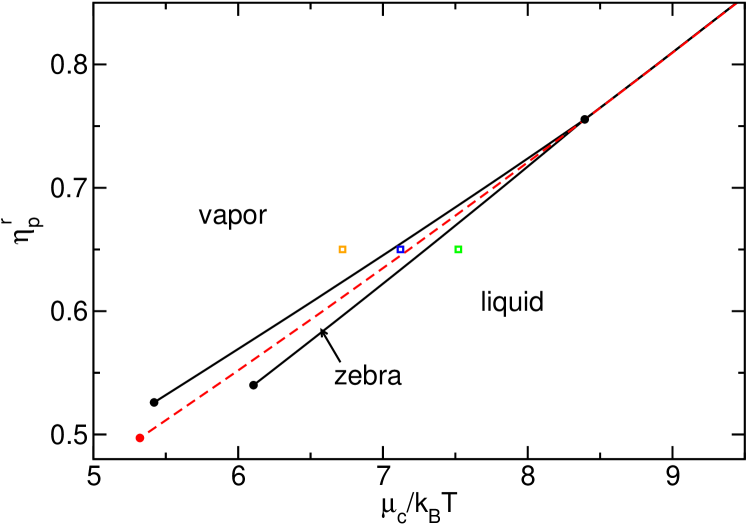
Figure 1: Phase diagram of the AO model with $q=0.6$ in $(\mu_{\rm c},\eta_{\rm p}^{\rm r})$ representation as obtained using DFT. The dashed curve shows the bulk binodal, the solid curves the binodals inside the external field of Eq. (4) using $\lambda=8.192$, and $V_{0}=0.5\,k_{B}T$. The lower three dots indicate critical points, the upper dot the triple point. The open squares denote the state points at which the colloid density profiles of Fig. 3 were measured.

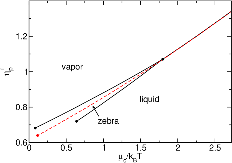
Figure 2: Same as Fig. 1, but using $q=1.0$, with external field parameters $\lambda=10$, and $V_{0}=0.4\,k_{B}T$.

First, we revisit Ref. Gotze2003, and hence choose the size ratio $q=0.6$, the wavelength of the external field $\lambda=8.192$, and its amplitude $V_{0}=0.5\,k_{B}T$. Fig. 1 shows the phase diagram obtained from our DFT calculation. Here, we use the grand canonical representation, i.e. we plot the binodals in the $(\mu_{\rm c},\eta_{\rm p}^{\rm r})$ plane. Clearly visible is the characteristic “inverted letter Y” or “pitchfork” topology (solid lines). For comparison, the dashed line shows the bulk binodal, i.e. obtained without the external potential of Eq. (4). We first note that the bulk critical point occurs at a value of $\eta_{\rm p}^{\rm r}$ below that of the vapor-zebra and liquid-zebra critical points. This is to be expected as confinement generally lowers transition temperatures. The more striking feature of Fig. 1 is that $\eta_{\rm p}^{\rm r}$ of the liquid-zebra critical point exceeds that of the vapor-zebra one: we find $\eta_{\rm p,cr}^{\rm r,vz}\approx 0.526$ and $\eta_{\rm p,cr}^{\rm r,lz}\approx 0.540$. In contrast, in Ref. Gotze2003, , no difference could be detected, which demonstrates the improved accuracy of the present work. The fact that the critical “inverse temperatures” differ is a genuine feature, since our simulations reveal the same trend. As $\eta_{\rm p}^{\rm r}$ increases, the binodals approach each other, and at the triple point, $\eta_{\rm p,tr}^{\rm r}\approx 0.755$, they meet. In order to facilitate the comparison to computer simulation later on, we also present the phase diagram for $q=1$, using field parameters $\lambda=10$, and $V_{0}=0.4\,k_{B}T$ (Fig. 2). We obtain the same overall topology, but the region where the zebra phase occurs has broadened. In addition, the binodals are shifted to significantly lower colloid chemical potential.

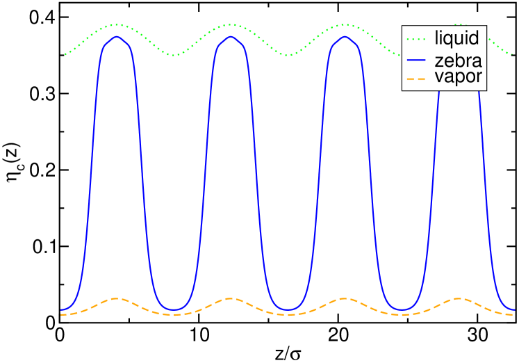
Figure 3: Equilibrium colloid density profiles $\eta_{\rm c}(z)$ measured along the direction of the laser field for the three state points indicated by open squares in the phase diagram of Fig. 1, corresponding to the vapor phase ($\mu_{\rm c}/k_{B}T=6.72$), the zebra phase ($\mu_{\rm c}/k_{B}T=7.12$), and the liquid phase ($\mu_{\rm c}/k_{B}T=7.52$). The profiles were obtained at fixed $\eta_{\rm p}^{\rm r}=0.65$.

Next, we consider the structural properties of the phases. The key difference with the bulk AO model is that, in addition to a vapor and liquid phase, we now also have the zebra phase. The latter phase arises when $\eta_{\rm p}^{\rm r}$ is chosen between the critical and triple points, and with the colloid chemical potential chosen appropriately. To characterize the phases, we have measured colloid density profiles $\eta_{\rm c}(z)$ along the direction of the laser field at three points in the phase diagram of Fig. 1, indicated by open squares. The latter correspond, from left to right, to a vapor state, a zebra state, and a liquid state. The density profiles are shown in Fig. 3. The salient feature is that all three phases display density modulations in the $z$-direction, but the average density and amplitude differ. The average colloid density is low in the vapor phase, high in the liquid phase, with only a modest density amplitude in both phases. The most striking feature of the zebra phase is the unusually large density amplitude, which oscillates between the average density of the vapor and liquid phase.

III.2 Interfaces and interfacial free energies

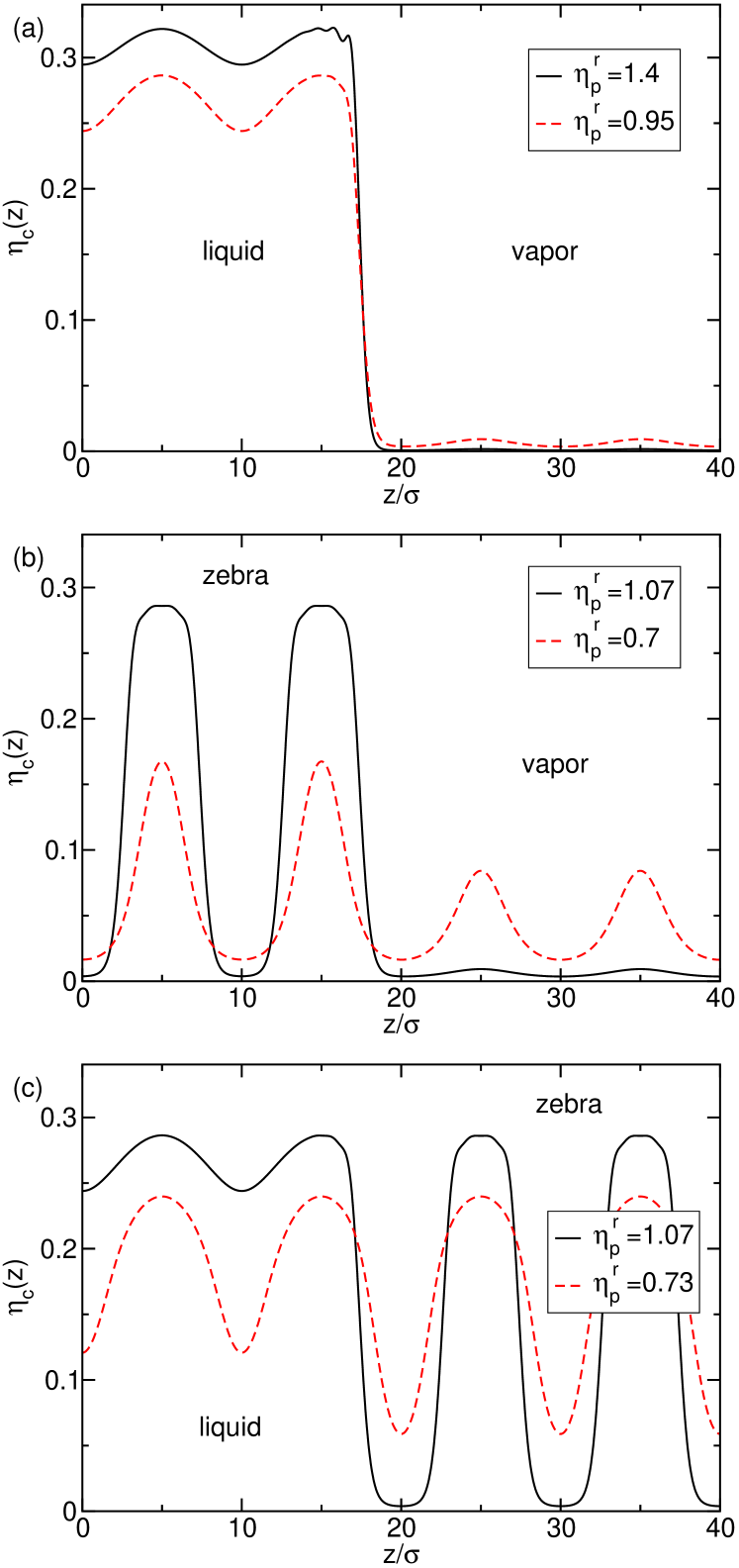
Figure 4: Equilibrium colloid density profiles $\eta_{\rm c}(z)$ showing the various interfaces for the AO model with $q=1$, inside the external field of Eq. (4), using field parameters $\lambda=10$, and $V_{0}=0.4\,k_{B}T$. Shown is the liquid-vapor interface (a), the vapor-zebra interface (b), and the liquid-zebra interface (c), each time for two values of $\eta_{\rm p}^{\rm r}$ as indicated.

We now consider the interfaces between the coexisting phases and the corresponding surface tensions. Above the triple point, $\eta_{\rm p}^{\rm r}>\eta_{\rm p,tr}^{\rm r}$, liquid and vapor coexist, with a corresponding liquid-vapor surface tension $\gamma_{\rm lv}$. To calculate $\gamma_{\rm lv}$, we first compute the equilibrium colloid density profiles $\eta_{\rm c}(z)$ of the pure vapor and liquid phase; the latter yield the Gibbs free energies $\Omega_{\rm v,pure}$ and $\Omega_{\rm l,pure}$, respectively (at coexistence: $\Omega_{\rm v,pure}=\Omega_{\rm l,pure}\equiv\Omega_{\rm pure}$). The density profiles of the pure phases schematically resemble those of Fig. 3. Next, we consider $\eta_{\rm c}(z)$ of a system containing a liquid-vapor interface, from which we obtain $\Omega_{\rm lv,int}$. An example is shown in Fig. 4(a), using two values of $\eta_{\rm p}^{\rm r}$. For sufficiently large $\eta_{\rm p}^{\rm r}$, we observe small oscillations at high densities close to the interface. Since the surface tension is the excess free energy per unit of area, it follows that

$$\gamma_{\rm lv}=\frac{\Omega_{\rm pure}-\Omega_{\rm lv,int}}{2A},$$ (6)

where $A$ is the area of the interface (the factor $1/2$ results from the fact that two interfaces are present in our DFT set-up). The calculation of the vapor-zebra surface tension $\gamma_{\rm vz}$, and of the liquid-zebra surface tension $\gamma_{\rm lz}$, which become defined below the triple point, is performed analogously. To this end, one needs to compute $\eta_{\rm c}(z)$ for a system containing a vapor-zebra and liquid-zebra interface. Some typical density profiles are shown in Fig. 4(b) and (c). It is striking that the interfaces are extremely sharp: even very close to the interface position, the density profiles of the coexisting phases are almost identical to those obtained without the interface! From this observation, and comparing to Eq. (6), one can already deduce that $\gamma_{\rm vz},\gamma_{\rm lz}$ must be very small.

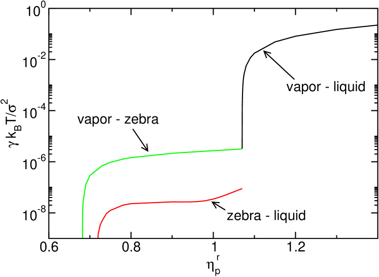
Figure 5: Variation of the surface tensions $\gamma_{\rm lv}$, $\gamma_{\rm vz}$, and $\gamma_{\rm lz}$ with $\eta_{\rm p}^{\rm r}$. Note in particular the extremely small values of $\gamma_{\rm vz}$ and $\gamma_{\rm lz}$. These data were obtained using our DFT for the AO model with $q=1$, and external field parameters $\lambda=10$, $V_{0}=0.4\,k_{B}T$.

In Fig. 5, we summarize the results of the DFT surface tension calculations, where the various tensions are plotted as function of $\eta_{\rm p}^{\rm r}$. Starting above the triple point, $\gamma_{\rm lv}$ is finite; by decreasing $\eta_{\rm p}^{\rm r}$, $\gamma_{\rm lv}$ vanishes at the triple point. At the triple point, $\gamma_{\rm vz}$ and $\gamma_{\rm lz}$ are finite; by decreasing $\eta_{\rm p}^{\rm r}$ further, $\gamma_{\rm vz}$ vanishes at $\eta_{\rm p}^{\rm r}=\eta_{\rm p,cr}^{\rm r,vz}$ of the vapor-zebra critical point, while $\gamma_{\rm lz}$ vanishes at $\eta_{\rm p}^{\rm r}=\eta_{\rm p,cr}^{\rm r,lz}$ of the liquid-zebra critical point. Note the extremely small values of $\gamma_{\rm vz}$ and $\gamma_{\rm lz}$ over the entire range between the critical and triple points. In fact, it always holds that $\gamma_{\rm lv}\geq\gamma_{\rm vz}+\gamma_{\rm lz}$, which implies there is no complete wetting of the “zebra” phase for $\eta_{\rm p}^{\rm r}>\eta_{\rm p,tr}^{\rm r}$.

III.3 Critical behavior

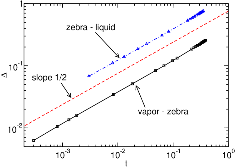
Figure 6: Order parameters $\Delta_{\rm vz}$ and $\Delta_{\rm lz}$ as function of the distance $t$ from their respective critical points, where $\eta_{\rm p,cr}^{\rm r,vz}\approx 0.6817$ and $\eta_{\rm p,cr}^{\rm r,lz}\approx 0.717$ were used. Note the double logarithmic scales! The straight line corresponds to a power law with critical exponent $\beta=1/2$ of mean-field theory. For clarity, the data for $\Delta_{\rm lz}$ have been shifted upward by half a decade.

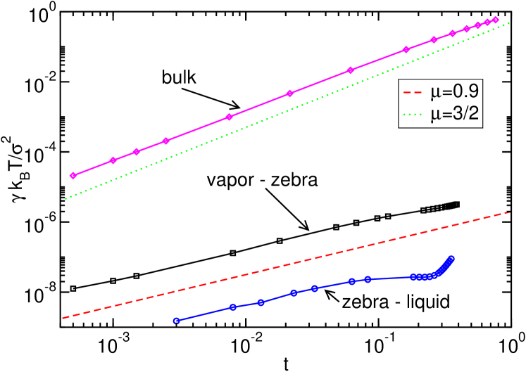
Figure 7: Surface tensions $\gamma_{\rm vz}$, $\gamma_{\rm lz}$, and the bulk liquid-vapor surface tension, as function of the distance $t$ from the respective critical points, where for $\eta_{\rm p,cr}^{\rm r,vz}$ and $\eta_{\rm p,cr}^{\rm r,lz}$ the values of Fig. 6 were used, and $\eta_{\rm p,cr}^{\rm r,bulk}\approx 0.6385$. Note again the double logarithmic scales! The straight line corresponds to a power law with critical exponent $\mu=3/2$ of mean-field theory. The key message is that $\gamma_{\rm vz}$ and $\gamma_{\rm lz}$ do not conform to the mean-field critical exponent (we instead find an exponent $\mu\approx 0.9$).

We now discuss the critical behavior of our equilibrium density profiles close to the vapor-zebra and liquid-zebra critical points. Since our DFT is a mean-field theory, we should recover mean-field critical exponents. This is not to suggest that the universality class of the AO model is the mean-field one – it is not Vink2004 – but rather that we wish to test the internal consistency of our theory. To this end, we introduce the vapor-zebra order parameter

$$\Delta_{\rm vz}=\frac{1}{\lambda}\int_{0}^{\lambda}\eta_{\rm c,z}(z)-\eta_{\rm c,v}(z)\,dz,$$ (7)

where $\eta_{\rm c,z}$ ($\eta_{\rm c,v}$) denotes the equilibrium colloid density profile of the zebra (vapor) phase. Note that $\Delta_{\rm vz}$ above is just the difference between the average colloid density of the vapor and zebra phase. The liquid-zebra order parameter is defined analogously

$$\Delta_{\rm lz}=\frac{1}{\lambda}\int_{0}^{\lambda}\eta_{\rm c,l}(z)-\eta_{\rm c,z}(z)\,dz.$$ (8)

Near the critical points, we expect power law decay of the order parameter

$$\Delta_{\rm x}\propto t^{\beta},\quad t=\eta_{\rm p}^{\rm r}-\eta_{\rm p,cr}^{\rm r,x}>0,\quad\rm x\in(vz,lz),$$ (9)

with critical exponent $\beta=1/2$ for mean-field theory. We compute these order parameters as function of $\eta_{\rm p}^{\rm r}$ and plot them on double logarithmic scales in Fig. 6, where on the horizontal axes the distance from the critical point $t$ is shown. The power law of Eq. (9) with mean-field exponent $\beta=1/2$ is strikingly confirmed!

Next, we consider the critical behavior of the vapor-zebra and liquid-zebra surface tension

$$\gamma_{\rm x}\propto t^{\mu},\quad\rm x\in(vz,lz),$$ (10)

with $t>0$ defined as above, and where the critical exponent $\mu=3/2$ for mean-field theory. In Fig. 7, we plot both surface tensions as function of $t$, again using double logarithmic scales (this plot is simply a rescaling of the data of Fig. 5). For completeness, we also show the liquid-vapor surface tension of the bulk AO model, i.e. in the absence of the laser field. The puzzling result is that, while the bulk tension conforms to $\mu=3/2$ as expected, we do not recover the expected mean-field critical exponent for the vapor-zebra and liquid-zebra surface tensions. From this we conclude that $\gamma_{\rm vz}$ and $\gamma_{\rm lz}$ do not become critical. We postulate there must be a “hidden” surface tension $\gamma_{\rm h}$ which instead conforms to Eq. (10) at the vapor-zebra and liquid-zebra critical points; finding the corresponding “hidden” surface is one of the challenges facing the simulations.

IV Monte Carlo results

We now use computer simulations to corroborate the DFT findings, and to shed light on the peculiar nature of the vapor-zebra and liquid-zebra critical points. We simulate the AO model (defined in Section II) inside the external potential of Eq. (4) using grand canonical Monte Carlo Frenkel2001 . In the grand canonical ensemble, the colloid chemical potential $\mu_{\rm c}$ and the polymer “reservoir packing fraction” $\eta_{\rm p}^{\rm r}$ are fixed, while the number of colloids ${N_{\rm c}}$ and polymers $N_{\rm p}$ in the system fluctuate. We remind the reader that $\eta_{\rm p}^{\rm r}$ plays the role of inverse temperature. To simulate efficiently, a grand canonical cluster move is used Vink2004 , combined with a biased sampling scheme Virnau2004 . The simulations are performed in a $V=L_{x}\times L_{y}\times L_{z}$ box with periodic boundaries. The laser field, Eq. (4), propagates along the edge $L_{z}$ of the box, and hence we choose $L_{z}=n\lambda$, with integer $n>0$, and $\lambda$ the wavelength of the field. In what follows, the colloid-to-polymer size ratio $q=1$, $\lambda=10$, and the laser field amplitude $V_{0}/k_{B}T=0.4$. The key output of the simulations is the order parameter distribution $P(\eta_{\rm c})$ (OPD) defined as the probability to observe the system in a state with colloid packing fraction $\eta_{\rm c}$. From the (normalized) OPD, one readily computes the average colloid packing fraction

$$\langle\eta_{\rm c}\rangle=\int\eta_{\rm c}\,P(\eta_{\rm c})d\eta_{\rm c},$$ (11)

as well as the colloidal compressibility

$$\chi_{\rm c}=V\left(\langle\eta_{\rm c}^{2}\rangle-\langle\eta_{\rm c}\rangle^{2}\right),$$ (12)

and the Binder cumulant Binder1981

$$Q\equiv\langle m^{2}\rangle^{2}/\langle m^{4}\rangle,\quad m=\eta_{\rm c}-\langle\eta_{\rm c}\rangle.$$ (13)

We emphasize that the above quantities, as well as the OPD, depend on all the model parameters, in particular the system size, the imposed colloid chemical potential $\mu_{\rm c}$, and the “inverse temperature” $\eta_{\rm p}^{\rm r}$.

IV.1 Phase diagram

Figure 8: This figure illustrates how the vapor-zebra (VZ) and liquid-zebra (LZ) transitions are located in grand canonical simulations; $\eta_{\rm p}^{\rm r}=1.0$, $L_{x}=L_{y}=12$, and $L_{z}=2\lambda=20$ are used in both plots. (a) The colloidal compressibility $\chi_{\rm c}$ versus the colloid chemical potential $\mu_{\rm c}$; the chemical potential of the left (right) peak yields $\mu_{\rm c}^{\rm vz}$ ($\mu_{\rm c}^{\rm lz}$). (b) The cumulant $Q$ as function of $\langle\eta_{\rm c}\rangle$ (solid curve). The dashed curve shows the compressibility $\chi_{\rm c}$ on an arbitrary vertical scale. The compressibility maxima coincide with maxima in $Q$, the adjacent minima of which are labeled $A,B,C,D$. The horizontal double-arrows mark the vapor-zebra and liquid-zebra order parameters.

Figure 9: Phase diagram of the AO model inside the laser field of Eq. (4) in grand canonical representation (a) and reservoir representation (b); dots mark the critical points obtained via finite-size scaling. No scaling analysis was performed to locate the triple point, but based on the merging of the curves in (a), and also on the shape of the OPD (Fig. 17), we expect that $\eta_{\rm p,tr}^{\rm r}\sim 1.21-1.22$ (horizontal lines). The dashed curves in (b) are power laws corresponding to the critical exponent $\beta$ obtained in Fig. 10(b). As the system size is increased, the binodals obtained in the finite system (solid curves) smoothly approach these power laws. Also labeled in (b) are the various coexistence regions.

To obtain the phase diagram, we vary the colloid chemical potential $\mu_{\rm c}$ at fixed “inverse temperature” $\eta_{\rm p}^{\rm r}$; phase transitions correspond to peaks in the colloidal compressibility. An example is shown in Fig. 8(a), where $\chi_{\rm c}$ versus $\mu_{\rm c}$ is plotted. We observe two sharp peaks, indicating two transitions. The left (right) peak corresponds to the vapor-zebra (liquid-zebra) transition, and from the peak position $\mu_{\rm c}^{\rm vz}$ ($\mu_{\rm c}^{\rm lz}$) can be “read-off”. Note that, above the triple point ($\eta_{\rm p}^{\rm r}>\eta_{\rm p,tr}^{\rm r}$), $\chi_{\rm c}$ versus $\mu_{\rm c}$ reveals only one peak, then corresponding to a liquid-vapor transition. For a range of $\eta_{\rm p}^{\rm r}$, we record the value(s) of the colloid chemical potential where $\chi_{\rm c}$ is maximal, and plot these as points in the $(\mu_{\rm c},\eta_{\rm p}^{\rm r})$ plane. The resulting phase diagram is shown in Fig. 9(a), and the “inverted letter Y” topology predicted by the DFT is strikingly confirmed.

Figure 10: Finite-size scaling analysis of the vapor-zebra critical point. In both plots, $L_{x}=L_{y}=L$ is varied, while $L_{z}=2\lambda$ is fixed. (a) The cumulant $Q_{\rm vz}$ versus $\eta_{\rm p}^{\rm r}$ for different $L$; the intersection yields $\eta_{\rm p,cr}^{\rm r,vz}$. Note that, to the left (right) of the intersection, the cumulants approach $1/3$ ($0$), in agreement with Eq. (16). (b) Scaling plot of the vapor-zebra order parameter. Plotted is $\Delta_{\rm vz}L^{\beta/\nu}$ versus $tL^{1/\nu}$, where $\nu$ and $\beta$ were tuned until a good collapse of the data was observed.

The dots in Fig. 9 mark the vapor-zebra and liquid-zebra critical points, which we obtained using finite size scaling. For a given value of $\eta_{\rm p}^{\rm r}$ and system size, we vary the colloid chemical potential $\mu_{\rm c}$, and record the average colloid packing fraction $\langle\eta_{\rm c}\rangle$, the colloidal compressibility $\chi_{\rm c}$, and the Binder cumulant $Q$. A typical result is shown in Fig. 8(b), where $Q$ and $\chi_{\rm c}$ versus $\langle\eta_{\rm c}\rangle$ are plotted (these curves are thus parametrized by $\mu_{\rm c}$). The key message of Fig. 8(b) is that the compressibility maxima of the vapor-zebra and liquid-zebra transitions coincide with maxima in the cumulant. Adjacent to the cumulant maximum of the vapor-zebra transition, we observe two minima, indicated by the points

$$A\equiv\left(\langle\eta_{\rm c}\rangle_{\rm vz}^{-},\,Q^{-}_{\rm vz}\right),\quad B\equiv\left(\langle\eta_{\rm c}\rangle_{\rm vz}^{+},\,Q^{+}_{\rm vz}\right),$$ (14)

and, similarly, for the liquid-zebra transition

$$C\equiv\left(\langle\eta_{\rm c}\rangle_{\rm lz}^{-},\,Q^{-}_{\rm lz}\right),\quad D\equiv\left(\langle\eta_{\rm c}\rangle_{\rm lz}^{+},\,Q^{+}_{\rm lz}\right).$$ (15)

In the thermodynamic limit, it holds that Kim2005 ; Kim2003

$$\lim_{L_{x},L_{y},L_{z}\to\infty}Q_{\rm vz}=\begin{cases}1/3&\eta_{\rm p}^{\rm r}<\eta_{\rm p,cr}^{\rm r,vz},\\ 0&\eta_{\rm p}^{\rm r}>\eta_{\rm p,cr}^{\rm r,vz},\end{cases}$$ (16)

with $Q_{\rm vz}\equiv(Q^{-}_{\rm vz}+Q^{+}_{\rm vz})/2$, and $\eta_{\rm p,cr}^{\rm r,vz}$ the value of $\eta_{\rm p}^{\rm r}$ at the vapor-zebra critical point. Hence, by plotting $Q_{\rm vz}$ versus $\eta_{\rm p}^{\rm r}$ for a number of different system sizes, curves for different system sizes intersect at $\eta_{\rm p}^{\rm r}=\eta_{\rm p,cr}^{\rm r,vz}$, which can be used to locate the critical point. Of course, to locate the liquid-zebra critical point, one analogously analyzes $Q_{\rm lz}\equiv(Q^{-}_{\rm lz}+Q^{+}_{\rm lz})/2$.

To perform the finite-size scaling analysis, we vary the lateral box extensions $L_{x}=L_{y}\equiv L$, but keep the elongated extension fixed at $L_{z}=2\lambda=20$. We assume that the divergence of the correlation length is “cut-off” in the $z$-direction by the laser field, and so we do not need to scale in this direction (this assumption will be justified in the next section where the static structure factor is discussed). Since the correlations diverge only in the two lateral directions, the critical behavior is effectively two-dimensional. In Fig. 10(a), we plot $Q_{\rm vz}$ versus $\eta_{\rm p}^{\rm r}$ for three values of $L$. In agreement with Eq. (16), an intersection point is observed, from which we conclude that $\eta_{\rm p,cr}^{\rm r,vz}\approx 0.975$. A similar analysis of the liquid-zebra transition yields $\eta_{\rm p,cr}^{\rm r,lz}\approx 1.043$ (not shown). It is striking that the scaling analysis confirms the DFT prediction $\eta_{\rm p,cr}^{\rm r,lz}>\eta_{\rm p,cr}^{\rm r,vz}$. To estimate the colloid chemical potential $\mu_{\rm c,cr}^{\rm vz}$ of the vapor-zebra critical point in the thermodynamic limit, we measured $\mu_{\rm c}^{\rm vz}$ of the compressibility maximum at $\eta_{\rm p}^{\rm r}=\eta_{\rm p,cr}^{\rm r,vz}$ for finite $L$, and extrapolated to $L\to\infty$ assuming $\mu_{\rm c,cr}^{\rm vz}-\mu_{\rm c}^{\rm vz}\propto 1/L$. In this extrapolation, we ignore all subtleties concerning field and pressure mixing Kim2004 , but emphasize that such effects are tiny on the scale of the phase diagram in Fig. 9(a). The resulting estimate reads as $\mu_{\rm c,cr}^{\rm vz}\approx 1.29$, while for the liquid-zebra transition $\mu_{\rm c,cr}^{\rm lz}\approx 1.75$ is obtained.

Next, we consider the scaling of the order parameter. The cumulant minima $A$ and $B$ of Fig. 8(b) readily yield $\Delta_{\rm vz}=\langle\eta_{\rm c}\rangle_{\rm vz}^{+}-\langle\eta_{\rm c}\rangle_{\rm vz}^{-}$ as order parameter for the vapor-zebra transition. In the vicinity of the critical point $\Delta_{\rm vz}\propto t^{\beta}$, with $t=(\eta_{\rm p}^{\rm r}-\eta_{\rm p,cr}^{\rm r,vz})/\eta_{\rm p,cr}^{\rm r,vz}$, $t>0$, and critical exponent $\beta$. The result is shown in Fig. 10(b), where we used the standard finite-size scaling practice Newman1999 of plotting $\Delta_{\rm vz}L^{\beta/\nu}$ versus $tL^{1/\nu}$, with $\nu$ the correlation length critical exponent. Provided suitable values of $\eta_{\rm p,cr}^{\rm r,vz}$, $\beta$ and $\nu$ are used, the data for different $L$ collapse. Reasonable collapses can indeed be realized, using for $\eta_{\rm p,cr}^{\rm r,vz}$ the cumulant intersection estimate of Fig. 10(a), $\beta/\nu\sim 0.25-0.35$, and $\nu\sim 0.85-1.10$. An analysis of $\Delta_{\rm lz}$, which one obtains from the minima $C$ and $D$ of Fig. 8(b), yields similar results (not shown).

Finally, with the critical point parameters known, it becomes possible to calculate the phase diagram in reservoir representation, as is commonly done for the AO model. To this end, we record the colloid packing fraction of each of the cumulant minima $A,B,C,D$ in Fig. 8(b) as function of $\eta_{\rm p}^{\rm r}$; the latter “trace-out” a curve (binodal) in the $(\eta_{\rm c},\eta_{\rm p}^{\rm r})$ plane. The result is shown in Fig. 9(b), where dots again mark the critical points. To estimate the colloid packing fraction of the vapor-zebra critical point, we measured the finite-size “diameter” $\delta_{L,\rm vz}\equiv(\langle\eta_{\rm c}\rangle_{\rm vz}^{-}+\langle\eta_{\rm c}\rangle_{\rm vz}^{+})/2$, using $\eta_{\rm p}^{\rm r}=\eta_{\rm p,cr}^{\rm r,vz}$ and the colloid chemical potential $\mu_{\rm c}^{\rm vz}$ of the compressibility maximum; the diameter was then extrapolated to $L\to\infty$ assuming $\delta_{\infty,\rm vz}-\delta_{L,\rm vz}\propto 1/L$, which again ignores field and pressure mixing effects Kim2004 . In this way $\delta_{\infty,\rm vz}\approx 0.055$ is obtained, while an analogous procedure for the liquid-zebra critical point yields $\delta_{\infty,\rm lz}\approx 0.203$.

IV.2 Nature of the critical point

Figure 11: The colloid-colloid static structure factors obtained at the vapor-zebra critical point. (a) The structure factor $S_{\parallel}(q)$ measured in the direction of the laser field for several values of $L_{z}$, and fixed $L_{x}=L_{y}=10$. There is no divergence as $q\to 0$, indicating that critical fluctuations in the direction of the field are “cut-off”. (b) The structure factor $S_{\perp,z}(q)$ measured in directions perpendicular to the laser field for several values of $z$; the system size used equals $L_{x}=L_{y}=20$, and $L_{z}=4\lambda$. The key message is that $S_{\perp,z}(q)$ diverges as $q\to 0$, but only for selected values of $z$.

A key assumption in the finite-size scaling analysis of the previous section is that the critical correlations are “cut-off” in the $z$-direction, i.e. the direction along which the laser field of Eq. (4) propagates. To justify this assumption, we consider the colloid-colloid static structure factor $S(\vec{q})=\langle\frac{1}{n_{\rm c}}|\sum_{j=1}^{n_{\rm c}}\exp(i\vec{q}\cdot\vec{r}_{j})|^{2}\rangle$, with $\langle\cdot\rangle$ a thermal average, the sum over all $j=1,\ldots,n_{\rm c}$ colloidal particles whose centers are inside a test volume $v$, and $\vec{r}_{j}$ the position of the $j$-th colloid. As usual, wavevectors are given by $\vec{q}=2\pi(k/L_{x},l/L_{y},m/L_{z})$, integers $k,l,m\geq 0$, with the constraint that $k+l+m\neq 0$. We also introduce the wavevector magnitude $q^{2}=\vec{q}\cdot\vec{q}$.

To probe the correlations in the $z$-direction, we use as test volume $v$ a narrow cylinder, with a diameter equal to the colloid diameter, placed parallel to the $z$-axis; due to the symmetry of the system, the location where the cylinder intersects the $xy$-plane is irrelevant. We then calculate the structure factor $S_{\parallel}(q)$, which is obtained using only the wavevectors $\vec{q}_{\parallel}\equiv 2\pi(0,0,m/L_{z})$. In Fig. 11(a), we plot $S_{\parallel}(q)$ measured at the vapor-zebra critical point. These data were obtained in a semi-grand canonical ensemble: the colloid packing fraction and $\eta_{\rm p}^{\rm r}$ are fixed to their critical values ($\eta_{\rm c}=\delta_{\infty,\rm vz},\,\eta_{\rm p}^{\rm r}=\eta_{\rm p,cr}^{\rm r,vz}$), while the number of polymers fluctuates. The important message to take from Fig. 11(a) is that, in the limit $q\to 0$, there is no sign of a divergence $S_{\parallel}(q)\to\infty$. Hence, there are no critical fluctuations in the $z$-direction. Note that the peak at $q\approx 0.63$ corresponds precisely to $2\pi/\lambda$ of the laser field. The analysis of $S_{\parallel}(q)$ at the liquid-zebra critical point leads to similar conclusions (not shown).

Next, we consider the static structure factor $S_{\perp,z}(q)$ measured in the lateral $xy$-directions, i.e. perpendicular to the laser field. In this case, wavevectors take the form $\vec{q}_{\perp}\equiv 2\pi(k/L_{x},l/L_{y},0)$, and as test volume $v$ we use a narrow $L_{x}\times L_{y}\times\Delta z$ slab, placed parallel to the $xy$-plane at “height” $z$ (the slab thickness $\Delta z$ equals one colloid diameter). Since the system is not translation invariant in the $z$-direction, it matters at which $z$-coordinate the slab is located, and so $S_{\perp,z}(q)$ depends on $z$. In Fig. 11(b), we plot $S_{\perp,z}(q)$ at the vapor-zebra critical point for several $z$, again obtained using the semi-grand canonical ensemble. The key message to take from Fig. 11(b) is that $S_{\perp,z}(q)$ does diverge as $q\to 0$, but only for certain values of $z$. The analysis of $S_{\perp,z}(q)$ at the liquid-zebra critical point leads to similar conclusions (not shown).

Figure 12: Profiled quantities obtained at the vapor-zebra critical point. (a) The variation of $S_{\perp,z}(q_{\rm min})$ with $z$ for several $L$. (b) The average colloid packing fraction $\eta_{\rm c}(z)$ measured along the $z$-direction (solid curve). The dashed curve shows the external laser potential of Eq. (4) on an arbitrary vertical scale; regions dense in colloids coincide with minima of the potential.

Figure 13: The analogue of Fig. 12 for the liquid-zebra critical point. In (a), $\gamma/\nu=1.4$ is used.

To summarize: From the static structure factor $S_{\parallel}(q)$, we conclude that critical fluctuations in the $z$-direction are absent. This justifies our previous assumption that the critical behavior is effectively two-dimensional, such that finite-size scaling may be performed by varying only the lateral box extensions $L_{x}=L_{y}=L$, while keeping $L_{z}$ fixed. The analysis of $S_{\perp,z}(q)$ reveals that critical fluctuations indeed develop in the lateral directions, but only at certain $z$ values. The critical behavior is thus localized in effectively two-dimensional slabs perpendicular to the laser field, “sandwiched” between slabs where the system is non-critical. To make this explicit, we show in Fig. 12(a) the variation of $S_{\perp,z}(q_{\rm min})$ with $z$ for the vapor-zebra critical point, where $q_{\rm min}=2\pi/L$ denotes the magnitude of the smallest accessible lateral wavevector. The figure strikingly shows that $S_{\perp,z}(q_{\rm min})$ diverges with $L$ only at selected $z$ values, i.e. the critical behavior is indeed spatially localized in slabs. Note that the critical slabs correspond to regions of enhanced colloid density: $S_{\perp,z}(q_{\rm min})$ is “in-phase” with the colloid density profile $\eta_{\rm c}(z)$ (Fig. 12(b)). Interestingly, at the liquid-zebra critical point, this trend is reversed (Fig. 13). Since $S_{\perp,z}(q_{\rm min})\propto\chi_{\rm c}$ Rowlinson1982 , with $\chi_{\rm c}$ the colloidal compressibility, we expect $S_{\perp,z}(q_{\rm min})\propto L^{\gamma/\nu}$ in the critical slabs Newman1999 . Here, $\gamma$ is the compressibility critical exponent; by fitting the peak values in Fig. 12(a) to this scaling law, $\gamma/\nu\sim 1.3-1.4$ is obtained. For the liquid-zebra critical point, a similar ratio is found, see Fig. 13(a), where $S_{\perp,z}(q_{\rm min})L^{-\gamma/\nu}$ versus $z$ is shown (in this scaled representation, the peak values for different $L$ collapse). It is reassuring that the critical exponent ratios obtained in our scaling analysis conform to hyperscaling, $2\beta/\nu+\gamma/\nu=d=2$, as the reader can verify. Interestingly, our critical exponent ratios are rather different from 2D Ising values ($\beta/\nu=1/8,\gamma/\nu=7/4$), which we would naively have come to expect (only our $\nu$ estimate is somewhat consistent with $\nu=1$ of the 2D Ising model).

IV.3 The coexistence region

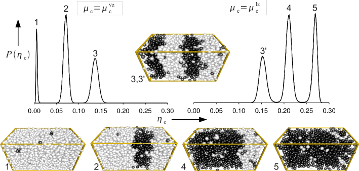
Figure 14: Analysis of the OPD $P(\eta_{\rm c})$ obtained at $\eta_{\rm p}^{\rm r}=1.16$, which is above the critical points, but still below the triple point. The system size used is $L_{z}=2\lambda=20$, and $L_{x}=L_{y}=12$. Shown on the left is $P(\eta_{\rm c})$ at the vapor-zebra transition, while on the right $P(\eta_{\rm c})$ of the liquid-zebra transition is shown. The salient features are a number of peaks, whose meanings become clear upon inspection of snapshots. In the snapshots, the laser field is along the longest edge of the box; colloids are shown as black, polymers as white.

We now consider the vapor-zebra and liquid-zebra two-phase coexistence regions, see Fig. 9(b), where the corresponding transitions are first-order. To this end, we choose $\eta_{\rm p}^{\rm r}$ above the critical points, but still below the triple point, and measure the OPD $P(\eta_{\rm c})$. In Fig. 14, we show $P(\eta_{\rm c})$ using $\mu_{\rm c}=\mu_{\rm c}^{\rm vz}$ of the vapor-zebra transition (left), and using $\mu_{\rm c}=\mu_{\rm c}^{\rm lz}$ of the liquid-zebra transition (right). The striking feature is that the distributions reveal a number of peaks. We first discuss the OPD of the vapor-zebra transition. Here, the left peak (1) reflects the vapor phase, i.e. low colloid density, and high polymer density (see corresponding snapshot 1). Although not visible in the snapshot, we emphasize that the colloid density profile $\eta_{\rm c}(z)$ of the pure vapor phase resembles that of Fig. 3, i.e. there are (small) density modulations along the $z$-direction. The center peak (2) corresponds to a mixed state, where a slab of vapor coexists with a slab of zebra phase (snapshot 2). Hence, a vapor-zebra interface is present, and the corresponding density profile $\eta_{\rm c}(z)$ will schematically resemble Fig. 4(b). Note that, due to periodic boundaries, the number of vapor-zebra interfaces is at least two. The right peak (3) corresponds to a pure zebra phase (snapshot 3), with a density profile resembling the one shown in Fig. 3, i.e. featuring large density oscillations. The meaning of the peaks in the OPD of the liquid-zebra transition follows analogously. In this case, peak 4 reflects liquid-zebra coexistence, to be compared to the profile of Fig. 4(c). Note that the density of the zebra phase at the vapor-zebra transition differs from that of the liquid-zebra transition.

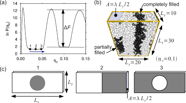
Figure 15: (a) The OPD obtained for $\eta_{\rm p}^{\rm r}=1.16$ at the vapor-zebra transition; shown is $\ln P(\eta_{\rm c})$ versus $\eta_{\rm c}$. The barrier $\Delta F$ reflects the interfacial free energy of the “hidden” interface (see details in text). (b) Snapshot taken at $\eta_{\rm c}=0.1$, which is between the center and right peak of the OPD; the laser field propagates along $L_{z}$. Clearly visible is one completely filled slab, and one partially filled slab. The lateral area $A$ of the “hidden” interface is also indicated, where $\lambda$ is the wavelength of the field (colloids are shown as black, polymers as white). The schematic snapshots in (c) show the partially filled slab along the “path” $1\to 2\to 3$ of (a), where the $z$-direction is perpendicular to the plane of the paper (dark regions correspond to colloid-rich domains).

Also of extreme interest are state points “between the peaks” in the OPD (Fig. 15). Here, we keep $\eta_{\rm p}^{\rm r}=1.16$, but choose larger lateral box extensions, $L_{x}=30$ and $L_{y}=10$, while $L_{z}=2\lambda=20$. In Fig. 15(a), the logarithm of the OPD is shown, using $\mu_{\rm c}=\mu_{\rm c}^{\rm vz}$ of the vapor-zebra transition; note that $\ln P(\eta_{\rm c})$ may be regarded as minus the free energy of the system. As in Fig. 14, three peaks are visible: their meaning is the same as before. The snapshot of Fig. 15(b) was taken at $\eta_{\rm c}=0.1$, which is between the center and right peak of the OPD. Again, vapor-zebra coexistence is observed, but the key difference with the coexistence state points of Fig. 14 is that one of the periods of the field is only partially filled. Hence, in addition to a vapor-zebra interface perpendicular to the field, there is a smaller interface parallel to the field, indicated by the shaded area $A$. This is the “hidden” interface, whose presence was already implied by the DFT calculation. Note that $\ln P(\eta_{\rm c})$ around $\eta_{\rm c}=0.1$ is essentially flat. Hence, once a partially filled slab has formed, it can be filled without any cost in free energy. This can be understood from the schematic snapshots of Fig. 15(c), which show top-down views (i.e. looking along the $z$-direction) of the partially filled slab; the lateral area of the slab equals $L_{x}\times L_{y}$, while the slab thickness equals $\lambda/2$. The snapshots $1,2,3$ in (c) correspond to state points at the minimum between two peaks in the OPD, but with $\eta_{\rm c}$ increasing from left to right (schematically resembling the “path” $1\to 2\to 3$ in Fig. 15(a)). In the first snapshot, a droplet of colloidal liquid has condensed. The droplet is cylindrical in shape; note that the area of the “hidden” interface in this configuration equals the circumference of the circle times the slab thickness. In the second snapshot, the droplet has grown so large it interacts with itself through the periodic boundaries, yielding two slab domains with two interfaces (the snapshot of Fig. 15(b) resembles this situation). Since $L_{x}\gg L_{y}$, the “hidden” interfaces form perpendicular to $L_{x}$; the shaded region $A$ marks the area of one of them. Since the free energy around the minimum of the OPD is flat, it follows that the interfaces do not interact Grossmann1993 , and so we obtain for the surface tension of the “hidden” interface Binder1981

$$\gamma_{\rm h}=\Delta F/2A,$$ (17)

with $A=\lambda L_{y}/2$ (the factor $1/2$ in Eq. (17) is a consequence of periodic boundaries, which lead to the formation of two interfaces). For $\eta_{\rm p}^{\rm r}=1.16$, we obtain $\gamma_{\rm h}\approx 0.1\,k_{B}T/\sigma^{2}$, which significantly exceeds the vapor-zebra surface tension. Finally, by increasing $\eta_{\rm c}$ even further, one obtains the third snapshot, featuring a droplet of colloidal vapor. Note that Fig. 15(c) is just the “standard” droplet condensation transition in a two-dimensional system with periodic boundaries Fischer2010 .

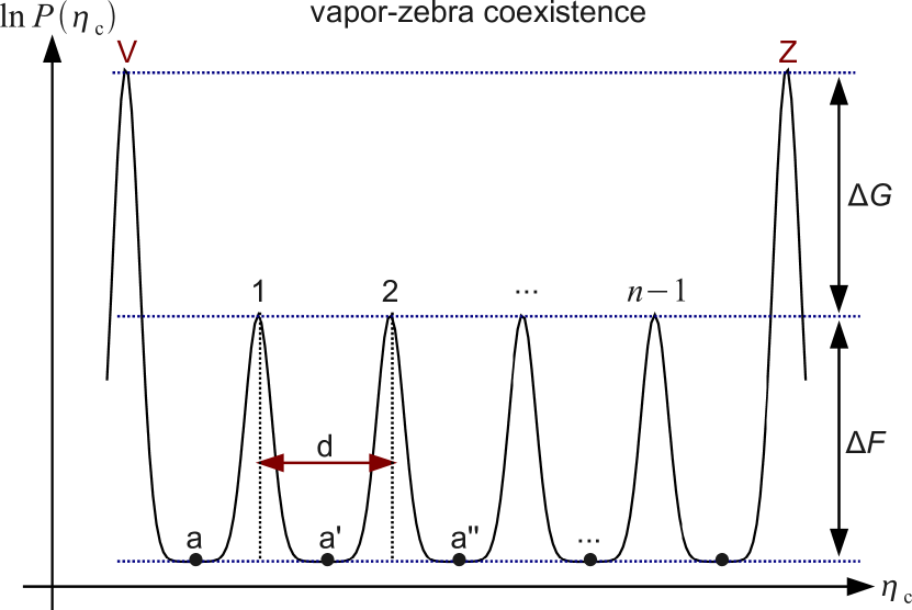
Figure 16: Sketch of the logarithm of the OPD at the vapor-zebra transition, i.e. using $\mu_{\rm c}=\mu_{\rm c}^{\rm vz}$, in a $L\times L\times L_{z}$ periodic box, $L_{z}=n\lambda$, and for $L$ large (solid curve). The two dominating peaks correspond to the pure vapor (V) and zebra phase (Z). The intermediate peaks $1,2,\ldots,n-1$ correspond to states where vapor and zebra coexist, with each period of the field completely filled with either one of the phases. The states $a,a^{\prime},\ldots$ at the minima also correspond to vapor-zebra coexistence, but where one period of the field is only partially filled, as in Fig. 15(b). The barrier $\Delta G$ reflects the free energy cost of the vapor-zebra interface, $\Delta F$ that of the “hidden” interface; the respective scaling is given by Eq. (18).

Having understood the arrangement of the phases in the coexistence region, we expect the OPD at the vapor-zebra transition to scale with system size conform Fig. 16. We assume a $L\times L\times L_{z}$ periodic box, $L_{z}=n\lambda$, with $L$ large. The two dominating peaks correspond to the pure vapor (V) and zebra (Z) phase. The intermediate peaks $1,2,\ldots,n-1$ correspond to states where vapor and zebra coexist, with each period of the field completely filled with either one of the phases. For each additional period of the field, one extra peak arises! The states $a,a^{\prime},\ldots$ at the minima also correspond to vapor-zebra coexistence, but where one period of the field is partially filled, implying the presence of “hidden” interfaces (Fig. 15(b)). In the limit $L_{z}\to\infty$, one thus obtains an infinite sequence of intermediate peaks, separated by “distances” $d\propto 1/L_{z}$. The barrier $\Delta F$ reflects the free energy cost of the “hidden” interface; $\Delta G$ that of the vapor-zebra interface. As $L$ becomes large, we thus expect Binder1981

$$\Delta F=\gamma_{\rm h}\lambda L,\quad\Delta G=2\gamma_{\rm vz}L^{2}.$$ (18)

In the thermodynamic limit $L\to\infty$, $\Delta G$ dominates: the intermediate peaks then become suppressed, and only the pure phase peaks (V,Z) remain. The OPD thus becomes bimodal, as it should since the transition is first-order between two phases Vollmayr1993 . The behavior of the OPD at the liquid-zebra transition follows analogously, although the precise values of $\gamma_{\rm h}$ will differ.

It now becomes clear why $\gamma_{\rm vz}$ and $\gamma_{\rm lz}$ cannot reveal critical behavior. The critical behavior was shown to be effectively two-dimensional, implying that the singular part of the interfacial free energy is due to line tension, i.e. proportional to $L$. As Eq. (18) shows, only the “hidden” interface reveals this required scaling. Consequently, $\gamma_{\rm h}$ becomes critical, while $\gamma_{\rm vz},\gamma_{\rm lz}$ do not.

Figure 17: The OPD $P(\eta_{\rm c})$ at $\eta_{\rm p}^{\rm r}=1.22$ which is close to the triple point; system sizes $L_{x}=L_{y}=8$, $L_{z}=2\lambda=20$ are used. The peaks corresponding to the pure vapor, zebra, and liquid phase are marked (V,Z,L), respectively.

Figure 18: Histogram $H(I)$ of the observed number of vapor-zebra interfaces $I$, obtained during a semi-grand canonical simulation inside the vapor-zebra coexistence region. The key message is that $I$ far exceeds two, showing that the tendency for macroscopic phase separation is weak. This is consistent with the DFT prediction that $\gamma_{\rm vz}$ is extremely small. The dashed curve shows the corresponding histogram for the (exactly known) 1D Ising model at infinite temperature.

Note that the OPDs for finite $L$ do not conform to Fig. 16. For instance, in Fig. 14, the coexistence peaks (2,4) exceed those of the pure phases ($1,3,3^{\prime},5$). This is due to the extremely small values of $\gamma_{\rm vz},\gamma_{\rm lz}$. For the system sizes $L$ accessible in our simulations, $\Delta G$ is essentially zero, meaning that the intermediate peaks are not suppressed. From the finite-size OPD, we thus obtain indirect confirmation of the DFT prediction that $\gamma_{\rm vz},\gamma_{\rm lz}$ are extremely small. A second consequence is that the tendency of the system to macroscopically phase separate is weak. To test this assertion, we performed a semi-grand canonical simulation at $\eta_{\rm c}=0.07$ and $\eta_{\rm p}^{\rm r}=1.16$, using an extremely elongated box with $L_{x}=L_{y}=5$, $L_{z}=50\lambda$. The reader can verify in Fig. 9(b) that this state point is deep inside the vapor-zebra coexistence region. Consequently, we expect macroscopic phase separation, implying the formation of $I=2$ vapor-zebra interfaces (since the system is periodic). In Fig. 18, we have collected a histogram of observed $I$ values, obtained in a long simulation run. The key message is that the number of interfaces far exceeds two, providing further confirmation that $\gamma_{\rm vz}$ is small. In some sense, a $L\times L\times(L_{z}=n\lambda)$ system resembles a set of $i=1,\ldots,n$ slabs; to each slab we may assign a spin variable, say, $s_{i}=-1$ when the slab is filled with vapor, and $s_{i}=+1$ when filled with zebra (further justification of assigning spin variables $\pm 1$ to slabs follows from the DFT profiles of Fig. 4(b), which show that the vapor-zebra interface is extremely sharp). When two neighboring slabs have different spin values, a vapor-zebra interface exists between them, which raises the free energy by an amount $\gamma_{\rm vz}L^{2}$. This is just the 1D Ising model footnote1 , with Hamiltonian ${\cal H}_{\rm Ising,1D}=-J\sum_{i=1}^{n}s_{i-1}s_{i}$, $s_{0}\equiv s_{n}$, and coupling constant $J=\gamma_{\rm vz}L^{2}/2$. In the limit $L\to\infty$, one thus recovers the zero-temperature 1D Ising model, and only here the system will macroscopically phase separate. However, due to the small value of $\gamma_{\rm vz}$ and the finite system size $L$, it is clear that our simulations are far removed from this limit, which also explains the result of Fig. 18. In fact, the solid curve in Fig. 18 shows the distribution $H(I)$ for the 1D Ising model with $n=50$ spins and $J=0$ (with the constraint that the total magnetization $\sum_{i=1}^{n}s_{i}$ is zero).

Finally, we discuss the OPD at the triple point, where vapor, liquid, and zebra coexist. In the thermodynamic limit, the OPD becomes triple-peaked, each peak corresponding to one phase. In Fig. 17, we show the OPD near the triple point for a finite system. We indeed observe all three phases (V,Z,L) simultaneously, but the coexistence peaks are still profoundly present. This once more confirms the extremely low values of $\gamma_{\rm vz},\gamma_{\rm lz}$, even near the triple point, where they are maximal. To describe the coexistence in terms of spin variables, as done above, now requires 3-state spins, which might induce 1D 3-state Potts behavior at the triple point (this could be an interesting topic for further study). Above the triple point, only vapor and liquid can coexist, and here the OPD is bimodal again Vink2004 . In the liquid-vapor coexistence region, we could again map the system onto the 1D Ising model, but with coupling constant $J=\gamma_{\rm lv}L^{2}/2$. We have verified that, due to the substantially larger value of $\gamma_{\rm lv}$, the tendency of the system to phase separate is now much stronger. Of course, for the bulk AO model, the mapping onto the 1D Ising model does not apply (in this case, the external field, Eq. (4), which ultimately supplies the underlying 1D lattice structure, is absent).

V Conclusions

In conclusion, we have studied fluid phase separation inside a static one-dimensional oscillatory external field. The actual DFT calculations and simulations were performed for the Asakura-Oosawa model of colloid-polymer mixtures, but we expect that our findings will apply to any three-dimensional fluid with a bulk liquid-vapor critical point. As was already established in a previous work Gotze2003 , the external field “splits” the bulk critical point into two new critical points, and one triple point. This leads to a phase diagram with three coexistence regions, featuring (1) vapor-zebra coexistence, (2) liquid-zebra coexistence, and (3) liquid-vapor coexistence. All three phases (vapor, liquid, zebra) are characterized by density modulations along the field direction, but the modulations are most pronounced in the zebra phase. The improved DFT calculation of the present work shows that the temperatures of the two critical points differ slightly from each other. In addition, we calculated the surface tensions associated with all three coexistence regions, and found the vapor-zebra and liquid-zebra tensions to be extremely small. The DFT calculation also reveals that the latter surface tensions do not yield the expected mean-field critical exponents (even though our DFT is a mean-field theory).

Computer simulations and finite-size scaling confirm all the trends predicted by the DFT. The reason that the vapor-zebra and liquid-zebra tensions do not show critical behavior is due to the fact that the external field divides the system into a series of effectively two-dimensional slabs, stacked on top of each other along the field direction. The critical correlations diverge only in directions perpendicular to the field, and the corresponding surface tension is one arising from phase coexistence inside single slabs. A surprising finding is that the critical behavior is confined to certain slabs only; depending on the critical point, either the low or high density slabs become critical. Along the field direction, and above the critical points, the arrangement of slabs can be conceived as a one-dimensional Ising chain, at effectively zero temperature in the thermodynamic limit, whereby each slab represents one Ising spin variable. Hence, there will be macroscopic phase separation in all three coexistence regions, but only in the limit where the lateral extensions $L$ of the system become large. Regarding the vapor-zebra and liquid-zebra coexistence regions, the tendency to phase separate is particularly weak, due to the extremely low vapor-zebra and liquid-zebra surface tensions. According to our DFT calculations, the latter tensions are of the order $10^{-6}\,k_{B}T/\sigma^{2}$. This value is too low to be quantitatively measured in simulations. However, the weak tendency of the system to macroscopically phase separate, as observed in our simulations, does confirm that the latter surface tensions must be extremely small.

Our results could be verified in real-space experiments of colloid-polymer mixtures using, for instance, confocal microscopy Vossen2004 . In fact, bulk criticality in these systems has already been analyzed in this manner Royall2007 . The inclusion of a standing optical field appears to be a feasible extension Freire1994 ; Jenkins2008 . In the presence of such a field, the much weaker tendency of the system to macroscopically phase separate should be easily detectable.

A remaining puzzle is why our finite-size scaling analysis does not reveal two-dimensional Ising critical exponents. Of course, the division of the system into slabs is not absolute: particles can still diffuse between slabs. Perhaps this modifies the universality class, but the underlying theoretical mechanism remains yet to be elucidated diehl . We are currently planning simulations of the lattice Ising model to address these issues (the simplicity of the latter model probably allows for a more accurate scaling analysis using larger system sizes). It would also be interesting to extent the analysis to external potentials more complicated than the one of Eq. (4). Examples include a superposition of several waves resulting in two-dimensional periodic Fischer2011 ; Bechinger2001 ; Reichhardt2002 ; ElShawish2008 ; Lowen2009 ; Franzrahe2009 or quasi-crystalline patterns Mikhael2010 ; Schmiedeberg2008 . The phase diagram of a system close to its bulk critical point inside these confining potentials still needs to be explored. Again, the question is whether new critical points arise, and to what extent the emerging critical behavior is affected by the details of the confining potential.

Appendix A Density functional theory background

The main variables in our density functional theory are the one-body densities $\rho_{i}(\mathbf{r})$ of colloids ($i=\rm c$) and polymers ($i=\rm p$), which describe the microscopic behavior of the system for a given set of parameters (temperature $T$ and chemical potential $\mu_{i}$). Based on the existence proof Mermin1965 that there is a grand canonical free energy functional $\Omega(T,\mu_{\rm c},\mu_{\rm p},[\rho_{\rm c},\rho_{\rm p}])$ which gets minimal for the equilibrium density, we use the fundamental measure approach Schmidt2000 to approximate this functional. The grand canonical free energy functional of a colloid-polymer mixture in a three-dimensional system can be split as

$$\begin{split}&\Omega[\rho_{\rm c}(\mathbf{r}),\rho_{\rm p}(\mathbf{r})]=\sum_{i={\rm c,p}}\mathcal{F}_{\rm id}[\rho_{i}(\mathbf{r})]\quad+\\ &\sum_{i={\rm c,p}}\int\text{d}\mathbf{r}\rho_{i}(\mathbf{r})\left[V_{\text{ext},i}(\mathbf{r})-\mu_{i}\right]+\mathcal{F}_{\rm exc}[\rho_{\rm c}(\mathbf{r}),\rho_{\rm p}(\mathbf{r})],\end{split}$$

with the external potential $V_{\text{ext},i}(\mathbf{r})$ acting on component $i$, keeping in mind a general description where both colloids and polymers are inside an external field. We use Eq. (4) for the external potential $V_{\rm ext,c}$ acting on the colloids, and set the external potential acting on the polymers to zero: $V_{\rm ext,p}=0$. In the above, $\mathcal{F}_{\text{id}}[\rho_{i}(\mathbf{r})]$ is the free energy of an ideal gas

$$\mathcal{F}_{\text{id}}[\rho_{i}(\mathbf{r})]=k_{B}T\int\text{d}\mathbf{r}\rho_{i}(\mathbf{r})\left[\ln\left(\rho_{i}(\mathbf{r})\Lambda_{i}^{3}\right)-1\right],$$

including the (irrelevant) thermal wavelength $\Lambda_{i}$ of the particles of species $i$, an external energy part and the nontrivial excess free energy $\mathcal{F}_{\rm exc}[\rho_{\rm c}(\mathbf{r}),\rho_{\rm p}(\mathbf{r})]$, which results from the interactions of the particles. We approximate this excess free energy functional as the integral of a free energy density $\Phi(\{n_{\nu}^{\rm c}(\mathbf{x})\},\{n_{\gamma}^{\rm p}(\mathbf{x})\})$ as

$$\mathcal{F}_{\rm exc}[\rho_{\rm c}(\mathbf{r}),\rho_{\rm p}(\mathbf{r})]=k_{B}T\int\text{d}\textbf{r}~{}\Phi(\{n_{\nu}^{\rm c}(\mathbf{x})\},\{n_{\gamma}^{\rm p}(\mathbf{x})\}),$$

depending on weighted densities $n_{\nu}^{i}(\mathbf{x})$ given by the convolution of the actual density profiles with weight functions

$$n_{\nu}^{i}(\mathbf{x})=\int\text{d}\mathbf{r}\rho_{i}(\mathbf{r})w_{\nu}^{i}(\mathbf{x}-\mathbf{r}).$$

The set of weight functions (which are independent of the density profiles) is given by

$$w_{3}^{i}(\textbf{r})=\theta\left(\frac{\sigma_{i}}{2}-r\right),w_{2}^{i}(\textbf{r})=\delta\left(\frac{\sigma_{i}}{2}-r\right),$$

$$w_{1}^{i}(\textbf{r})=\frac{1}{2\pi\sigma_{i}}\delta\left(\frac{\sigma_{i}}{2}-r\right),w_{0}^{i}(\textbf{r})=\frac{1}{2\pi\sigma_{i}^{2}}\delta\left(\frac{\sigma_{i}}{2}-r\right),$$

$$\textbf{w}_{2}^{i}(\textbf{r})=\delta\left(\frac{\sigma_{i}}{2}-r\right)\frac{\textbf{r}}{r},\textbf{w}_{1}^{i}(\textbf{r})=\frac{1}{2\pi\sigma_{i}}\delta\left(\frac{\sigma_{i}}{2}-r\right)\frac{\textbf{r}}{r},$$

$$\hat{\textbf{w}}_{2}^{i}(\textbf{r})=\delta\left(\frac{\sigma_{i}}{2}-r\right)\left[\frac{\textbf{rr}}{r^{2}}-\frac{\hat{\textbf{1}}}{3}\right],$$

with $r=|\mathbf{r}|$, the step function $\theta(r)$, the Dirac function $\delta(r)$, and the identity matrix $\hat{\textbf{1}}$. The weight functions are of different tensorial rank, i.e. scalars $w_{3}^{i},w_{2}^{i},w_{1}^{i},w_{0}^{i}$, vectors $\textbf{w}_{2}^{i},\textbf{w}_{1}^{i}$, and a second rank tensor $\hat{\textbf{w}}_{2}^{i}$. The excess free-energy density $\Phi=\Phi_{1}+\Phi_{2}+\Phi_{3}$ is written as

$$\Phi_{1} =\sum\limits_{i={\rm c,p}}n_{0}^{i}\varphi^{i}(n_{3}^{\rm c},n_{3}^{\rm p}),$$

$$\Phi_{2} =\sum\limits_{i,j={\rm c,p}}\left(n_{1}^{i}n_{2}^{j}-\mathbf{n}_{1}^{i}\cdot\mathbf{n}_{2}^{j}\right)\varphi^{ij}(n_{3}^{\rm c},n_{3}^{\rm p}),$$

$$\Phi_{3} =\frac{1}{8\pi}\sum\limits_{i,j,k={\rm c,p}}\left(\frac{n_{2}^{i}n_{2}^{j}n_{2}^{k}}{3}-n_{2}^{i}\mathbf{n}_{2}^{j}\cdot\mathbf{n}_{2}^{k}\right.$$

$$~{}~{}+\left.\frac{3}{2}\left[\mathbf{n}_{2}^{i}\hat{\mathbf{n}}_{2}^{j}\mathbf{n}_{2}^{k}-\text{Tr}\left(\hat{\mathbf{n}}_{2}^{i}\hat{\mathbf{n}}_{2}^{j}\hat{\mathbf{n}}_{2}^{k}\right)\right]\right)\varphi^{ijk}(n_{3}^{\rm c},n_{3}^{\rm p}),$$

where $\varphi^{i\ldots k}(\eta^{\rm c},\eta^{\rm p})=\beta\frac{\partial^{m}}{\partial\eta^{i}\ldots\partial\eta^{k}}F_{\text{0D}}(\eta^{\rm c},\eta^{\rm p})$ denotes the derivatives of the 0D free energy $\beta F_{\text{0D}}(\eta^{\rm c},\eta^{\rm p})=(1-\eta^{c}-\eta^{p})\ln(1-\eta^{\rm c})+\eta^{\rm c}$. We obtain the equilibrium density profiles $\rho_{i}^{(0)}(\mathbf{r})$ by minimizing the Gibbs free energy functional,

$$\left.\frac{\delta\Omega[\rho_{\rm c}(\mathbf{r}),\rho_{\rm p}(\mathbf{r})]}{\delta\rho_{i}(\mathbf{r})}\right|_{\rho_{i}(\mathbf{r})=\rho_{i}^{(0)}(\mathbf{r})}=0.$$

This yields the Euler-Lagrange or stationarity equations

$$\int\text{d}\mathbf{x}\frac{\delta\Phi}{\delta\rho_{i}(\mathbf{r})}+\ln(\Lambda_{i}^{3}\rho_{i}(\mathbf{r}))+\beta V_{\text{ext},i}(\mathbf{r})-\beta\mu_{i}=0.$$

By inserting the equilibrium profiles into the functional, we obtain the grand canonical free energy and can thus calculate phase diagrams and interfacial properties.