The Distance and Morphology of V723 Cassiopeiae
(Nova Cassiopeia 1995)

Abstract

We present spatially resolved infrared spectra of V723 Cas (Nova Cassiopeia 1995) obtained over four years with the integral field spectrograph (IFS) OSIRIS on Keck II. Also presented are one epoch of spatially unresolved spectra from the long slit spectrograph NIRSPEC. The OSIRIS observations made use of the laser guide star adaptive optics facility that produced diffraction limited spatial resolution of the strong coronal emission features in the nova ejecta. We remove the point–like continuum from V723 Cas data cubes to reveal details of the extended nebula and find that emission due to [Si VI] and [Ca VIII] has an equatorial ring structure with polar nodules; a strikingly different morphology than emission due to [Al IX], which appears as a prolate spheroid. The contrast in structure may indicate separate ejection events. Using the angular expansion and Doppler velocities observed over four epochs spaced at one year intervals, we determine the distance to V723 Cas to be $3.85^{+0.23}_{-0.21}~{}$kpc. We present the OSIRIS three dimensional data here in many ways: as narrowband images, one– and two–dimensional spectra, and a volume rendering that reveals the true shape of the ejecta.

1 Introduction

Classical novae (CN) are eruptive variables resulting from a thermonuclear runaway (TNR) on the surface of a white dwarf (WD). The hydrogen–rich material that fuels the TNR is accreted onto the WD via a disk of material, the source of which is a Roche–lobe filling secondary star. The TNR causes $\sim 10^{-4}~{}M_{\odot}$ of material to be ejected at speeds of a few $\times 10^{2}$ to a few $\times 10^{3}~{}km~{}s^{-1}$. The ejection of material results in the CN brightening by factors $\sim 10^{4}$. CN go through several stages in the time following eruption (see Gehrz et al., 1998, for a description of CN stages), one of which is the nebular stage when CN become emission line sources. The ejecta expand into a nebular remnant and as the continuum contribution declines, forbidden lines often become dominant. Emission lines from CN often exhibit complicated velocity structure that implies non–uniform ejecta (Hutchings, 1972). This non–uniformity is invoked by models to explain the co–existence of lines arising from the recombination of hydrogen and highly ionized forbidden transitions of other species.

The study of CN nebular remnants can contribute to the understanding of the CN process, the physics of the WD, shaping mechanisms from the TNR, winds, and binary motion, and the CN contribution to the chemistry of the ISM. Most CN become faint in the nebular stage so the study of resolved novae ejecta is relatively difficult. HST studies have resolved ejecta in both the visible and infrared (IR) (for examples see Krautter et al., 2002; Paresce et al., 1995; Harman & O’Brien, 2003). However, since the CN often emit in exotic forbidden lines, direct imaging in the usual narrowband filters may not be the ideal method of study in some cases. The high spatial resolution with adaptive optics from large ground based telescopes has the capability to spatially resolve CN ejecta early in the nebular phase and the nebular regions can be discerned precisely in the bands of emission with an integral field spectrograph (IFS). This paper describes the use of OSIRIS (OH–Suppressing Infrared Imaging Spectrograph; Larkin et al. 2006), an IR IFS mounted on the Keck II telescope equipped with laser guide star adaptive optics (LGSAO); Wizinowich et al. 2006, to study the expanding nova shell of V723 Cas (Nova Cas 1995) (catalog Nova Cas 1995).

V723 Cas was discovered by Yamamoto on 24.5 August 1995, JD 2,449,954 (Hirosawa et al., 1995), and spectroscopically confirmed by Iijima and Rosino (Ohshima et al., 1995). Since then, its development has been followed closely as one of the slower, if not the slowest photometric developments known of classical novae (Iijima, 2006; Chochol & Pribulla, 1997). Remaining relatively bright, it has been widely studied in many wavelengths and with many facilities (Rudy et al., 2002; Evans et al., 2003; Heywood et al., 2005). It became a super soft x–ray source (Ness et al., 2008) and has continued to exhibit strong emission lines in the optical/IR. The angular extent of V723 Cas was not sufficient for Krautter et al. (2002) using HST+NICMOS to detect extended emission at the time of their observations. The observations presented here were made more than 7 years after those by Krautter et al. (2002) and confirm detection of emission from the nova shell in various spectral features. The data presented here demonstrate the capability of OSIRIS coupled to the Keck LGSAO system to resolve spatial details of a nova shell when its extent is on the order of $0\farcs 25$ and to spectroscopically resolve velocity structure of a nova shell expanding at approximately $250~{}km~{}s^{-1}$.

In §2 we document the multi–epoch, multi–instrument observations of the expanding nova shell, in §3 we explain the reduction process used on the IFS/AO data, in §4, we describe the morphology of the nova shell that is different among various emission lines and the expansion parallax method that employs knowledge of the shell shape to determine the distance to V723 Cas, and in §5, we suggest scenarios that may describe the origin of the shell morphology.

2 Observations

V723 Cas, coordinates: 01^h05^m05$\fs$37 +54$\arcdeg$00$\arcmin$40$\farcs$5 (J2000.0) was observed as part of survey of recent novae on 2004 August 22 UT using NIRSPEC (Near Infrared Spectrometer) on Keck II in the low resolution mode with the 42$\arcsec\times 0\farcs$38 long–slit McLean et al. (1998). The telescope was dithered in an ABBA pattern, the preferred method to aid in background subtraction Gehrz et al. (1992). An A0V star HD 6313 was used to correct for telluric absorption and to serve as a rough flux calibrator. The seeing on these nights was about 0$\farcs$7; therefore, slit losses render flux calibrations good to only 20–30$\%$.

The NIRSPEC spectra of V723 Cas showed strong H and coronal emission features nearly 10 years after outburst (see Figure 1). Based upon the observed expansion velocities of the emission lines, the time since outburst, and the estimated distance to V723 Cas, we believed V723 Cas would be an ideal object to obtain spatially resolved spectra with OSIRIS and the Keck II laser guide star adaptive optics (LGSAO).

V723 Cas was observed with OSIRIS on 2005 September 13, 2006 August 31, 2007 September 03 UT, and 2008 August 09 UT. A summary of our observations is presented in Table 1. OSIRIS uses a lenslet array in the focal plane to focus incident light into a pupil plane. Each pupil is then dispersed by a diffraction grating and focused onto a detector (Larkin et al., 2006). A dedicated data reduction pipeline (DRP) extracts the two–dimensional (2D) spectra from the detector and produces a three–dimensional (3D) data cube with two spatial dimensions ($x$, $y$) and one wavelength dimension ($\lambda$; Krabbe et al. 2004). We describe this process in more detail in §3. The Keck LGSAO system requires a natural tip–tilt guide star and in this case, V723 Cas was its own tip–tilt guide star. In 2005, V723 Cas was $R~{}=~{}14.8~{}mag$ and by 2008 had faded to $R~{}=~{}15.8~{}mag$. On all nights, we used the $0\farcs 035$ per lenslet plate scale and moderate–band filters to observe an approximate field of view of $1\farcs 5\times 2\farcs 24$. Broadband filters would cover the entire $K$–band, but reduce the field of view by a factor of 3. Our integrations were 900 seconds and the telescope was dithered to measure the sky background. When additional signal was required, we observed additional nod pairs. For 2005 September 13, we observed in the Kn1, Kn2, and Kn3 moderate–bandwidth filters yielding wavelength coverages of $\lambda=1.955-2.055~{}\micron$, $\lambda=2.036-2.141~{}\micron$, and $\lambda=2.121-2.229~{}\micron$ respectively. Conditions on 2005 September 13 were marginal: $K$–band seeing was $0\farcs 7$ and relative humidity was above 50$\%$. The LGSAO system performed well giving a $K$–band full–width, half maximum (FWHM) of $0\farcs 050$. We estimated the Strehl ratio to be 20$\%$. For 2006 August 31, we observed in the Kn1 and Kn3 bands yielding wavelength coverage of $\lambda=1.955-2.055~{}\micron$ and $\lambda=2.121-2.229~{}\micron$. The measured $R$–band seeing on 2006 August 31 was $0\farcs 65$. There were patchy clouds for part of the night, but none were observed in the location of V723 Cas during our observations. The Keck II LGSAO system employs redundant systems for safety and performance monitoring that can double as cloud detectors. The first is laser safety observers who are posted outside the observatory to watch for airplanes. Their job is to shutter the laser if an airplane strays too close to the beam. Additionally, they are instructed to shutter the laser if they see laser scatter from thin clouds to prevent additional sky brightness that would affect the other Mauna Kea observatories. The second is a photometrically calibrated tip–tilt sensor. The laser safety observers reported no laser scatter and the measured $R$–band magnitude of V723 Cas did not vary during our observations. The LGSAO system produced a near–diffraction limited image in $K$–band FWHM of $0\farcs 050$. Sky conditions for our 2007 September 03 observation were excellent: clear skies, low humidity, and $K$–band seeing of $0\farcs 3$. Furthermore, this observation was obtained after a wavefront controller and sensor upgrade to the Keck AO system. We observed in the Kn1, Kn3, and Kn5 bands yielding wavelength coverage of $\lambda=1.955-2.055~{}\micron$, $\lambda=2.121-2.229~{}\micron$, and $\lambda=2.292-2.408~{}\micron$ respectively. For our 2008 observations, the sky was clear and $R$–band seeing was measured to be $0\farcs 6$. We observed in the Kn1, Kn3, and Kn5 bands as in 2007. During each night, we observed an A0V star in the same instrument configurations for telluric correction.

3 Data Reduction

3.1 NIRSPEC

The NIRSPEC spectra are conventional long–slit spectrograph data. Calibration frames were acquired at various times during the night using the internal flat lamp and arc lamps and with the same instrumental setup as our science observations. We used these calibration frames and the IDL–based reduction package REDSPEC to reduce the NIRSPEC data in the standard way.

3.2 OSIRIS

The OSIRIS DRP is an IDL–based package built on separate modules and is available for download from the Keck Observatory OSIRIS Tools Page. The DRP calls the modules in sequential order to reduce raw, 2D images into 3D data cubes. After this basic reduction, there are DRP modules that mosaic data cubes and assist in telluric correction. For telluric correction, modules extract one dimensional (1D) spectra of bright objects, remove intrinsic spectral features from 1D spectra, remove a blackbody curve from 1D spectra, and divide 3D data cubes by 1D spectra. When the 2D pixel information is converted into a 3D data cube, each spatial $x,y$ position in the data cube is linked to a spectrum and not just an intensity. We follow the Euro3D convention and refer to each $x,y$ position in the 3D data cube as a ”spaxel”, or spatial pixel. Each spaxel maps to a lenslet so here, each spaxel is $0\farcs 035$ per side.

3.2.1 Basic DRP

The basic reduction sequence for these data removes detector artifacts as follows: 1) pairwise sky subtraction; 2) removal of crosstalk associated with bright spectra on a single row of the detector; 3) adjustment of the 32 detector channels to remove systematic bias; 4) rejection of electronic glitches from detector readout; and 5) rejection of cosmic rays. After these steps, the OSIRIS DRP reconstructs a data cube by extracting 2D spectra from the raw frame. Extraction requires mapping the PSF of each lenslet position as a function of wavelength with a white–light source. The OSIRIS DRP iteratively assigns flux from each pixel to its corresponding lenslet spectrum using the PSF maps. Once this is done, each spectrum is resampled onto a linear wavelength grid via interpolation and a wavelength solution to spectral arc lines. The final step inserts the extracted spectra into their proper spatial locations in a data cube. OSIRIS data cubes are linear in spatial $x$ and $y$ and wavelength channel $\lambda$. In $K$–band, each wavelength channel is separated by $0.00025~{}\micron$.

3.2.2 Telluric Correction

After the object and telluric star data are reduced to the basic cube level, additional steps must be taken before the data can be analyzed. First, one extracts a 1D spectrum of the telluric star from its cube; with intrinsic features removed. For slit spectrograph data, the next step is to divide the object spectrum by the telluric spectrum. The data cube analog is to divide the spectrum of each lenslet by the 1D telluric spectrum. If not done carefully, this approach can lead to poor telluric correction. A diagnostic for the quality of telluric correction comes from blank sky regions in the data cube: background–subtracted blank sky should have a flat spectrum both before and after telluric correction. When one has poor telluric correction, one sees over– or under–corrections of the atmospheric absorption features in blank sky regions. We have found that blank sky regions of pairwise–subtracted data cubes often have a constant, non–zero offset within each channel (wavelength slice) that is well–modeled by a constant across wavelengths. We attribute this offset to the background level changing between the 900 second object frame and the 900 second sky frame. After subtracting the measured constant from each channel, we divide the spectrum of each lenslet in the object cube by the 1D telluric spectrum and see the expected diagnostic results: a slightly noisier continuum with values similar to the continua on either side of the telluric feature.

3.2.3 Continuum Subtraction

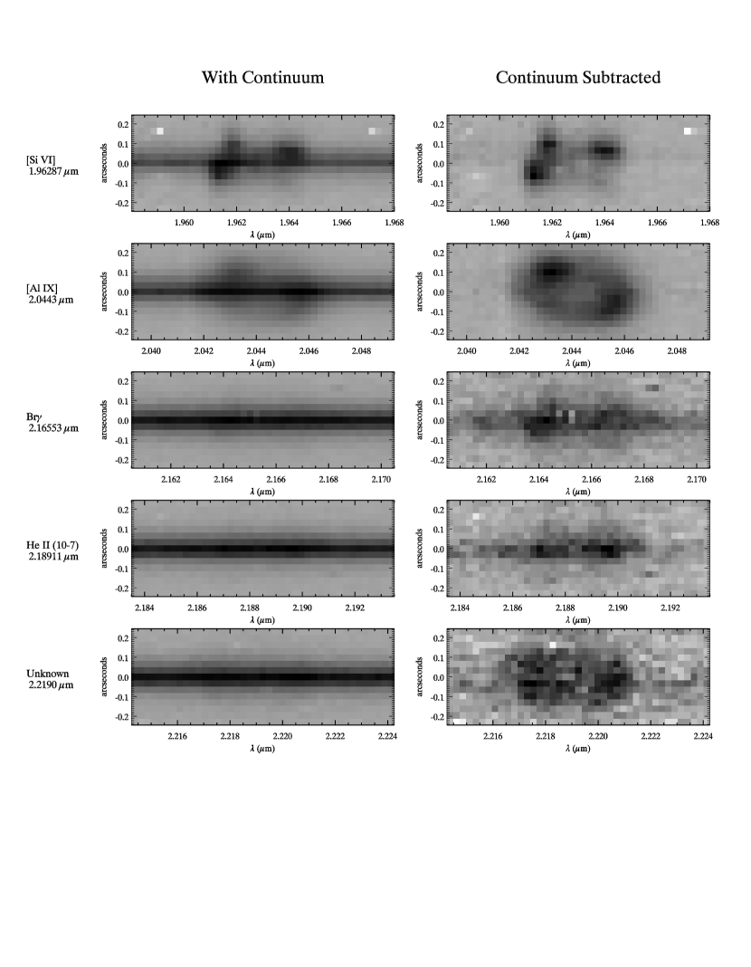
Figure 2: Two dimensional OSIRIS spectra from 2006. The left hand column shows the original spectra, the right hand column shows the continuum–subtracted spectra The bright [Si VI] and [Al IX] lines show a striking difference in morphology.

V723 Cas proved to be a bright continuum source throughout our observations. We do not detect continuum emission in the nebular region. The continuum of a classical nova long after outburst is dominated by light from the accretion disk as evidenced by studies of eclipsing systems (Horne 1985). As such, it is not resolved and thus represents the PSF of the data. In order to better study the extended emission line regions, we removed the point–source continuum from the data cube. The ability to separate the 3D data cube into a 2D image at each wavelength makes the continuum removal process straightforward. 1) The integrated spectrum of the source is examined to determine a spectral range over which there are no emission lines and no atmospheric features. 2) A continuum image is created by median–combining the pure continuum wavelength channels. Note that this continuum image has the same $x$ and $y$ dimensions as the data cube. 3) A 1D spectrum is extracted from a $3\times 3$ spaxel region of the object data cube centered on the peak of the continuum image. The 9–spaxel extraction gives both a high signal–to–noise ratio and averages out the impact of a bad data cube element. 4) An interpolation is performed over the emission features in the extracted spectrum and 5) the emission line–free continuum is smoothed with a boxcar 5 wavelength channels wide. 6) At each wavelength, the value of the modified continuum spectrum is used to scale the peak of the source in the continuum image. The scaled continuum image is subtracted from each wavelength channel of the data cube. The result is demonstrated in Figure 2 as the 2D spectrum with the continuum removed accentuates the extended emission and shows little residual emission at the position of the point–like continuum. The subtraction process does not require PSF modeling or fitting and is therefore robust. We note however that as V723 Cas fades, the continuum subtraction residuals are larger relative to the shell emission in our later epoch observations.

4 Results

4.1 NIRSPEC

The NIRSPEC spectrum of V723 Cas shows that it is a strong emission line source, some 3285 days after discovery. As Figure 1 shows, the most prominent lines are Pa$\alpha$, [Si VI] 1.96 $\micron$, [Al IX] 2.04 $\micron$, Br$\gamma$, [Ca VIII] 2.32 $\micron$, and [Si VII] 2.48 $\micron$. The list of identified lines appears in Table 2. Nearly all lines are double–peaked, indicating expansion as expected. The brightest emission lines were targeted for OSIRIS follow–up.

4.2 OSIRIS

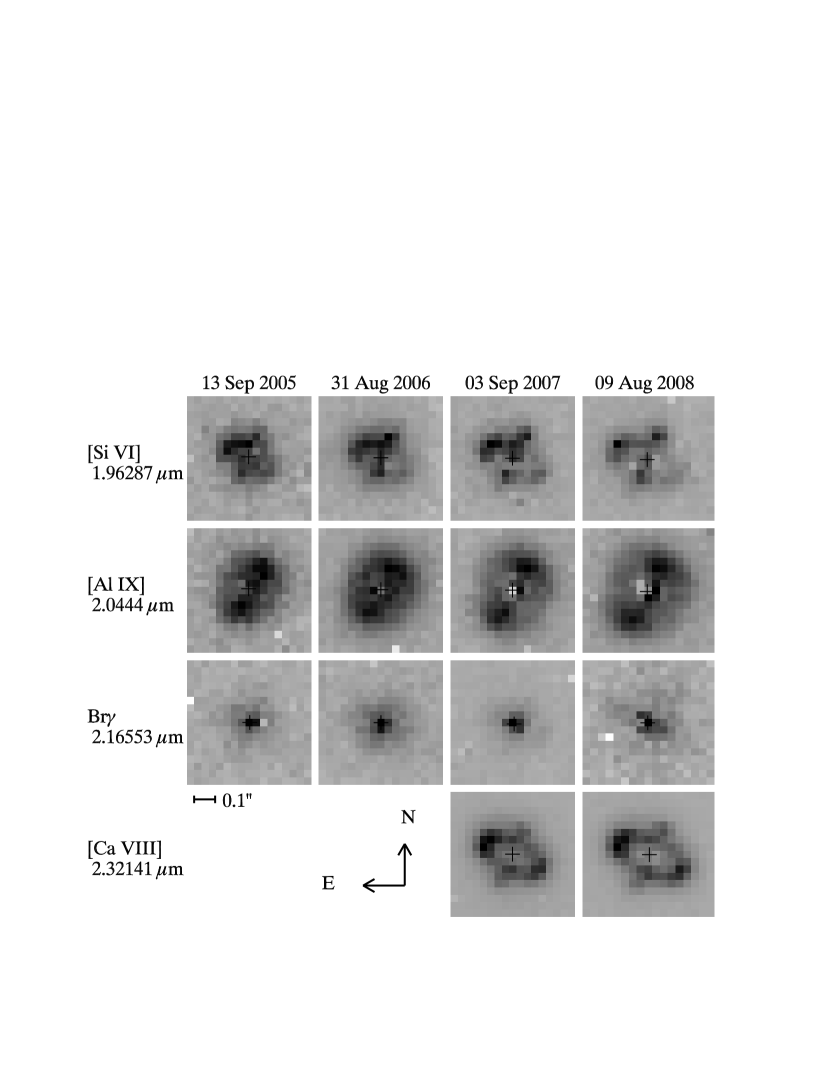
Figure 4: Narrowband images of V723 Cas of various emission lines show different morphologies. Each row holds images from one species and each column contains images for one epoch. The continuum has been subtracted from each image. Images are normalized but each image has its own linear stretch to accentuate features. The passbands for the [Si VI], [Al IX], Br$\gamma$, and [Ca VIII] images are $0.0055~{}\micron$, $0.00775~{}\micron$, $0.0055~{}\micron$, and $0.00725~{}\micron$ respectively.

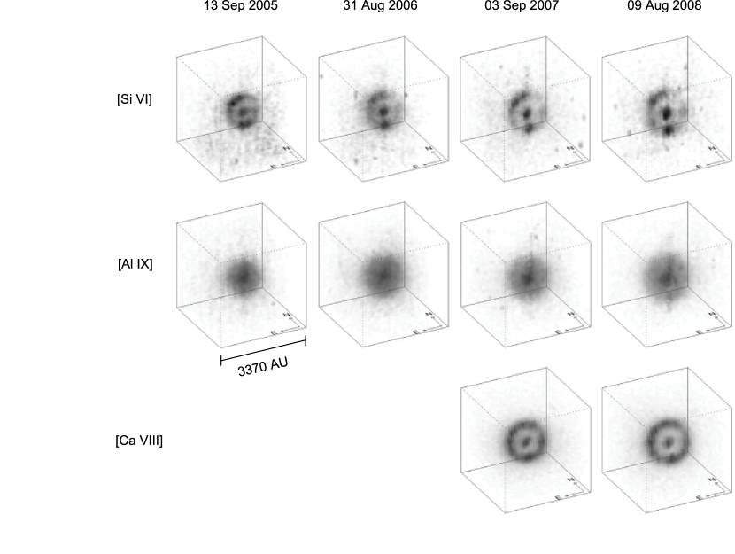
Figure 7: Face–on view of V723 Cas in various emission features after the data were remapped to 3 spatial dimensions. The cubes have been rotated as described in §4.2.5 and are 3370 AU on a side. The solid lines of the cube outline are in the foreground, the dotted lines are in the background. Both [Si VI] and [Ca VIII] show a distinct torus of emission whereas [Al IX] has a filled–in shell morphology. In all cubes, the bright spot in the center is due to the polar emission.

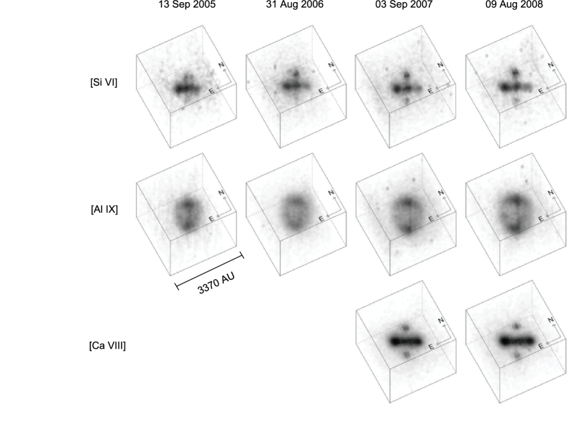
Figure 8: Edge–on view of V723 Cas in various emission features after the data were remapped to 3 spatial dimensions. The cubes have been rotated as described in §4.2.5 and are 3370 AU on a side. The solid lines of the cube outline are in the foreground, the dotted lines are in the background. Here, the torus of emission of [Si VI] and [Ca VIII] is clearly separated from the polar emission. The [Al IX] polar emission is clearly seen.

The nova shell of V723 Cas is resolved in both the spatial and wavelength dimensions of the 3D data cube. The high spatial resolution data reveal a complex structure of the nova ejecta. In order to highlight certain features of the nova ejecta, we display the data in various forms. These include 1D spectroscopy (Figure 1), 2D spectroscopy (Figure 2), narrowband imaging (Figure 4), and 3D spatial–velocity (Figure 7 and Figure 8).

4.2.1 1D Spectroscopy

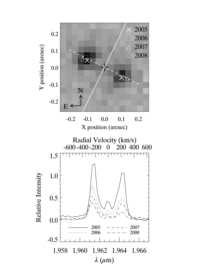
Figure 3: Constant expansion velocity. The upper panel shows the centroid of emission at the zero velocity of [Si VI] for four epochs superimposed upon the [Si VI] image from 2005. The passband of the image is $0.00050~{}\micron$. The black ”plus” marks the position of the subtracted continuum, the white dashed line has the slope of the best fit line through the data points, and the white solid line is perpendicular to the dashed line and shows the line along which the spectra in the lower panel were measured. The lower panel shows the spectra of V723 Cas centered on the [Si VI] line.

The OSIRIS data cube can be integrated over both spatial dimensions to create the equivalent of a slit spectrum of V723 Cas. This allows a direct comparison with the NIRSPEC spectrum as shown in Figure 1 and Table 2. For Figure 1 we extracted an $11~{}\times~{}11$ spaxel box centered on the continuum source to approximate the $0\farcs 38$ slit used in the NIRSPEC spectrum. It is evident that [Al IX] is stronger compared to [Si VI] in 2005 than in 2004. Rudy et al. (2002) detected a weak [Al IX] line with a flux ratio compared to that of [Si VI] of $0.002~{}\pm~{}0.0015$ in 1999 and $0.005~{}\pm~{}0.0015$ in 2000. Thus, over the 1999–2008 span of observations the [Al IX] has strengthened significantly each year with respect to [Si VI]. The OSIRIS spectral coverage is limited compared to that of NIRSPEC so certain lines, such as [Si VII] 2.48 $\micron$ and Br$\delta$ are not included in our spatially resolved study. The spectra from the OSIRIS Kn3 filter and NIRSPEC did include features seen in Rudy et al. (2002), including He II (10–7) 2.1882 $\micron$, [Ti VII] 2.2050 $\micron$, and an unidentified line at near 2.2188 $\micron$. While Rudy et al. (2002) ultimately found this line to be unidentified, they did offer [Fe III] 2.2178 $\micron$, hereafter [Fe III], as a possible source. Emission from [Fe III] does appear in OSIRIS data taken near the Galactic center (Ghez & Do, private communication) and our analysis shows the unidentified line center to be 2.2190 $\micron$, a difference of 5 wavelength channels. For this reason, we concur with Rudy et al. (2002) that this line is not due to [Fe III]. An important result of the spectral analysis is that the radial velocity of the nova shell remains constant over our 5 years of observation (see Figure 3). We use this fact in §4.2.4, to determine the distance to V723 Cas via expansion parallax.

4.2.2 Imaging

A useful feature of integral field instrumentation is the capability to create images using a customized bandpass tailored to any feature of the spectrum selected after the data have been acquired. Figure 4 shows custom narrowband images of selected emission features in the resolved nova ejecta from the coronal lines of [Si VI], [Al IX], [Ca VIII] and the hydrogen recombination line, Br$\gamma$. Most noticeable is the difference between the [Al IX] emission when compared to the [Si VI] and [Ca VIII] features. The [Al IX] feature is relatively smooth and consistent with a prolate spheroid shell. The other features have an equatorial torus and polar nodules similar to that seen in other novae ejecta such as DQ Her (Mustel & Boyarchuk, 1970), HR Del (Harman & O’Brien, 2003),V1974 Cyg (Paresce et al., 1995), and FH Ser (Gill & O’Brien, 2000). For [Si VI] and [Al IX], the ejecta expansion is evident over the four years of OSIRIS observations

4.2.3 2D Spectroscopy

IFS data can be presented in a conventional 2D format for the purpose of highlighting certain features and to enable comparison to long slit data of more conventional spectrometers. Figure 2 is a sampling of 2D spectra of selected bands from the 2006 OSIRIS data. The 2D spectra are produced by extracting a portion of the cube that would correspond to a slit–like region of interest if the slit were aligned north–south and $0\farcs 5$ in width. The intensity is summed in the $x$ spatial dimension (E–W) and then displayed as a function of wavelength versus the $y$ spatial dimension (N–S). In the left column of Figure 2, the spectra are shown with the continuum. In the right column, the point–like continuum has been subtracted. It is apparent that the [Al IX] emission is distinctive in its spatial–velocity structure. We note that the continuum subtracted data confirm that the coronal emission originates exclusively in the ejecta while the hydrogen recombination Br$\gamma$ line appears to come from both the ejecta and the central source. More clearly evident in the 2D spectra than in narrowband images, the extended portion of Br$\gamma$ and He II (10–7) appear to have a structure similar to that of [Si VI] and [Ca VIII]. In contrast, the unknown feature centered at 2.2190 $\micron$ is more like [Al IX] than [Si VI].

4.2.4 Distance

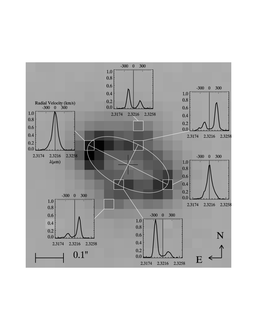
Figure 5: Spectra extracted from individual spaxels are shown overlaid on the [Ca VIII] image from 2007. This image is identical to that shown in Figure 4. The ellipse shows a circular torus inclined to the plane of the sky at 62$\arcdeg$. Spectra from the regions where the ellipse intersects the major axis of the ellipse show no net velocity. Spectra from the regions where the ellipse intersects the minor axis of the ellipse show primarily blue–shifted emission along the SE edge and primarily red–shifted emission along the NW edge. Emission from the regions above NW edge and below the SE edge of the ellipse have the opposite velocity sense of the regions along the minor axis of the ellipse. This emission is attributed to polar caps of emission. The black ”plus” sign denotes the location of the subtracted continuum.

The spatially resolved IFS 3D data provide all the necessary information for an accurate distance determination. Angular expansion and radial velocity measurements can be derived from the same dataset, an advantage over methods that use different measurements acquired at different times. We demonstrate this in Figure 5, where we have overplotted spectra at various locations of the [Ca VIII] feature from 2007. The 3D data cube allows us to spectroscopically confirm that the apparent ellipse of emission is consistent with an inclined circular torus with polar nodules perpendicular to the torus. We have overlaid an ellipse on the image to guide the reader’s eye. Spectra at positions along the major axis of the torus have zero radial velocity; therefore, they are moving in the plane of the sky. At positions along the minor axis of the torus, the spectra have double–peaked emission, with the SE portion more blueshifted and the NW portion more redshifted. The spectra at positions away from the torus have the opposite velocity direction as the spectra on the torus, indicating a polar nodule structure. We make use of our knowledge of the morphology and inclination of the system to accurately determine a distance to V723 Cas. Rather than assume spherical symmetry of the nebula with Hubble flow properties, the distance analysis in this study uses the equatorial torus portion of the expanding ejecta and is based on the assumption that the torus is circular, or azimuthally symmetric.

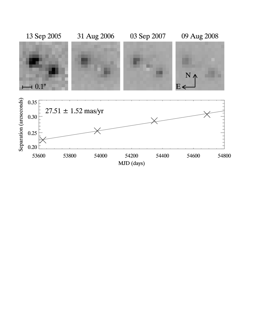
Figure 6: Expansion of the torus of emission is shown in both images and a plot. The upper panel shows the zero velocity images of [Si VI] (as in Figure 3) at each of our four epochs. The continuum has been removed from each image. Images are normalized and displayed with the same linear stretch. The lower panel plots the measured separation of the two emission peaks as a function of time. Each year, the torus expands just less than one 35 mas spaxel.

We create a zero velocity image for each emission feature by selecting the wavelength channel or channels that correspond to the central wavelength of each emission feature. Reconditi & Oliva (1993) give the wavelength of [Si VI] to be $1.96287~{}\pm~{}1.0~{}\micron$. This corresponds to wavelength channels 31 and 32 in our Kn1 data cubes. We determine the angular expansion rate by measuring the centroids of emission in the zero velocity image for [Si VI], or in other words, the cross section of the torus that is expanding perpendicular to our line of sight. In a zero velocity image, the equatorial torus of emission appears as two peaks on opposite sides of the continuum location and moves purely in the plane of the sky (see Figure 6). We use only [Si VI] because its morphology lends itself to this analysis and the observations of [Si VI] cover a four year span. We do not include [Ca VIII] in the distance analysis because we have only two epochs of observations and we do not assume that the two lines are perfectly coincident nor co–moving. We fit the angular separation of the two emission peaks in the zero velocity image of each epoch by the method of linear least squares to determine an angular expansion rate, $\phi~{}=~{}27.51~{}\pm~{}1.52~{}mas~{}yr^{-1}$ as seen in Figure 6. We note that this determination does not depend on the assumed time of outburst (t₀). From the zero velocity emission peaks, we measure the position angle of the torus to be 63$\fdg 7~{}\pm~{}$2$\fdg$0.

The high spatial resolution of the IFS data allow a velocity measurement to be made at precise positions of the expanding torus of material. We measure the radial velocity along a line perpendicular to the line defined by the two zero velocity image centroids (see the solid white line in the upper panel of Figure 3). The radial velocity line is nearly coincident to the projection of the polar nodules onto the plane of the sky so care must be taken when extracting the spectrum. Here, the 3D data cube allows us to separate the emission in velocity space. As seen in Figure 5, the northwest polar nodule is more blueshifted, while the northwest portion of the equatorial torus is more redshifted. In a similar way, the southeast polar nodule is more redshifted, while the southeast portion of the equatorial torus is more blueshifted. We extract only the spectrum arising from the equatorial torus for our distance determination.

Our extracted [Si VI] spectrum is double–peaked as shown in Figure 3. Because we measure the angular expansion rate of the two emission peaks of the zero velocity image from each other, we must also measure the total velocity separation, $v_{r}$, of the red– and blue–shifted emission peaks for each epoch. We find $v_{r}~{}=~{}443.3~{}\pm~{}12.0~{}km~{}s^{-1}$. The relation of the expansion velocity, $v_{exp}$, to the radial velocity is given by:

$$v_{exp}=v_{r}sin~{}i$$ (1)

where $i$ is the inclination of the system defined such that edge–on is $i~{}=~{}90\arcdeg$. We measure the semi–major and semi–minor axes of an ellipsoidal projection of the circular torus onto the image plane to determine an inclination of $62\fdg 0~{}\pm~{}1\fdg 5$. Figure 5 shows an ellipse graphic using the above parameters overlaid on the [Ca VIII] image taken in September 2007. By Equation 1, $v_{exp}~{}=~{}502.1~{}\pm~{}13.6~{}km~{}s^{-1}$. The measured constant velocity over the 5 years of observations is consistent with a freely expanding torus unencumbered by shock encounters with pre–outburst or interstellar material.

Using our measured angular expansion rate and expansion velocity, we can calculate the distance to V723 Cas via expansion parallax:

$$d[kpc]=0.211\frac{v_{exp}[km~{}s^{-1}]}{\phi[mas~{}yr^{-1}]}$$ (2)

By Equation 2, the distance to V723 Cas is $3.85^{+0.23}_{-0.21}~{}$kpc. We consider 3 main sources of errors due to: 1) uncertainty in the angular expansion rate, 2) line fitting, and 3) inclination uncertainty. The error in the angular expansion rate accounts for most of the error in distance (${}^{+0.22}_{-0.20}~{}kpc$) while the other two sources of error account for less than $\pm~{}0.01~{}kpc$ each. A summary of data used to determine the expansion parallax is found in Table 3.

By comparison, distance estimates vary widely in the literature. Evans et al. (2003) estimate the distance to be 4.0 kpc employing a combination of methods that yield a range of distances from $3.5$ to $4.2~{}kpc$. Ness et al. (2008) assume that the absolute magnitudes of HR Del and V723 Cas are identical to find a distance, then average this with other distances in the literature to yield $2.7^{+0.4}_{-0.3}~{}$kpc. The expansion parallax method in this study provides the most accurate determination of the distance to V723 Cas. This distance may help provide an improvement in the calibration the MMRD relationship for slow novae. Our distance determination of 3.85 kpc is also consistent with the WD mass estimate from Evans et al. (2003) of 0.67 M_☉.

4.2.5 3D Projection

The OSIRIS IFS 3D data cube is a measurement of intensity as a function of spatial extent and wavelength. The 3 axes of the cube can be converted into units of distance in order to visualize the true shape of the nova ejecta. The units of the two spatial dimensions are converted from angle on the sky to length based on the measured distance to V723 Cas. The extent of the nova shell in the line of sight dimension can be computed from its expansion velocity. For our 3D spatial cubes, we chose 25 spatial lenslets per side. At a distance of 3.85 kpc, this gives 3370 AU. For our visualization, we elected not to interpolate over spectral pixels such that we rounded the calculated number of spectral channels in 3370 AU down to the nearest even integer. Table 4 shows this conversion in units of number of spectral channels in 3370 AU for a given spectral feature and date. The conversion factor decreases with time since the measured velocity remains constant as the distance traveled by the torus increases from year to year.

A data cube of 3 spatial dimensions is rendered for the brightest spectral features using the volume rendering capabilities of IDL in Figure 7 and Figure 8. The cubes are 3370 AU per side and have a unique linear stretch to accentuate details; however, all features are fading with time. As noted earlier, the continuum from the central source has been removed. Once we have remapped the data cube to spatial 3D, we can rotate the cube to show the equatorial and polar emission more clearly. We start with the image projection of the data cube such that $x$ corresponds to east, $y$ to north, and $z$ (formerly $\lambda$) into the page. First we rotate the cube about the $z$ axis by the complement of the position angle ($26\fdg 3$) such that the projected major axis of the equatorial torus is now horizontal. Next we define a modified $x$ axis ($x^{\prime}$) along the projected major axis of the equatorial torus. To get the face–on view (Figure 7), we rotate about the $x^{\prime}$ axis by the inclination of $62\arcdeg$. To get the edge–on view (Figure 8), we rotate about the $x^{\prime}$ axis in the opposite direction by the complement of the inclination ($-28\arcdeg$).

In the face–on view (Figure 7), the torus structure is clearly visible and we can see knots in the torus in [Si VI] and [Ca VIII]. The circular torus of emission confirms the validity of our visualization technique as our distance determination assumed a circular torus. The 3D visualization emphasizes the dramatic difference between the structure of [Al IX] feature, a prolate spheroid, and the other features, an equatorial torus with polar nodules. The bright spot near the center of each cube is the polar emission. As the features fade, residuals of the continuum subtraction become visible as a faint vertical line of emission passing through the center of the nebula.

In the edge–on view (Figure 8), again we see striking differences in the morphologies of the features. The polar nodules are visible in all cubes while any sign of an equatorial torus is absent from the [Al IX] cubes.

The spatial 3D rendering allows the direct measurement of the polar–to–equatorial axial ratio of the nebula without dependence on viewing angle. Based on data from 2008, the polar regions were separated by 1670 AU while the equatorial region spanned only 1270 AU. Thus, the axial ratio is relatively small, $1.32~{}\pm~{}0.05$.

5 Discussion

Morphological differences are not new in nova ejecta. Using archival plates of DQ Her, Mustel & Boyarchuk (1970) found an equatorial band and polar condensations in emission attributed to H$\alpha$ while emission attributed to [O III] showed no equatorial feature. Harman & O’Brien (2003) resolved an hourglass shaped shell in HR Del with an equatorial torus using HST narrow band imaging. They also found morphological differences between H and [O III] emission and point out the observations can critically constrain our knowledge of the history of convection during the TNR. In addition to shell morphology differences between emission lines, HR Del has much in common with V723 Cas in terms of speed class, orbital parameters, and coronal emission. One difference is the polar–to–equatorial axial ratio of the shell. HR Del has a large axial ratio of $1.75~{}\pm~{}0.15$ for the prolate ellipsoidal shell that supports the shell shape rate of decline (SSRD) relationship proposed by Slavin, et al. (1995). However, the SSRD relationship does not hold as strongly for V723 Cas, one of the slowest novae on record, with its smaller axial ratio of $1.32~{}\pm~{}0.05$. We note that axial ratio determined from direct imaging is highly dependent on the viewing angle and that future studies with IFS instruments could more accurately determine any relation of shell shape with other nova parameters.

There are several possible explanations for the morphological difference between [Al IX] and [Si VI] and [Ca VIII]. The first is the shell is chemically homogenous, but contains ”clumps” of denser material embedded within a sparser medium. This interpretation is typically used to resolve how emission from low– and high–ionization potential species can co–exist (see $e.g.$ Lyke et al., 2001, 2003). While we do not see uniformly distributed clumps of dense material, the equatorial torus could provide some photon shielding. In fact, the ionization potentials of [Ca VIII] and [Si VI] are lower than that of [Al IX] ($147~{}eV$ and $205~{}eV$ versus $330~{}eV$ respectively), but we do not see an inner equatorial torus of [Al IX] as one might expect from this interpretation.

A second description may be that the ejecta are inherently homogeneous but there are two spatially distinct populations of electrons that permit lines from different ions to dominate the emission. Due to the limited wavelength range of OSIRIS and the resulting lack of the necessary combination of emission lines, we are unable to determine the electron temperatures or densities within the distinct regions of the V723 Cas ejecta. Previous studies and our NIRSPEC spectra presented here lacked the spatial resolution to differentiate between emission regions; thus, any determinations of electron properties are averaged over the entire shell. For these reasons, we are unable to adequately test the existence of multiple electron populations.

The most intriguing interpretation considers that the shell may not be homogeneous and the observed differences are a result of separate ejection events, perhaps from different regions of the WD. Lynch et al. (2008) explain the pronounced second brightening of the recent nova V2362 Cyg as a separate TNR ejection event and Evans et al. (2003) suggested that the multiple peaks in the visual light curve of V723 Cas may be the result of multiple mass ejection events. If so, multiple mass ejection events may be common because many novae have had multiple peaks in the visual light curves during their early evolution. A possible cause of multiple TNR ejection events may be that the TNR does not occur uniformly over the surface of the WD.

As the H–rich material accretes to the WD via a disk near the orbital plane, it is likely the accreted material is concentrated near the equator of the WD. Therefore, it is reasonable to assume that the TNR occurs first near the equatorial regions of the WD. If so, then the mass is ejected mostly in the orbital plane and is subjected to shaping during the common envelope (CE) phase. The structure of the V723 Cas ejecta is similar to the fast nova V1974 Cyg, with its well–defined equatorial torus (Paresce et al., 1995). The IR spectrum of V1974 Cyg (Wagner & DePoy, 1996) exhibits many of the same emission features as in V723 Cas, but at much higher expansion velocities. Paresce et al. (1995) discuss the ejecta may have been shaped by the CE phase with binary orbit depositing angular momentum into the CE, thereby enhancing the density into the equatorial plane. If the fast moving ejecta of V1974 Cyg was shaped into an equatorial torus by its CE phase, it is likely the binary orbit shaped the much slower ejecta of V723 Cas during its CE phase. The energy from the TNR in the equatorial region may heat the higher latitudes of the WD, eventually triggering additional TNR events. If so, the subsequent mass ejections may be concentrated towards the poles. Any observations of abundance gradients in nova ejecta may help constrain the knowledge of the history of convection during the TNR (Starrfield, et al., 2008). Lloyd et al. (1997) modeled the CE phase and showed that slower novae are more likely to have the envelope ejected in the plane of the binary orbit. However they also predict very little mass loss in the polar direction. Porter et al. (1998) enhanced the CE model of Lloyd et al. (1997) by including envelope rotation which can produce more prolate shaped ejecta. Our observations of V723 Cas should be able to help constrain models such as these to learn more about the pre–outburst accretion phase and material mixing on the WD.

If an equatorial torus is a result of the CE phase, the inclination of the torus can be assumed to be the same as the inclination of the binary orbit. For V723 Cas, we measure the inclination to be $62\fdg 0~{}\pm~{}1\fdg 5$. Roche geometry cannot produce an eclipse light curve at this inclination (Horne, 1985); thus, the sawtooth pattern in the light curve with orbital period of $0\fd 693265$ measured by Goranskij et al. (2007) is likely due to heating effects of the secondary surface that faces the WD. We would expect the amplitude of the light curve variations in V723 Cas to diminish with time as the radiation from the primary returns to quiescence.

6 Conclusions

We have presented IFS observations of V723 Cas with unprecedented spatial resolution in the IR. These data allow us to remove the point–like continuum and create custom narrowband ”filter” images of coronal emission features that allow us to see 2 distinct ejecta morphologies. Furthermore, our dataset allows us to determine a highly accurate distance of $3.85^{+0.23}_{-0.21}~{}$kpc. We have used this distance to convert our $x-y-\lambda$ data cubes into $x-y-z$ spatial data cubes that allow us to compare the true shapes various emission lines. The morphological differences are likely due to separate ejection events possibly due to an uneven TNR combined with some self–shielding of X–rays by the equatorial torus. We anticipate that these V723 Cas data and future IFS data of classical novae will help constrain models that attempt to describe the nature of the outburst.

Figure 1: One dimensional spectra for NIRSPEC (NS) and OSIRIS (OS) from 2004 through 2008. We note that the [Al IX] feature gets stronger as compared to the [Si VI] feature with time. Relative flux ratios are given in Table 2.

Table 1: Observational Details

UT Date	Days since	Instrument	Filter	$\lambda$ Range	exp time	WFS Rate
	outburst			($\micron$)	(s)	(Hz)
2004 Aug 22	3285.6	NIRSPEC	N–3	1.1–1.3	300	n/a
2004 Aug 22	3285.6	NIRSPEC	N–7	1.9–2.2	300	n/a
2004 Aug 22	3285.6	NIRSPEC	N–7	2.2–2.6	300	n/a
2005 Sep 13	3672.4	OSIRIS	Kn1	1.955 – 2.055	900	300
2005 Sep 13	3672.4	OSIRIS	Kn2	2.036 – 2.141	900	300
2005 Sep 13	3672.4	OSIRIS	Kn3	2.121 – 2.229	900	300
2006 Aug 31	4024.4	OSIRIS	Kn1	1.955 – 2.055	1800	300
2006 Aug 31	4024.4	OSIRIS	Kn3	2.121 – 2.229	1800	300
2007 Sep 03	4392.5	OSIRIS	Kn1	1.955 – 2.055	3600	800
2007 Sep 03	4392.5	OSIRIS	Kn3	2.121 – 2.229	3600	800
2007 Sep 03	4392.5	OSIRIS	Kn5	2.292 – 2.408	1800	800
2008 Aug 09	4733.5	OSIRIS	Kn1	1.955 – 2.055	5400	800
2008 Aug 09	4733.5	OSIRIS	Kn3	2.121 – 2.229	3600	800
2008 Aug 09	4733.5	OSIRIS	Kn5	2.292 – 2.408	1800	800

Table 2: Relative Fluxes

Wavelength		F/F([Si VI])
($\micron$)	Identification	2004	2005	2006	2007	2008
1.87561	Pa$\alpha$	1.596	$\cdots$	$\cdots$	$\cdots$	$\cdots$
1.94509	Br8	0.194	$\cdots$	$\cdots$	$\cdots$	$\cdots$
1.96287	[Si VI]	1.000	1.000	1.000	1.000	1.000
2.03788	He II 15–8	$\cdots$	0.065	$\cdots$	$\cdots$	$\cdots$
2.0443	[Al IX]	0.342	0.786	1.022	1.106	1.213
2.0581	He I	0.017	$\cdots$	$\cdots$	$\cdots$	$\cdots$
2.0996	?	0.022	0.062	$\cdots$	$\cdots$	$\cdots$
2.1156	He I	0.015	$\cdots$	$\cdots$	$\cdots$	$\cdots$
2.16553	Br$\gamma$	0.091	0.390	0.381	0.560	0.886
2.18911	He II 10–7	0.048	0.142	0.221	0.248	0.388
2.206	[Ti VII]	0.027	0.067	0.049	0.099	0.071
2.2190	?	0.050	0.097	0.165	0.185	0.142
2.32141	[Ca VIII]	3.200	$\cdots$	$\cdots$	5.519	6.144
2.34704	He II 13–8	0.021	$\cdots$	$\cdots$	$\cdots$	$\cdots$
2.4807	[Si VII]	4.111	$\cdots$	$\cdots$	$\cdots$	$\cdots$

Table 3: [Si VI] Expansion Parameters

UT Date	MJD	Separation	Separation	$v_{exp}$
		($\arcsec$)	(AU)	($km~{}s^{-1}$)
2005 Sep 13	53626.4	0.2273	875	489.5
2006 Aug 31	53978.4	0.2556	984	491.3
2007 Sep 03	54346.5	0.2866	1103	512.0
2008 Aug 09	54687.5	0.3061	1178	515.5

Table 4: Data Cube Spectral Channel to Spatial Extent Conversion

Feature	2005	2006	2007	2008
[Si VI]	46	42	38	34
[Al IX]	48	44	40	36
[Ca VIII]	$\cdots$	$\cdots$	46	42

References

- Chochol & Pribulla (1997) Chochol, D., & Pribulla, T., 1997., Contributions of the Astronomical Observatory Skalnate Pleso, 27, 53.
- Evans et al. (2003) Evans, A., et al., 2003, AJ, 126, 1981.
- Gehrz et al. (1998) Gehrz, R. D., Truran, J. W., Williams, R. E., Starrfield, S., 1998, PASP, 110, 3.
- Gehrz et al. (1992) Gehrz, R. D., Grasdalen, G. L., Hackwell, J. A., & Jones, T. W., 1992, in The Encyclopedia of Physical Science and Technology, Vol. 2 (New York: Acadamic Press), 125.
- Gill & O’Brien (2000) Gill, C. D., & O’Brien, T. J., 2000, MNRAS, 314, 175.
- Goranskij et al. (2007) Goranskij, V. P., et al., 2007, Astrophysical Bulletin, 62, 125–146.
- Harman & O’Brien (2003) Harman, D. J. & O’Brien, T. J. 2003, MNRAS, 344, 1219.
- Heywood et al. (2005) Heywood, I., O’Brien, T. J., Eyres, S. P. S., Bode, M. F., Davis, R. J., 2005, MNRAS, 362, 469.
- Hirosawa et al. (1995) Hirosawa, K., Yamamoto, M., Nakano, S., Kojima, T., Iida, M., Sugie, A., Takahashi, S., Williams, G. V., 1995, IAU Circ., 6213.
- Horne (1985) Horne, K., 1985, MNRAS, 213, 129.
- Hutchings (1972) Hutchings, J. B., 1972, MNRAS, 158, 177.
- Iijima (2006) Iijima, T., 2006, A&A, 451, 563.
- Krabbe et al. (2004) Krabbe, A., Gasaway, T., Song, I., Iserlohe, C., Weiss, J., Larkin, J. E., Barczys, M., & Lafreniere, D. 2004, Proc. SPIE, 5492, 1403.
- Krautter et al. (2002) Krautter, J., et al., 2002, AJ, 124, 2888.
- Larkin et al. (2006) Larkin, J., et al., 2006, Proc. SPIE, 6269, 42.
- Lloyd et al. (1997) Lloyd, H. M, O’Brien, T. J., Bode, M. F., 1997, MNRAS, 284, 137.
- Lyke et al. (2001) Lyke, J. E., et al. 2001, AJ, 122, 3305.
- Lyke et al. (2003) Lyke, J. E., et al. 2003, AJ, 126, 993.
- Lynch et al. (2008) Lynch, D. K., et al., 2008, AJ, 136, 1815.
- McLean et al. (1998) McLean, I. S., et al., 1998, Proc. SPIE, 3354, 566.
- Mustel & Boyarchuk (1970) Mustel, E. R., & Boyarchuk, A. A., 1970, Ap&SS, 6, 183.
- Ness et al. (2008) Ness, J.-U., Schwarz, G., Starrfield, S., Osborne, J. P., Page, K. L., Beardmore, A. P., Wagner, R. M., Woodward, C. E., 2008, AJ, 135, 1328.
- Ohshima et al. (1995) Ohshima, O., et al., 1995, IAU Circ., 6214.
- Paresce et al. (1995) Paresce, F., Livio, M., Hack, W., Korista, K., 1995, A&A, 299, 823.
- Porter et al. (1998) Porter, J. M., O’Brien, T. J., Bode, M. F., 1998, MNRAS, 296, 943.
- Reconditi & Oliva (1993) Reconditi, M., & Oliva, E., 1993, A&A, 274, 662.
- Rudy et al. (2002) Rudy, R. J., Venturini, C. C., Lynch, D. K., Mazuk, S., Puetter, R. C., 2002, ApJ, 573, 794.
- Slavin, et al. (1995) Slavin, A. J., O’Brien, T. J., Dunlop, J. S., 1995, MNRAS, 276, 353.
- Starrfield, et al. (2008) Starrfield, S., Iliadis, C., Hix, W. R. in Classical Novae, eds. Bode, M. F. & Evans, A., [New York: Cambridge University Press].
- Wagner & DePoy (1996) Wagner, R. M., & DePoy, D. L., 1996, ApJ, 467, 860.
- Wizinowich et al. (2006) Wizinowich, P. L., et al., 2006, PASP, 118, 297.