Analytical Solutions for the Equilibrium states of a Swollen Hydrogel Shell and an Extended Method of Matched Asymptotics

Abstract

A polymer network can imbibe water, forming an aggregate called hydrogel, and undergo large and inhomogeneous deformation with external mechanical constraint. Due to the large deformation, nonlinearity plays a crucial role, which also causes the mathematical difficulty for obtaining analytical solutions. Based on an existing model for equilibrium states of a swollen hydrogel with a core-shell structure, this paper seeks analytical solutions of the deformations by perturbation methods for three cases, i.e. free-swelling, nearly free-swelling and general inhomogeneous swelling. Particularly for the general inhomogeneous swelling, we introduce an extended method of matched asymptotics to construct the analytical solution of the governing nonlinear second-order variable-coefficient differential equation. The analytical solution captures the boundary layer behavior of the deformation. Also, analytical formulas for the radial and hoop stretches and stresses are obtained at the two boundary surfaces of the shell, making the influence of the parameters explicit. An interesting finding is that the deformation is characterized by a single material parameter (called the hydrogel deformation constant), although the free-energy function for the hydrogel contains two material parameters. Comparisons with numerical solutions are also made and good agreements are found.

AMS Subject Classification: 74F20, 74B20, 34E15, 34B15

1 Introduction

Gels, known as a cross-linked solution,[12] consist of a solid three-dimensional network of polymer that spans the volume of a liquid medium and imbibes the solvent molecules through surface tension effects. When the solvent happens to be water, the aggregate is called hydrogel (e.g. edible jelly), which can undergo large and reversible volumetric deformation by absorbing or expelling water in response to various external stimuli (e.g. temperature, physical or chemical stimuli like light and pH). It undergoes a homogeneous deformation without external mechanical constraint, but an inhomogeneous and anisotropic one under external constraints (often present in practice).

This paper deals with a core-shell structure, with a shell of gel fixed to a hard core of another material (like metal or another polymer), which defines an inner boundary of the network. Due to the good properties such as stability, ease of synthesis, thermalsensitivity and biocompatible nature etc., such a hydrogel shell has various promising applications including drug delivery,[8, 21, 22] medical devices,[16] bioseparation[20] and catalysis.[2, 3] Some experiments[1, 7] have been performed on such a structure in recent years. It was found that there exists a density fluctuation within the network which indicates the spatial inhomogeneity. Sometimes, the partial detachment of the shell, which means the large stress at the inner surface due to the strong swelling, was observed. Thus a good understanding of equilibrium swelling states is of crucial importance. However, few analytical results exist for such inhomogeneous swelling and consequently there lacks the interpretation of the influence of the material parameters on the deformation.

Equilibrium theories of heterogeneous substances date back to Gibbs,[15] who formulated a theory for the inhomogeneous equilibrium state of large deformation of an elastic solid in a solvent. Recently extensive studies have concentrated on the swelling of gels.[9, 10, 11] Particularly based on the field theory of Gibbs[15] and the poroelasticity theory of Biot,[4, 5] Hong et al.[19] formulated a theory of couple mass transport and deformation in gels by considering both the mixing and stretching processes, leaving open the free-energy function. For the specific core-shell structure of hydrogel, Zhao et al.[27] and Hong et al.[18] adopted the free-energy function introduced by Flory and Rehner[14] and obtained some numerical results of the inhomogeneous swelling states, showing large stresses near the core-shell interface.

The present work is restricted to the equilibrium swelling states (i.e. the long-time limit) without considering kinetics, of which the deformation of the network is governed by a boundary-value problem. The object of this paper is to seek analytical solutions of radially symmetric deformations for such a core-shell structure, based on the existing model in Ref. hydrogelsuo1. Usually, it is very difficult to obtain analytical solutions for an inhomogeneous state of a hydrogel due to the nonlinearity caused by the large deformation. In the case of uniform swellings (the water concentration is uniformly distributed), a number of analytical solutions have been obtained.[23, 24, 25, 26] For the present problem, the water concentration is nonuniform, and as far as we know, analytical solutions for this type of problems are not available in literature.

Here we intend to construct the asymptotic solutions for the present problems. Identifying a small parameter in the governing equations, we analyze the deformations by perturbation methods. For the homogeneous deformation, by defining a hydrogel deformation constant $\alpha$ we can express the free stretch in a simple formula. For the general inhomogeneous deformation, we treat it as a boundary-layer problem of a nonlinear second-order variable-coefficient differential equation. It turns out that there is a boundary layer near the hard core, but the existing method of matched asymptotics does not work for the present problem. Here we introduce an extended method of matched asymptotics to construct the analytical solution. More specifically, this novel methodology involves the introduction of a transition region besides the usual inner and outer regions and using a series solution in this region.

This paper is arranged as follows. Section 2 briefly recalls the formulation of Zhao et al.[27] for the hydrogel in the equilibrium state. We then consider in section 3 the free-swelling deformation with no external mechanical constraint, and in section 4 we discuss a near free-swelling deformation with the fixed hoop stretch at the inner surface not far from the free stretch. Section 5 discusses a general inhomogeneous deformation without such a restriction on the fixed stretch, where an extended method of matched asymptotics is introduced to construct the analytical solution. Finally some conclusions are drawn.

2 Governing Equation

For the structure of a spherical shell, the spherical symmetric deformation of the hydrogel is fully specified by a function $r(R)$. In this section we briefly recall the formulation of Zhao et al.[27] for the hydrogel in the equilibrium state. The field equation is

$$\frac{ds_{r}}{dR}+2\frac{s_{r}-s_{\theta}}{R}=0,$$ (1)

where $s_{r},s_{\theta}$ are the nominal stresses in the radial and circumferential directions respectively.

We adopt the free energy function of the hydrogel first introduced by Flory and Rehner (see Ref. hydrogelpolymer2,hydrogelflory1) and follow the notations in Hong et al.[19]

$$W(\mathbf{F},C)= W_{s}(\mathbf{F})+W_{m}(C)$$ (2)

$$= \frac{1}{2}NkT[\lambda_{1}^{2}+\lambda_{2}^{2}+\lambda_{3}^{2}-3-2\log\lambda_{1}\lambda_{2}\lambda_{3}]$$

$$-\frac{kT}{v}\left[vC\log(1+\frac{1}{vC})+\frac{\chi}{1+vC}\right],$$

where $\mathbf{F}$ is the deformation gradient, $C$ is the nominal concentration of water (i.e. the number of the water molecules per reference volume in the current state), $N$ is the number of polymer chains per reference volume of dry network, $kT$ is the temperature in the unit of energy ($k$ is the Boltzmann’s constant), $\lambda_{1},\lambda_{2}$ and $\lambda_{3}$ are the three principal stretches, and $v$ is the volume per solvent molecule (water), $\chi$ is a parameter from the heat of mixing. The two dimensionless parameters $\chi$ and $vN$ vary in the ranges $0.1-0.5$ and $10^{-2}-10^{-5}$ respectively according to Zhao et al.[27] ($1/vN$ actually is the number of water molecules occupied the same volume of per polymer chain).

For a spherically symmetrical deformation, it is easy to deduce from (2) that

$$\frac{s_{\theta}}{NkT} =\lambda_{\theta}-\lambda_{\theta}^{-1}+\frac{\lambda_{\theta}\lambda_{r}}{vN}\left[\log\frac{vC}{1+vC}+\frac{1}{1+vC}+\frac{\chi}{(1+vC)^{2}}\right],$$ (3)

$$\frac{s_{r}}{NkT} =\lambda_{r}-\lambda_{r}^{-1}+\frac{\lambda_{\theta}^{2}}{vN}\left[\log\frac{vC}{1+vC}+\frac{1}{1+vC}+\frac{\chi}{(1+vC)^{2}}\right],$$

where $\lambda_{\theta}$ and $\lambda_{r}$ are respectively the stretches in the circumferential and radial directions, and $vC$ represents the change in volume of the gel, which are given by

$$\lambda_{\theta}=\frac{r}{R},\quad\lambda_{r}=\frac{dr}{dR},\quad vC=\lambda_{\theta}^{2}\lambda_{r}-1.$$ (4)

Substituting (3-4) into (1), a nonlinear second-order variable-coefficient differential equation for $r(R)$ arises, which will be solved analytically subjected to suitable boundary conditions.

In the reference configuration (a water-free and stress-free state), suppose that the hydrogel shell has the inner and outer radii $A$ and $B$ respectively. Suppose that in the current configuration (an equilibrium state immersed in water) the inner surface is attached with a rigid core and has the radius $r(A)=\lambda_{0}A$. At the outer surface it is supposed that $s_{r}(B)=0$ or $s_{\theta}(B)=0$.

Since the change in volume $vC$ is relatively large (see Figure 2(a) in Ref. hydrogelsuo1), we approximate the term $\log\frac{vC}{1+vC}$ by the Taylor expansion in terms of $\frac{1}{1+vC}$. Then, from $(\ref{eq2}-\ref{eq3})$ we have

$$\frac{s_{\theta}}{NkT} =\lambda_{\theta}-\lambda_{\theta}^{-1}-\frac{1-2\chi}{2vN}\frac{1}{\lambda_{\theta}^{3}\lambda_{r}}-\frac{1}{3vN}\frac{1}{\lambda_{\theta}^{5}\lambda_{r}^{2}}+\cdots,$$ (5)

$$\frac{s_{r}}{NkT} =\lambda_{r}-\lambda_{r}^{-1}-\frac{1-2\chi}{2vN}\frac{1}{\lambda_{\theta}^{2}\lambda_{r}^{2}}-\frac{1}{3vN}\frac{1}{\lambda_{\theta}^{4}\lambda_{r}^{3}}+\cdots.$$

We notice that a small parameter $vN$ appears in the equation, so we would like to take advantage of this by using perturbation methods to get approximate analytical solutions for the following three cases.

3 Explicit Solution for a Free-swelling Deformation

If the hydrogel swells freely with no external mechanical constraint, the deformation is homogeneous and isotropic, i.e. $\lambda_{r}=\lambda_{\theta}=\lambda_{free}=(vC_{free}+1)^{1/3}$, which can be obtained by solving $s_{r}=0$ (or equivalently $s_{\theta}=0$). Now, we shall deduce the explicit asymptotic solution.

Substituting $\lambda:=\lambda_{r}=\lambda_{\theta}$ into $(\ref{eq5})$ we arrive at

$$\lambda-\lambda^{-1}-\frac{1-2\chi}{2vN}\frac{1}{\lambda^{4}}-\frac{1}{3vN}\frac{1}{\lambda^{7}}+\cdots=0.$$ (6)

Since $vC_{free}$ is large, we also regard $\lambda$ as a large quantity. From the above equation we can see that the term to balance the third term, which is large due to the small parameter $vN$, is the first term $\lambda$. Thus, they should have the same order, which implies that to the leading order

$$\lambda=[(1-2\chi)/(2vN)]^{1/5}=:\alpha.$$ (7)

We call $\alpha$ to be the hydrogel deformation constant, as we shall see that this single parameter plays a dominant role for the deformation. Letting $\lambda=\alpha\tilde{\lambda}$ and seeking a perturbation expansion solution of $(\ref{eq6})$ in the form

$$\tilde{\lambda}=1+\alpha^{-1}\lambda_{1}+\alpha^{-2}\lambda_{2}+O(\alpha^{-3}),$$ (8)

where $\alpha$ is treated as a large parameter, we obtain the formula

$$\lambda_{free}=\lambda=\alpha+\frac{1}{5}\alpha^{-1}+O(\alpha^{-2}).$$ (9)

We can see that the single parameter $\alpha$, which is a combination of the original parameters $\chi$ and $vN$, determines the deformation (up to the order $O(\alpha^{-1})$), i.e., the deformation is not really two-parameter dependent but rather is mainly one-parameter dependent.

Thus the current volume per reference volume is

$$1+vC=\lambda^{3}=\alpha^{3}+\frac{3}{5}\alpha.$$ (10)

To the leading order, this result implies that this volume depends on $1/vN$ by the power $3/5$, which is consistent with a result obtained before (see eq(13) in Ref. hydrogelflory1). Here, the correction term ($\frac{3}{5}\alpha$) is also provided.

Actually $\lambda_{free}$ can be calculated numerically directly from the formula in $(\ref{eq2})$. For several sets of parameters we compare the $\lambda_{free}$ values according to our explicit solution and the numerical solution in the following table:

Comparison of explicit solution and the numerical solution for $\lambda_{free}$. $(vN,\chi)$ $\alpha$ numerical solution explicit solution error $(10^{-2},0.2)$ 1.97435 2.12537 2.07565 2.3% $(10^{-3},0.2)$ 3.12913 3.21502 3.19305 0.68% $(10^{-4},0.2)$ 4.95934 5.00872 4.99967 0.18% $(10^{-5},0.2)$ 7.86003 7.88911 7.88548 0.05% $(\frac{2}{3}\times 10^{-4},0.3)$ 4.95934 5.01302 4.99967 0.27%

We can see that the very simple formula $(\ref{eq10})$ for $\lambda_{free}$ agrees with the numerical solution very well. As $vN$ or $\chi$ decreases, $\alpha$ increases, and thus the explicit solution becomes more accurate. However, even when $\alpha^{-1}$ is not so small the explicit solution gives a very good result already (say, in the case of row one $\alpha^{-1}=0.5065$ and the error is only 2.3%). This often happens for a perturbation expansion solution: In theory one needs that the small parameter tends to zero but in practice the result can be valid even when the parameter is not so small.

The fifth row should be compared with the third row. Although the values for $vN$ and $\chi$ are different, the single parameter $\alpha$ has the same value in the two cases. It can be seen that the values of $\lambda_{free}$ according to the numerical solution are also almost the same.

4 Analytical Solution for a Near Free-swelling Deformation

In practice mechanical constraints at the outer and inner surfaces may be present and as a result the deformation is inhomogeneous. In this section we consider the case that the inner surface $R=A$ has a fixed radial displacement $r(A)-A=\lambda_{0}\cdot A-A$ (i.e., the stretch $\lambda_{\theta}=\lambda_{0}$) and the outer surface is still stress-free in the radial direction. It is further supposed that $|\lambda_{0}-\lambda_{free}|\ll\alpha$ or $|\lambda_{0}-\alpha|\ll\alpha$ for a large $\alpha$. For this problem, one would expect that the deformation, although inhomogeneous, is close to a free-swelling one as $\lambda_{0}$ is close to $\lambda_{free}$. Now, we proceed to construct the explicit analytical solution.

For a deformation close to that of a free swelling state, to the leading order, the deformation should be given by $r(R)=\alpha R$. We make the following transformation:

$$r(s)=\alpha u(s)R,\quad s=\frac{R-A}{B-A},$$ (11)

where $s$ is used as the independent variable of $u$ and $r$ in order to convert the domain $[A,B]$ to the unit interval $[0,1]$. Then, from (5) and $(\ref{eq1})$ we arrive at

$$\left[1+\frac{2}{u^{2}(s)[u(s)+(s+a)u^{\prime}(s)]^{3}}\right](s+a)u^{\prime\prime}(s)+$$ (12)

$$\left[4+\frac{4}{u^{3}(s)[u(s)+(s+a)u^{\prime}(s)]^{2}}+\frac{4}{u^{2}(s)[u(s)+(s+a)u^{\prime}(s)]^{3}}\right]u^{\prime}(s)+$$

$$\alpha^{-2}\left[\frac{2u^{\prime}(s)+(s+a)u^{\prime\prime}(s)}{[u(s)+(s+a)u^{\prime}(s)]^{2}}+\frac{2u^{\prime}(s)}{u(s)[u(s)+(s+a)u^{\prime}(s)]}\right]+O(\alpha^{-3})=0,$$

where $a=A/(B-A)$ is the ratio of the inner radius to the shell thickness.

At the outer surface $s=1$, the outer boundary condition $s_{r}(1)=0$ implies that

$$u(1)+(a+1)u^{\prime}(1)-\frac{1}{u^{2}(1)\left[u(1)+(a+1)u^{\prime}(1)\right]^{2}}$$ (13)

$$-\alpha^{-2}\frac{1}{u(1)+(a+1)u^{\prime}(1)}+O(\alpha^{-3})=0.$$

At the inner surface $s=0$, the boundary condition becomes

$$r(0)=\lambda_{0}A\quad\Rightarrow u(0)=\frac{\lambda_{0}}{\alpha}:=1+\alpha^{-1}\lambda_{0}^{\ast},$$ (14)

where $\lambda_{0}^{\ast}=\lambda_{0}-\alpha$ is regarded as an $O(1)$ quantity (so that $|\lambda_{0}-\alpha|\ll\alpha$).

Next we seek a regular perturbation expansion solution by considering the parameter $\alpha$ to be large. Since to the leading order $u(s)$ should be $1$ for a near free-swelling deformation, we let

$$u(s)=1+\alpha^{-1}u_{1}(s)+\alpha^{-2}u_{2}(s)+\cdots.$$ (15)

At $O(1)$, equation $(\ref{eq13})$ and boundary conditions $(\ref{eq14}-\ref{eq15})$ are automatically satisfied. At $O(\alpha^{-1})$, we have from equation $(\ref{eq13})$ that

$$(s+a)u_{1}^{\prime\prime}(s)+4u_{1}^{\prime}(s)=0.$$ (16)

Solving this equation and further using boundary conditions $(\ref{eq14}-\ref{eq15})$, we obtain

$$u_{1}(s)=c_{1}(s+a)^{-3}+c_{2},$$ (17)

where

$$c_{1}=\frac{5a^{3}(1+a)^{3}\lambda_{0}^{\ast}}{5(1+a)^{3}+4a^{3}},\quad c_{2}=\frac{4a^{3}\lambda_{0}^{\ast}}{5(1+a)^{3}+4a^{3}}.$$ (18)

At $O(\alpha^{-2})$, from equation $(\ref{eq13})$ we obtain

$$(s+a)u_{2}^{\prime\prime}(s)+4u_{2}^{\prime}(s)=-12c_{1}^{2}(s+a)^{-7}.$$ (19)

Solving this equation and further using boundary conditions $(\ref{eq14}-\ref{eq15})$, we obtain

$$u_{2}(s)=d_{1}(s+a)^{-3}+d_{2}-\frac{2}{3}c_{1}^{2}(s+a)^{-6},$$ (20)

where

$$d_{1}=\frac{a^{3}(1+a)^{3}(5M_{1}-M_{2})}{5(1+a)^{3}+4a^{3}},\quad d_{2}=\frac{4a^{3}M_{1}+(1+a)^{3}M_{2}}{5(1+a)^{3}+4a^{3}},$$ (21)

and

$$M_{1}=\frac{2}{3}c_{1}^{2}a^{-6},\quad M_{2}=1-\frac{5c_{1}^{2}}{3(1+a)^{6}}-\frac{10c_{1}c_{2}}{(1+a)^{3}}+10c_{2}^{2}.$$ (22)

By transferring back to the original variable $R$, up to $O(\alpha^{-1})$, the solution is given by

$$\tilde{r}(R)=\alpha\tilde{R}+\frac{c_{1}}{a^{3}\tilde{R}^{2}}+c_{2}\tilde{R}+\alpha^{-1}\left(\frac{d_{1}}{a^{3}\tilde{R}^{2}}+d_{2}\tilde{R}-\frac{2c_{1}^{2}}{3a^{6}\tilde{R}^{5}}\right),$$ (23)

where $\tilde{r}=r/A$ and $\tilde{R}=R/A$. We point out that $c_{1},c_{2},d_{1}$ and $d_{2}$ only depend on the geometric parameter $a$ and $\lambda_{0}^{\ast}$.

The analytical solution can provide a lot insight information. First, once again we can see that the deformation is mainly characterized by the single hydrogel deformation constant $\alpha$. Next, we shall present the analytical formulas for the physical quantities at the inner and outer surfaces. At the inner surface $R=A$, from the analytical solution, the following simple formulas (valid up to $O(1)$) can be immediately induced:

$$\begin{array}[]{ll}\displaystyle\lambda_{\theta}=\alpha+\lambda_{0}^{\ast},&\displaystyle\lambda_{r}=\alpha-\frac{2[5(1+a)^{3}-2a^{3}]\lambda_{0}^{\ast}}{5(1+a)^{3}+4a^{3}},\\ \displaystyle\frac{s_{\theta}}{NkT}=\frac{10[(1+a)^{3}+2a^{3}]\lambda_{0}^{\ast}}{5(1+a)^{3}+4a^{3}},&\displaystyle\frac{s_{r}}{NkT}=-\frac{20[(1+a)^{3}-a^{3}]\lambda_{0}^{\ast}}{5(1+a)^{3}+4a^{3}}.\end{array}$$ (24)

At the outer surface $R=B$, we have

$$\begin{array}[]{ll}\displaystyle\lambda_{\theta}=\alpha+\frac{9a^{3}\lambda_{0}^{\ast}}{5(1+a)^{3}+4a^{3}},&\displaystyle\lambda_{r}=\alpha-\frac{6a^{3}\lambda_{0}^{\ast}}{5(1+a)^{3}+4a^{3}},\\ \displaystyle\frac{s_{\theta}}{NkT}=\frac{30a^{3}\lambda_{0}^{\ast}}{5(1+a)^{3}+4a^{3}},&\displaystyle\frac{s_{r}}{NkT}=0.\end{array}$$ (25)

The stress values at the inner surface are of particular interest as debonding may happen there. We notice that at the inner surface both stress values are proportional to the value $\lambda_{0}^{\ast}=\lambda_{0}-\alpha$, the difference between the given stretch and the hydrogel deformation constant $\alpha$, with the proportional constants dependent on the single geometric parameter $a$, the ratio of the inner radius to the shell thickness. At the outer surface, $s_{\theta}$ is not zero, rather it is an $O(1)$ quantity proportional to $\lambda_{0}^{\ast}$. This implies that certain stress in the circumferential direction has to be applied to maintain this spherically symmetric deformation.

To further examine the influence of the geometric parameter $a$, we consider two special situations: $a\ll 1$ and $a\gg 1$, which correspond to the cases of the shell being very thick and very thin (relative to the inner radius) respectively.

For $a\ll 1$, at $R=A$ we have

$$\lambda_{\theta}=\alpha+\lambda_{0}^{\ast}=\lambda_{0},\quad\lambda_{r}\approx\alpha-2\lambda_{0}^{\ast},\ \ \frac{s_{\theta}}{NkT}\approx 2\lambda_{0}^{\ast},\quad\frac{s_{r}}{NkT}\approx-4\lambda_{0}^{\ast},$$ (26)

and at $R=B$ we have

$$\lambda_{\theta}\approx\alpha+\frac{9}{5}a^{3}\lambda_{0}^{\ast},\ \lambda_{r}\approx\alpha-\frac{6}{5}a^{3}\lambda_{0}^{\ast},\ \frac{s_{\theta}}{NkT}\approx 6a^{3}\lambda_{0}^{\ast},\ \frac{s_{r}}{NkT}=0.$$ (27)

In this case, we see that at the inner surface the magnitude of the stress $s_{r}$ is twice that of $s_{\theta}$ and their signs are opposite. Also, $s_{\theta}$ is very small at the outer surface (as $a\ll 1$), which implies that little stress in the circumferential direction needs to be applied.

For $a\gg 1$, at $R=A$ we have

$$\lambda_{\theta}=\alpha+\lambda_{0}^{\ast}=\lambda_{0},\ \lambda_{r}\approx\alpha-\frac{2}{3}\lambda_{0}^{\ast},\ \frac{s_{\theta}}{NkT}\approx\frac{10}{3}\lambda_{0}^{\ast},\ \frac{s_{r}}{NkT}\approx-\frac{20}{3a}\lambda_{0}^{\ast}\approx 0,$$ (28)

and at $R=B$ we have

$$\lambda_{\theta}\approx\alpha+\lambda_{0}^{\ast}=\lambda_{0},~{}~{}\lambda_{r}\approx\alpha-\frac{2}{3}\lambda_{0}^{\ast},~{}~{}\frac{s_{\theta}}{NkT}\approx\frac{10}{3}\lambda_{0}^{\ast},~{}~{}\frac{s_{r}}{NkT}=0.$$ (29)

In this case, the stresses and stretches at the inner and outer surfaces are approximately same, which are somehow expected for a thin shell. In contrast to the first case, the stretches $\lambda_{\theta}$ and $\lambda_{r}$ at the outer surface differ from $\alpha$ (or $\lambda_{free}$) by an $O(1)$ quantity, and the stress $s_{\theta}$ at the outer surface is not small but an $O(1)$ quantity, which means that an $O(1)$ stress needs to be applied at the outer surface for such a deformation.

The nonlinear second-order variable-coefficient differential equation $(\ref{eq1})$ with the boundary conditions $r(A)=\lambda_{0}A$ and $s_{r}(B)=0$ can be solved by using a numerical method. To examine the validity of our analytical solution obtained above, we use a shooting method to get the numerical solution and then compare it with the analytical one. In Figure 1, the solution curves according to the two methods are plotted.

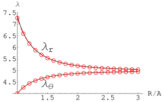
(a) The parameter values are $vN=10^{-4}$ and $\chi=0.2$ ($\alpha=4.95934$), $B=3A$ and $\lambda_{0}=4$ (correspondingly $\lambda_{0}^{\ast}\approx-1$).

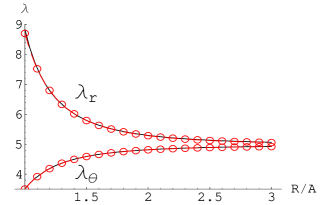
(b) The parameter values are $vN=10^{-4}$ and $\chi=0.2$ ($\alpha=4.95934$), $B=3A$ and $\lambda_{0}=3.5$ (correspondingly $\lambda_{0}^{\ast}\approx-1.5$).

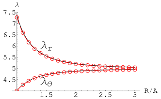
(c) The parameter values are $vN=10^{-4}\times 2/3$ and $\chi=0.3$ ($\alpha=4.95934$), $B=3A$ and $\lambda_{0}=4$ (correspondingly $\lambda_{0}^{\ast}\approx-1$).

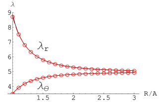
(d) The parameter values are $vN=10^{-4}\times 2/3$ and $\chi=0.3$ ($\alpha=4.95934$), $B=3A$ and $\lambda_{0}=3.5$ (correspondingly $\lambda_{0}^{\ast}\approx-1.5$).

Figure 1: Distributions of the stretches (lines -o- are the analytical solutions and black solid lines are the numerical solutions).

For the chosen geometric parameter in Figure 1, we have $a=0.5$. Although the value of $\alpha$ is not very large, it can be seen that the analytical solution agrees with the numerical one very well. Actually, the maximum relative errors of $(\lambda_{\theta},\lambda_{r})$ are only about $(0.2\%,1\%)$,$(0.2\%,1.5\%)$,$(0.3\%,1.3\%)$ and $(0.2\%,1.7\%)$ respectively for the four figures.

We also point out that $(vN,\chi)$ have different values in Figures $(a,b)$ and Figures $(c,d)$, but the $\alpha$ value is the same in all cases. So, the analytical solutions in Figures $(a,c)$ and Figures $(b,d)$ are the same respectively. The agreement between the analytical solutions and numerical ones show that the deformation is mainly determined by the single hydrogel deformation constant $\alpha$, although the free-energy function contains two material constants $(vN,\chi)$.

Normally when the outer boundary condition $s_{r}(B)=0$ is used, the stress $s_{\theta}$ is not 0 but an $O(1)$ quantity (see $(\ref{eq26})_{3}$). Now, we consider the case that $s_{\theta}(B)=0$ instead of $s_{r}(B)=0$. In this case, the boundary condition $(\ref{eq14})$ is replaced by

$$u(1)-\frac{1}{u^{3}(1)\left[u(1)+(a+1)u^{\prime}(1)\right]}-\alpha^{-2}\frac{1}{u(1)}+O(\alpha^{-3})=0.$$ (30)

One can proceed to construct the perturbation expansion solution as before. The solution expression is still given by $(\ref{eq24})$ but now the expressions for the constants are replaced by

$$c_{1}=\frac{5a^{3}(1+a)^{3}\lambda_{0}^{\ast}}{5(1+a)^{3}-2a^{3}},\quad c_{2}=\frac{-2a^{3}\lambda_{0}^{\ast}}{5(1+a)^{3}-2a^{3}},$$ (31)

$$d_{1}=\frac{a^{3}(1+a)^{3}(5M_{1}-M_{2})}{5(1+a)^{3}-2a^{3}},\quad d_{2}=\frac{(1+a)^{3}M_{2}-2a^{3}M_{1}}{5(1+a)^{3}-2a^{3}},$$ (32)

where $M_{1}$ is given by $(\ref{eq23})_{1}$ and

$$M_{2}=1+\frac{10c_{1}^{2}}{3(1+a)^{6}}+\frac{5c_{1}c_{2}}{(1+a)^{3}}+10c_{2}^{2}.$$ (33)

Simple analytical formulas can also be obtained for the stretches and stresses at the inner and outer surfaces, and here we omit the details.

5 Analytical Solution for a General Inhomogeneous Deformation

In the previous section, we have assumed that at the inner surface the given stretch $\lambda_{0}$ satisfies the constraint $|\lambda_{0}-\alpha|\ll\alpha$. In that case, basically the governing equation can be linearized around $r=\alpha R$ so the analytical solution can be obtained by solving linear differential equations. Now, we shall proceed to construct the solution without the above constraint. Instead, it is supposed that the stretch $\lambda_{0}$ at $R=A$ is far away from $\alpha$ such that $\lambda_{0}$ is an $O(1)$ quantity. For this problem, one cannot avoid to deal with some nonlinear second-order variable-coefficient differential equation(s).

As mentioned before, for a hydrogel the material constant $vN$ is small, so we always take $\alpha$ as a large parameter or $\alpha^{-1}$ as a small parameter. In general, one cannot solve a nonlinear differential equation analytically. However, if a small parameter is present in the equation, sometimes one can use singular perturbation methods to construct asymptotic solutions. But, for those methods to work, usually the equation should become degenerate as the small parameter tends to zero, say, it becomes a linear equation or it becomes a first-order equation instead of the original second-order equation. For the present problem governed by $(\ref{eq13})$, we see that as $\alpha^{-1}$ tends to zero the leading-order equation is still a complicated nonlinear second-order variable-coefficient equation. This shows that the existing singular perturbation methods do not work for this equation. Here, we introduce a novel methodology, which is an extension of the method of matched asymptotics, to construct the analytical solution.

We consider the case that the thickness of the shell is relatively large (an explicit restriction will be provided later on). We first make some observations on the solution structure. For a thick shell, the boundary condition at the inner surface should not influence a region some distance away from it (we assume that the St. Venant’s principle applies). So, there is a region containing the outer boundary point in which the deformation is near a free-swelling one as the stress-free condition can then be satisfied automatically (to the leading order). We call this region to be the outer region. When $|\lambda_{0}-\alpha|\ll\alpha$, we see from Figure 1 that in a region near the inner surface the stretches change rapidly. It is reasonable to expect that when $\lambda_{0}=O(1)$ the stretches also change rapidly in this region. In other words, there is a boundary layer region near the inner surface, and we call this region to be the inner region. This kind of structure can also be seen from the numerical solutions obtained in Zhao et al..[27] In the standard technique of matched asymptotics[17] only an inner region and an outer region exist and the equation in the latter region is one-order less than that in the former region. By solving the equations in both regions separately and then matching the two solutions together to determine the integration constants, the asymptotic solution can be obtained. However, for the present problem, the leading-order equation in the outer region, which can be obtained by setting $\alpha^{-1}=0$ in $(\ref{eq13})$, is still a second-order differential equation, so one cannot simply match the solutions in the inner region and outer region directly. To connect them there should be a third region in between, which will be called a transition region. We shall use this transition region to connect the outer and inner regions. However, a major difficulty arises: In this region one has to deal with the full nonlinear second-order variable-coefficient differential equation, which is not solvable analytically! We shall overcome this difficulty by using a series expansion for the solution in this region whose interval should be small. The details are described below.

(a) Solution in the outer region

First we consider the outer solution. The governing equation is still $(\ref{eq13})$, and the boundary condition $(\ref{eq14})$ can still be used in the outer region. As mentioned before, it is expected that in this region the deformation is near a free-swelling one. Therefore, we seek a perturbation expansion solution of the form

$$u(s)=1+\alpha^{-2}u_{1}(s)+\cdots.$$ (34)

Here, the second-order term is set to be $O(\alpha^{-2})$, to be consistent with the governing equation $(\ref{eq13})$ and boundary condition $(\ref{eq14})$. We substitute this expansion into $(\ref{eq13})$ and $(\ref{eq14})$. At $O(1)$, they are automatically satisfied. At $O(\alpha^{-2})$, we find that $u_{1}(s)$ satisfies $(\ref{eq17})$, and the solution expression is

$$u_{1}(s)=C_{3}(s+a)^{-3}+C_{2},$$ (35)

where $C_{2}$ and $C_{3}$ are two integration constants. By further using $(\ref{eq14})$, we obtain

$$u_{1}(s)=\frac{(5C_{2}-1)(1+a)^{3}}{4(s+a)^{3}}+C_{2}.$$ (36)

To sum up, the outer solution is given by

$$\tilde{r}_{out}(s):=\frac{r_{out}(s)}{A}=\alpha\frac{s+a}{a}+\alpha^{-1}\left[\frac{(5C_{2}-1)(1+a)^{3}}{4a(s+a)^{2}}+\frac{C_{2}(s+a)}{a}\right],$$ (37)

where $C_{2}$ is to be determined.

(b) Solution in the inner region

Next we consider the inner region (i.e. boundary layer), we should examine the full equation $(\ref{eq13})$. To simplify the equation we introduce the variable $\bar{r}$ by

$$\frac{r}{A}=\tilde{r}=\alpha\bar{r}(s)\quad\Rightarrow\quad u(s)=\frac{a\bar{r}(s)}{s+a}.$$ (38)

Then the equation (12) becomes

$$\left[a^{2}+\frac{2(s+a)^{2}}{a^{3}\bar{r}^{2}(s)[\bar{r}^{\prime}(s)]^{3}}\right]\bar{r}^{\prime\prime}(s)+\frac{2a^{2}\bar{r}^{\prime}(s)}{(s+a)}-\frac{2a^{2}\bar{r}(s)}{(s+a)^{2}}-\frac{4(s+a)}{a^{3}\bar{r}^{2}(s)[\bar{r}^{\prime}(s)]^{2}}$$ (39)

$$+\frac{4(s+a)^{2}}{a^{3}\bar{r}^{3}(s)\bar{r}^{\prime}(s)}+\alpha^{-2}\left[\frac{(a+s)\bar{r}^{\prime\prime}(s)-2\bar{r}^{\prime}(s)}{(a+s)[\bar{r}^{\prime}(s)]^{2}}+\frac{2}{\bar{r}(s)}\right]=0.$$

Suppose that in this region the maximum value $\bar{r}_{max}=O(\alpha^{-k})$ ($k$ is to be determined) and we write $\bar{r}=\alpha^{-k}\hat{r}$. We note that the value of $\bar{r}$ at the inner surface is $O(\alpha^{-1})$ due to the condition $\tilde{r}=\lambda_{0}=O(1)$. $\bar{r}_{max}$ should be much larger than this value due to the rapid increase of $\bar{r}$ in the boundary layer region. Thus a restriction is $k<1$. To reflect the rapid change of $\bar{r}$ in the boundary layer, we introduce the stretching coordinate $X=s/(a\epsilon)$, where $a\epsilon$, the parameter characterizing the thickness of the boundary layer, is to be determined. Making this change of variables to equation $(\ref{eq45})$, according to the Van Dyke’s principle of least degeneracy,[6] we find $\epsilon=\alpha^{-5k/3}$. Since $\epsilon$ should be small, we need $k>0$. And, the equation becomes

$$\left[1+\frac{2}{\hat{r}^{2}\hat{r}_{{}_{X}}^{3}}\right]\hat{r}_{{}_{XX}}+\frac{4}{\hat{r}^{3}\hat{r}_{{}_{X}}}+O(\epsilon)+O(\epsilon^{2})+O(\epsilon^{2}\alpha^{2k-2})=0,$$ (40)

where we denote $\hat{r}_{{}_{X}}=\frac{d\hat{r}}{dX}$ to distinguish from $\hat{r}^{\prime}(s)$. Since $0<k<1$, $O(\alpha^{2k-2})$ is small. If one uses the Van Dyke’s principle of least degeneracy for the $O(\epsilon^{3})$ equation, it is required that $O(\epsilon^{2}\alpha^{2k-2})=O(\epsilon^{3})$, i.e., $k=6/11$. Then, the boundary layer thickness parameter $a\epsilon=a\alpha^{-10/11}$, which needs to be small, say, $a\epsilon<0.15$. Thus, a restriction is $a<0.15\alpha^{10/11}$.

Multiplying both sides by $\hat{r}_{{}_{X}}$ and integrating once, we obtain (to the leading order)

$$\hat{r}_{{}_{X}}^{2}-\frac{4}{\hat{r}^{2}\hat{r}_{{}_{X}}}=C_{1},$$ (41)

where $C_{1}$ is the integration constant. This is a first-order differential equation. With the boundary condition $\tilde{r}(0)=\lambda_{0}$, theoretically there is only one constant $C_{1}$ to be determined. Actually, the solution $\hat{r}_{in}$ of the above equation can be represented by

$$X=\int_{\hat{\lambda}_{0}}^{\hat{r}_{in}}\frac{dy}{f(y;C_{1})},$$ (42)

where $\hat{\lambda}_{0}:=\lambda_{0}\alpha^{-5/11}$ is a known constant and $f$ is the root of the cubic algebraic equation

$$F(f)=f^{3}-C_{1}f-\frac{4}{y^{2}}=0.$$ (43)

For the present problem we require $f=\hat{r}_{{}_{X}}>0$ with $y=\hat{r}>0$. It is easy to show that equation $(\ref{eq50})$ has one and only one positive root, which is given by

$$f(y;C_{1})=\begin{cases}-\frac{C_{1}y^{2/3}}{3\sqrt[3]{2}\left[\sqrt{1-C_{1}^{3}y^{4}/108}-1\right]^{1/3}}-\frac{\sqrt[3]{2}\left[\sqrt{1-C_{1}^{3}y^{4}/108}-1\right]^{1/3}}{y^{2/3}},&C_{1}<0,\\ \sqrt[3]{4}/y^{2/3},&C_{1}=0,\\ \frac{C_{1}y^{2/3}}{3\sqrt[3]{2}\left[1-\sqrt{1-C_{1}^{3}y^{4}/108}\right]^{1/3}}+\frac{\sqrt[3]{2}\left[1-\sqrt{1-C_{1}^{3}y^{4}/108}\right]^{1/3}}{y^{2/3}},&C_{1}>0.\\ \end{cases}$$ (44)

In summary, the inner solution is provided by $(\ref{eq49})$ and $(\ref{eq51})$ with one constant $C_{1}$ to be determined.

(c)Solution in the transition region

Now, we consider the transition region, which is used to connect both the inner and outer regions. Since $\tilde{r}$ (or $\lambda_{\theta}$) is $O(\alpha^{5/11})$ and $O(\alpha)$ respectively for the inner and outer regions, such a transition region is needed to get the whole solution in the whole interval. The independent variable $s$ is in the interval $[0,1]$, and we schematically represent the three regions in Figure 2. In this figure, the transition region is represented by $[s_{0}-\Delta,s_{0}+\Delta]$, where $s_{0}$ and $\Delta$ are to be determined.

Figure 2: The geometric representation of the three regions.

In this region, we should use the full equation $(\ref{eq45})$, and we have (to the leading order)

$$\left[a^{2}+\frac{2(s+a)^{2}}{a^{3}\bar{r}^{2}(s)[\bar{r}^{\prime}(s)]^{3}}\right]\bar{r}^{\prime\prime}(s)+\frac{2a^{2}\bar{r}^{\prime}(s)}{(s+a)}-\frac{2a^{2}\bar{r}(s)}{(s+a)^{2}}$$ (45)

$$-\frac{4(s+a)}{a^{3}\bar{r}^{2}(s)[\bar{r}^{\prime}(s)]^{2}}+\frac{4(s+a)^{2}}{a^{3}\bar{r}^{3}(s)\bar{r}^{\prime}(s)}=0.$$

This is a nonlinear second-order variable-coefficient differential equation, which appears to be not solvable analytically! To proceed further, we observe the following: The whole interval for $s$ is $[0,1]$, which is divided into three regions: outer region, transition region and inner region. Since usually the outer region is large in a singular perturbation problem (this is also evident from the numerical solutions in Zhao et al.[27]), the transition region should only occupy a small subinterval of $[0,1]$. Thus, for $s$ in the small subinterval $[s_{0}-\Delta,s_{0}+\Delta]$ the solution of the above nonlinear equation can be expanded as a series (as long as $\bar{r}(s)$ is sufficiently smooth):

$$\bar{r}_{tran}(s)=r_{0}+r_{1}(s-s_{0})+r_{2}(s-s_{0})^{2}+r_{3}(s-s_{0})^{3}+\cdots,$$ (46)

where $r_{i}(i=0,1,2,3)$ together with $s_{0}$ need to be determined. Substituting this expansion into equation $(\ref{eq52})$, the left hand side becomes a series of $(s-s_{0})$. All the coefficients of $(s-s_{0})^{n}(n=0,1,2,3,\cdots)$ should be zero. From the coefficients of $(s-s_{0})^{0}$ and $(s-s_{0})$, we can obtain two algebraic relations among the undetermined coefficients, which are represented as

$$f_{1}(s_{0},r_{0},r_{1},r_{2})=0,$$ (47)

$$f_{2}(s_{0},r_{0},r_{1},r_{2},r_{3})=0,$$

where the lengthy expressions of $f_{1}$ and $f_{2}$ are omitted. To have enough relations for the determination of all constants, we need to relate the transition solution to the outer and inner solutions.

(d) Determination of the constants through connection conditions

We have obtained the solution expressions in the outer region, inner region and transition region (see equations $(\ref{eq43}),(\ref{eq49})$ and $(\ref{eq53})$). Each of the outer and inner solutions contains one constant and the transition solution contains five constants. The subinterval $[s_{0}-\Delta,s_{0}+\Delta]$ also needs to be found, so we have another constant $\Delta$ to determine. Besides equations $(\ref{eq54})_{1,2}$, we need another six relations for the eight constants $C_{1},C_{2},s_{0},\Delta,r_{i}(i=0,1,2,3)$, which can be obtained by requiring $r,r^{\prime},r^{\prime\prime}$ are all continuous at $s_{0}-\Delta$ and $s_{0}+\Delta$, i.e.

$$r_{in}(s)=r_{tran}(s),\ r_{in}^{\prime}(s)=r_{tran}^{\prime}(s),\ r_{in}^{\prime\prime}(s)=r_{tran}^{\prime\prime}(s),\quad\ {\rm at}\ s=s_{0}-\Delta,$$ (48)

$$r_{tran}(s)=r_{out}(s),\ r_{tran}^{\prime}(s)=r_{out}^{\prime}(s),\ r_{tran}^{\prime\prime}(s)=r_{out}^{\prime\prime}(s),\ {\rm at}\ s=s_{0}+\Delta.$$

To reduce the above six relations into two relations, by using the solution expression $(\ref{eq53})$ we rewrite them as

$$r_{0}-r_{1}\Delta+r_{2}\Delta^{2}-r_{3}\Delta^{3}+O(\Delta^{4})=\tilde{r}_{in}(s_{0}-\Delta;C_{1})/\alpha,$$ (49)

$$r_{1}-2r_{2}\Delta+3r_{3}\Delta^{2}+O(\Delta^{3})=\tilde{r}^{\prime}_{in}(s_{0}-\Delta;C_{1})/\alpha,$$

$$2r_{2}-6r_{3}\Delta+O(\Delta^{2})=\tilde{r}^{\prime\prime}_{in}(s_{0}-\Delta;C_{1})/\alpha,$$

$$r_{0}+r_{1}\Delta+r_{2}\Delta^{2}+r_{3}\Delta^{3}+O(\Delta^{4})=\tilde{r}_{out}(s_{0}+\Delta;C_{2})/\alpha,$$

$$r_{1}+2r_{2}\Delta+3r_{3}\Delta^{2}+O(\Delta^{3})=\tilde{r}^{\prime}_{out}(s_{0}+\Delta;C_{2})/\alpha,$$

$$2r_{2}+6r_{3}\Delta+O(\Delta^{2})=\tilde{r}^{\prime\prime}_{out}(s_{0}+\Delta;C_{2})/\alpha.$$

By some simple manipulations, $r_{j}(j=0,1,2,3)$ can be eliminated, and as a result two equations for the four constants $s_{0},\Delta,C_{1},C_{2}$ are obtained

$$-3\tilde{r}_{in}+3\tilde{r}_{out}+2\Delta\left(-3\tilde{r}_{out}^{\prime}+\Delta\tilde{r}_{in}^{\prime\prime}+2\Delta\tilde{r}_{out}^{\prime\prime}\right)=0,$$ (50)

$$-3\tilde{r}_{in}+3\tilde{r}_{out}-2\Delta\left(3\tilde{r}_{in}^{\prime}+2\Delta\tilde{r}_{in}^{\prime\prime}+\Delta\tilde{r}_{out}^{\prime\prime}\right)=0.$$

where the subscripts “in” and “out” represent the value at $s_{0}-\Delta$ and $s_{0}-\Delta$ respectively. Another two equations for $s_{0},\Delta,C_{1},C_{2}$ are provided by $(\ref{eq54})_{1,2}$. By the Newton’s method, these constants can be easily found.

To get the solution curve, we take the parameters $vN=10^{-4}$ and $\chi=0.2$, which yields that $\alpha\approx 5$. For the geometrical parameter we choose two different values $B=3A$ and $4A$ (i.e., $a=0.5$ and $1/3$). The stretch at the inner surface is chosen to be $\lambda_{0}=1.077$ (which is an $O(1)$ quantity). For such parameters, by solving the system of 4 algebraic equations mentioned above, we find

$$a=0.5:\ s_{0}=0.2127,\Delta=0.06265,C_{1}=-0.008259,C_{2}=-0.2449,$$ (51)

$$a=1/3:\ s_{0}=0.1670,\Delta=0.04386,C_{1}=0.0008190,C_{2}=0.01042.$$

For such parameters, we have $\epsilon=\alpha^{-10/11}=0.2332$. The parameter $a\epsilon$, a measure of the magnitude of the boundary layer thickness has the values about $0.12$ and $0.08$ for $a=0.5$ and $1/3$ respectively, which are consistent with the values of $s_{0}-\Delta$ (0.15 and 0.12). The subintervals of the transition region $[0.150,0.275]$ and $[0.123,0.211]$ (for $a=0.5$ and $a=1/3$ respectively) are indeed small, as observed before. For such small intervals, the series solution $(\ref{eq53})$ should be very accurate.

Finally we compare our analytical solution with the numerical one obtained by a shooting method. The solution curves obtained by two methods for the above chosen parameters are plotted in Figure 3.

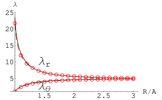
(a) The parameter values are $vN=10^{-4}$ and $\chi=0.2$ ($\alpha=4.95934$), $B=3A$ and $\lambda_{0}=1.077$.

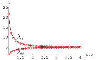
(b) The parameter values are $vN=10^{-4}$ and $\chi=0.2$ ($\alpha=4.95934$), $B=4A$ and $\lambda_{0}=1.077$.

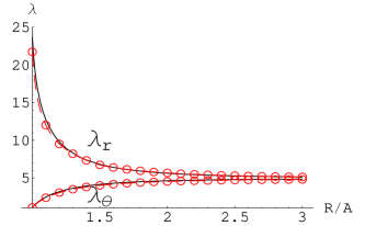
(c) The parameter values are $vN=10^{-4}\times 2/3$ and $\chi=0.3$ ($\alpha=4.95934$), $B=3A$ and $\lambda_{0}=1.077$.

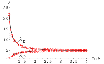
(d) The parameter values are $vN=10^{-4}\times 2/3$ and $\chi=0.3$ ($\alpha=4.95934$), $B=4A$ and $\lambda_{0}=1.077$.

Figure 3: Distributions of the stretches (lines -o- are the analytical solutions and black solid lines are the numerical solutions).

It can be seen that the analytical solution agrees well with the numerical solution. Actually, the maximum relative errors of $(\lambda_{\theta},\lambda_{r})$ are about $(2.7\%,7.7\%)$, $(2.9\%,8.0\%)$, $(2.8\%,8.1\%)$, $(3.0\%,8.4\%)$ respectively for the four figures. Keeping in mind that the obtained analytical solution is only valid up to $O(1)$ and the $O(\epsilon)$ ($=O(\alpha^{-10/11})$) terms are omitted, it produces reasonable good results already.

In Figures 3$(a,b)$ and Figures 3$(c,d)$, the values of $(vN,\chi)$ are different. However, in all cases the $\alpha$ value is same. Since the analytical solution depends only on the $\alpha$ value, the analytical curves in Figures $3(a,c)$ and Figures $3(b,d)$ are the same respectively. The agreement between the analytical and numerical solutions once again shows that the deformation is mainly determined by the single material constant – the hydrogel deformation constant $\alpha$.

Now we shall give a more explicit expression than equation $(\ref{eq49})$ for the inner solution. As it can be seen from $(\ref{eq60})$ that $C_{1}$ is small, we seek a perturbation expansion solution of equation $(\ref{eq48})$ of the form

$$\hat{r}_{in}=r^{*}_{0}(X)+C_{1}r^{*}_{1}(X)+\cdots.$$ (52)

Substituting the above expansion into equation $(\ref{eq48})$ and using the boundary condition $\hat{r}(0)=\hat{\lambda}_{0}$, we obtain

$$\hat{r}_{in}(s)= \left(\frac{5\sqrt[3]{4}}{3}X+\hat{\lambda}_{0}^{5/3}\right)^{3/5}+$$ (53)

$$\frac{C_{1}}{{18\sqrt[3]{2}}}\left[\left(\frac{5\sqrt[3]{4}}{3}X+\hat{\lambda}_{0}^{5/3}\right)^{7/5}-\hat{\lambda}_{0}^{3}\left(\frac{5\sqrt[3]{4}}{3}X+\hat{\lambda}_{0}^{5/3}\right)^{-2/5}\right],$$

where $X=s/(a\epsilon)=\alpha^{10/11}s/a$. Then $\tilde{r}_{in}$ can be immediately recovered by $\tilde{r}_{in}(s)=\alpha^{5/11}\hat{r}_{in}(s)$. In Figure 4, we plot the solution curves of $(\ref{eq49})$ and $(\ref{eq62})$. It can be seen that the difference is very small. This supports the validity of the more explicit expression $(\ref{eq62})$.

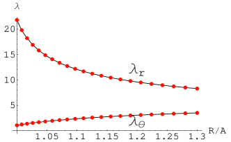
(a) The parameter values are $vN=10^{-4}$ and $\chi=0.2$, $B=3A$ and $\lambda_{0}=1.077$.

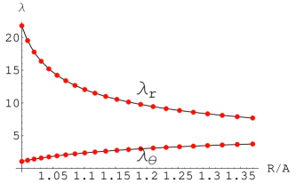
(b) The parameter values are $vN=10^{-4}$ and $\chi=0.2$, $B=4A$ and $\lambda_{0}=1.077$.

Figure 4: Comparison of the two inner solutions (dots are the solution (42) and solid lines are the explicit solution (53)).

Since we have obtained the analytical solution, some simple approximate analytical formulas for important physical quantities can be deduced. As in the previous section, we consider the stresses and stretches at the inner and outer surfaces. At the inner surface $R=A$, we have

$$\begin{array}[]{ll}\displaystyle\lambda_{\theta}=\lambda_{0},&\displaystyle\lambda_{r}=\frac{\sqrt[3]{4}\alpha^{5/3}}{\lambda_{0}^{2/3}}+\frac{C_{1}\alpha^{35/33}\lambda_{0}^{2/3}}{3\sqrt[3]{4}},\\ \displaystyle\frac{s_{\theta}}{NkT}=-\frac{\alpha^{10/3}}{\sqrt[3]{4}\lambda_{0}^{7/3}}+\frac{C_{1}\alpha^{30/11}}{12\lambda_{0}},&\displaystyle\frac{s_{r}}{NkT}=\frac{3\alpha^{5/3}}{2\sqrt[3]{2}\lambda_{0}^{2/3}}+\frac{C_{1}\alpha^{35/33}\lambda_{0}^{2/3}}{2\sqrt[3]{4}}.\end{array}$$ (54)

We can see that radial stretch $\lambda_{r}$ and radial stress $s_{r}/NkT$ are $O(\alpha^{5/3})$ quantities, while the circumferential stress $s_{\theta}/NkT$ is much larger, an $O(\alpha^{10/3})$ quantity. What is more, if $C_{1}$-terms are neglected ($C_{1}$ is small), all the stresses and stretches at the inner surface are unaffected by the geometric parameter $a$, the ratio of the inner radius to the thickness. It should be pointed out that, although $C_{1}$ is small, its value depends on $a$. In the above cases, the $C_{1}$-terms in $(\ref{eq63})$ only have a minor influence (less than $0.3\%$, compared with the first terms).

At the outer surface $R=B$, we have

$$\begin{array}[]{ll}\displaystyle\lambda_{\theta}=\alpha-\alpha^{-1}\frac{1-9C_{2}}{4},&\displaystyle\lambda_{r}=\alpha+\alpha^{-1}\frac{1-3C_{2}}{2},\\ \displaystyle\frac{s_{\theta}}{NkT}=\frac{-3(1-5C_{2})}{2}\alpha^{-1},&\displaystyle\frac{s_{r}}{NkT}=0.\end{array}$$ (55)

Comparing with equation $(\ref{eq10})$, we see that the stretch $\lambda_{\theta}$ is close to but a little smaller than $\lambda_{free}$ while the stretch $\lambda_{r}$ is close to but a little larger than $\lambda_{free}$. The circumferential stress $s_{\theta}/(NkT)$ is of $O(\alpha^{-1})$, which implies that a very small stress needs to be applied to maintain this spherically symmetric deformation.

If we impose the boundary condition $s_{\theta}(B)=0$ instead of $s_{r}(B)=0$, the analytical solution can be constructed by the same procedure described above. Actually, in this case only the expression of the outer solution changes to

$$\tilde{r}_{out}(s)=\alpha\frac{s+a}{a}+\alpha^{-1}\left[\frac{(1-5C_{2})(1+a)^{3}}{2a(s+a)^{2}}+\frac{C_{2}(s+a)}{a}\right].$$ (56)

The expressions of the inner and transition solutions and the connection conditions are all the same. Also, the stresses and stretches at the inner surface are still given by equation $(\ref{eq63})$. And, at the outer surface we have

$$\begin{array}[]{ll}\displaystyle\lambda_{\theta}=\alpha+\alpha^{-1}\frac{1-3C_{2}}{2},&\displaystyle\lambda_{r}=\alpha+\alpha^{-1}(6C_{2}-1)\\ \displaystyle\frac{s_{\theta}}{NkT}=0,&\displaystyle\frac{s_{r}}{NkT}=3(5C_{2}-1)\alpha^{-1}.\end{array}$$ (57)

We see that in this case an $O(\alpha^{-1})$ tensile stress needs to be applied at the outer surface to maintain this deformation.

6 Conclusions

We study analytically three cases of hydrogel swelling for a core-shell structure, i.e. a free-swelling deformation, a near-free swelling deformation and a general inhomogeneous deformation. The hydrogel deformation constant $\alpha$, which is a combination of the two material parameters $vN$ and $\chi$, is identified, and it is found that this single material parameter plays a dominant role for the deformations in all three cases. For the free swelling deformation, a simple formula for the stretch $\lambda_{free}$ is obtained in terms of $\alpha$ up to $O(\alpha^{-1})$. For the near-free swelling one, we obtain the analytic solution for the whole region. Some analytical formulas for the stresses and stretches at the inner and outer surfaces are given, and it turns out they depend linearly on the value $\lambda_{0}-\alpha$ (where $\lambda_{0}$ is the given stretch at the inner surface). In this case, for a thick shell (the ratio $a$ of the inner radius to the shell thickness is small), the geometrical parameter $a$ has little effect. When the shell is thin it is not stress-free in the circumferential direction at the outer surface, which indicates the boundary conditions $s_{r}(B)=0$ and $s_{\theta}(B)=0$ are not equivalent. For the general inhomogeneous one, we treat it as a boundary layer problem. An extended method of matched asymptotics is introduced to solve this problem. More specifically a transition region is introduced to connect the inner region and outer region. Further, we seek a series solution in the transition region and impose proper connections with the inner and outer solutions. Then, theoretically the problem is reduced to solve a system of 4 algebra equations. Analytical formulas for the radial and hoop stresses and stretches at the inner surface are obtained. It is found that both the radial and hoop stresses are very large and the former is an $O(\alpha^{5/3})$ quantity while the latter is an $O(\alpha^{10/3})$ quantity. Also, these quantities are independent of the geometric parameter $a$ (to the leading order). Numerical comparisons are also performed, and the results are in good agreement with the analytical ones.

References

• [1] M. Ballauff and Y. Lu, β€œSmart” nanoparticles: preparation, characterization and applications, Polymer 48 (2007) 1815–1823.
• [2] A. Biffis and L. Minati, Efficient aerobic oxidation of alcohols in water catalysed by microgel-stabilised metal nanoclusters, Journal of Catalysis 236 (2005) 405–409.
• [3] A. Biffis, N. Orlandi and B. Corain, Microgel-Stabilized metal Nanoclusters: Size Control by Microgel Nanomorphology, Advanced Materials 15 (2003) 1551–1555.
• [4] M. A. Biot, General theory of three-dimensional consolidation, Journal of Applied Physics 12 (1941) 155–164.
• [5] M. A. Biot, Nonlinear and semilinear Rheology of Porous Solids, Journal of Geophysical Research 78 (1973) 4924–4937.
• [6] A. W. Bush, Perturbation methods for engineers and scientists (CRC Press, 1992).
• [7] J. J. Crassous and M. Ballauff, Imaging the Volume Transition in Thermosensitive Core-Shell Particles by Cryo-Transmission Electron Microscopy, American Chemical Society 22 (2006) 6.
• [8] M. Das, S. Mardyani, W. C. W. Chan and E. Kumacheva, Biofunctionalized pH-Responsive Microgels for Cancer Cell Targeting: Rational Design, Advanced Materials 18 (2006) 80–83.
• [9] F. Dolbow, E. Fried and H. Ji, Chemically induced swelling of hydrogels, Journal of the Mechanics and Physics of Solids 52 (2004) 51–84.
• [10] F. Dolbow, E. Fried and H. Ji, A numerical strategy for investigating the kinetic response of stimulus-responsive hydrogels, Computer Methods in Applied Mechanics and Engineering 194 (2005) 4447–4480.
• [11] C. J. Durning and K. N. Morman, Nonlinear swelling of polymer gels, Journal of Chemical Physics 98 (1993) 4275–4293.
• [12] J. D. Ferry, Viscoelastic Properties of Polymers (Wiley, 1980).
• [13] P. J. Flory, Principles of polymer chemistry (Cornell University Press, 1953).
• [14] P. J. Flory and J. Rehner, Statistical Mechanics of Cross-Linked Polymer Networks II. Swelling, The Journal of Chemical Physics 11 (1943) 521–526.
• [15] J. W. Gibbs, On the equilibrium of Heterogeneous Substances, Transactions of the connecticut Academy of Arts and Sciences 3 (1878) 108–248.
• [16] J. Guo, W. Yang, Y. Deng, C. Wang and S. Fu, Organic-dye-coupted magnetic nanoparticles encaged inside thermoresponsive PNIPAM microcapsutes, small 1 (2005) 737–743.
• [17] M. H. Holmes, Introduction to perturbation methods (Springer-Verlag, 1995).
• [18] W. Hong, Z. Liu and Z. Suo, Inhomogeneous swelling of a gel in equilibrium with a solvent and mechanical load, International Journal of Solids and Structures 46 (2009) 3282–3289.
• [19] W. Hong, X. Zhao and J. Zhou and Z. Suo, A theory of coupled diffusion and large deformation in polymeric gels, Journal of the Mechanics and Physics of Solids 56 (2008) 1779–1793.
• [20] H. Kawaguchi and K. Fujimoto, Smart latexes for bioseparation, Bioseparation 7 (1999) 253–258.
• [21] J.-H. Kim and T. R. Lee, Discrete Thermally Responsive Hydrogel-Coated Gold Nanoparticles for Use as Drug-Delivery Vehicles, Drug Development Research 67 (2006) 61–69.
• [22] S. Nayak, H. Lee, J. Chmielewski and L. A. Lyon, Folate-Mediated Cell Targeting and Cytotoxicity Using Thermoresponsive Microgels, Journal of The American Chemical Society 126 (2004) 10258–10259.
• [23] T. J. Pence and H. Tsai, Swelling-induced microchannel formation in nonlinear elasticity, IMA Journal of Applied Mathematics 70 (2005) 173–189.
• [24] T. J. Pence and H. Tsai, On the cavitation of a swollen compressible sphere in finite elasticity, International Journal of Non-Linear Mechanics 40 (2005) 307–321.
• [25] T. J. Pence and H. Tsai, Bulk Cavitation and the Possibility of Localized Interface Deformation due to Surface Layer Swelling, Journal of Elasticity 87 (2007) 161–185.
• [26] H. Tsai, T. J. Pence and E. Kirkinis, Swelling Induced Finite Strain Flexure in a Rectangular Block of an Isotropic Elastic Material, Journal of Elasticity 75 (2004) 69–89.
• [27] X. Zhao and W. Hong and Z. Suo, Inhomogeneous and anisotropic equilibrium state of a swollen hydrogen containing a hard core, Applied Physics Letters 92 (2008) 051904.