Distributed Estimation via Iterative Projections with Application to Power Network Monitoring

Abstract

This work presents a distributed method for control centers to monitor the operating condition of a power network, i.e., to estimate the network state, and to ultimately determine the occurrence of threatening situations. State estimation has been recognized to be a fundamental task for network control centers to ensure correct and safe functionalities of power grids. We consider (static) state estimation problems, in which the state vector consists of the voltage magnitude and angle at all network buses. We consider the state to be linearly related to network measurements, which include power flows, current injections, and voltages phasors at some buses. We admit the presence of several cooperating control centers, and we design two distributed methods for them to compute the minimum variance estimate of the state given the network measurements. The two distributed methods rely on different modes of cooperation among control centers: in the first method an incremental mode of cooperation is used, whereas, in the second method, a diffusive interaction is implemented. Our procedures, which require each control center to know only the measurements and structure of a subpart of the whole network, are computationally efficient and scalable with respect to the network dimension, provided that the number of control centers also increases with the network cardinality. Additionally, a finite-memory approximation of our diffusive algorithm is proposed, and its accuracy is characterized. Finally, our estimation methods are exploited to develop a distributed algorithm to detect corrupted data among the network measurements.

, ,

1 Introduction

Large-scale complex systems, such as, for instance, the electrical power grid and the telecommunication system, are receiving increasing attention from researchers in different fields. The wide spatial distribution and the high dimensionality of these systems preclude the use of centralized solutions to tackle classical estimation, control, and fault detection problems, and they require, instead, the development of new decentralized techniques. One possibility to overcome these issues is to geographically deploy some monitors in the network, each one responsible for a different subpart of the whole system. Local estimation and control schemes can successively be used, together with an information exchange mechanism to recover the performance of a centralized scheme.

1.1 Control centers, state estimation and cyber security in power networks

Power systems are operated by system operators from the area control center. The main goal of the system operator is to maintain the network in a secure operating condition, in which all the loads are supplied power by the generators without violating the operational limits on the transmission lines. In order to accomplish this goal, at a given point in time, the network model and the phasor voltages at every system bus need to be determined, and preventive actions have to be taken if the system is found in an insecure state. For the determination of the operating state, remote terminal units and measuring devices are deployed in the network to gather measurements. These devices are then connected via a local area network to a SCADA (Supervisory Control and Data Acquisition) terminal, which supports the communication of the collected measurements to a control center. At the control center, the measurement data is used for control and optimization functions, such as contingency analysis, automatic generation control, load forecasting, optimal power flow computation, and reactive power dispatch [1]. A diagram representing the interconnections between remote terminal units and the control center is reported in Fig. 1.

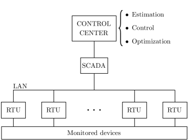
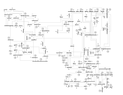
Figure 1: In Fig. 1, remote terminal units (RTU) transmit their measurements to a SCADA terminal via a LAN network. The data is then sent to a Control Center to implement network estimation, control, and optimization procedures. Fig. 1 shows the diagram of the IEEE 118 bus system (courtesy of the IIT Power Group). The network has 118 buses, 186 branches, 99 loads, and 54 generators.

Various sources of uncertainties, e.g., measurement and communication noise, lead to inaccuracies in the received data, which may affect the performance of the control and optimization algorithms, and, ultimately, the stability of the power plant. This concern was first recognized and addressed in [27, 28, 29] by introducing the idea of (static) state estimation in power systems.

Power network state estimators are broadly used to obtain an optimal estimate from redundant noisy measurements, and to estimate the state of a network branch which, for economical or computational reasons, is not directly monitored. For the power system state estimation problem, several centralized and parallel solutions have been developed in the last decades, e.g., see [19, 8, 30]. Being an online function, computational issues, storage requirements, and numerical robustness of the solution algorithm need to be taken into account. Within this regard, distributed algorithms based on network partitioning techniques are to be preferred over centralized ones. Moreover, even in decentralized setting, the work in [20] on the blackout of August 2003 suggests that an estimation of the entire network is essential to prevent networks damages. In other words, the whole state vector should be estimated by and available to every unit. The references [34, 12] explore the idea of using a global control center to coordinate estimates obtained locally by several local control centers. In this work, we improve upon these prior results by proposing a fully decentralized and distributed estimation algorithm, which, by only assuming local knowledge of the network structure by the local control centers, allows them to obtain in finite time an optimal estimate of the network state. Being the computation distributed among the control centers, our procedure appears scalable against the power network dimension, and, furthermore, numerically reliable and accurate.

A second focus of this paper is false data detection and cyber attacks in power systems. Because of the increasing reliance of modern power systems on communication networks, the possibility of cyber attacks is a real threat [18]. One possibility for the attacker is to corrupt the data coming from the measuring units and directed to the control center, in order to introduce arbitrary errors in the estimated state, and, consequently, to compromise the performance of control and optimization algorithms [14]. This important type of attack is often referred in the power systems literature to as false data injection attack. Recently, the authors of [33] show that a false data injection attack, in addition to destabilizing the grid, may also lead to fluctuations in the electricity market, causing significant economical losses. The presence of false data is classically checked by analyzing the statistical properties of the estimation residual $z-H\hat{x}$, where $z$ is the measurements vector, $\hat{x}$ is a state estimate, and $H$ is the state to measurements matrix. For an attack to be successful, the residual needs to remain within a certain confidence level. Accordingly, one approach to circumvent false data injection attacks is to increase the number of measurements so as to obtain a more accurate confidence bound. Clearly, by increasing the number of measurements, the data to be transmitted to the control center increases, and the dimension of the estimation problem grows. By means of our estimation method, we address this dimensionality problem by distributing the false data detection problem among several control centers.

1.2 Related work on distributed estimation and projection methods

Starting from the eighties, the problem of distributed estimation has attracted intense attention from the scientific community, generating along the years a very rich literature. More recently, because of the advent of highly integrated and low-cost wireless devices as key components of large autonomous networks, the interest for this classical topic has been renewed. For a wireless sensor network, novel applications requiring efficient distributed estimation procedures include, for instance, environment monitoring, surveillance, localization, and target tracking. Considerable effort has been devoted to the development of distributed and adaptive filtering schemes, which generalize the notion of adaptive estimation to a setup involving networked sensing and processing devices [4]. In this context, relevant methods include incremental Least Mean-Square [15], incremental Recursive Least-Square [24], Diffusive Least Mean-Square [24], and Diffusive Recursive Least-Square[4]. Diffusion Kalman filtering and smoothing algorithms are proposed, for instance, in [3, 5], and consensus based techniques in [25, 26]. We remark that the strategies proposed in the aforementioned references could be adapted for the solution of the power network static estimation problem. Their assumptions, however, appear to be not well suited in our context for the following reasons. First, the convergence of the above estimation algorithms is only asymptotic, and it depends upon the communication topology. As a matter of fact, for many communication topologies, such as Cayley graphs and random geometric graphs, the convergence rate is very slow and scales badly with the network dimension. Such slow convergence rate is clearly undesirable because a delayed state estimation could lead the power plant to instability. Second, approaches based on Kalman filtering require the knowledge of the global state and observation model by all the components of the network, and they violate therefore our assumptions. Third and finally, the application of these methods to the detection of cyber attacks, which is also our goal, is not straightforward, especially when detection guarantees are required. An exception is constituted by [31], where a estimation technique based on local Kalman filters and a consensus strategy is developed. This latter method, however, besides exhibiting asymptotic convergence, does not offer guarantees on the final estimation error.

Our estimation technique belongs to the family of Kaczmarz (row-projection) methods for the solution of a linear system of equations. See [13, 11, 32, 6] for a detailed discussion. Differently from the existing row-action methods, our algorithms exhibit finite time convergence towards the exact solution, and they can be used to compute any weighted least squares solution to a system of linear equations.

1.3 Our contributions

The contributions of this work are threefold. First, we adopt the static state network estimation model, in which the state vector is linearly related to the network measurements. We develop two methods for a group of interconnected control centers to compute an optimal estimate of the system state via distributed computation. Our first estimation algorithm assumes an incremental mode of cooperation among the control centers, while our second estimation algorithm is based upon a diffusive strategy. Both methods are shown to converge in a finite number of iterations, and to require only local information for their implementation. Differently than [23], our estimation procedures assume neither the measurement error covariance nor the measurements matrix to be diagonal. Furthermore, our algorithms are advantageous from a communication perspective, since they reduce the distance between remote terminal units and the associated control center, and from a computational perspective, since they distribute the measurements to be processed among the control centers. Second, as a minor contribution, we describe a finite-time algorithm to detect via distributed computation if the measurements have been corrupted by a malignant agent. Our detection method is based upon our state estimation technique, and it inherits its convergence properties. Notice that, since we assume the measurements to be corrupted by noise, the possibility exists for an attacker to compromise the network measurements while remaining undetected (by injecting for instance a vector with the same noise statistics). With respect to this limitation, we characterize the class of corrupted vectors that are guaranteed to be detected by our procedure, and we show optimality with respect to a centralized detection algorithm. Third, we study the scalability of our methods in networks of increasing dimension, and we derive a finite-memory approximation of our diffusive estimation strategy. For this approximation procedure we show that, under a reasonable set of assumptions and independent of the network dimension, each control center is able to recover a good approximation of the state of a certain subnetwork through little computation. Moreover, we provide bounds on the approximation error for each subnetwork. Finally, we illustrate the effectiveness of our procedures on the IEEE 118 bus system.

The rest of the paper is organized as follows. In Section 2 we introduce the problem under consideration, and we describe the mathematical setup. Section 3 contains our main results on the state estimation and on the detection problem, as well as our algorithms. Section 4 describes our approximated state estimation algorithm. In Section 5 we study the IEEE 118 bus system, and we present some simulation results. Finally, Section 6 contains our conclusion.

2 Problem setup and preliminary notions

For a power network, an example of which is reported in Fig. 1, the state at a certain instant of time consists of the voltage angles and magnitudes at all the system buses. The (static) state estimation problem introduced in the seminal work by Schweppe [27] refers to the procedure of estimating the state of a power network given a set of measurements of the network variables, such as, for instance, voltages, currents, and power flows along the transmission lines. To be more precise, let $x\in{\mathbb{R}}^{n}$ and $z\in{\mathbb{R}}^{p}$ be, respectively, the state and measurements vector. Then, the vectors $x$ and $z$ are related by the relation

$$z=h(x)+\eta,$$ (1)

where $h(\cdot)$ is a nonlinear measurement function, and where $\eta$, which is traditionally assumed to be a zero mean random vector satisfying $\operatorname{\mathbb{E}}[\eta\eta^{\mathsf{T}}]=\Sigma_{\eta}=\Sigma_{\eta}^{\mathsf{T}}>0$, is the noise measurement. An optimal estimate of the network state coincides with the most likely vector $\hat{x}$ that solves equation (1). It should be observed that, instead of by solving the above estimation problem, the network state could be obtained by measuring directly the voltage phasors by means of phasor measurement devices. Such an approach, however, would be economically expensive, since it requires to deploy a phasor measurement device at each network bus, and it would be very vulnerable to communication failures [1]. In this work, we adopt the approximated estimation model presented in [28], which follows from the linearization around the origin of equation (1). Specifically,

$$z=Hx+v,$$ (2)

where $H\in{\mathbb{R}}^{p\times n}$ and where $v$, the noise measurement, is such that $\operatorname{\mathbb{E}}[v]=0$ and$E[vv^{\mathsf{T}}]=\Sigma=\Sigma^{\mathsf{T}}>0$. Observe that, because of the interconnection structure of a power network, the measurement matrix $H$ is usually sparse. Let $\operatorname{Ker}(H)$ denote the null space defined by the matrix $H$. For the equation (2), without affecting generality, assume $\operatorname{Ker}(H)=\{0\}$, and recall from [17] that the vector

$$x_{\textup{wls}}=(H^{\mathsf{T}}\Sigma^{-1}H)^{-1}H^{\mathsf{T}}\Sigma^{-1}z$$ (3)

minimizes the weighted variance of the estimation error, i.e., $x_{\textup{wls}}=\operatorname*{arg\,min}_{\hat{x}}(z-H\hat{x})^{\mathsf{T}}\Sigma^{-1}(z-H\hat{x})$.

The centralized computation of the minimum variance estimate to (2) assumes the complete knowledge of the matrices $H$ and $\Sigma$, and it requires the inversion of the matrix $H^{\mathsf{T}}\Sigma^{-1}H$. For a large power network, such computation imposes a limitation on the dimension of the matrix $H$, and hence on the number of measurements that can be efficiently processed to obtain a real-time state estimate. Since the performance of network control and optimization algorithms depend upon the precision of the state estimate, a limitation on the network measurements constitutes a bottleneck toward the development of a more efficient power grid. A possible solution to address this complexity problem is to distribute the computation of $x_{\textup{wls}}$ among geographically deployed control centers (monitors), in a way that each monitor is responsible for a subpart of the whole network. To be more precise, let the matrices $H$ and $\Sigma$, and the vector $z$ be partitioned as

$$H=\left[\begin{array}[]{c}H_{1}\\ H_{2}\\ \vdots\\ H_{m}\end{array}\right],\quad\Sigma=\left[\begin{array}[]{c}\Sigma_{1}\\ \Sigma_{2}\\ \vdots\\ \Sigma_{m}\end{array}\right],\quad z=\left[\begin{array}[]{c}z_{1}\\ z_{2}\\ \vdots\\ z_{m}\end{array}\right],$$ (16)

where, for $i\in\{1,\dots,m\}$, $m_{i}\in{\mathbb{N}}$, $H_{i}\in{\mathbb{R}}^{m_{i}\times n}$, $\Sigma_{i}\in{\mathbb{R}}^{m_{i}\times p}$, $z_{i}\in{\mathbb{R}}^{m_{i}}$, and $\sum_{i=1}^{m}m_{i}=p$. Let $G=(V,\mathcal{E})$ be a connected graph in which each vertex $i\in V=\{1,\dots,m\}$ denotes a monitor, and $\mathcal{E}\in V\times V$ denotes the set of monitors interconnections. For $i\in\{1,\dots,m\}$, assume that monitor $i$ knows the matrices $H_{i}$, $\Sigma_{i}$, and the vector $z_{i}$. Moreover, assume that two neighboring monitors are allowed to cooperate by exchanging information. Notice that, if the full matrices $H$ and $\Sigma$ are nowhere available, and if they cannot be used for the computation of $x_{\textup{wls}}$, then, with no cooperation among the monitors, the vector $x_{\textup{wls}}$ cannot be computed by any of the monitor. Hence we consider the following problem.

Problem 1 (Distributed state estimation)

Design an algorithm for the monitors to compute the minimum variance estimate of the network state via distributed computation.

We now introduce the second problem addressed in this work. Given the distributed nature of a power system and the increasing reliance on local area networks to transmit data to a control center, there exists the possibility for an attacker to compromise the network functionality by corrupting the measurements vector. When a malignant agent corrupts some of the measurements, the state to measurements relation becomes

$$z=Hx+v+w,$$

where the vector $w\in{\mathbb{R}}^{p}$ is chosen by the attacker, and, therefore, it is unknown and unmeasurable by any of the monitoring stations. We refer to the vector $w$ to as false data. From the above equation, it should be observed that there exist vectors $w$ that cannot be detected through the measurements $z$. For instance, if the false data vector is intentionally chosen such that $w\in\operatorname{Im}(H)$, then the attack cannot be detected through the measurements $z$. Indeed, denoting with ^† the pseudoinverse operation, the vector $x+H^{\dagger}w$ is a valid network state. In this work, we assume that the vector $w$ is detectable from the measurements $z$, and we consider the following problem.

Problem 2 (Distributed detection)

Design an algorithm for the monitors to detect the presence of false data in the measurements via distributed computation.

As it will be clear in the sequel, the complexity of our methods depends upon the dimension of the state, as well as the number of monitors. In particular, few monitors should be used in the absence of severe computation and communication contraints, while many monitors are preferred otherwise. We believe that a suitable choice of the number of monitors depends upon the specific scenario, and it is not further discussed in this work.

Remark 1 (Generality of our methods)

In this paper we focus on the state estimation and the false data detection problem for power systems, because this field of research is currently receiving sensible attention from different communities. The methods described in the following sections, however, are general, and they have applicability beyond the power network scenario. For instance, our procedures can be used for state estimation and false data detection in dynamical system, as described in [21] for the case of sensors networks.

3 Optimal state estimation and false data detection via distributed computation

The objective of this section is the design of distributed methods to compute an optimal state estimate from measurements. With respect to a centralized method, in which a powerful central processor is in charge of processing all the data, our procedures require the computing units to have access to only a subset of the measurements, and are shown to reduce significantly the computational burden. In addition to being convenient for the implementation, our methods are also optimal, in the sense that they maintain the same estimation accuracy of a centralized method.

For a distributed method to be implemented, the interaction structure among the computing units needs to be defined. Here we consider two modes of cooperations among the computing units, and, namely, the incremental and the diffusive interaction. In an incremental mode of cooperation, information flows in a sequential manner from one node to the adjacent one. This setting, which usually requires the least amount of communications [22], induces a cyclic interaction graph among the processors. In a diffusive strategy, instead, each node exchanges information with all (or a subset of) its neighbors as defined by an interaction graph. In this case, the amount of communication and computation is higher than in the incremental case, but each node possesses a good estimate before the termination of the algorithm, since it improves its estimate at each communication round. This section is divided into three parts. In Section 3.2, we first develop a distributed incremental method to compute the minimum norm solution to a set of linear equations, and then exploit such method to solve a minimum variance estimation problem. In Section 3.3 we derive a diffusive strategy which is amenable to asynchronous implementation. Finally, in Section 3.4 we propose a distributed algorithm for the detection of false data among the measurements. Our detection procedure requires the computation of the minimum variance state estimate, for which either the incremental or the diffusive strategy can be used.

3.1 Incremental solution to a set of linear equations

We start by introducing a distributed incremental procedure to compute the minimum norm solution to a set of linear equations. This procedure constitutes the key ingredient of the incremental method we later propose to solve the minimum variance estimation problem.

Algorithm 1 Incremental minimum norm solution (i-th monitor)

0:  $H_{i}$, $z_{i}$;

0:  $[z_{1}^{\mathsf{T}}\,\dots\,z_{m}^{\mathsf{T}}]^{\mathsf{T}}\in\operatorname{Im}([H_{1}^{\mathsf{T}}\,\dots\,H_{m}^{\mathsf{T}}]^{\mathsf{T}})$;

  if $i=1$ then

     $\hat{x}_{0}:=0$, $K_{0}:=I_{n}$;

  else

     receive $\hat{x}_{i-1}$ and $K_{i-1}$ from monitor $i-1$;

  end if

  $\hat{x}_{i}:=\hat{x}_{i-1}+K_{i-1}(H_{i}K_{i-1})^{\dagger}(z_{i}-H_{i}\hat{x}_{i-1})$;

  $K_{i}:=\operatorname{Basis}(K_{i-1}\operatorname{Ker}(H_{i}K_{i-1}))$;

  if $i<m$ then

     transmit $\hat{x}_{i}$ and $K_{i}$ to monitor $i+1$;

  else

     return  $\hat{x}_{m}$;

  end if

Let $H\in{\mathbb{R}}^{p\times m}$, and let $z\in\operatorname{Im}(H)$, where $\operatorname{Im}(H)$ denotes the range space spanned by the matrix $H$. Consider the system of linear equations $z=Hx$, and recall that the unique minimum norm solution to $z=Hx$ coincides with the vector $\hat{x}$ such that $z=H\hat{x}$ and $\|\hat{x}\|_{2}$ is minimum. It can be shown that $\|\hat{x}\|_{2}$ being minimum corresponds to $\hat{x}$ being orthogonal to the null space $\operatorname{Ker}(H)$ of $H$ [17]. Let $H$ and $z$ be partitioned in $m$ blocks as in (16), and let $G=(V,\mathcal{E})$ be a directed graph such that $V=\{1,\dots,m\}$ corresponds to the set of monitors, and, denoting with $(i,j)$ the directed edge from $j$ to $i$, $\mathcal{E}=\{(i+1,i):i=1,\dots,m-1\}\cup\{(1,m)\}$. Our incremental procedure to compute the minimum norm solution to $z=H\hat{x}$ is in Algorithm 1, where, given a subspace $\mathcal{V}$, we write $\operatorname{Basis}(\mathcal{V})$ to denote any full rank matrix whose columns span the subspace $\mathcal{V}$. We now proceed with the analysis of the convergence properties of the Incremental minimum norm solution algorithm.

Theorem 3.1

(Convergence of Algorithm 1) Let $z=Hx$, where $H$ and $z$ are partitioned in $m$ row-blocks as in (16). In Algorithm 1, the $m$-th monitor returns the vector $\hat{x}$ such that $z=H\hat{x}$ and $\hat{x}\perp\operatorname{Ker}(H)$.

See Section 6.1.

It should be observed that the dimension of $K_{i}$ decreases, in general, when the index $i$ increases. In particular, $K_{m}=\{0\}$ and $K_{1}=\operatorname{Ker}(H_{1})$. To reduce the computational burden of the algorithm, monitor $i$ could transmit the smallest among $\operatorname{Basis}(K_{i-1}\operatorname{Ker}(H_{i}K_{i-1}))$ and $\operatorname{Basis}(K_{i-1}\operatorname{Ker}(H_{i}K_{i-1})^{\perp})$, together with a packet containing the type of the transmitted basis.

Remark 2

(Computational complexity of Algorithm 1) In Algorithm 1, the main operation to be performed by the $i$-th agent is a singular value decomposition (SVD). Indeed, since the range space and the null space of a matrix can be obtained through its SVD, both the matrices $(H_{i}K_{i-1})^{\dagger}$ and $\operatorname{Basis}(K_{i-1}\operatorname{Ker}(H_{i}K_{i-1}))$ can be recovered from the SVD of $H_{i}K_{i-1}$. Let $H\in{\mathbb{R}}^{m\times n}$, $m>n$, and assume the presence of $\lceil m/k\rceil$ monitors, $1\leq k\leq m$. Recall that, for a matrix $M\in{\mathbb{R}}^{k\times p}$, the singular value decomposition can be performed with complexity $O(\textup{min}\{kp^{2},k^{2}p\})$ [10]. Hence, the computational complexity of computing a minimum norm solution to the system $z=Hx$ is $O(mn^{2})$. In Table 1 we report the computational complexity of Algorithm 1 as a function of the size $k$.

Table 1: Computational complexity of Algorithm 1.

Block size	$I$-th complexity	Total complexity	Communications
$k\leq n$	$O(k^{2}n)$	$O(mkn)$	$\lceil m/k\rceil-1$
$k>n$	$O(kn^{2})$	$O(mn^{2})$	$\lceil m/k\rceil-1$

The following observations are in order. First, if $k\leq n$, then the computational complexity sustained by the $i$-th monitor is much smaller than the complexity of a centralized implementation, i.e., $O(k^{2}n)\ll O(mn^{2})$. Second, the complexity of the entire algorithm is optimal, since, in the worst case, it maintains the computational complexity of a centralized solution, i.e., $O(mkn)\leq O(mn^{2})$. Third and finally, a compromise exists between the blocks size $k$ and the number of communications needed to terminate Algorithm 1. In particular, if $k=m$, then no communication is needed, while, if $k=1$, then $m-1$ communication rounds are necessary to terminate the estimation algorithm.

3.2 Incremental state estimation via distributed computation

We now focus on the computation of the weighted least squares solution to a set of linear equations. Let $v$ be an unknown and unmeasurable random vector, with $\operatorname{\mathbb{E}}(v)=0$ and $\operatorname{\mathbb{E}}(vv^{\mathsf{T}})=\Sigma=\Sigma^{\mathsf{T}}>0$. Consider the system of equations

$$z=Hx+v,$$ (17)

and assume $\operatorname{Ker}(H)=0$. Notice that, because of the noise vector $v$, we generally have $z\not\in\operatorname{Im}(H)$, so that Algorithm 1 cannot be directly employed to compute the vector $x_{\textup{wls}}$ defined in (3). It is possible, however, to recast the above weighted least squares estimation problem to be solvable with Algorithm 1. Note that, because the matrix $\Sigma$ is symmetric and positive definite, there exists a full row rank matrix $B$ such that $\Sigma=BB^{\mathsf{T}}$. Then, equation (17) can be rewritten as

$$z=\left[\begin{array}[]{cc}H&\varepsilon B\end{array}\right]\left[\begin{array}[]{c}x\\ \bar{v}\end{array}\right],$$ (21)

where $\varepsilon\in{\mathbb{R}}_{>0}$, $\operatorname{\mathbb{E}}[\bar{v}]=0$ and $\operatorname{\mathbb{E}}[\bar{v}\bar{v}^{\mathsf{T}}]=\varepsilon^{-2}I$. Observe that, because $B$ has full row rank, the system (21) is underdetermined, i.e., $z\in\operatorname{Im}([H\enspace\varepsilon B])$ and $\operatorname{Ker}([H\enspace\varepsilon B])\neq 0$. Let

$$\left[\begin{array}[]{c}\hat{x}(\varepsilon)\\ \hat{\bar{v}}\end{array}\right]=\left[\begin{array}[]{cc}H&\varepsilon B\end{array}\right]^{\dagger}z.$$ (25)

The following theorem characterizes the relation between the minimum variance estimation $x_{\textup{wls}}$ and $\hat{x}(\varepsilon)$.

Theorem 3.2

(Convergence with $\varepsilon$) Consider the system of linear equations $z=Hx+v$. Let $\operatorname{\mathbb{E}}(v)=0$ and $\operatorname{\mathbb{E}}(vv^{\mathsf{T}})=\Sigma=BB^{\mathsf{T}}>0$ for a full row rank matrix $B$. Let

$$\begin{split}C&=\varepsilon(I-HH^{\dagger})B,\qquad E=I-C^{\dagger}C,\qquad D=\varepsilon E[I+\varepsilon^{2}EB^{\mathsf{T}}(HH^{\mathsf{T}})^{\dagger}BE]^{-1}B^{\mathsf{T}}(HH^{\mathsf{T}})^{\dagger}(I-\varepsilon BC^{\dagger}).\end{split}$$

Then

$$\left[\begin{array}[]{cc}H&\varepsilon B\end{array}\right]^{\dagger}=\left[\begin{array}[]{c}H^{\dagger}-\varepsilon H^{\dagger}B(C^{\dagger}+D)\\ C^{\dagger}+D\end{array}\right];$$

and

$$\lim_{\varepsilon\rightarrow 0^{+}}H^{\dagger}-\varepsilon H^{\dagger}B(C^{\dagger}+D)=(H^{\mathsf{T}}\Sigma^{-1}H)^{-1}H^{\mathsf{T}}\Sigma^{-1}.$$

See Section 6.2.

Throughout the paper, let $\hat{x}(\varepsilon)$ be the vector defined in (25), and notice that Theorem 3.2 implies that

$$x_{\textup{wls}}=\lim_{\varepsilon\rightarrow 0^{+}}\hat{x}(\varepsilon).$$

Remark 3 (Incremental state estimation)

For the system of equations $z=Hx+v$, let $BB^{\mathsf{T}}$ be the covariance matrix of the noise vector $v$, and let

$$H=\left[\begin{array}[]{c}H_{1}\\ H_{2}\\ \vdots\\ H_{m}\end{array}\right],\quad B=\left[\begin{array}[]{c}B_{1}\\ B_{2}\\ \vdots\\ B_{m}\end{array}\right],\quad z=\left[\begin{array}[]{c}z_{1}\\ z_{2}\\ \vdots\\ z_{m}\end{array}\right],$$ (38)

where $m_{i}\in{\mathbb{N}}$, $H_{i}\in{\mathbb{R}}^{m_{i}\times n}$, $B_{i}\in{\mathbb{R}}^{m_{i}\times p}$, and $z_{i}\in{\mathbb{R}}^{m_{i}}$. For $\varepsilon>0$, the estimate $\hat{x}(\varepsilon)$ of the weighted least squares solution to $z=Hx+v$ can be computed by means of Algorithm 1 with input $[H_{i}\;\varepsilon B_{i}]$ and $z_{i}$.

Observe now that the estimate $\hat{x}(\varepsilon)$ coincides with $\hat{x}_{\textup{wls}}$ only in the limit for $\varepsilon\rightarrow 0^{+}$. When the parameter $\varepsilon$ is fixed, the estimate $\hat{x}(\varepsilon)$ differs from the minimum variance estimate $\hat{x}_{\textup{wls}}$. We next characterize the approximation error $x_{\textup{wls}}-\hat{x}(\varepsilon)$.

Corollary 3.1

(Approximation error) Consider the system $z=Hx+v$, and let $\operatorname{\mathbb{E}}[vv^{\mathsf{T}}]=BB^{\mathsf{T}}$ for a full row rank matrix $B$. Then

$$x_{\textup{wls}}-\hat{x}(\varepsilon)=\varepsilon H^{\dagger}BDz,$$

where $D$ is as in Theorem 3.2.

With the same notation as in the proof of Theorem 3.2, for every value of $\varepsilon>0$, the difference $x_{\textup{wls}}-\hat{x}(\varepsilon)$ equals $\left((H^{\mathsf{T}}\Sigma^{-1}H)^{-1}H^{\mathsf{T}}\Sigma^{-1}-H^{\dagger}+\varepsilon H^{\dagger}B(C^{\dagger}+D)\right)z$. Since $(H^{\mathsf{T}}\Sigma^{-1}H)^{-1}H^{\mathsf{T}}\Sigma^{-1}-H^{\dagger}+\varepsilon H^{\dagger}BC^{\dagger}=0$ for every $\varepsilon>0$, it follows $x_{\textup{wls}}-\hat{x}(\varepsilon)=\varepsilon H^{\dagger}BDz$.

Therefore, for the solution of system (17) by means of Algorithm 1, the parameter $\varepsilon$ is chosen according to Corollary 3.1 to meet a desired estimation accuracy. It should be observed that, even if the entire matrix $H$ needs to be known for the computation of the exact parameter $\varepsilon$, the advantages of our estimation technique are preserved. Indeed, if the matrix $H$ is unknown and an upper bound for $\|H^{\dagger}BDz\|$ is known, then a value for $\varepsilon$ can still be computed that guarantees the desired estimation accuracy. On the other hand, even if $H$ is entirely known, it may be inefficient to use $H$ to perform a centralized state estimation over time. Instead, the parameter $\varepsilon$ needs to be computed only once. To conclude this section, we characterize the estimation residual $z-H\hat{x}$. This quantity plays an important role for the synthesis of a distributed false data detection algorithm.

Corollary 3.2

(Estimation residual) Consider the system $z=Hx+v$, and let $\operatorname{\mathbb{E}}[vv^{\mathsf{T}}]=\Sigma=\Sigma^{\mathsf{T}}>0$. Then

$$\lim_{\varepsilon\rightarrow 0^{+}}\|z-H\hat{x}(\varepsilon)\|\leq\|(I-HW)\|\|v\|,$$

where $W=(H^{\mathsf{T}}\Sigma^{-1}H)^{-1}H^{\mathsf{T}}\Sigma^{-1}$.

By virtue of Theorem 3.2 we have $\lim_{\varepsilon\rightarrow 0^{+}}\hat{x}(\varepsilon)=x_{\textup{wls}}=(H^{\mathsf{T}}\Sigma^{-1}H)^{-1}H^{\mathsf{T}}\Sigma^{-1}z=Wz$. Observe that $HWH=H$, and recall that $z=Hx+v$. For any matrix norm, we have

$$\|z-Hx_{\textup{wls}}\|=\|z-HWz\|=\|(I-HW)(Hx+v)\|=\|Hx-Hx+(I-HW)v\|\leq\|(I-HW)\|\|v\|,$$

and the theorem follows.

3.3 Diffusive state estimation via distributed computation

The implementation of the incremental state estimation algorithm described in Section 3.2 requires a certain degree of coordination among the control centers. For instance, an ordering of the monitors is necessary, such that the $i$-th monitor transmits its estimate to the $(i+1)$-th monitor. This requirement imposes a constraint on the monitors interconnection structure, which may be undesirable, and, potentially, less robust to link failures. In this section, we overcome this limitation by presenting a diffusive implementation of Algorithm 1, which only requires the monitors interconnection structure to be connected. To be more precise, let $V=\{1,\dots,m\}$ be the set of monitors, and let $G=(V,E)$ be the undirected graph describing the monitors interconnection structure, where $E\subseteq V\times V$, and $(i,j)\in E$ if and only if the monitors $i$ and $j$ are connected. The neighbor set of node $i$ is defined as $N_{i}=\{j\in V:(i,j)\in E\}$. We assume that $G$ is connected, and we let the distance between two vertices be the minimum number of edges in a path connecting them. Finally, the diameter of a graph $G$, in short $\textup{diam}(G)$, equals the greatest distance between any pair of vertices. Our diffusive procedure is described in Algorithm 2, where the matrices $H_{i}$ and $\varepsilon B_{i}$ are as defined in equation (38). During the $h$-th iteration of the algorithm, monitor $i$, with $i\in\{1,\dots,N\}$, performs the following three actions in order:

1. transmits its current estimates $\hat{x}_{i}$ and $K_{i}$ to all its neighbors;

2. receives the estimates $\hat{x}_{j}$ from neighbors $N_{i}$; and

3. updates $\hat{x}_{i}$ and $K_{i}$ as in the for loop of Algorithm 2.

We next show the convergence of Algorithm 2 to the minimum variance estimate.

Algorithm 2 Diffusive state estimation ($i$-th monitor)

0:  $H_{i}$, $\varepsilon B_{i}$, $z_{i}$;

  $\hat{x}_{i}:=[H_{i}\;\varepsilon B_{i}]^{\dagger}z_{i}$;

  $K_{i}:=\operatorname{Basis}(\operatorname{Ker}([H_{i}\;\varepsilon B_{i}]))$;

  while $K_{i}\neq 0$ do

     for $j\in N_{i}$ do

        receive $\hat{x}_{j}$ and $K_{j}$;

        $\hat{x}_{i}:=\hat{x}_{i}+[K_{i}\enspace 0][-K_{i}\enspace K_{j}]^{\dagger}(\hat{x}_{i}-\hat{x}_{j})$;

        $K_{i}:=\operatorname{Basis}(\operatorname{Im}(K_{i})\cap\operatorname{Im}(K_{j}))$;

     end for

     transmit $\hat{x}_{i}$ and $K_{i}$;

  end while

Theorem 3.3 (Convergence of Algorithm 2)

Consider the system of linear equations $z=Hx+v$, where $\operatorname{\mathbb{E}}[v]=0$ and $\operatorname{\mathbb{E}}[vv^{\mathsf{T}}]=BB^{\mathsf{T}}$. Let $H$, $B$ and $z$ be partitioned as in (38), and let $\varepsilon>0$. Let the monitors communication graph be connected, let $d$ be its diameter, and let the monitors execute the Diffusive state estimation algorithm. Then, each monitor computes the estimate $\hat{x}(\varepsilon)$ of $x$ in $d$ steps.

Let $\hat{x}_{i}$ be the estimate of the monitor $i$, and let $K_{i}$ be such that $x-\hat{x}_{i}\in\operatorname{Im}(K_{i})$, where $x$ denotes the network state, and $\hat{x}_{i}\perp\operatorname{Im}(K_{i})$. Notice that $z_{i}=[H_{i}\;\varepsilon B_{i}]\hat{x}_{i}$, where $z_{i}$ it the $i$-th measurements vector. Let $i$ and $j$ be two neighboring monitors. Notice that there exist vectors $v_{i}$ and $v_{j}$ such that $\hat{x}_{i}+K_{i}v_{i}=\hat{x}_{j}+K_{j}v_{j}$. In particular, those vectors can be chosen as

$$\left[\begin{array}[]{c}v_{i}\\ v_{j}\end{array}\right]=[-K_{i}\;K_{j}]^{\dagger}(\hat{x}_{i}-\hat{x}_{j}).$$

It follows that the vector

$$\hat{x}_{i}^{+}=\hat{x}_{i}+[K_{i}\enspace 0][-K_{i}\enspace K_{j}]^{\dagger}(\hat{x}_{i}-\hat{x}_{j})$$

is such that $z_{i}=[H_{i}\;\varepsilon B_{i}]\hat{x}_{i}^{+}$ and $z_{j}=[H_{j}\;\varepsilon B_{j}]\hat{x}_{i}^{+}$. Moreover we have $\hat{x}_{i}^{+}\perp(\operatorname{Im}(K_{i})\cap\operatorname{Im}(K_{j}))$. Indeed, notice that

$$\begin{bmatrix}v_{i}\\ v_{j}\end{bmatrix}\perp\operatorname{Ker}([-K_{i}\;K_{j}])\supseteq\left\{\begin{bmatrix}w_{i}\\ w_{j}\end{bmatrix}\,:\,K_{i}w_{i}=K_{j}w_{j}\right\}.$$

We now show that $K_{i}v_{i}\perp\operatorname{Im}(K_{j})$. By contradiction, if $K_{i}v_{i}\not\perp\operatorname{Im}(K_{j})$, then $v_{i}=\tilde{v}_{i}+\bar{v}_{i}$, with $K_{i}\tilde{v}_{i}\perp\operatorname{Im}(K_{j})$ and $K_{i}\bar{v}_{i}\in\operatorname{Im}(K_{j})$. Let $\bar{v}_{j}=K_{j}^{\dagger}K_{i}\bar{v}_{i}$, and $\tilde{v}_{j}=v_{j}-\bar{v}_{j}$. Then, $[\bar{v}_{i}^{\mathsf{T}}\;\bar{v}_{j}^{\mathsf{T}}]^{\mathsf{T}}\in\operatorname{Ker}([-K_{i}\;K_{j}])$, and hence $[v_{i}^{\mathsf{T}}\;v_{j}^{\mathsf{T}}]^{\mathsf{T}}\not\perp\operatorname{Ker}([-K_{i}\;K_{j}])$, which contradicts the hypothesis. We conclude that $[K_{i}\enspace 0][-K_{i}\enspace K_{j}]^{\dagger}(\hat{x}_{i}-\hat{x}_{j})\perp\operatorname{Im}(K_{j})$, and, since $\hat{x}_{i}\perp\operatorname{Im}(K_{i})$, it follows $\hat{x}_{i}^{+}\perp(\operatorname{Im}(K_{i})\cap\operatorname{Im}(K_{j}))$. The theorem follows from the fact that after a number of steps equal to the diameter of the monitors communication graph, each vector $\hat{x}_{i}$ verifies all the measurements, and $\hat{x}_{i}\perp\operatorname{Im}(K_{1})\cap\dots\cap\operatorname{Im}(K_{m})$.

As a consequence of Theorem 3.2, in the limit for $\varepsilon$ to zero, Algorithm 2 returns the minimum variance estimate of the state vector, being therefore the diffusive counterpart of Algorithm 1. A detailed comparison between incremental and diffusive methods is beyond the purpose of this work, and we refer the interested reader to [15, 16] and the references therein for a thorough discussion. Here we only underline some key differences. While Algorithm 1 requires less operations, being therefore computationally more efficient, Algorithm 2 does not constraint the monitors communication graph. Additionally, Algorithm 2 can be implemented adopting general asynchronous communication protocols. For instance, consider the Asynchronous (diffusive) state estimation algorithm, where, at any given instant of time in ${\mathbb{N}}$, at most one monitor, say $j$, sends its current estimates to its neighbors, and where, for $i\in N_{j}$, monitor $i$ performs the following operations:

1. $\hat{x}_{i}:=\hat{x}_{i}+[K_{i}\enspace 0][-K_{i}\enspace K_{j}]^{\dagger}(\hat{x}_{i}-\hat{x}_{j})$,

2. $K_{i}:=\operatorname{Basis}(\operatorname{Im}(K_{i})\cap\operatorname{Im}(K_{j}))$.

Corollary 3.3 (Asynchronous estimation)

Consider the system of linear equations $z=Hx+v$, where $\operatorname{\mathbb{E}}[v]=0$ and $\operatorname{\mathbb{E}}[vv^{\mathsf{T}}]=BB^{\mathsf{T}}$. Let $H$, $B$ and $z$ be partitioned as in (38), and let $\varepsilon>0$. Let the monitors communication graph be connected, let $d$ be its diameter, and let the monitors execute the Asynchronous (diffusive) state estimation algorithm. Assume that there exists a duration $T\in{\mathbb{N}}$ such that, within each time interval of duration $T$, each monitor transmits its current estimates to its neighbors. Then, each monitor computes the estimate $\hat{x}(\varepsilon)$ of $x$ within time $dT$.

The proof follows from the following two facts. First, the intersection of subspaces is a commutative operation. Second, since each monitor performs a data transmission within any time interval of length $T$, it follows that, at time $dT$, the information related to one monitor has propagated through the network to every other monitor.

3.4 Detection of false data via distributed computation

In the previous sections we have shown how to compute an optimal state estimate via distributed computation. A rather straightforward application of the proposed state estimation technique is the detection of false data among the measurements. When the measurements are corrupted, the state to measurements relation becomes

$$z=Hx+v+w,$$

where $w$ is the false data vector. As a consequence of Corollary 3.2, the vector $w$ is detectable if it affects significantly the estimation residual, i.e., if $\lim_{\varepsilon\rightarrow 0}\|z-H\hat{x}(\varepsilon)\|>\Gamma$, where the threshold $\Gamma$ depends upon the magnitude of the noise $v$. Notice that, because false data can be injected at any time by a malignant agent, the detection algorithm needs to be executed over time by the control centers. Let $z(t)$ be the measurements vector at a given time instant $t$, and let $\operatorname{\mathbb{E}}[z(t_{1})z^{\mathsf{T}}(t_{2})]=0$ for all $t_{1}\neq t_{2}$. Based on this considerations, our distributed detection procedure is in Algorithm 3, where the matrices $H_{i}$ and $\varepsilon B_{i}$ are as defined in equation (38), and $\Gamma$ is a predefined threshold.

Algorithm 3 False data detection ($i$-th monitor)

0:  $H_{i}$, $\varepsilon B_{i}$, $\Gamma$;

  while True do

     collect measurements $z_{i}(t)$;

     estimate network state $\hat{x}(t)$ via Algorithm 1 or 2 

     if $\|z_{i}(t)-H_{i}\hat{x}(t)\|_{\infty}>\Gamma$ then

        return  False data detected;

     end if

  end while

In Algorithm 3, the value of the threshold $\Gamma$ determines the false alarm and the misdetection rate. Clearly, if $\Gamma\geq\|(I-HW)\|\|v(t)\|$ and $\varepsilon$ is sufficiently small, then no false alarm is triggered, at the expenses of the misdetection rate. By decreasing the value of $\Gamma$ the sensitivity to failures increases together with the false alarm rate. Notice that, if the magnitude of the noise signals is bounded by $\gamma$, then a reasonable choice of the threshold is $\Gamma=\gamma\|(I-HW)\|_{\infty}$, where the use of the infinity norm in Algorithm 3 is also convenient for the implementation. Indeed, since the condition $\|z(t)-H\hat{x}(t)\|_{\infty}>\Gamma$ is equivalent to $\|z_{i}(t)-H_{i}\hat{x}(t)\|_{\infty}>\Gamma$ for some monitor $i$, the presence of false data can be independently checked by each monitor without further computation. Notice that an eventual alarm message needs to be propagated to all other control centers.

Remark 4 (Statistical detection)

A different strategy for the detection of false data relies on statistical techniques, e.g., see [1]. In the interest of brevity, we do not consider these methods, and we only remark that, once the estimation residual has been computed by each monitor, the implementation of a (distributed) statistical procedure, such as, for instance, the (distributed) $\chi^{2}$-Test, is a straightforward task.

4 A finite-memory estimation technique

The procedure described in Algorithm 1 allows each agent to compute an optimal estimate of the whole network state in finite time. In this section, we allow each agent to handle only local, i.e., of small dimension, vectors, and we develop a procedure to recover an estimate of only a certain subnetwork. We envision that the knowledge of only a subnetwork may be sufficient to implement distributed estimation and control strategies.

We start by introducing the necessary notation. Let the measurements matrix $H$ be partitioned into $m^{2}$, being $m$ the number of monitors in the network, blocks as

$$H=\left[\begin{array}[]{ccc}H_{11}&\cdots&H_{1m}\\ \vdots&&\vdots\\ H_{m1}&\cdots&H_{mm}\end{array}\right],$$ (42)

where $H_{ij}\in{\mathbb{R}}^{m_{i}\times n_{i}}$ for all $i,j\in\{1,\dots,m\}$. The above partitioning reflects a division of the whole network into competence regions: we let each monitor be responsible for the correct functionality of the subnetwork defined by its blocks. Additionally, we assume that the union of the different regions covers the whole network, and that different competence regions may overlap. Observe that, in most of the practical situations, the matrix $H$ has a sparse structure, so that many blocks $H_{ij}$ have only zero entries. We associate an undirected graph $G_{h}$ with the matrix $H$, in a way that $G_{h}$ reflects the interconnection structure of the blocks $H_{ij}$. To be more precise, we let $G_{h}=(V_{h},\mathcal{E}_{h})$, where $V_{h}=\{1,\dots,m\}$ denotes the set of monitors, and where, denoting by $(i,j)$ the undirected edge from $j$ to $i$, it holds $(i,j)\in\mathcal{E}_{h}$ if and only if $\|H_{ij}\|\neq 0$ or $\|H_{ji}\|\neq 0$. Noticed that the structure of the graph $G_{h}$, which reflects the sparsity structure of the measurement matrix, describes also the monitors interconnections. By using the same partitioning as in (42), the Moore-Penrose pseudoinverse of $H$ can be written as

$$H^{\dagger}=\tilde{H}=\left[\begin{array}[]{ccc}\tilde{H}_{11}&\cdots&\tilde{H}_{1m}\\ \vdots&&\vdots\\ \tilde{H}_{m1}&\cdots&\tilde{H}_{mm}\end{array}\right],$$ (46)

where $\tilde{H}_{ij}\in{\mathbb{R}}^{n_{i}\times m_{i}}$. Assume that $H$ has full row rank, and observe that $H^{\dagger}=H^{\mathsf{T}}(HH^{\mathsf{T}})^{-1}$. Consider the equation $z=Hx$, and let $H^{\dagger}z=\hat{x}=[\hat{x}_{1}^{\mathsf{T}}\,\dots\,\hat{x}_{m}^{\mathsf{T}}]$, where, for all $i\in\{1,\dots,m\}$, $\hat{x}_{i}\in{\mathbb{R}}^{n_{i}}$. We employ Algorithm 2 for the computation of the vector $\hat{x}$, and we let

$$\hat{x}^{(i,h)}=\left[\begin{array}[]{c}\hat{x}_{1}^{(i,h)}\\ \vdots\\ \hat{x}_{m}^{(i,h)}\end{array}\right]$$

be the estimate vector of the $i$-th monitor after $h$ iterations of Algorithm 2, i.e., after $h$ executions of the while loop in Algorithm 2. In what follows, we will show that, for a sufficiently sparse matrix $H$, the error $\|\hat{x}_{i}-\hat{x}_{i}^{(i,h)}\|$ has an exponential decay when $h$ increases, so that it becomes negligible before the termination of Algorithm 2, i.e., when $h<\operatorname{diam}(G_{h})$. The main result of this section is next stated.

Theorem 4.1 (Local estimation)

Let the full-row rank matrix $H$ be partitioned as in (42). Let $[a,b]$, with $a<b$, be the smallest interval containing the spectrum of $HH^{\mathsf{T}}$. Then, for $i\in\{1,\dots,m\}$ and $h\in{\mathbb{N}}$, there exists $C\in{\mathbb{R}}_{>0}$ and $q\in(0,1)$ such that

$$\|\hat{x}_{i}-\hat{x}_{i}^{(i,h)}\|\leq Cq^{\frac{h}{2}+1}.$$

Before proving the above result, for the readers convenience, we recall the following definitions and results. Given an invertible matrix $M$ of dimension $n$, let us define the support sets

$$S_{h}(M)=\bigcup_{k=0}^{h}\{(i,j):M^{k}(i,j)\neq 0\},$$

being $M^{k}(i,j)$ the $(i,j)$-th entry of $M^{k}$, and the decay sets

$$D_{h}(M)=(\{1,\dots,n\}\times\{1,\dots,n\})\setminus S_{h}(M).$$

Theorem 4.2 (Decay rate [7])

Let $M$ be of full row rank, and let $[a,b]$, with $a<b$, be the smallest interval containing the spectrum of $M$. There exist $C\in{\mathbb{R}}_{>0}$ and $q\in(0,1)$ such that

$$\sup\{|M^{\dagger}(i,j)|:(i,j)\in D_{h}(MM^{\mathsf{T}})\}\leq Cq^{h+1}.$$

For a graph $G_{h}$ and two nodes $i$ and $j$, let $\textup{dist}(i,j)$ denote the smallest number of edges in a path from $j$ to $i$ in $G_{h}$. The following result will be used to prove Theorem 4.1. Recall that, for a matrix $M$, we have $\|M\|_{\textup{max}}=\max\{|M(i,j)|\}$.

Lemma 4.1 (Decay sets and local neighborhood)

Let the matrix $H$ be partitioned as in (42), and let $G_{h}$ be the graph associated with $H$. For $i,j\in\{1,\dots,m\}$, if $\textup{dist}(i,j)=h$, then

$$\|H^{\dagger}_{ij}\|_{\textup{max}}\leq Cq^{\frac{h}{2}+1}.$$

The proof can be done by simple inspection, and it is omitted here.

Lemma 4.1 establishes a relationship between the decay sets of an invertible matrix and the distance among the vertices of a graph associated with the same matrix. By using this result, we are now ready to prove Theorem 4.1.

[Proof of Theorem 4.1] Notice that, after $h$ iterations of Algorithm 2, the $i$-th monitor has received data from the monitors within distance $h$ from $i$, i.e., from the monitors $T$ such that, for each $j\in T$, there exists a path of length up to $h$ from $j$ to $i$ in the graph associated with $H$. Reorder the rows of $H$ such that the $i$-th block come first and the $T$-th blocks second. Let $H=[H_{1}^{\mathsf{T}}\;H_{2}^{\mathsf{T}}\;H_{3}^{\mathsf{T}}]^{\mathsf{T}}$ be the resulting matrix. Accordingly, let $z=[z_{1}^{\mathsf{T}}\;z_{2}^{\mathsf{T}}\;z_{3}^{\mathsf{T}}]^{\mathsf{T}}$, and let $x=[x_{1}^{\mathsf{T}}\;x_{2}^{\mathsf{T}}\;x_{3}^{\mathsf{T}}]^{\mathsf{T}}$, where $z=Hx$.

Because $H$ has full row rank, we have

$$\left[\begin{array}[]{c}H_{1}\\ H_{2}\\ H_{3}\end{array}\right]\left[\begin{array}[]{ccc}P_{11}&P_{12}&P_{13}\\ P_{21}&P_{22}&P_{23}\\ P_{31}&P_{32}&P_{33}\end{array}\right]=\left[\begin{array}[]{ccc}I_{1}&0&0\\ 0&I_{2}&0\\ 0&0&I_{3}\end{array}\right],\qquad H^{\dagger}=\left[\begin{array}[]{ccc}P_{11}&P_{12}&P_{13}\\ P_{21}&P_{22}&P_{23}\\ P_{31}&P_{32}&P_{33}\end{array}\right],$$

where $I_{1}$, $I_{2}$, and $I_{3}$ are identity matrices of appropriate dimension.For a matrix $M$, let $\textup{col}(M)$ denote the number of columns of $M$. Let $T_{1}=\{1,\dots,\textup{col}(P_{11})\}$, $T_{2}=\{1+\textup{col}(P_{11}),\dots,\textup{col}([P_{11}\,P_{12}])\}$, and

$$T_{3}=\{1+\textup{col}([P_{11}\,P_{12}]),\dots,\textup{col}([P_{11}\,P_{12}\,P_{13}])\}.$$

Let $T_{1}$, $T_{2}$, and $T_{3}$, be, respectively, the indices of the columns of $P_{11}$, $P_{12}$, and $P_{13}$. Notice that, by construction, if $i\in T_{1}$ and $j\in T_{3}$, then $\textup{dist}(i,j)>h$. Then, by virtue of Lemma 4.1 and Theorem 4.2, the magnitude of each entry of $P_{13}$ is bounded by $\bar{C}\bar{q}^{\lfloor\frac{h}{2}\rfloor+1}$, for $\bar{C},\bar{q}\in{\mathbb{R}}$.

Because $H$ has full row rank, from Theorem 3.1 we have that

$$\hat{x}=H^{\dagger}z=\hat{\bar{x}}+K_{1}(H_{3}K_{1})^{\dagger}(z_{3}-H_{3}\hat{x}^{1}),$$ (47)

where

$$\hat{\bar{x}}=[H_{1}^{\mathsf{T}}\;H_{2}^{\mathsf{T}}]^{\mathsf{T}{\dagger}}[z_{1}^{\mathsf{T}}\;z_{2}^{\mathsf{T}}]^{\mathsf{T}}\;\text{and}\;K_{1}=\operatorname{Basis}(\operatorname{Ker}([H_{1}^{\mathsf{T}}\;H_{2}^{\mathsf{T}}]^{\mathsf{T}})).$$

With the same partitioning as before, let $\hat{x}=[\hat{x}_{1}^{\mathsf{T}}\,\hat{x}_{2}^{\mathsf{T}}\,\hat{x}_{3}^{\mathsf{T}}]^{\mathsf{T}}$. In order to prove the theorem, we need to show that there exists $C\in{\mathbb{R}}_{>0}$ and $q\in(0,1)$ such that

$$\|\hat{x}_{1}-\hat{\bar{x}}_{1}\|\leq Cq^{\lfloor\frac{h}{2}\rfloor+1}.$$

Notice that, for (47) to hold, the matrix $K_{1}$ can be any basis of $\operatorname{Ker}([H_{1}^{\mathsf{T}}\;H_{2}^{\mathsf{T}}]^{\mathsf{T}})$. Hence, let $K_{1}=[P_{13}^{\mathsf{T}}\;P_{23}^{\mathsf{T}}\;P_{33}^{\mathsf{T}}]$. Because every entry of $P_{13}$ decays exponentially, the theorem follows.

In Section 5.2 we provide an example to clarify the exponential decay described in Theorem 4.1.

5 An illustrative example

The effectiveness of the methods developed in the previous sections is now shown through some examples.

5.1 Estimation and detection for the IEEE 118 bus system

The IEEE 118 bus system represents a portion of the American Electric Power System as of December, 1962. This test case system, whose diagram is reported in Fig. 1, is composed of 118 buses, 186 branches, 54 generators, and 99 loads. The voltage angles and the power injections at the network buses are assumed to be related through the linear relation

$$P_{\textup{bus}}=H_{\textup{bus}}\theta_{\textup{bus}},$$

where the matrix $H_{\textup{bus}}$ depends upon the network interconnection structure and the network admittance matrix. For the network in Fig. 1, let $z=P_{\textup{bus}}-v$ be the measurements vector, where $\operatorname{\mathbb{E}}[v]=0$ and $\operatorname{\mathbb{E}}[vv^{\mathsf{T}}]=\sigma^{2}I$, $\sigma\in{\mathbb{R}}$. Then, following the notation in Theorem 3.2, the minimum variance estimate of $\theta_{\textup{bus}}$ can be recovered as

$$\lim_{\varepsilon\rightarrow 0^{+}}[H_{\textup{bus}}\;\varepsilon\sigma I]^{\dagger}z.$$

In Fig. 2 we show that, as $\varepsilon$ decreases, the estimation vector computed according to Theorem 3.2 converges to the minimum variance estimate of $\theta_{\textup{bus}}$.

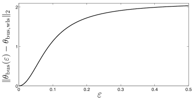
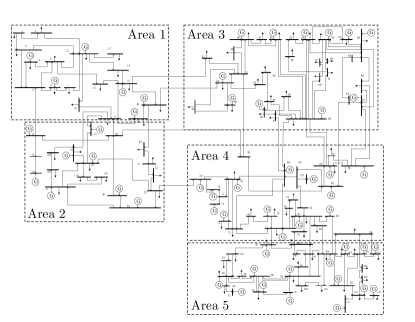
Figure 2: In Fig. 2, the normalized euclidean norm of the error vector $\theta_{\textup{bus}}(\varepsilon)-\theta_{\textup{bus,wls}}$ is plotted as a function of the parameter $\varepsilon$, where $\theta_{\textup{bus}}(\varepsilon)$ is the estimation vector computed according to Theorem 3.2, and $\theta_{\textup{bus,wls}}$ is the minimum variance estimate of $\theta_{\textup{bus}}$. As $\varepsilon$ decreases, the vector $\theta_{\textup{bus}}(\varepsilon)$ converges to the minimum variance estimate $\theta_{\textup{bus,wls}}$. In Fig. 2, the IEEE 118 bus system has been divided into $5$ areas. Each area is monitored and operated by a control center. The control centers cooperate to estimate the state and to assess the functionality of the whole network.

In order to demonstrate the advantage of our decentralized estimation algorithm, we assume the presence of $5$ control centers in the network of Fig. 1, each one responsible for a subpart of the entire network. The situation is depicted in Fig. 2. Assume that each control center measures the real power injected at the buses in its area, and let $z_{i}=P_{\textup{bus,i}}-v_{i}$, with $\operatorname{\mathbb{E}}[v_{i}]=0$ and $\operatorname{\mathbb{E}}[v_{i}v_{i}^{\mathsf{T}}]=\sigma_{i}^{2}I$, be the measurements vector of the $i$-th area. Finally, assume that the $i$-th control center knows the matrix $H_{\textup{bus,i}}$ such that $z_{i}=H_{\textup{bus,i}}\theta_{\textup{bus}}+v_{i}$. Then, as discussed in Section 3, the control centers can compute an optimal estimate of $\theta_{\textup{bus}}$ by means of Algorithm 1 or 2. Let $n_{i}$ be the number of measurements of the $i$-th area, and let $N=\sum_{i=1}^{5}n_{i}$. Notice that, with respect to a centralized computation of the minimum variance estimate of the state vector, our estimation procedure obtains the same estimation accuracy while requiring a smaller computation burden and memory requirement. Indeed, the $i$-th monitor uses $n_{i}$ measurements instead of $N$. Let $\bar{N}$ be the maximum number of measurements that, due to hardware or numerical contraints, a control center can efficiently handle for the state estimation problem. In Fig. 3, we increase the number of measurements taken by a control center, so that $n_{i}\leq\bar{N}$, and we show how the accuracy of the state estimate increases with respect to a single control center with $\bar{N}$ measurements.

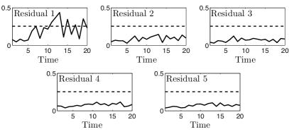
Figure 3: For a fixed value of $\varepsilon$, Fig. 3 shows the average (over 100 tests) of the norm of the error (with respect to the network state) of the estimate obtained by means of Algorithm 1. The estimation error decreases with the number of measurements. Because of the presence of several control centers, our distributed algorithm processes more measurements (up to $5\bar{N}$) while maintaining the same (or smaller) computational complexity of a centralized estimation (with $\bar{N}$ measurements). Fig. 3 shows the residual functions computed by the $5$ control centers. Since the first residual is greater than the threshold value, the presence of false data is correctly detected by the first control center. A form of regional identification is possible by simple identifying the residuals above the security threshold.

To conclude this section, we consider a security application, in which the control centers aim at detecting the presence of false data among the network measurements via distributed computation. For this example, we assume that each control center mesures the real power injection as well the current magnitude at some of the buses of its area. By doing so, a sufficient redundancy in the measurements is obtained for the detection to be feasible [1]. Suppose that the measurements of the power injection at the first bus of the first area is corrupted by a malignant agent. To be more precise, let the measurements vector of the first area be $\bar{z}_{i}=z_{i}+e_{1}w_{i}$, where $e_{1}$ is the first canonical vector, and $w_{i}$ is a random variable. For the simulation we choose $w_{i}$ to be uniformly distributed in the interval $[0,w_{\textup{max}}]$, where $w_{\textup{max}}$ corresponds approximately to the $10\%$ of the nominal real injection value. In order to detect the presence of false data among the measurements, the control centers implement Algorithm 3, where, being $H$ the measurements matrix, and $\sigma$, $\Sigma$ the noise standard deviation and covariance matrix, the threshold value $\Gamma$ is chosen as $2\sigma\|I-H(H^{\mathsf{T}}\Sigma^{-1}H)^{-1}H^{\mathsf{T}}\Sigma^{-1}\|_{\infty}$. The residual functions $\|z_{i}-H\hat{x}\|_{\infty}$ are reported in Fig. 3. Observe that, since the first residual is greater than the threshold $\Gamma$, the control centers successfully detect the false data. Regarding the identification of the corrupted measurements, we remark that a regional identification may be possible by simply analyzing the residual functions. In this example, for instance, since the residuals $\{2,\dots,5\}$ are below the threshold value, the corrupted data is likely to be among the measurements of the first area. This important aspect is left as the subject of future research.

5.2 Scalability property of our finite-memory estimation technique

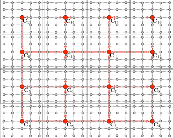
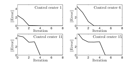
Figure 4: In Fig. 4, a two dimensional power grid with $400$ buses. The network is operated by $16$ control centers, each one responsible for a different subnetwork. Control centers cooperate through the red communication graph. Fig. 4 shows the norm of the estimation error of the local subnetwork as a function of the number of iterations of Algorithm 2. The considered monitors are $C_{1}$ ,$C_{6}$, $C_{11}$, and $C_{15}$. As predicted by Theorem 4.1, the local estimation error becomes negligible before the termination of the algorithm.

Consider an electrical network with $(ab)^{2}$ buses, where $a,b\in{\mathbb{N}}$. Let the buses interconnection structure be a two dimensional lattice, and let $G$ be the graph whose vertices are the $(ab)^{2}$ buses, and whose edges are the network branches. Let $G$ be partitioned into $b^{2}$ identical blocks containing $a^{2}$ vertices each, and assume the presence of $b^{2}$ control centers, each one responsible for a different network part. We assume the control centers to be interconnected through an undirected graph. In particular, being $V_{i}$ the set of buses assigned to the control center $\textup{C}_{i}$, we let the control centers $\textup{C}_{i}$ and $\textup{C}_{j}$ be connected if there exists a network branch linking a bus in $V_{i}$ to a bus in $V_{j}$. An example with $b=4$ and $a=5$ is in Fig. 4. In order to show the effectiveness of our approximation procedure, suppose that each control center $\textup{C}_{i}$ aims at estimating the vector of the voltage angles at the buses in its region. We assume also that the control centers cooperate, and that each of them receives the measurements of the real power injected at only the buses in its region. Algorithm 2 is implemented by the control centers to solve the estimation problem. In Fig. 4 we report the estimation error during the iterations of the algorithm. Notice that, as predicted by Theorem 4.1, each leader possess a good estimate of the state of its region before the termination of the algorithm.

6 Conclusion

Two distributed algorithms for network control centers to compute the minimum variance estimate of the network state given noisy measurements have been proposed. The two methods differ in the mode of cooperation of the control centers: the first method implements an incremental mode of cooperation, while the second uses a diffusive interaction. Both methods converge in finite time, which we characterize, and they require only local measurements and model knowledge to be implemented. Additionally, an asynchronous and scalable implementation of our diffusive estimation method has been described, and its efficiency has been shown through a rigorous analysis and through a practical example. Based on these estimation methods, an algorithm to detect cyber-attacks against the network measurements has also been developed, and its detection performance has been characterized.

APPENDIX

6.1 Proof of Theorem 3.1

Let $H^{i}=[H_{1}^{\mathsf{T}}\enspace\cdots\enspace H_{i}^{\mathsf{T}}]^{\mathsf{T}}$, $z^{i}=[z_{1}^{\mathsf{T}}\enspace\cdots\enspace z_{i}^{\mathsf{T}}]^{\mathsf{T}}$. We show by induction that $z^{i}=H^{i}\hat{x}_{i}$, $K_{i}=\operatorname{Basis}(\operatorname{Ker}(H^{i}))$, and $\hat{x}_{i}\perp\operatorname{Ker}(H^{i})$. Note that the statements are trivially verified for $i=1$. Suppose that they are verified up to $i$, then we need to show that $K_{i+1}=\operatorname{Basis}(\operatorname{Ker}(H^{i+1}))$, $\hat{x}_{i+1}\perp\operatorname{Ker}(H^{i+1})$, and $z^{i+1}=H^{i+1}\hat{x}_{i+1}$.

We start by proving that $K_{i+1}=\operatorname{Basis}(\operatorname{Ker}(H^{i+1}))$. Observe that $\operatorname{Ker}(K_{i})=0$ for all $i$, and that

$$\operatorname{Ker}(H_{i+1}K_{i})=\{v:K_{i}v\in\operatorname{Ker}(H_{i+1})\}.$$ (A-1)

Hence,

$$\operatorname{Im}(K_{i+1}) =\operatorname{Im}(K_{i}\operatorname{Ker}(H_{i+1}K_{i}))=\operatorname{Im}(K_{i})\cap\operatorname{Ker}(H_{i+1})=\operatorname{Ker}(H^{i})\cap\operatorname{Ker}(H_{i+1})=\operatorname{Ker}(H^{i+1}).$$

We now show that $x_{i+1}\perp\operatorname{Ker}(H^{i+1})$, which is equivalent to

$$\hat{x}_{i+1}=(\hat{x}_{i}+K_{i}(H_{i+1}K_{i})^{\dagger}(z_{i+1}-H_{i+1}\hat{x}_{i}))\in\operatorname{Ker}(H^{i+1})^{\perp}.$$

Note that

$$\operatorname{Ker}(H^{i+1})\subseteq\operatorname{Ker}(H^{i})\enspace\Leftrightarrow\enspace\operatorname{Ker}(H^{i+1})^{\perp}\supseteq\operatorname{Ker}(H^{i})^{\perp}.$$

By the induction hypothesis we have $\hat{x}_{i}\in\operatorname{Ker}(H^{i})^{\perp}$, and hence $\hat{x}_{i}\in\operatorname{Ker}(H^{i+1})^{\perp}$. Therefore, we need to show that

$$K_{i}(H_{i+1}K_{i})^{\dagger}(z_{i+1}-H_{i+1}\hat{x}_{i})\in\operatorname{Ker}(H^{i+1})^{\perp}.$$

Let $w=(H_{i+1}K_{i})^{\dagger}(z_{i+1}-H_{i+1}\hat{x}_{i})$, and notice that $w\in\operatorname{Ker}(H_{i+1}K_{i})^{\perp}$ due to the properties of the pseudoinverse operation. Suppose that $K_{i}w\not\in\operatorname{Ker}(H_{i+1})^{\perp}$. Since $\operatorname{Ker}(K_{i})=\{0\}$, the vector $w$ can be written as $w=w_{1}+w_{2}$, where $K_{i}w_{1}\in\operatorname{Ker}(H_{i+1})^{\perp}$ and $K_{i}w_{2}=K_{i}w-K_{i}w_{1}\neq 0$, $K_{i}w_{2}\in\operatorname{Ker}(H_{i+1})$. Then, it holds $H_{i+1}K_{i}w_{2}=0$, and hence $w_{2}\in\operatorname{Ker}(H_{i+1}K_{i})$, which contradicts the hypothesis $w\in\operatorname{Ker}(H_{i+1}K_{i})^{\perp}$. Finally $K_{i}w\in\operatorname{Ker}(H_{i+1})^{\perp}\subseteq\operatorname{Ker}(H^{i+1})^{\perp}$.

We now show that $z^{i+1}=H^{i+1}\hat{x}_{i+1}$. Because of the consistency of the system of linear equations, and because $z^{i}=H^{i}\hat{x}_{i}$ by the induction hypothesis, there exists a vector $v_{i}\in\operatorname{Ker}(H^{i})=\operatorname{Im}(K_{i})$ such that $z^{i+1}=H^{i+1}(\hat{x}_{i}+v_{i})$, and hence that $z_{i+1}=H_{i+1}(\hat{x}_{i}+v_{i})$. We conclude that $(z_{i+1}-H_{i+1}\hat{x}_{i})\in\operatorname{Im}(H_{i+1}K_{i})$, and finally that $z^{i+1}=H^{i+1}\hat{x}_{i+1}$.

6.2 Proof of Theorem 3.2

Before proceeding with the proof of the above theorem, we recall the following fact in linear algebra.

Lemma 6.1

Let $H\in\mathbb{R}^{n\times m}$. Then $\operatorname{Ker}((H^{\dagger})^{\mathsf{T}})=\operatorname{Ker}(H)$.

We first show that $\operatorname{Ker}((H^{\dagger})^{\mathsf{T}})\subseteq\operatorname{Ker}(H)$. Recall from [2] that $H=HH^{\mathsf{T}}(H^{\dagger})^{\mathsf{T}}$. Let $x$ be such that $(H^{\dagger})^{\mathsf{T}}x=0$, then $Hx=HH^{\mathsf{T}}(H^{\dagger})^{\mathsf{T}}x=0$, so that $\operatorname{Ker}((H^{\dagger})^{\mathsf{T}})\subseteq\operatorname{Ker}(H)$. We now show that $\operatorname{Ker}(H)\subseteq\operatorname{Ker}((H^{\dagger})^{\mathsf{T}})$. Recall that $(H^{\dagger})^{\mathsf{T}}=(H^{\mathsf{T}})^{\dagger}=(HH^{\mathsf{T}})^{\dagger}H$. Let $x$ be such that $Hx=0$, then $(H^{\dagger})^{\mathsf{T}}x=(HH^{\mathsf{T}})^{\dagger}Hx=0$, so that $\operatorname{Ker}(H)\subseteq\operatorname{Ker}((H^{\dagger})^{\mathsf{T}})$, which concludes the proof. We are now ready to prove Theorem 3.2. The first property follows directly from [2] (cfr. page 427). To show the second property, observe that $C^{\dagger}=\frac{1}{\varepsilon}((I-HH^{\dagger})B)^{\dagger}$, so that

$$\lim_{\varepsilon\rightarrow 0^{+}}\varepsilon D=0.$$

For the theorem to hold, we need to verify that

$$H^{\dagger}-H^{\dagger}B((I-HH^{\dagger})B)^{\dagger}=(H^{\mathsf{T}}\Sigma^{-1}H)^{-1}H^{\mathsf{T}}\Sigma^{-1},$$

or, equivalently, that

$$\begin{split}&\left(H^{\dagger}-H^{\dagger}B((I-HH^{\dagger})B)^{\dagger}\right)HH^{\dagger}=(H^{\mathsf{T}}\Sigma^{-1}H)^{-1}H^{\mathsf{T}}\Sigma^{-1}HH^{\dagger},\end{split}$$ (A-2)

and

$$\begin{split}&\left(H^{\dagger}-H^{\dagger}B((I-HH^{\dagger})B)^{\dagger}\right)(I-HH^{\dagger})=(H^{\mathsf{T}}\Sigma^{-1}H)^{-1}H^{\mathsf{T}}\Sigma^{-1}(I-HH^{\dagger}).\end{split}$$ (A-3)

Consider equation (A-2). After simple manipulation, we have

$$H^{\dagger}-H^{\dagger}B((I-HH^{\dagger})B)^{\dagger}HH^{\dagger} =H^{\dagger},$$

so that we need to show only that

$$H^{\dagger}B((I-HH^{\dagger})B)^{\dagger}HH^{\dagger} =0.$$

Recall that for a matrix $W$ it holds $W^{\dagger}=(W^{\mathsf{T}}W)^{\dagger}W^{\mathsf{T}}$. Then the term $((I-HH^{\dagger})B)^{\dagger}HH^{\dagger}$ equals

$$\left(((I-HH^{\dagger})B)^{\mathsf{T}}((I-HH^{\dagger})B)\right)^{\dagger}B^{\mathsf{T}}(I-HH^{\dagger})HH^{\dagger}=0,$$

because $(I-HH^{\dagger})HH^{\dagger}=0$. We conclude that equation (A-2) holds. Consider now equation (A-3). Observe that $HH^{\dagger}(I-HH^{\dagger})=0$. Because $B$ has full row rank, and $\Sigma=BB^{\mathsf{T}}$, simple manipulation yields

$$-H^{\mathsf{T}}(BB^{\mathsf{T}})^{-1}HH^{\dagger}B\left[(I-HH^{\dagger})B\right]^{\dagger}(I-HH^{\dagger})B=H^{\mathsf{T}}(BB^{\mathsf{T}})^{-1}(I-HH^{\dagger})B,$$

and hence

$$H^{\mathsf{T}}(BB^{\mathsf{T}})^{-1}\left\{I+HH^{\dagger}B\left[(I-HH^{\dagger})B\right]^{\dagger}\right\}(I-HH^{\dagger})B=0.$$

Since $HH^{\dagger}=I-(I-HH^{\dagger})$, we obtain

$$H^{\mathsf{T}}(BB^{\mathsf{T}})^{-1}B\left[(I-HH^{\dagger})B\right]^{\dagger}(I-HH^{\dagger})B=0.$$

A sufficient condition for the above equation to be true is

$$\left(\left[(I-HH^{\dagger})B\right]^{\dagger}\right)^{\mathsf{T}}B^{\mathsf{T}}(BB^{\mathsf{T}})^{-1}H=0.$$

From Lemma 6.1 we have.

$$\operatorname{Ker}\left(\left(\left[(I-AA^{\dagger})B\right]^{\dagger}\right)^{\mathsf{T}}\right)=\operatorname{Ker}((I-AA^{\dagger})B).$$

Since

$$(I-HH^{\dagger})BB^{\mathsf{T}}(BB^{\mathsf{T}})^{-1}H=(I-HH^{\dagger})H=0,$$

we have that

$$H^{\mathsf{T}}(BB^{\mathsf{T}})^{-1}B\left[(I-HH^{\dagger})B\right]^{\dagger}(I-HH^{\dagger})B=0,$$

and that equation (A-3) holds. This concludes the proof.

References

- [1] A. Abur and A. G. Exposito. Power System State Estimation: Theory and Implementation. CRC Press, 2004.
- [2] D. S. Bernstein. Matrix Mathematics. Princeton University Press, 2 edition, 2009.
- [3] R. Carli, A. Chiuso, L. Schenato, and S. Zampieri. Distributed Kalman filtering based on consensus strategies. IEEE Journal on Selected Areas in Communications, 26(4):622–633, 2008.
- [4] F. S. Cattivelli, C. G. Lopes, and A. H. Sayed. Diffusion recursive least-squares for distributed estimation over adaptive networks. IEEE Transactions on Signal Processing, 56(5):1865–1877, 2008.
- [5] F. S. Cattivelli and A. H. Sayed. Diffusion strategies for distributed Kalman filtering and smoothing. IEEE Transactions on Automatic Control, 55(9):2069–2084, 2010.
- [6] Y. Censor. Row-action methods for huge and sparse systems and their applications. SIAM Review, 23(4):444–466, 1981.
- [7] S. Demko, W. F. Moss, and P. W. Smith. Decay rates for inverses of band matrices. Mathematics of Computation, 43(168):491–499, 1984.
- [8] D. M. Falcao, F. F. Wu, and L. Murphy. Parallel and distributed state estimation. IEEE Transactions on Power Systems, 10(2):724–730, 1995.
- [9] C. D. Godsil and G. F. Royle. Algebraic Graph Theory, volume 207 of Graduate Texts in Mathematics. Springer, 2001.
- [10] G. H. Golub and C. F. van Loan. Matrix Computations. Johns Hopkins University Press, 2 edition, 1989.
- [11] R. Gordon, R. Bender, and G. T. Herman. Algebraic reconstruction techniques (ART) for three-dimensional electron microscopy and x-ray photography. Journal of theoretical Biology, 29(3):471–481, 1970.
- [12] W. Jiang, V. Vittal, and G. T. Heydt. A distributed state estimator utilizing synchronized phasor measurements. IEEE Transactions on Power Systems, 22(2):563–571, 2007.
- [13] S. Kaczmarz. Angenäherte Auflösung von Systemen linearer Gleichungen. Bull. Acad. Polon. Sci. Lett. A, 35:355–357, 1937.
- [14] Y. Liu, M. K. Reiter, and P. Ning. False data injection attacks against state estimation in electric power grids. In ACM Conference on Computer and Communications Security, pages 21–32, Chicago, IL, USA, November 2009.
- [15] C. G. Lopes and A. H. Sayed. Incremental adaptive strategies over distributed networks. IEEE Transactions on Signal Processing, 55(8):4064–4077, 2007.
- [16] C. G. Lopes and A. H. Sayed. Diffusion least-mean squares over adaptive networks: Formulation and performance analysis. IEEE Transactions on Signal Processing, 56(7):3122–3136, 2008.
- [17] D. G. Luenberger. Optimization by Vector Space Methods. Wiley, 1969.
- [18] J. Meserve. Sources: Staged cyber attack reveals vulnerability in power grid. http://cnn.com, September 26, 2007.
- [19] A. Monticelli. State Estimation in Electric Power Systems: A Generalized Approach. Springer, 1999.
- [20] NERC. Final Report on the August 14, 2003 Blackout in the United States and Canada: Causes and Recommendations, April 2004. Available at http://www.nerc.com/filez/blackout.html.
- [21] F. Pasqualetti, R. Carli, A. Bicchi, and F. Bullo. Distributed estimation and detection under local information. In IFAC Workshop on Distributed Estimation and Control in Networked Systems, pages 263–268, Annecy, France, September 2010.
- [22] M. G. Rabbat and R. D. Nowak. Quantized incremental algorithms for distributed optimization. IEEE Journal on Selected Areas in Communications, 23(4):798–808, 2005.
- [23] C. Rakpenthai, S. Premrudeepreechacharn, S. Uatrongjit, and N. R. Watson. Measurement placement for power system state estimation using decomposition technique. Electric Power Systems Research, 75(1):41–49, 2005.
- [24] A. H. Sayed and C. G. Lopes. Adaptive processing over distributed networks. IEICE Transactions on Fundamentals of Electronics, Communications and Computer Sciences, E90-A(8):1504–1510, 2007.
- [25] I. Schizas, A. Ribeiro, and G. Giannakis. Consensus in ad hoc WSNs with noisy links - Part I: Distributed estimation of deterministic signals. IEEE Transactions on Signal Processing, 56(1):350–364, 2007.
- [26] I. D. Schizas, G. Mateos, and G. B. Giannakis. Distributed LMS for consensus-based in-network adaptive processing. IEEE Transactions on Signal Processing, 57(6):2365–2382, 2009.
- [27] F. C. Schweppe and J. Wildes. Power system static-state estimation, Part I: Exact model. IEEE Transactions on Power Apparatus and Systems, 89(1):120–125, 1970.
- [28] F. C. Schweppe and J. Wildes. Power system static-state estimation, Part II: Approximate model. IEEE Transactions on Power Apparatus and Systems, 89(1):125–130, 1970.
- [29] F. C. Schweppe and J. Wildes. Power system static-state estimation, Part III: Implementation. IEEE Transactions on Power Apparatus and Systems, 89(1):130–135, 1970.
- [30] M. Shahidehpour and Y. Wang. Communication and Control in Electric Power Systems: Applicationsc of Parallel and Distributed Processing. Wiley-IEEE Press, 2003.
- [31] S. S. Stankovic, M. S. Stankovic, and D. M. Stipanovic. Consensus based overlapping decentralized estimation with missing observations and communication faults. Automatica, 45(6):1397–1406, 2009.
- [32] K. Tanabe. Projection method for solving a singular system of linear equations and its applications. Numerische Mathematik, 17(3):203–214, 1971.
- [33] L. Xie, Y. Mo, and B. Sinopoli. False data injection attacks in electricity markets. In IEEE Int. Conf. on Smart Grid Communications, pages 226–231, Gaithersburg, MD, USA, October 2010.
- [34] L. Zhao and A. Abur. Multi area state estimation using synchronized phasor measurements. IEEE Transactions on Power Systems, 20(2):611–617, 2005.