Finite-size effects in Anderson localization of one-dimensional Bose-Einstein condensates

Abstract

We investigate the disorder-induced localization transition in Bose-Einstein condensates for the Anderson and Aubry-André models in the non-interacting limit using exact diagonalization. We show that, in addition to the standard superfluid fraction, other tools such as the entanglement and fidelity can provide clear signatures of the transition. Interestingly, the fidelity exhibits good sensitivity even for small lattices. Effects of the system size on these quantities are analyzed in detail, including the determination of a finite-size-scaling law for the critical disorder strength in the case of the Anderson model.

I Introduction

Localization of waves in a disordered medium was first predicted by Anderson Anderson in the context of non-interacting electrons in a random crystal. Recently, developments in the research into ultracold atomic gases have enlarged the possibilities for studying Anderson localization in new systems. A breakthrough in the area was the experimental realization of Anderson localization of a Bose-Einstein condensate (BEC) in two different kinds of disordered optical potentials Billy08 ; Roati08 : Billy et al. Billy08 employed a BEC of $\,{}^{87}$Rb atoms in the presence of a controlled disorder produced by a laser speckle, while Roati et al. Roati08 utilized a BEC of essentially non-interacting ³⁹K atoms in combination with a one-dimensional quasi-periodic lattice to observe Anderson localization.

Subsequently, this issue has been attracting increasing interest from both the experimental and theoretical communities. From the experimental point of view, a variety of techniques have been implemented, such as bichromatic optical lattices Roati08 ; roth ; fallani , speckle laser patterns Billy08 ; Inguscio_speckle ; aspect_1d_disorder , and disordered cold atom lattices castin . Theoretically, different approaches such as a variational method adhikari1 , quantum Monte Carlo simulation Haas_QMC ; Zimanyi_QMC , exact diagonalization roth ; Sengstock_exact ; pugatch ; Tsubota_exact , renormalization group Singh_RG ; Giamarchi_RG , density-matrix renormalization group Zwerger_DMRG ; iucci_DMRG ; roux_DMRG , mean-field approximations Buonsante_1d_MFT ; Lewenstein_Bose_anderson_glass ; Sheshadri ; dalfovo , and a perturbative treatment orso , among others, have been explored in this context of disordered ultracold atoms.

The usual model for bosons on a lattice utilizes the so-called Bose-Hubbard Hamiltonian, with the general form

$$H=\sum_{i}\varepsilon_{i}n_{i}+\Omega\sum_{\langle ij\rangle}(a^{{\dagger}}_{i}a_{j}+a^{{\dagger}}_{j}a_{i})+\frac{U}{2}\sum_{i}n_{i}(n_{i}-1)\,,$$ (1)

with the standard notation for creation, annihilation, and number operators for bosons at lattice sites. Each site is considered to have a single bound state of energy $\varepsilon_{i}$, the hopping between sites is restricted to nearest neighbors, with amplitude $\Omega$, and $U$ is a local repulsive interaction.

Randomness is introduced via the values of $\varepsilon_{i}$. These values can have a truly random (usually uniform) distribution in the range $-\Delta/2\leq\varepsilon_{i}\leq\Delta/2$, which characterizes the Anderson model Anderson . Alternatively, they can vary periodically with a period incommensurate with the lattice spacing. This is the case in the Aubry-André (AA) model aa for which the energies, in the one-dimensional case, are written as $\varepsilon_{i}=\Delta\cos(2\pi\beta i)$, where $\beta=(1+\sqrt{5})/2$ is the golden ratio, and $i$ assumes integer values from 1 to $L$ (the system size in units of the lattice spacing). Experimentally, speckle patterns can be modeled by the Anderson model, while quasi-periodic potentials can be described by the AA model.

The phenomenology of model (1) at low temperatures involves Bose-Einstein condensation, superfluidity, a Mott (gapped) phase, and Anderson localization, depending on the relative values of $\Omega$, $U$, and $\Delta$ Fisher89 . Theoretical studies of such a rich phenomenology are faced with the usual challenges of interacting many-body problems. For arbitrary interaction strengths perturbation theory cannot be used, which more or less restricts the approach to numerical solutions on finite-size lattices. Then, finite-size effects tend to smear out the sharp phase boundaries expected in the thermodynamic limit. This is true even for the pure Anderson transition in the non-interacting limit. For instance, in his original paper Anderson Anderson proved that his model presents localization for any $\Delta>0$ in one dimension, while Aubry and André aa proved that in their model localization only occurs for $\Delta\geq 2$, but these critical values are not clearly seen in small lattices.

Our aim in this paper is to discuss in detail the effects of finite size in the non-interacting limit for a one-dimensional lattice. We focus on the size dependence of quantities that provide signatures of quantum phase transitions (QPTs), here applied to Anderson localization. In addition to the superfluid fraction, common in studies of Bose-Einstein condensates, we also employ quantities borrowed from quantum information theory, like entanglement and fidelity nielsen . All of these quantities allow us to obtain the correct thermodynamic limit of the critical disorder strength for both Anderson and Aubry-André models. In particular, we are able to show that the critical disorder strength in the Anderson model obeys a scaling law with the system size.

II Localization transition

We consider one-dimensional lattices of $L$ sites, and perform exact numerical diagonalization of the Hamiltonian matrix, obtaining a chosen number of lowest-energy eigenvalues, and the corresponding eigenvectors. We will focus only on ground-state results. Since interaction is not taken into account here, we restrict our numerical calculations to a single particle. When evaluating the quantities of interest for the Anderson model, it is necessary to average over a large number of random configurations of the local energies in order to have physically meaningful results.

For each lattice size, we calculate the superfluid fraction, ground-state entanglement and fidelity, as discussed in detail below. This is done for a wide range of disorder strength values, with the aim of determining a critical value above which the states are localized. Throughout the paper, energy quantities (like $\Delta$) are measured in units of the tunneling amplitude $\Omega$, while the lattice size $L$ is expressed in units of the lattice spacing, which is equivalent to the number of sites.

II.1 Superfluid fraction

The ground state of a uniform Bose-Einstein condensate should be superfluid. There is some controversy as to whether this remains true in the non-interacting limit. As discussed by Lieb et al. lieb , if one defines a superfluid as a fluid that does not respond to an external velocity field (e.g., rotation of the container walls), then the ideal Bose gas is a perfect superfluid in its ground state. This is the approach we adopt here. On the other hand, the presence of disorder tends to alter the nature of the quantum states, which become no longer extended over the entire system, but localized over a finite distance. Then, the so called superfluid fraction (here denoted by $f_{s}$) can signal whether the states are extended ($f_{s}\neq 0$) or not ($f_{s}=0$).

The superfluid fraction for a discrete lattice system is proportional to the difference in ground-state energy between the systems with periodic and with twisted boundary conditions roth . Instead, we may keep periodic boundary conditions and use a twisted Hamiltonian

$$H_{\theta}=\sum_{i=1}^{L}\varepsilon_{i}n_{i}+\Omega\sum_{\langle ij\rangle}(a^{{\dagger}}_{i}a_{j}e^{-i\frac{\theta}{L}}+a^{{\dagger}}_{j}a_{i}e^{i\frac{\theta}{L}})\,,$$ (2)

where $\theta$ is the twist angle. Ground-state energies of the Hamiltonian (2) are calculated for $\theta=0$ ($E_{0}$) as well as for finite $\theta$ ($E_{\theta}$), and the superfluid fraction is given by roth

$$f_{s}=\frac{L^{2}}{N\Omega}\frac{(E_{\theta}-E_{0})}{\theta^{2}}\,,$$ (3)

being independent of the twist angle $\theta$ as long as $\theta<<\pi$. In practice, $f_{s}$ remains the same even for twist angles that are a significant fraction of $\pi$. Typically, we use $\theta=0.1$ in our numerical calculations.

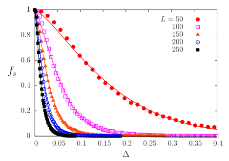
Figure 1: (Color online) Average superfluid fraction in the Anderson model as a function of the disorder strength $\Delta$ for different lattice sizes. The averages were calculated from 5000 random configurations of the potential. The lines correspond to fittings with Eq. (4).

In Fig. 1 we show the superfluid fraction for the Anderson model as a function of disorder strength for different lattice sizes. When $\Delta=0$ we always have $f_{s}=1$, i.e., the system is in a superfluid phase. For large enough $\Delta$ we have $f_{s}\to 0$, and the ground-state is localized.

We define a characteristic value $\Delta_{L}$ of the disorder strength for each lattice size by observing that the superfluid-fraction curves are well fitted by the function

$$f_{s}\simeq e^{(-\frac{\Delta}{\Delta_{L}})^{\alpha}}\,.$$ (4)

For all lattice sizes $L$ we find that the fitting parameter $\alpha$ has approximately the same value $\alpha\simeq\frac{4}{3}$. Lines in Figure 1 show the fittings with Eq. (4) while symbols are the corresponding values obtained by the numerical solution. Fig. 1 seems to indicate that $\Delta_{L}\to 0$ when $L\to\infty$, as expected. This behavior will be verified in Sec. III through a finite-size-scaling analysis.

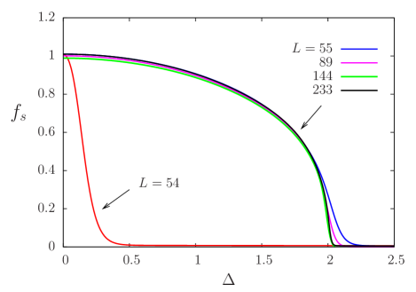
Figure 2: (Color online) Superfluid fraction in the AA model as a function of the potential amplitude $\Delta$ for chosen lattice sizes. The expected critical value $\Delta_{c}=2$ is well verified for suitably chosen lattice sizes, but not for others (e.g., $L=54$ in this figure), as discussed in the text. The lines indicated at the top right corner are essentially indistinguishable, except near $\Delta=2$, where rounding is more noticeable for smaller sizes.

Figure 2 shows the superfluid fraction for the Aubry-André model as a function of the “disorder strength” $\Delta$ for different lattice sizes. Actually, $\Delta$ is the amplitude of the Aubry-André potential, i.e., the incommensurate periodic modulation of local energies. We can see that $f_{s}(\Delta)=0$ for $\Delta$ larger than a characteristic $\Delta_{L}$, with $\Delta_{L}\approx 2$, consistent with the expected critical value $\Delta_{c}=2$. However, this happens for certain lattice sizes, but for other values of $L$ the behavior of $f_{s}$ with $\Delta$ is completely different, even for very similar sizes, as exemplified for $L=54$ and 55 in Fig. 2. The reason for this apparently puzzling feature lies in the mismatching between periodic boundary conditions with integer period $L$ and the Aubry-André potential with irrational period $\beta^{-1}$. One can verify that $\Delta_{L}\approx 2$ occurs when $L$ belongs to the sequence of Fibonacci numbers harper . The first members of this sequence, for $L\geq 8$, are 8, 13, 21, 34, 55, 89, 144,…. The ratio between two consecutive Fibonacci numbers approaches the golden ratio when these numbers become very large. For small lattice sizes it is better to redefine the parameter $\beta$ to be such a ratio of Fibonacci numbers. We do this in order to get better results for smaller sizes like $L=8$ or 13, which become relevant for numerical solutions in the presence of interactions. It is worth mentioning that departure from the critical $\Delta_{c}=2$ was observed in the experiments of Roati et al. Roati08 . They find localization for $\Delta\geq 7$, using an incommensurate potential with $\beta\simeq 1.1972$. This value of $\beta$, being significantly different from a ratio of consecutive Fibonacci numbers (the golden ratio is $\sim 1.6180$), does not ensure the duality condition harper that yields $\Delta_{c}=2$.

II.2 Entanglement

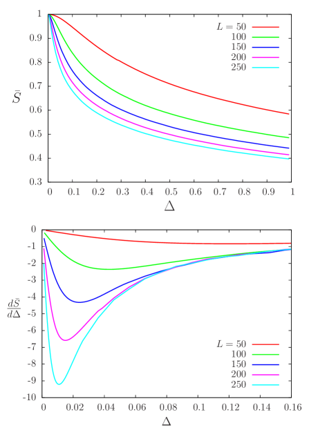
Figure 3: (Color online) Top: Average entanglement as a function of the disorder strength $\Delta$ for different lattice sizes in the Anderson model. Averages were calculated from 5000 random configurations of the potential. Bottom: Derivative of the entanglement with respect to the disorder strength $\Delta$ for the same sizes. The location of its minimum for a given system size $L$ is taken as the corresponding critical disorder strength $\Delta_{L}$. On both panels, curves are associated to increasing lattice sizes from top to bottom.

The concept of quantum entanglement can be used to study localization if we choose a basis for the Hilbert space composed of states that are localized at each of the lattice sites. Then, a fully extended ground-state will have maximum entanglement of the basis states. In the opposite limit, the entanglement will be zero for localization at a single site. So, the ground-state Shannon entropy is a good measure of entanglement. It is given by

$$S=-\sum_{i}p_{i}\log_{2}p_{i}\,,$$ (5)

where $p_{i}=|c_{i}|^{2}$, with $c_{i}$ representing the coefficient of the $i$-th basis state in the expansion of the ground-state vector $|\Psi_{0}\rangle$ stephan ; milburn . For a lattice of $L$ sites, the maximum value of $S$ is $\log_{2}L$, and occurs when all the $p_{i}$ are equal. We define $\bar{S}\equiv S/\log_{2}L$ as our measure of entanglement, whose maximum value will be $\bar{S}_{\mathrm{max}}=1$.

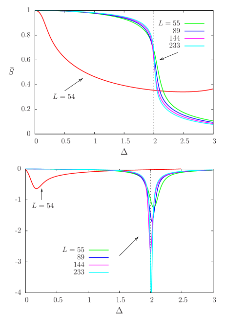
Figure 4: (Color online) Entanglement (top) as a function of the potential amplitude $\Delta$ for chosen lattice sizes in the AA model, and the corresponding derivative (bottom). Notice the sudden drop in the first case, and sharp minima in the second near the point $\Delta=2$, except for sizes that are not Fibonacci numbers, here exemplified by $L=54$. The size effect is better noticed in the bottom panel, where deeper minima correspond to larger lattice sizes.

In Fig. 3 (top panel) we show the ground-state entanglement $\bar{S}$ (averaged over disorder) for the Anderson model as a function of the disorder strength $\Delta$ for various lattice sizes $L$. We define the characteristic $\Delta_{L}$ in this case as the inflection point of the entanglement curve. It can be better visualized as the minimum in the derivative of $\bar{S}$ with respect to $\Delta$, as shown in the bottom panel of Fig. 3. Notice that the minimum moves toward $\Delta=0$ as $L$ increases. We will come back to this point in our finite-size-scaling analysis of Sec. III.

In the case of the AA model, the ground-state entanglement, when calculated for lattice sizes belonging to the Fibonacci series, shows a sudden drop near $\Delta=2$, as can be seen in Fig. 4 (top panel). This indicates that the derivative $d\bar{S}/d\Delta$ is again a good marker of the quantum phase transition. The bottom panel of Fig. 4 shows this derivative as a function of $\Delta$ for different lattice sizes. We can see a sharp minimum in the derivative essentially at $\Delta=2$, more or less independently of the lattice size. Here, the size effect appears mainly in the depth of the minimum, which increases dramatically with increasing size. A non Fibonacci size has been included for comparison in Fig. 4.

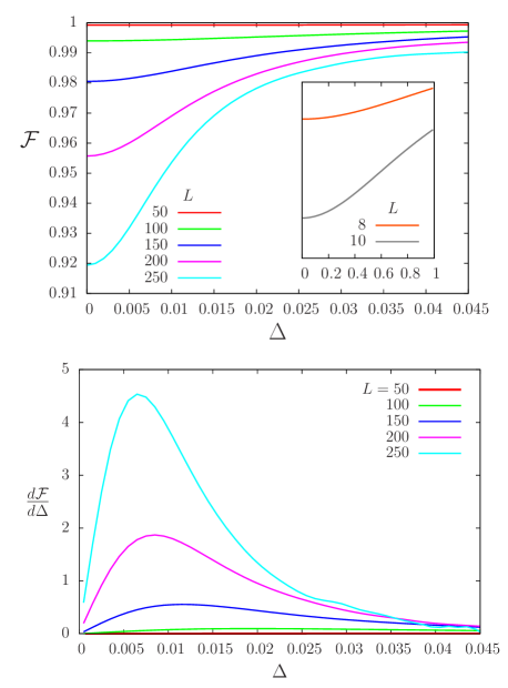
Figure 5: (Color online) Average ground-state fidelity (top) in the Anderson model as a function of disorder strength for different lattice sizes, and the corresponding derivative (bottom). Averages were calculated from 5000 random configurations of the potential. The top-panel inset shows (in a much smaller vertical scale) that the minimum at $\Delta=0$ exists even for small lattice sizes. The position of the maximum derivative for a given system size $L$ is taken as the critical disorder strength $\Delta_{L}$. Deeper minima of the fidelity (higher maxima of its derivative) correspond to larger lattice sizes.

II.3 Fidelity

The fidelity is a measure of how distinguishable two quantum states are. For pure states, it is defined as the absolute value of the overlap between these two states. We use here the scalar product of two ground-state vectors of Hamiltonians with slightly different values of $\Delta$, writing the fidelity as

$$\mathcal{F}(\Delta)=\Bigl{|}\langle\Psi_{0}(\Delta-\delta\Delta)|\Psi_{0}(\Delta+\delta\Delta)\rangle\Bigr{|}\,,$$ (6)

which has values between $0$ and $1$. Generically, the fidelity exhibits a minimum at a critical parameter value characterizing a QPT. We have checked that although the choice of $\delta\Delta$ affects the magnitude of the minimum, which can be made arbitrarily small, the value of $\Delta$ at which the minimum occurs is independent of $\delta\Delta$. Here we use $\delta\Delta=10^{-2}$ in all numerical calculations. In the case of the Anderson model, we perform the configuration average on $\mathcal{F}(\Delta)$, which means that both ground states are obtained for the same realization of the random local energies.

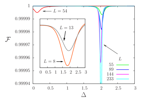
Figure 6: (Color online) Fidelity as a function of the disorder strength $\Delta$ for different lattice sizes. There is a sharp peak close to the point $\Delta=2$. The inset shows two small lattice sizes in a much narrower scale close to $\mathcal{F}=1$. We redefined $\beta$ as 13/8 and 21/13 for $L=8$ and 13, respectively. The curves indicated at the bottom right show minima that become more pronounced as $L$ increases.

The average ground-state fidelity for the Anderson model is shown in Fig. 5 (top panel) as a function of the disorder strength for different lattice sizes. It is interesting to notice that it has a minimum for all lattice sizes at $\Delta=0$, which is the expected critical disorder strength in one dimension for $L\to\infty$. The inset of Fig. 5 shows that this remains true even for sizes as small as $L=8$ and 10. The finite-size effect is noticeable in the minimum depth, which increases with $L$. Nevertheless, the minima are relatively broad, and an inflection point exists, which moves down in $\Delta$ as $L$ increases. This is better seen in the derivative of $\mathcal{F}(\Delta)$, shown in the bottom panel of Fig. 5. Similarly to what we observed for the superfluid fraction, here the maximum of $d\mathcal{F}/d\Delta$ locates a characteristic disorder strength $\Delta_{L}$ for each lattice size. A detailed analysis of the behavior of $\Delta_{L}$ for large $L$ will be presented in Sec. III.

The fact that $\mathcal{F}(\Delta)$ can signal the critical disorder strength for all lattice sizes is confirmed for the AA model. Figure 6 shows the fidelity as a function of $\Delta$ for different lattice sizes (all belonging to the Fibonacci series, except $L=54$). A sharp minimum appears very close to $\Delta=2$ for all the appropriate sizes, clearly indicating the localization transition. In this case, one does not extract more information from the derivative. The size effect is evident in the minimum depth, which is strongly dependent on the value of $L$.

We can observe that the ground-state fidelity is a very precise tool to indicate the localization transition, even for small lattice sizes. This is specially relevant in the interacting case, where numerical solutions must be restricted to relatively small sizes. It is interesting to mention that the concept of fidelity was also efficiently applied to identify quantum phase transitions in other models in the BEC scenario a1 ; a2 . For the Bose-Hubbard model without disorder, it was shown Buonsante_1d_MFT that the fidelity is a clearer indicator of a QPT than the entanglement.

III Finite-size scaling

In the previous section, we have seen that good signatures of the localization transition in the one-dimensional AA model are provided by the superfluid fraction, the ground-state entanglement, and the ground-state fidelity. All these quantities (or appropriate derivatives) correctly locate the critical amplitude of the incommensurate potential (equivalent to a “disorder strength”), more or less independently of lattice size, provided this size is not too small, and is chosen to be nearly commensurate with an integer number of oscillations of the AA potential.

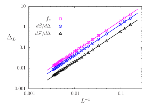
Figure 7: (Color online) Logarithmic plot of the critical disorder strength $\Delta_{L}$ in the Anderson model as a function of the lattice size, evaluated from superfluid fraction (squares), derivative of the entanglement (circles), and derivative of the fidelity(triangles). The lines are fittings to the scaling law (7), which is satisfied with an exponent $\gamma\approx 1.5$ and with $\Delta_{\infty}=0$ for all three quantities.

For the true Anderson model, however, the results are less clear-cut upon a simple direct visualization. We defined characteristic disorder strengths $\Delta_{L}$ in Sec. II, with different definitions depending on the physical quantity evaluated. In order to determine more quantitatively their size dependence, these different $\Delta_{L}$’s where calculated for lattice sites from 6 to 300, with random averages being performed typically over 5000 configurations. Despite the different definitions, if we make a log-log plot of $\Delta_{L}$ vs $L^{-1}$, as is done in Fig. 7, we see that in all the three cases (superfluid fraction, entanglement, and fidelity) the following scaling law is obeyed:

$$\Delta_{L}-\Delta_{\infty}=C\,L^{-\gamma}\,,$$ (7)

where $C$ and $\gamma$ are positive real numbers, and $\Delta_{\infty}$ is the critical disorder strength in the thermodynamic limit. Despite the fact that the prefactor $C$ in Eq. (7) differs for the three definitions of $\Delta_{L}$, we find the same exponent $\gamma\approx 1.5$ in all three cases, and the results are consistent with $\Delta_{\infty}=0$, in accordance with the exact value for Anderson localization in one dimension. It is also worth noticing in Fig. 7 that the scaling law (7) is satisfied even for lattice sizes as small as $L=6$.

IV Conclusions

We presented a detailed numerical study of disorder-induced localization in the one-dimensional Anderson and Aubry-André models of Bose-Einstein condensates. Through exact numerical diagonalization of the Hamiltonian matrix, we studied the superfluid fraction, entanglement, and fidelity as quantities that can signal the localization transition even at finite size. Here we restricted our analysis to the non-interacting limit in order to reach large lattice sizes. With this, we were able to verify that finite-size-scaling laws are obeyed by all the studied quantities in the case of the Anderson model, with a common exponent. In contrast, finite-size effects in the Aubry-André model are less pronounced, and mainly related to the incommensurability between the potential and the system size. If the incommensurate potential is tuned so that an integer number of periods nearly coincides with the system size, then the localization transition is fairly sharp at the critical potential strength.

Even though all the three quantities analyzed here show clear signatures of the localization transition, we find that the fidelity is less prone to finite-size effects. This makes it specially suited to be used in the interacting case, where numerical solutions are restricted, for practical reasons, to relatively small sizes.

Acknowledgments

We would like to thank CNPq - Conselho Nacional de Desenvolvimento Científico e Tecnológico (Brazil) for financial support.

References

- (1) P. W. Anderson, Phys. Rev. 109, 1492 (1958).
- (2) J. Billy, V. Josse, Z. Zuo, A. Bernard, B. Hambrecht, P. Lugan, D. Clément, L. Sanchez-Palencia, P. Bouyer and A. Aspect, Nature 453, 891 (2008).
- (3) G. Roati, C. D’Errico, L. Fallani, M. Fattori, C. Fort, M. Zaccanti, G. Modugno, M. Modugno, M. Inguscio, Nature 453, 895 (2008).
- (4) R. Roth and K. Burnett, Phys. Rev. A 68, 023604 (2003).
- (5) L. Fallani, J. E. Lye, V. Guarrera, C. Fort, and M. Inguscio, Phys. Rev. Lett. 98, 130404 (2007).
- (6) J. E. Lye, L. Fallani, M. Modugno, D. S. Wiersma, C. Fort and M. Inguscio, Phys. Rev. Lett. 95, 070401 (2005).
- (7) D. Clément, P. Bouyer, A. Aspect, L. Sanchez-Palencia, Phys. Rev. A 77, 033631 (2008).
- (8) U. Gavish and Y. Castin, Phys. Rev. Lett. 95, 020401 (2005).
- (9) Y. Cheng and S. K. Adhikari, Phys. Rev. A 82, 013631 (2010).
- (10) P. Sengupta, A. Raghavan, and S. Haas, New J. Phys. 9, 103 (2007).
- (11) R. T. Scalettar, G. G. Batrouni and G. T. Zimanyi, Phys. Rev. Lett. 66, 3144 (1991).
- (12) D.-S. Lühmann, K. Bongs, K. Sengstock, and D. Pfannkuche, Phys. Rev. A 77, 023620 (2008).
- (13) R. Pugatch, N. Bar-Gill, N. Katz, E. Rowen and N. Davidson, cond-mat/0603571v6.
- (14) P. Louis, M. Tsubota, J. Low Temp. Phys. 148, 351 (2007).
- (15) K.G. Singh and D.S. Rokhsar, Phys. Rev. B 46, 3002 (1992).
- (16) T. Giamarchi and H. J. Schulz, Phys. Rev. B 37, 325 (1988).
- (17) S. Rapsch, U. Scholhoöck, and W. Zwerger, Europhys. Lett. 46, 559 (1999).
- (18) C. Kollath, A. Iucci, T. Giamarchi, W. Hofstetter and U. Schollwöck, Phys. Rev. Lett. 97, 050402 (2006).
- (19) G. Roux, T. Barthel, I. P. McCulloch, C. Kollath, U. Schollwöck, and T. Giamarchi, Phys. Rev. A 78, 023628 (2008).
- (20) P. Buonsante, V. Penna, A. Vezzani and P. B. Blakie, Phys. Rev. A 76, 011602(R) (2007).
- (21) B. Damski, J. Zakrzewski, L. Santos, P. Zoller and M. Lewenstein, Phys. Rev. Lett. 91, 080403 (2003).
- (22) K. Sheshadri, H. R. Krishnamurthy, R. Pandit and T. V. Ramakrishnan, Phys. Rev. Lett. 75, 4075 (1995).
- (23) M. Larcher, F. Dalfovo and M. Modugno, Phys. Rev. A 80, 053606 (2009).
- (24) G. Orso, A. Iucci, M. A. Cazalilla and T. Giamarchi, Phys. Rev. A 80, 033625 (2009).
- (25) S. Aubry and G. André, Ann. Israel Phys. Soc. 3, 133 (1980).
- (26) M. P. A. Fisher, P. B. Weichman, G. Grinstein and D. S. Fisher, Phys. Rev. B 40, 546 (1989).
- (27) G.-L. Ingold, A. Wobst, C. Aulbach, and P. Hanggi, Eur. Phys. J. B 30, 175 (2002).
- (28) M. A. Nielsen and I. L. Chuang, Quantum Computation and Quantum Information, Cambridge University Press (2000).
- (29) E. H. Lieb, R. Seiringer, and J. Yngvason, Phys. Rev. B 66, 134529 (2002).
- (30) J.-M. Stéphan, S. Furukawa, G. Misguich, and V. Pasquier, Phys. Rev. B 80, 184421 (2009).
- (31) A. P. Hines, R. H. McKenzie and G. J. Milburn, Phys. Rev. A 67, 013609 (2003).
- (32) M. Duncan, A. Foerster, J. Links, E. Mattei, N. Oelkers, A. P. Tonel, Nucl. Phys. B 767, 227 (2007).
- (33) G. Santos, A. Foerster, J. Links, E. Mattei and S. R. Dahmen, Phys. Rev. A 81, 063621 (2010).